On the Poisson equation for nonreversible Markov jump processes

Faezeh Khodabandehlou Department of Physics and Astronomy, KU Leuven, Belgium    Christian Maes Department of Physics and Astronomy, KU Leuven, Belgium faezeh.khodabandehlou@kuleuven.be    Karel Netočný Institute of Physics, Czech Academy of Sciences, Prague, Czech Republic
Abstract

We study the solution V𝑉V of the Poisson equation LV+f=0𝐿𝑉𝑓0LV+f=0 where L𝐿L is the backward generator of an irreducible (finite) Markov jump process and f𝑓f is a given centered state function. Bounds on V𝑉V are obtained using a graphical representation derived from the Matrix Forest Theorem and using a relation with mean first-passage times. Applications include estimating time-accumulated differences during relaxation toward a steady nonequilibrium regime.

Poisson equation, Markov jump process, first-passage times, Matrix Forest Theorem

I Introduction

A fascinating part of mathematical physics concerns the connection between certain (partial) differential equations and stochastic processes, Doob . Famous examples include the heat equation which is associated to Brownian motion, and the telegraph equation which connects with run-and-tumble dynamics. As a general technique, Feynman-Kac formulæ provide a relation between the (semi)group kernel generated by a (quantum) Hamiltonian and a stochastic representation, aka path-integral, allowing perturbative analysis and diagrammatic developments. Summing over walks or paths and their higher-dimensional versions is indeed a typical subject of stochastic geometry. The associated arborification, i.e., the possible restriction of those sums to (spanning sets of) trees is often a major simplification. That is the subject of the Matrix Tree and Matrix Forest Theorems, which, while mainly in linear algebra, has things to offer in stochastic analysis as well. That is also a main theme of the present paper, viz., to give a graphical representation in terms of trees of the solution of Poisson equations in the context of Markov jump processes.

A second and related subject is to connect solutions of the Poisson equation with mean first-passage times. The study of first-passage times comes with a useful intuition, and their behavior is obviously strongly tied to graph properties, redner . In the end, that connection with mean first-passage times combined with graphical representations allows to give estimates on the solution of the Poisson equation. We refer to posap1 ; posap2 ; posap3 for the case of diffusions. Such bounds are relevant for a number of applications, including the low-temperature properties of excess heat and of relaxational behavior, and all that within the context of finite Markov jump processes. In that respect, we emphasize that the techniques of the present paper apply outside the traditional context of reversibility, and indeed are motivated by problems in nonequilibrium statistical mechanics.

In the next section, the setup within the framework of the Markov jump process is introduced.
The Poisson equation is presented, in various forms, in Section III, where we focus on relations between different concepts relating quasipotentials with mean first-passage times.
In Section IV, we give the graphical representation of solutions of the various Poisson equations. The main graphical representations are formulated as Theorem IV.2 and Theorem IV.3.
Section V is an application of these relations and graphical representations. It gives bounds on the solutions of the Poisson equation. We mention there an application for nonequilibrium thermal physics when the Markov jump process depends on parameters such as the inverse temperature. We have three main estimates presented in inequalities (V.3), (V.6), and (V.9).
The Appendix presents the broader context of the graphical representations and in particular Appendix B enters into more mathematical details related to the Matrix Forest Theorem.

II Setup

Given a finite set K𝐾K of states x,y,z,K𝑥𝑦𝑧𝐾x,y,z,\ldots\in K, we consider a Markov jump process XtKsubscript𝑋𝑡𝐾X_{t}\in K with transition rates k(x,y),xy𝑘𝑥𝑦𝑥𝑦k(x,y),x\neq y, for the jump xy𝑥𝑦x\rightarrow y. We speak about Xtsubscript𝑋𝑡X_{t} as the position of a random walker at time t0𝑡0t\geq 0, but obviously, from a physics perspective, the states xK𝑥𝐾x\in K do not need to model positions but can correspond to many-body configurations.
It naturally gives rise to a finite digraph, i.e., an ordered pair of sets G=(𝒱,)𝐺𝒱G=(\mathcal{V},\mathcal{E}), where the vertex set 𝒱=K𝒱𝐾\mathcal{V}=K and \mathcal{E} is the set of ordered pairs (arcs) (x,y)𝑥𝑦(x,y) of vertices x,yV𝑥𝑦𝑉x,y\in V for which k(x,y)>0𝑘𝑥𝑦0k(x,y)>0. We assume that the resulting graph G𝐺G is irreducible (strongly connected). The latter implies the exponentially fast convergence, for time t𝑡t\uparrow\infty,

h(Xt)x:=h(Xt)|X0=xhs=:hs\langle h(X_{t})\rangle_{x}:=\langle h(X_{t})\,|\,X_{0}=x\rangle\longrightarrow\langle h\rangle^{s}=:h^{s} (II.1)

of expectations in the Markov process for every real-valued function hh on K𝐾K and independent of the initial condition x𝑥x, toward the stationary expectation

hs=xh(x)ρs(x),ρsL=0formulae-sequencesuperscript𝑠subscript𝑥𝑥superscript𝜌𝑠𝑥superscript𝜌𝑠𝐿0h^{s}=\sum_{x}h(x)\rho^{s}(x),\qquad\rho^{s}L=0

for the unique stationary probability distribution ρs>0superscript𝜌𝑠0\rho^{s}>0, and with L𝐿L the backward generator having matrix elements

Lx,ysubscript𝐿𝑥𝑦\displaystyle L_{x,y} =k(x,y),xyformulae-sequenceabsent𝑘𝑥𝑦𝑥𝑦\displaystyle=k(x,y),\quad x\neq y
Lx,xsubscript𝐿𝑥𝑥\displaystyle L_{x,x} =yk(x,y)absentsubscript𝑦𝑘𝑥𝑦\displaystyle=-\sum_{y}k(x,y) (II.2)

In other words,

Lh(x)=yk(x,y)[h(y)h(x)]𝐿𝑥subscript𝑦𝑘𝑥𝑦delimited-[]𝑦𝑥\displaystyle Lh\,(x)=\sum_{y}k(x,y)\,[h(y)-h(x)] (II.3)

gives rise to the semigroup eLt,t0superscript𝑒𝐿𝑡𝑡0e^{L\,t},t\geq 0, with

eLth(x)=h(Xt)|X0=x,etLhs=hsformulae-sequencesuperscript𝑒𝐿𝑡𝑥inner-productsubscript𝑋𝑡subscript𝑋0𝑥superscriptdelimited-⟨⟩superscript𝑒𝑡𝐿𝑠superscriptdelimited-⟨⟩𝑠\displaystyle e^{L\,t}h(x)=\left\langle h(X_{t})|X_{0}=x\right\rangle,\qquad\langle e^{tL}h\rangle^{s}=\langle h\rangle^{s} (II.4)

as appears in (II.1) as well.

III Poisson equation

By Poisson equation (in the above setup) we mean in general an equation for a real-valued function U𝑈U on K𝐾K, solving

LU(x)+f(x)=0,xH;U(x)=g(x),xHformulae-sequence𝐿𝑈𝑥𝑓𝑥0formulae-sequence𝑥𝐻formulae-sequence𝑈𝑥𝑔𝑥𝑥𝐻LU(x)+f(x)=0,\quad x\in H;\qquad U(x)=g(x),\quad x\notin H (III.1)

for a given subset HK𝐻𝐾H\subset K and given functions f:H,g:KH:𝑓𝐻𝑔:𝐾𝐻f:H\rightarrow{\mathbb{R}},\,\,g:K\setminus H\rightarrow{\mathbb{R}}.

III.1 Quasipotential

As a special but important case, we can consider H=K𝐻𝐾H=K, where we deal with the Poisson equation

LV(x)+f(x)=0,xKformulae-sequence𝐿𝑉𝑥𝑓𝑥0𝑥𝐾LV\,(x)+f(x)=0,\quad x\in K (III.2)

writing then V𝑉V instead of U𝑈U, and we call V𝑉V the quasipotential with given source f𝑓f, where we must require fs=fs=0superscriptdelimited-⟨⟩𝑓𝑠superscript𝑓𝑠0\langle f\rangle^{s}=f^{s}=0 to have a solution. The solution to (III.2) is unique up to an additive constant. If we require that Vs=0superscriptdelimited-⟨⟩𝑉𝑠0\langle V\rangle^{s}=0, then, clearly,

V(x)=0dtetLf(x),xKformulae-sequence𝑉𝑥superscriptsubscript0d𝑡superscript𝑒𝑡𝐿𝑓𝑥𝑥𝐾V(x)=\int_{0}^{\infty}\textrm{d}t\,e^{tL}f\,(x),\quad x\in K (III.3)

which can be viewed as the accumulated excess of (II.1), in the sense that,

V(x)=0dt[h(Xt)|X0=xhs]𝑉𝑥superscriptsubscript0d𝑡delimited-[]inner-productsubscript𝑋𝑡subscript𝑋0𝑥superscriptdelimited-⟨⟩𝑠V(x)=\int_{0}^{\infty}\textrm{d}t\,[\,\langle h(X_{t})\,|\,X_{0}=x\rangle-\langle h\rangle^{s}\,] (III.4)

for f=hhs𝑓superscriptdelimited-⟨⟩𝑠f=h-\langle h\rangle^{s}.
In the case where f=LE𝑓𝐿𝐸f=LE for some potential function E𝐸E, we have V=EEs𝑉𝐸superscriptdelimited-⟨⟩𝐸𝑠V=E-\langle E\rangle^{s}, which is one reason to call, more generally, the solution (III.4) V𝑉V of (III.2) a quasipotential. Obviously, the physical interpretation of V𝑉V in (III.4) strongly depends on the meaning of hh. In the case where h(x)𝑥h(x) is the expected instantaneous heat flux when the state is x𝑥x, the quasipotential is closely related to the so-called excess heat; see jchemphys ; mathnernst .

III.2 Stopped accumulation

As an immediate generalization and for nonempty H𝐻H, we introduce the random escape time

TH:=inf{t0,XtH},TH=0 if X0Hformulae-sequenceassignsubscript𝑇𝐻infimumformulae-sequence𝑡0subscript𝑋𝑡𝐻subscript𝑇𝐻0 if subscript𝑋0𝐻T_{H}:=\inf\{t\geq 0,X_{t}\notin H\},\qquad T_{H}=0\,\text{ if }\;X_{0}\notin H

and consider the expected accumulation till that (random) stopping time:

VH(x)=ϕH|X0=x;ϕH(x):=0THdtf(Xt)formulae-sequencesubscript𝑉𝐻𝑥inner-productsubscriptitalic-ϕ𝐻subscript𝑋0𝑥assignsubscriptitalic-ϕ𝐻𝑥superscriptsubscript0subscript𝑇𝐻d𝑡𝑓subscript𝑋𝑡\displaystyle V_{H}(x)=\left\langle\phi_{H}\,|\,X_{0}=x\right\rangle;\qquad\qquad\phi_{H}(x):=\int_{0}^{T_{H}}\textrm{d}t\,f(X_{t}) (III.5)

The function VHsubscript𝑉𝐻V_{H} is the unique solution of the Poisson equation

LVH(x)+f(x)=0,xH;VH(x)=0,xHformulae-sequence𝐿subscript𝑉𝐻𝑥𝑓𝑥0formulae-sequence𝑥𝐻formulae-sequencesubscript𝑉𝐻𝑥0𝑥𝐻\displaystyle LV_{H}(x)+f(x)=0,\quad x\in H;\qquad\quad V_{H}(x)=0,\quad x\notin H (III.6)

That reduces to (III.2) when H=K𝐻𝐾H=K.
For completeness, we give the proof of (III.6).

Proof of (III.6).

Define the stopped process which quits running after escaping from H𝐻H:

XH(t)={X(t)for tTHX(TH)for t>THsubscript𝑋𝐻𝑡cases𝑋𝑡for 𝑡subscript𝑇𝐻𝑋subscript𝑇𝐻for 𝑡subscript𝑇𝐻X_{H}(t)=\begin{cases}X(t)&\text{for }t\leq T_{H}\\ X(T_{H})&\text{for }t>T_{H}\end{cases} (III.7)

It is again a Markov process with modified transition rates

kH(x,y)={k(x,y)for xH,yK0for xHsubscript𝑘𝐻𝑥𝑦cases𝑘𝑥𝑦formulae-sequencefor 𝑥𝐻𝑦𝐾0for 𝑥𝐻k_{H}(x,y)=\begin{cases}k(x,y)&\text{for }x\in H,\,y\in K\\ 0&\text{for }x\not\in H\end{cases} (III.8)

and the corresponding generator is denoted by LHsubscript𝐿𝐻L_{H}. That process is not ergodic and its (in general nonunique) stationary distributions have support in KH𝐾𝐻K\setminus H\neq\emptyset. We have

(TH>t|X(0)=x)=(XH(t)H|XH(0)=x)=(etLH1H)(x)subscript𝑇𝐻conditional𝑡𝑋0𝑥subscript𝑋𝐻𝑡conditional𝐻subscript𝑋𝐻0𝑥superscript𝑒𝑡subscript𝐿𝐻subscript1𝐻𝑥\begin{split}{\mathbb{P}}(T_{H}>t\,|\,X(0)=x)&={\mathbb{P}}(X_{H}(t)\in H\,|\,X_{H}(0)=x)\\ &=(e^{tL_{H}}1_{H})(x)\end{split} (III.9)

By irreducibility of the original process, the largest eigenvalue of LHsubscript𝐿𝐻L_{H} (which is real by the Perron-Frobenius theorem) is strictly negative, and hence THsubscript𝑇𝐻T_{H} has exponentially tight distribution, (TH>t)ectsubscript𝑇𝐻𝑡superscript𝑒𝑐𝑡{\mathbb{P}}(T_{H}>t)\leq e^{-ct} for some c>0𝑐0c>0 and t𝑡t large enough, uniformly with respect to the initial condition. It means that any distribution in H𝐻H will vanish in the limit t𝑡t\uparrow\infty. As a result, the function fH(x)=f(x)1H(x)subscript𝑓𝐻𝑥𝑓𝑥subscript1𝐻𝑥f_{H}(x)=f(x)1_{H}(x) (where 1Hsubscript1𝐻1_{H} is the indicator for the set H𝐻H) can be integrated to obtain (III.5):

VH(x)=0etLHfH(x)dtsubscript𝑉𝐻𝑥superscriptsubscript0superscript𝑒𝑡subscript𝐿𝐻subscript𝑓𝐻𝑥d𝑡V_{H}(x)=\int_{0}^{\infty}e^{tL_{H}}f_{H}(x)\,\textrm{d}t

or

LHVH(x)=fH(x)subscript𝐿𝐻subscript𝑉𝐻𝑥subscript𝑓𝐻𝑥L_{H}V_{H}(x)=-f_{H}(x)

which is (III.6). ∎

III.3 First-passage times

As a special case we take f=1𝑓1f=1 in the above (III.5), to introduce the mean escape time 𝔖H(x)subscript𝔖𝐻𝑥{\mathfrak{S}}_{H}(x) from H𝐻H when started from x𝑥x:

𝔖H(x)=TH|X0=xsubscript𝔖𝐻𝑥inner-productsubscript𝑇𝐻subscript𝑋0𝑥{\mathfrak{S}}_{H}(x)=\langle T_{H}\,|\,X_{0}=x\rangle (III.10)

It satisfies

L𝔖H(x)+1=0,xH;𝔖H(x)=0,xHformulae-sequence𝐿subscript𝔖𝐻𝑥10formulae-sequence𝑥𝐻formulae-sequencesubscript𝔖𝐻𝑥0𝑥𝐻\displaystyle L\,{\mathfrak{S}}_{H}(x)+1=0,\quad x\in H;\qquad\quad{\mathfrak{S}}_{H}(x)=0,\quad x\notin H (III.11)

For xH𝑥𝐻x\not\in H we have

L𝔖H(x)=yHk(x,y)𝔖H(y)𝐿subscript𝔖𝐻𝑥subscript𝑦𝐻𝑘𝑥𝑦subscript𝔖𝐻𝑦L{\mathfrak{S}}_{H}\,(x)=\sum_{y\in H}k(x,y){\mathfrak{S}}_{H}(y) (III.12)

By combining with (III.11) and using the stationarity L𝔖Hs=0superscriptdelimited-⟨⟩𝐿subscript𝔖𝐻𝑠0\langle L\,{\mathfrak{S}}_{H}\rangle^{s}=0, we get

xHyHρs(x)k(x,y)𝔖H(y)=ρs(H)(=Probs[xH])subscript𝑥𝐻subscript𝑦𝐻superscript𝜌𝑠𝑥𝑘𝑥𝑦subscript𝔖𝐻𝑦annotatedsuperscript𝜌𝑠𝐻absentsuperscriptProb𝑠delimited-[]𝑥𝐻\begin{split}\sum_{x\not\in H}\sum_{y\in H}\rho^{s}(x)k(x,y){\mathfrak{S}}_{H}(y)=\rho^{s}(H)\,\;(=\text{Prob}^{s}[x\in H])\end{split} (III.13)

which relates the escape times from H𝐻H when starting from (inner boundary) states in H𝐻H, with the expected stationary number of jumps to H𝐻H from outside (outer boundary).

As a special case, we fix a state zK𝑧𝐾z\in K and take H=K{z}𝐻𝐾𝑧H=K\setminus\{z\}. We put τ(x,z):=𝔖H(x)assign𝜏𝑥𝑧subscript𝔖𝐻𝑥\tau(x,z):={\mathfrak{S}}_{H}(x) and then from (III.11),

yk(x,y)[τ(y,z)τ(x,z)]+1=0,xz,τ(z,z)=0formulae-sequencesubscript𝑦𝑘𝑥𝑦delimited-[]𝜏𝑦𝑧𝜏𝑥𝑧10formulae-sequence𝑥𝑧𝜏𝑧𝑧0\sum_{y}k(x,y)[\tau(y,z)-\tau(x,z)]+1=0,\quad x\neq z,\qquad\tau(z,z)=0 (III.14)

which is the Poisson equation characterizing the mean first-passage time to reach z𝑧z when started from some xK𝑥𝐾x\in K.

There is a useful relation between the quasipotential, solution of the Poisson equation (III.2), and the mean first-passage times:

Proposition III.1.
V(x)=zρs(z)f(z)τ(x,z)+constant𝑉𝑥subscript𝑧superscript𝜌𝑠𝑧𝑓𝑧𝜏𝑥𝑧constantV(x)=-\sum_{z}\rho^{s}(z)\,f(z)\,\tau(x,z)+\text{constant} (III.15)

where the additive constant is fixed, if needed, by the condition Vs=0superscriptdelimited-⟨⟩𝑉𝑠0\langle V\rangle^{s}=0.

As a consequence,

V(x)V(y)=zρs(z)f(z)(τ(y,z)τ(x,z))𝑉𝑥𝑉𝑦subscript𝑧superscript𝜌𝑠𝑧𝑓𝑧𝜏𝑦𝑧𝜏𝑥𝑧V(x)-V(y)=\sum_{z}\,\rho^{s}(z)\,f(z)(\tau(y,z)-\tau(x,z)) (III.16)
Proof of Proposition III.1.

We show that V𝑉V in (III.15) is satisfying the Poisson equation (III.2). Keep H=K{z}𝐻𝐾𝑧H=K\setminus\{z\}; the identity (III.13) reads

ρs(z)xk(z,x)𝔖H(x)=1ρs(z)superscript𝜌𝑠𝑧subscript𝑥𝑘𝑧𝑥subscript𝔖𝐻𝑥1superscript𝜌𝑠𝑧\begin{split}\rho^{s}(z)\sum_{x}k(z,x)\,{\mathfrak{S}}_{H}(x)=1-\rho^{s}(z)\end{split} (III.17)

Therefore,

L𝔖H(x)=gz(x)gzs, for gz(x):=δx,zρs(z)formulae-sequence𝐿subscript𝔖𝐻𝑥subscript𝑔𝑧𝑥superscriptdelimited-⟨⟩subscript𝑔𝑧𝑠assign for subscript𝑔𝑧𝑥subscript𝛿𝑥𝑧superscript𝜌𝑠𝑧L\,{\mathfrak{S}}_{H}(x)=g_{z}(x)-\langle g_{z}\rangle^{s},\qquad\text{ for }\,\;g_{z}(x):=\frac{\delta_{x,z}}{\rho^{s}(z)} (III.18)

valid for all xK𝑥𝐾x\in K, which means that the τ(x,z)𝜏𝑥𝑧\tau(x,z)’s of (III.14) play the role of Green functions for the Poisson equation. In particular, since always f(x)=zρs(z)f(z)gz(x)𝑓𝑥subscript𝑧superscript𝜌𝑠𝑧𝑓𝑧subscript𝑔𝑧𝑥f(x)=\sum_{z}\rho^{s}(z)f(z)g_{z}(x), we obtain (III.15) from the following calculation

LV(x)=L[zρs(z)f(z)τ(x,z)+constant]=zρs(z)f(z)L𝔖H(x)=zρs(z)f(z)[gz(x)1]=fsf(x)𝐿𝑉𝑥𝐿delimited-[]subscript𝑧superscript𝜌𝑠𝑧𝑓𝑧𝜏𝑥𝑧constantsubscript𝑧superscript𝜌𝑠𝑧𝑓𝑧𝐿subscript𝔖𝐻𝑥subscript𝑧superscript𝜌𝑠𝑧𝑓𝑧delimited-[]subscript𝑔𝑧𝑥1superscript𝑓𝑠𝑓𝑥\begin{split}LV\,(x)&=L\,[-\sum_{z}\rho^{s}(z)\,f(z)\,\tau(x,z)+\text{constant}]\\ &=-\sum_{z}\rho^{s}(z)f(z)L\,{\mathfrak{S}}_{H}(x)\\ &=-\sum_{z}\rho^{s}(z)f(z)[g_{z}(x)-1]\\ &=f^{s}-f(x)\end{split} (III.19)

which finishes the proof. ∎

IV Graphical representations

We next turn to a graphical representation of the solution of the Poisson equations (III.1)–(III.2)–(III.14). To be self-consistent and as a natural introduction to the Matrix Forest Theorem, if only for notation, we still remind the reader of the Kirchhoff formula; see hb ; intro for more explanations and examples.

IV.1 Kirchhoff formula

Remember that the Markov jump process, via its transition rates, has defined a digraph G(𝒱(G),(G))𝐺𝒱𝐺𝐺G\,(\mathcal{V}(G),\mathcal{E}(G)).
H𝐻H is a subgraph of G𝐺G if 𝒱(H)𝒱(G)𝒱𝐻𝒱𝐺\mathcal{V}(H)\subseteq\mathcal{V}(G) and (H)(G)𝐻𝐺\mathcal{E}(H)\subseteq\mathcal{E}(G). The subgraph is spanning if 𝒱(H)=𝒱(G)𝒱𝐻𝒱𝐺\mathcal{V}(H)=\mathcal{V}(G).
A tree in G𝐺G is defined as a connected subgraph of G𝐺G that does not contain any cycles or loops. The set of all spanning trees rooted in x𝑥x is denoted by 𝒯xsubscript𝒯𝑥\mathcal{T}_{x}.

Proposition IV.1.

The following Kirchhoff formula gives the unique solution to the stationary Master Equation ρsL=0superscript𝜌𝑠𝐿0\rho^{s}L=0 in terms of spanning trees,

ρs(x)=w(x)W,W:=yw(y),formulae-sequencesuperscript𝜌𝑠𝑥𝑤𝑥𝑊assign𝑊subscript𝑦𝑤𝑦\rho^{s}(x)=\frac{w(x)}{W},\quad W:=\sum_{y}w(y), (IV.1)

with weights

w(x)=Tx𝒯xw(Tx),w(Tx)=(u,u)Txk(u,u)formulae-sequence𝑤𝑥subscriptsubscript𝑇𝑥subscript𝒯𝑥𝑤subscript𝑇𝑥𝑤subscript𝑇𝑥subscriptproduct𝑢superscript𝑢subscript𝑇𝑥𝑘𝑢superscript𝑢w(x)=\sum_{T_{x}\in\mathcal{T}_{x}}w(T_{x}),\quad w(T_{x})=\prod_{(u,u^{\prime})\in T_{x}}k(u,u^{\prime})

where 𝒯xsubscript𝒯𝑥\mathcal{T}_{x} is the set of all spanning trees rooted on x𝑥x, and Tx𝒯xsubscript𝑇𝑥subscript𝒯𝑥T_{x}\in\mathcal{T}_{x} is a rooted spanning tree with arcs (u,u)𝑢superscript𝑢(u,u^{\prime}) (directed edges).

The usual proof of the Kirchhoff formula (IV.1) proceeds via verification. In Appendix A we add the heuristics of a more constructive proof, kirana .

IV.2 Graphical representation of the solution of the Poisson equation

A (spanning) forest in graph G𝐺G is a set of trees. For the moment we are only concerned with two-trees, i.e., forests that consist of exactly two trees with the understanding that a single vertex also counts as one tree.
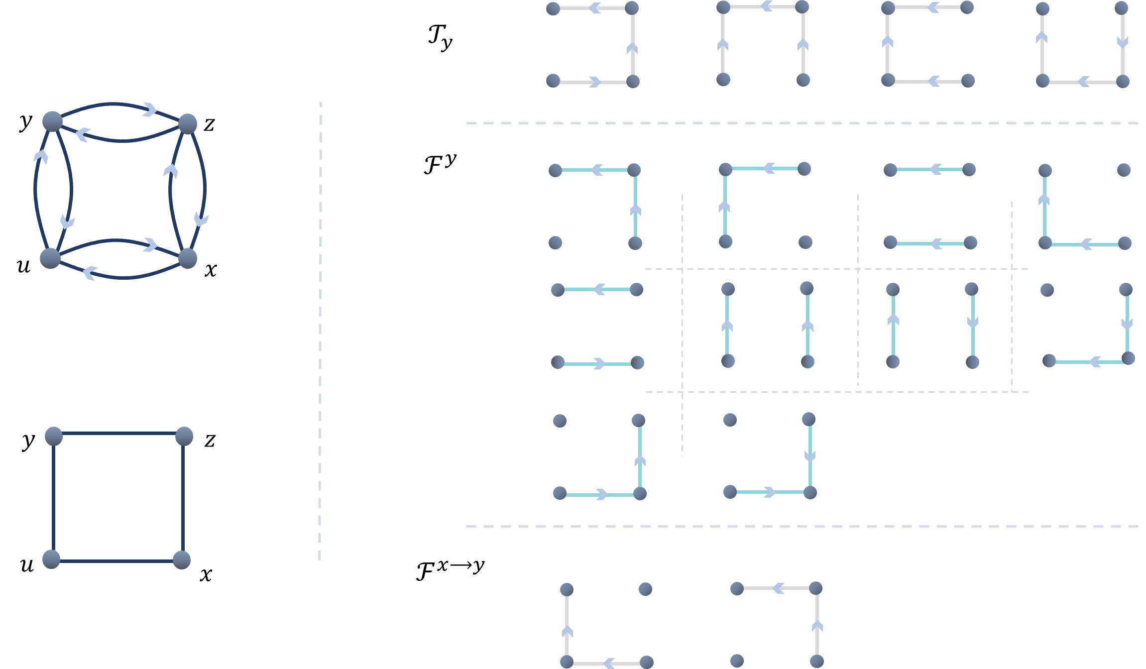
Let xysuperscript𝑥𝑦\mathcal{F}^{x\to y} denote the set of all rooted spanning forests with two trees, where x𝑥x and y𝑦y are in the same tree rooted at y𝑦y. The second tree is rooted as well, and we include all possible orientations. The two-trees, elements of xysuperscript𝑥𝑦\mathcal{F}^{x\to y}, are denoted by Fxysuperscript𝐹𝑥𝑦F^{x\to y}. The weight of the set

w(xy):=w(xy)=Fxyxyw(Fxy),w(Fxy)=(u,u)Fxyk(u,u)formulae-sequenceassign𝑤𝑥𝑦𝑤superscript𝑥𝑦subscriptsuperscript𝐹𝑥𝑦superscript𝑥𝑦𝑤superscript𝐹𝑥𝑦𝑤superscript𝐹𝑥𝑦subscriptproduct𝑢superscript𝑢superscript𝐹𝑥𝑦𝑘𝑢superscript𝑢w(x\to y):=w(\mathcal{F}^{x\to y})=\sum_{F^{x\to y}\in\mathcal{F}^{x\to y}}w(F^{x\to y}),\quad w(F^{x\to y})=\prod_{(u,u^{\prime})\in F^{x\to y}}k(u,u^{\prime}) (IV.2)

We write xx=xsuperscript𝑥𝑥superscript𝑥\mathcal{F}^{x\to x}=\mathcal{F}^{x}; see Fig. 1. Moreover, let x,ysuperscript𝑥𝑦\mathcal{F}^{x,\,y} be the set of all (spanning) forests consisting of two trees such that x𝑥x and y𝑦y are located in different trees and y𝑦y is a root; see Fig. 1 where x,y=yxysuperscript𝑥𝑦superscript𝑦superscript𝑥𝑦\mathcal{F}^{x,\,y}=\mathcal{F}^{y}\setminus\mathcal{F}^{x\to y}.

Refer to caption
Figure 1: A digraph with four vertices (top left) and its simple visualization (down left). Right: from the top onward, the elements of the sets 𝒯ysubscript𝒯𝑦\mathcal{T}_{y}, ysuperscript𝑦\mathcal{F}^{y} and xysuperscript𝑥𝑦\mathcal{F}^{x\to y} are shown.

Recall the Poisson equation (III.2) for the quasipotential V𝑉V, where f𝑓f is a centered function on K𝐾K.

Theorem IV.2.

The solution to (III.2) for Vs=0superscriptdelimited-⟨⟩𝑉𝑠0\langle V\rangle^{s}=0 is

V(x)=yw(xy)Wf(y)𝑉𝑥subscript𝑦𝑤𝑥𝑦𝑊𝑓𝑦V(x)=\sum_{y}\frac{w(x\to y)}{W}\,f(y) (IV.3)

We proceed with the proof by direct verification. An alternative proof, starting from a more general setup and using the Matrix Forest Theorem, is presented in Appendix B.

Proof of Theorem IV.2.
LV(x)𝐿𝑉𝑥\displaystyle LV\,(x) =yk(x,y)[V(y)V(x)]absentsubscript𝑦𝑘𝑥𝑦delimited-[]𝑉𝑦𝑉𝑥\displaystyle=\sum_{y}k(x,y)\,[V(y)-V(x)]
=1Wyk(x,y)z[w(yz)w(xz)]f(z)absent1𝑊subscript𝑦𝑘𝑥𝑦subscript𝑧delimited-[]𝑤𝑦𝑧𝑤𝑥𝑧𝑓𝑧\displaystyle=\frac{1}{W}\,\sum_{y}k(x,y)\,\sum_{z}[w(y\to z)-w(x\to z)]\,f(z)

where w(yz)=w(yz)𝑤𝑦𝑧𝑤superscript𝑦𝑧w(y\to z)=w(\mathcal{F}^{y\to z}) and w(xz)=w(xz)𝑤𝑥𝑧𝑤superscript𝑥𝑧w(x\to z)=w(\mathcal{F}^{x\to z}) as in (IV.2). The intersection of yzsuperscript𝑦𝑧\mathcal{F}^{y\to z} and xzsuperscript𝑥𝑧\mathcal{F}^{x\to z} is the set of all forests where x𝑥x and y𝑦y are located in the same tree. Here, to emphasize the positions x𝑥x and y𝑦y, we use the notation x,yzsuperscript𝑥𝑦𝑧\mathcal{F}^{x,y\to z} to denote the set of all forests where y𝑦y is located in the tree rooted in z𝑧z, and x𝑥x is in the other tree. Then,

LV(x)𝐿𝑉𝑥\displaystyle LV\,(x) =1Wuyk(x,y)[w(x,yz)w(y,xz)]f(z)absent1𝑊subscript𝑢subscript𝑦𝑘𝑥𝑦delimited-[]𝑤superscript𝑥𝑦𝑧𝑤superscript𝑦𝑥𝑧𝑓𝑧\displaystyle=\frac{1}{W}\,\sum_{u}\sum_{y}k(x,y)\,[w(\mathcal{F}^{x,y\to z})-w(\mathcal{F}^{y,x\to z})]\,f(z) (IV.4)

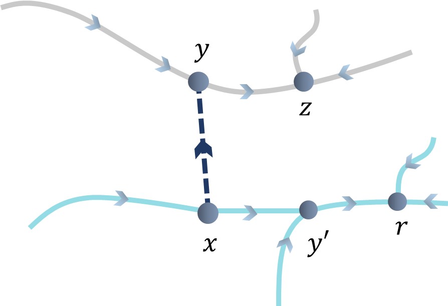
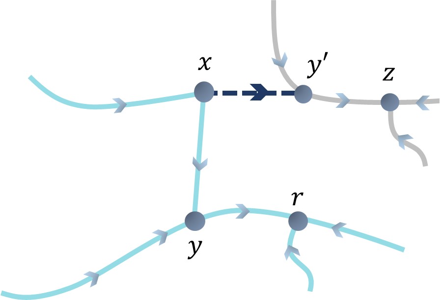
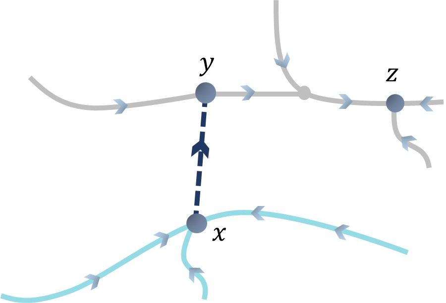
Fix zx𝑧𝑥z\not=x, take a forest Fx,yzx,yzsuperscript𝐹𝑥𝑦𝑧superscript𝑥𝑦𝑧F^{x,y\to z}\in\mathcal{F}^{x,y\to z} and add the edge (x,y)𝑥𝑦(x,y) to that forest: one tree is rooted in z𝑧z, and corresponding to the root of the second tree there are two cases. Consider the case that x𝑥x is not the root, then there exists an edge (x,y)𝑥superscript𝑦(x,y^{\prime}) on the tree. Remove the edge (x,y)𝑥superscript𝑦(x,y^{\prime}) from the graph (x,y)Fx,yz𝑥𝑦superscript𝐹𝑥𝑦𝑧(x,y)\cup F^{x,y\to z}, a new forest is made. The new forest is in the set Fy,xzsuperscript𝐹superscript𝑦𝑥𝑧F^{y^{\prime},x\to z}; see Fig. 2.

Refer to caption
(a) (x,y)Fx,yz𝑥𝑦superscript𝐹𝑥𝑦𝑧(x,y)\cup F^{x,y\to z}
Refer to caption
(b) (x,y)Fy,xz𝑥superscript𝑦superscript𝐹superscript𝑦𝑥𝑧(x,y^{\prime})\cup F^{y^{\prime},x\to z}
Figure 2: Adding (x,y)𝑥𝑦(x,y) to Fx,yzsuperscript𝐹𝑥𝑦𝑧F^{x,y\to z} and the edge (x,y)𝑥superscript𝑦(x,y^{\prime}) to Fy,xzsuperscript𝐹superscript𝑦𝑥𝑧F^{y^{\prime},x\to z}, make the same graphs.

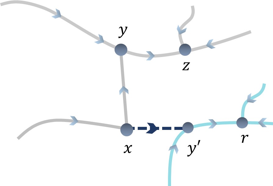
The same scenario is true for the set y,xzsuperscript𝑦𝑥𝑧\mathcal{F}^{y,x\to z}, see Fig. 3.

Refer to caption
(a) (x,y)Fy,xz𝑥𝑦superscript𝐹𝑦𝑥𝑧(x,y)\cup F^{y,x\to z}
Refer to caption
(b) (x,y)Fx,yz𝑥superscript𝑦superscript𝐹𝑥superscript𝑦𝑧(x,y^{\prime})\cup F^{x,y^{\prime}\to z}
Figure 3: Adding (x,y)𝑥𝑦(x,y) to Fy,xzsuperscript𝐹𝑦𝑥𝑧F^{y,x\to z} and the edge (x,y)𝑥superscript𝑦(x,y^{\prime}) to Fx,yzusuperscript𝐹𝑥superscript𝑦𝑧𝑢F^{x,y^{\prime}\to zu}, make the same graphs.

Hence, when x𝑥x is not the root, (IV.4) equals zero.
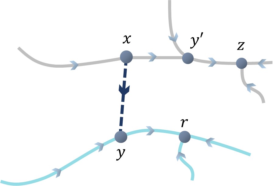
Consider a forest from x,yzsuperscript𝑥𝑦𝑧\mathcal{F}^{x,y\to z}. If x𝑥x is the root of its tree, then adding the edge (x,y)𝑥𝑦(x,y) connects two trees and the new graph is a spanning tree rooted in z𝑧z; see Fig. 4.

Refer to caption
Figure 4: Adding (x,y)𝑥𝑦(x,y) to the forest Fx,yzsuperscript𝐹𝑥𝑦𝑧F^{x,y\to z} where x𝑥x is the root makes a spanning tree rooted in z𝑧z.

Put z=x𝑧𝑥z=x, the set of x,yxsuperscript𝑥𝑦𝑥\mathcal{F}^{x,y\to x} is empty. Take a forest from the set y,xxsuperscript𝑦𝑥𝑥\mathcal{F}^{y,x\to x}. Adding the edge (x,y)𝑥𝑦(x,y) to the forest Fy,xxsuperscript𝐹𝑦𝑥𝑥F^{y,x\to x} again is a new spanning tree rooted on a vertex rx𝑟𝑥r\not=x.
Hence, finally,

LV(x)𝐿𝑉𝑥\displaystyle LV\,(x) =1W[zxw(z)f(z)rxw(r)f(x)]absent1𝑊delimited-[]subscript𝑧𝑥𝑤𝑧𝑓𝑧subscript𝑟𝑥𝑤𝑟𝑓𝑥\displaystyle=\frac{1}{W}[\sum_{z\not=x}w(z)f(z)-\sum_{r\not=x}w(r)f(x)]
=1Wzx[w(z)f(z)w(z)f(x)]absent1𝑊subscript𝑧𝑥delimited-[]𝑤𝑧𝑓𝑧𝑤𝑧𝑓𝑥\displaystyle=\frac{1}{W}\sum_{z\not=x}[w(z)f(z)-w(z)f(x)]
=1Wzx[w(z)f(z)+w(x)f(x)w(x)f(x)w(z)f(x)]absent1𝑊subscript𝑧𝑥delimited-[]𝑤𝑧𝑓𝑧𝑤𝑥𝑓𝑥𝑤𝑥𝑓𝑥𝑤𝑧𝑓𝑥\displaystyle=\frac{1}{W}\sum_{z\not=x}[w(z)f(z)+w(x)f(x)-w(x)f(x)-w(z)f(x)]
=1Wzw(z)f(z)f(x)Wzw(z)=ff(x)absent1𝑊subscript𝑧𝑤𝑧𝑓𝑧𝑓𝑥𝑊subscript𝑧𝑤𝑧delimited-⟨⟩𝑓𝑓𝑥\displaystyle=\frac{1}{W}\sum_{z}w(z)f(z)-\frac{f(x)}{W}\sum_{z}w(z)=\langle f\rangle-f(x)
=f(x)absent𝑓𝑥\displaystyle=-f(x)

where we used the Kirchhoff formula (IV.1) and the fact that f𝑓f is centered. ∎

Next, recall the Poisson equation (III.14) for the mean first-passage times. There as well, we get a graphical representation. The set x,ysuperscript𝑥𝑦\mathcal{F}^{x,y} contains all two-trees with the restrictions:

  • vertices x𝑥x and y𝑦y are in separate trees;

  • the tree that contains y𝑦y is rooted in y𝑦y, while the second tree is rooted anywhere (containing x𝑥x);

  • the weight w(x,y)=w(x,y)𝑤𝑥𝑦𝑤superscript𝑥𝑦w(x,y)=w(\mathcal{F}^{x,y}) of the set of such two-trees Fx,ysuperscript𝐹𝑥𝑦F^{x,y} is

    w(x,y)=Fx,yx,y(u,u)Fx,yk(u,u)𝑤𝑥𝑦subscriptsuperscript𝐹𝑥𝑦superscript𝑥𝑦subscriptproduct𝑢superscript𝑢superscript𝐹𝑥𝑦𝑘𝑢superscript𝑢w(x,y)=\sum_{F^{x,y}\in{\mathcal{F}}^{x,y}}\prod_{(u,u^{\prime})\in F^{x,y}}k(u,u^{\prime})
Theorem IV.3.

The mean first-passage time, solution to (III.14), is

τ(x,z)=w(x,z)w(z)xz;τ(x,x)=0formulae-sequence𝜏𝑥𝑧𝑤𝑥𝑧𝑤𝑧formulae-sequence𝑥𝑧𝜏𝑥𝑥0\tau(x,z)=\frac{w(x,z)}{w(z)}\quad x\neq z;\qquad\tau(x,x)=0 (IV.5)

where w(z)𝑤𝑧w(z) appeared in (IV.1).

We again give the proof of Theorem IV.3 by verification.

Proof of Theorem IV.3.

We need to show

yk(x,y)[w(y,z)w(z)w(x,z)w(z)]=1subscript𝑦𝑘𝑥𝑦delimited-[]𝑤𝑦𝑧𝑤𝑧𝑤𝑥𝑧𝑤𝑧1\sum_{y}k(x,y)[\frac{w(y,z)}{w(z)}-\frac{w(x,z)}{w(z)}]=-1

or

yk(x,y)[w(x,z)w(y,z)]=w(z).subscript𝑦𝑘𝑥𝑦delimited-[]𝑤𝑥𝑧𝑤𝑦𝑧𝑤𝑧\sum_{y}k(x,y)[w(x,z)-w(y,z)]=w(z). (IV.6)

where w(x,z)=w(x,z)𝑤𝑥𝑧𝑤superscript𝑥𝑧w(x,z)=w(\mathcal{F}^{x,\,z}) and w(y,z)=w(y,z)𝑤𝑦𝑧𝑤superscript𝑦𝑧w(y,z)=w(\mathcal{F}^{y,\,z}),

w(x,z)w(y,z)𝑤𝑥𝑧𝑤𝑦𝑧\displaystyle w(x,z)-w(y,z) =Fx,zx,zw(Fx,z)Fy,zy,zw(Fy,z)absentsubscriptsuperscript𝐹𝑥𝑧superscript𝑥𝑧𝑤superscript𝐹𝑥𝑧subscriptsuperscript𝐹𝑦𝑧superscript𝑦𝑧𝑤superscript𝐹𝑦𝑧\displaystyle=\sum_{F^{x,\,z}\in\mathcal{F}^{x,\,z}}w(F^{x,\,z})-\sum_{F^{y,\,z}\in\mathcal{F}^{y,\,z}}w(F^{y,\,z})

The intersection of the sets x,zsuperscript𝑥𝑧\mathcal{F}^{x,\,z} and y,zsuperscript𝑦𝑧\mathcal{F}^{y,\,z} is a set of forests where x𝑥x and y𝑦y are located in the same tree. We only consider the sets of forests where x𝑥x and y𝑦y are in different trees,

w(x,z)w(y,z)𝑤𝑥𝑧𝑤𝑦𝑧\displaystyle w(x,z)-w(y,z) =w(x,yz)w(y,xz)absent𝑤superscript𝑥𝑦𝑧𝑤superscript𝑦𝑥𝑧\displaystyle=w(\mathcal{F}^{x,y\to z})-w(\mathcal{F}^{y,x\to z})

x,yzsuperscript𝑥𝑦𝑧\mathcal{F}^{x,y\to z} denotes the set of all forests, where x𝑥x and z𝑧z are in the different trees and y𝑦y is in the same tree with z𝑧z.
Take a forest Fx,yzsuperscript𝐹𝑥𝑦𝑧F^{x,y\to z} from the set x,yzsuperscript𝑥𝑦𝑧\mathcal{F}^{x,y\to z}. We consider two cases based on whether x𝑥x is a root or not. If x𝑥x is not the root in forest Fx,yzsuperscript𝐹𝑥𝑦𝑧F^{x,y\to z}, then x𝑥x has a neighbor such as ysuperscript𝑦y^{\prime}. Add the edge (x,y)𝑥𝑦(x,y) where y𝑦y is located in the same tree as z𝑧z: a directed graphical object is created; see Fig. 2 (a). The new graphical object is created also by adding edge (x,y)𝑥superscript𝑦(x,y^{\prime}) to a forest from the set y,xzsuperscriptsuperscript𝑦𝑥𝑧\mathcal{F}^{y^{\prime},x\to z}, where x𝑥x and z𝑧z are located in the same tree in the forest and ysuperscript𝑦y^{\prime} is in another tree; see Fig. 2 (b). The same graphical objects have equal weights.
If x𝑥x is a root, adding the edge (x,y)𝑥𝑦(x,y) connects two trees and creates a new spanning tree rooted at z𝑧z; see Fig. 4. Consider a spanning tree rooted at vertex z𝑧z, where each of the other vertices has an outgoing edge. Remove the edge that goes out from x𝑥x: a forest in the set x,zsuperscript𝑥𝑧\mathcal{F}^{x,\,z} is created. That ends the proof. ∎

Corollary IV.4.

Independently of x𝑥x,

yρs(y)τ(x,y)=W2Wsubscript𝑦superscript𝜌𝑠𝑦𝜏𝑥𝑦subscript𝑊2𝑊\sum_{y}\rho^{s}(y)\tau(x,y)=\frac{W_{2}}{W} (IV.7)

where W2subscript𝑊2W_{2} is the total weight of all spanning two-tree forests with both trees subsequently oriented toward all its states.

Proof of (IV.7).
yρs(y)τ(x,y)subscript𝑦superscript𝜌𝑠𝑦𝜏𝑥𝑦\displaystyle\sum_{y}\rho^{s}(y)\tau(x,y) =yw(x,y)w(y)w(y)W=1Wyw(x,y)absentsubscript𝑦𝑤𝑥𝑦𝑤𝑦𝑤𝑦𝑊1𝑊subscript𝑦𝑤𝑥𝑦\displaystyle=\sum_{y}\frac{w(x,y)}{w(y)}\,\frac{w(y)}{W}=\frac{1}{W}\sum_{y}w(x,y)

and

W2=yw(x,y)subscript𝑊2subscript𝑦𝑤𝑥𝑦W_{2}=\sum_{y}w(x,y)

for every y𝑦y, there is a forest Fx,yx,ysuperscript𝐹𝑥𝑦superscript𝑥𝑦F^{x,y}\in\mathcal{F}^{x,y} where x𝑥x is the root and for all yx𝑦𝑥y\not=x also y𝑦y is the root. So then W2subscript𝑊2W_{2} is the weight of the set of all forests with two rooted trees and it is independent of x𝑥x. ∎

V Bounds

One important issue for possible applications of the Poisson equation is to get bounds on its solution. One could imagine in fact a parameterized family of Poisson equations and the issue becomes to get bounds that are uniform in that parameterization. The present section adds such bounds, as a consequence of the previous sections.

V.1 Via mean first-passage times

Consider the centered solution V𝑉V of the Poisson equation (III.2), with f:=maxzK|f(z)fs|assignnorm𝑓subscript𝑧𝐾𝑓𝑧superscriptdelimited-⟨⟩𝑓𝑠||f||:=\max_{z\in K}|f(z)-\langle f\rangle^{s}|. Fix any two states x,yK𝑥𝑦𝐾x,y\in K, and put

v~(x,y):=0TK{y}dt[f(Xt)fs]|X0=xassign~𝑣𝑥𝑦inner-productsuperscriptsubscript0subscript𝑇𝐾𝑦d𝑡delimited-[]𝑓subscript𝑋𝑡superscriptdelimited-⟨⟩𝑓𝑠subscript𝑋0𝑥\tilde{v}(x,y):=\left\langle\int_{0}^{T_{K\setminus\{y\}}}\textrm{d}t\,[f(X_{t})-\langle f\rangle^{s}]\,|\,X_{0}=x\right\rangle (V.1)

as the expected first-passage accumulation for the centered observable ffs𝑓superscriptdelimited-⟨⟩𝑓𝑠f-\langle f\rangle^{s}.

Theorem V.1.

We have

V(x)V(y)=v~(x,y)𝑉𝑥𝑉𝑦~𝑣𝑥𝑦V(x)-V(y)=\tilde{v}(x,y) (V.2)

and the bound

|V(x)V(y)|fmin{τ(x,y),τ(y,x)}𝑉𝑥𝑉𝑦norm𝑓𝜏𝑥𝑦𝜏𝑦𝑥|V(x)-V(y)|\leq||f||\min\{\tau(x,y),\tau(y,x)\} (V.3)
Proof of Theorem V.1.

To prove (V.2), we note that the centered solution V(x)𝑉𝑥V(x) to (III.2) can be written by fixing state y𝑦y, and decomposing as

V(x)=limt0TK{y}f(X(t))dt+TK{y}tf(X(t))dtfstx=ϕK{y}(x)fsTK{y}x+limt0t[f(X(t))fs]dty=VK{y}(x)fs𝔖K{y}(x)+V(y)\begin{split}V(x)&=\lim_{t\to\infty}\Bigl{\langle}\int_{0}^{T_{K\setminus\{y\}}}f(X(t^{\prime}))\,\textrm{d}t^{\prime}+\int_{T_{K\setminus\{y\}}}^{t}f(X(t^{\prime}))\,\textrm{d}t^{\prime}-\langle f\rangle^{s}t\Bigr{\rangle}_{x}\\ &=\Bigl{\langle}\phi_{K\setminus\{y\}}(x)-\langle f\rangle^{s}\,\langle T_{K\setminus\{y\}}\rangle_{x}+\lim_{t\to\infty}\Bigl{\langle}\int_{0}^{t}[f(X(t^{\prime}))-\langle f\rangle^{s}]\,\textrm{d}t^{\prime}\Bigr{\rangle}_{y}\\ &=V_{K\setminus\{y\}}(x)-\langle f\rangle^{s}{\mathfrak{S}}_{K\setminus\{y\}}(x)+V(y)\end{split} (V.4)

where in the limit of the second integral we have used the exponential tightness of TK{y}subscript𝑇𝐾𝑦T_{K\setminus\{y\}}. As before, 𝔖K{y}(x)=τ(x,y)subscript𝔖𝐾𝑦𝑥𝜏𝑥𝑦{\mathfrak{S}}_{K\setminus\{y\}}(x)=\tau(x,y) is the mean first-passage time to reach y𝑦y from x𝑥x, and VK{y}(x)=:v(x,y)V_{K\setminus\{y\}}(x)=:v(x,y) is the expected accumulation for f𝑓f up to the first passage a y𝑦y, as in Section III.2. Therefore, we have the relation

V(x)V(y)=v(x,y)fsτ(x,y)=v~(x,y)𝑉𝑥𝑉𝑦𝑣𝑥𝑦superscriptdelimited-⟨⟩𝑓𝑠𝜏𝑥𝑦~𝑣𝑥𝑦\begin{split}V(x)-V(y)&=v(x,y)-\langle f\rangle^{s}\,\tau(x,y)\\ &=\tilde{v}(x,y)\end{split} (V.5)

with v~(x,y)~𝑣𝑥𝑦\tilde{v}(x,y) defined in (V.1).
Finally, from the very definition of v~(x,y)~𝑣𝑥𝑦\tilde{v}(x,y)

|v~(x,y)|fτ(x,y)~𝑣𝑥𝑦norm𝑓𝜏𝑥𝑦|\tilde{v}(x,y)|\leq||f||\,\tau(x,y)

Moreover, from (V.2), v~(x,y)=v~(y,x)~𝑣𝑥𝑦~𝑣𝑦𝑥\tilde{v}(x,y)=-\tilde{v}(y,x) is antisymmetric, which yields the bound (V.3). ∎

Note that since Vs=0superscriptdelimited-⟨⟩𝑉𝑠0\langle V\rangle^{s}=0, there are always states x0,x1Ksubscript𝑥0subscript𝑥1𝐾x_{0},x_{1}\in K with V(x0)0V(x1)𝑉subscript𝑥00𝑉subscript𝑥1V(x_{0})\leq 0\leq V(x_{1}). Therefore, for every xK𝑥𝐾x\in K,

V(x)V(x)V(x0)x0x|V(xi)V(xi+1)|𝑉𝑥𝑉𝑥𝑉subscript𝑥0subscriptsubscript𝑥0𝑥𝑉subscript𝑥𝑖𝑉subscript𝑥𝑖1V(x)\leq V(x)-V(x_{0})\leq\sum_{x_{0}\rightarrow x}|V(x_{i})-V(x_{i+1})|

where the sum is over an arbitrary path in K𝐾K connecting x0subscript𝑥0x_{0} and x𝑥x. Similarly,

V(x)V(x)V(x1)x1x|V(xi)V(xi+1)|𝑉𝑥𝑉𝑥𝑉subscript𝑥1subscriptsubscript𝑥1𝑥𝑉subscript𝑥𝑖𝑉subscript𝑥𝑖1V(x)\geq V(x)-V(x_{1})\geq-\sum_{x_{1}\rightarrow x}|V(x_{i})-V(x_{i+1})|

As a consequence, bounds on the solution V𝑉V follow from bounds on the differences, as provided in (V.3).

The bound (V.3) is not always optimal. It still can be improved as follows.

Theorem V.2.

Suppose there exists a set 𝒟𝒟\mathcal{D} so that f(x)=LE(x)+h(x)𝑓𝑥𝐿𝐸𝑥𝑥f(x)=LE(x)+h(x) where h=hEsubscript𝐸h=h_{E} depends on E𝐸E and h(x)=0𝑥0h(x)=0 for x𝒟𝑥𝒟x\notin\mathcal{D}. Then, the solution of the Poisson equation (III.2) V𝑉V satisfies

|V(x)V(y)||E(x)E(y)|+hEz𝒟ρs(z)|τ(x,z)τ(y,z)|𝑉𝑥𝑉𝑦𝐸𝑥𝐸𝑦normsubscript𝐸subscript𝑧𝒟superscript𝜌𝑠𝑧𝜏𝑥𝑧𝜏𝑦𝑧|V(x)-V(y)|\leq|E(x)-E(y)|+||h_{E}||\sum_{z\in{\mathcal{D}}}\rho^{s}(z)|\tau(x,z)-\tau(y,z)| (V.6)

That bound requires to control the accessibility of the set 𝒟𝒟\mathcal{D} only. In fact, since there is a freedom in choosing (E,h)𝐸(E,h), that can be used to optimize the bound (V.6). We observe that in the case where fLE𝑓𝐿𝐸f\equiv LE, the bound is optimal because then V=E+constant𝑉𝐸constantV=E+\text{constant}.

Proof of Theorem V.2.

The Poisson equation now becomes

L(V+E)+h=0, with h=0 on K𝒟formulae-sequence𝐿𝑉𝐸0 with 0 on 𝐾𝒟L(V+E)+h=0,\quad\text{ with }h=0\text{ on }K\setminus\mathcal{D}

Applying (III.15), we get

V(x)+E(x)=z𝒟ρs(z)hE(z)τ(x,z)+constant𝑉𝑥𝐸𝑥subscript𝑧𝒟superscript𝜌𝑠𝑧subscript𝐸𝑧𝜏𝑥𝑧constantV(x)+E(x)=-\sum_{z\in\mathcal{D}}\rho^{s}(z)\,h_{E}(z)\,\tau(x,z)+\text{constant} (V.7)

and the bound (V.6) follows directly. ∎

V.2 Via graphical representation

We recall the setup where a digraph with n𝑛n vertices is obtained from a Markov jump process with transition rates k(u,u)𝑘𝑢superscript𝑢k(u,u^{\prime}). We define

f:=maxy|f(y)|,k:=max(u,u)k(u,u)formulae-sequenceassignnorm𝑓subscript𝑦𝑓𝑦assignnorm𝑘subscript𝑢superscript𝑢𝑘𝑢superscript𝑢||f||:=\max_{y}|f(y)|,\quad||k||:=\max_{(u,u^{\prime})}k(u,u^{\prime}) (V.8)
Theorem V.3.

For all x𝑥x,

|V(x)|nkn2Wf𝑉𝑥𝑛superscriptnorm𝑘𝑛2𝑊norm𝑓|V(x)|\leq\frac{n\,||k||^{n-2}}{W}\,||f|| (V.9)
Proof of Theorem V.3.

We apply (IV.3) of Theorem IV.2. The product over the weights over edges is obviously bounded, and the weight of any forest in the graph is bounded as well. In other words, for any x𝑥x and y𝑦y in the graph, w(xy)𝑤𝑥𝑦w(x\to y) is bounded.
Using (V.8),

w(xy)f(y)fkn2𝑤𝑥𝑦𝑓𝑦norm𝑓superscriptnorm𝑘𝑛2w(x\to y)f(y)\leq\,||f||\,||k||^{n-2}

and the result follows from (IV.3). ∎

As an application of (V.9), we can suppose that the rates k(x,y)=kλ(x,y)𝑘𝑥𝑦subscript𝑘𝜆𝑥𝑦k(x,y)=k_{\lambda}(x,y) depend on a real-valued parameter λ𝜆\lambda. For simplicity, we consider the limit λ𝜆\lambda\rightarrow\infty (taking for λ𝜆\lambda the inverse temperature is a relevant example from statistical mechanics). Observe that there is a general lower bound on W𝑊W, i.e., WmaxT,xw(Tx)𝑊subscript𝑇𝑥𝑤subscript𝑇𝑥W\geq\max_{T,x}w(T_{x}), the largest weight of all spanning trees. Hence, if there exists a spanning tree with w(Tx)>0𝑤subscript𝑇𝑥0w(T_{x})>0 uniformly in λ𝜆\lambda, then W=Wλ>0𝑊subscript𝑊𝜆0W=W_{\lambda}>0 is uniformly bounded, and (V.9) gives a uniform bound on V𝑉V.
The bound (V.9) can for instance be used in an argument extending the Third Law of Thermodynamics to nonequilibrium systems; see jchemphys where the source function f𝑓f is the expected heat flux. The quasipotential V𝑉V in (III.4) is then the time-integral of the difference between the instantaneous heat flux and the stationary heat flux.

VI Conclusions

The Poisson equation is ubiquitous in mathematical physics. We have considered a setup where the linear operator is the backward generator of a Markov jump process and the functions are defined on the possible (finite number of) states. We have related the solution of that discrete Poisson equation to the formalism of mean first-passage times, and we have given graphical representations that allow precise estimates—both for the accumulations before first hitting a particular state when starting from another one, and for the quasipotentials measuring the accumulated excess during relaxation to stationarity. The results do not assume reversibility, and are ready to be used in extensions of potential theory when applied to problems in steady-nonequilibrium statistical mechanics. Obvious targets are reaction rate theory for driven or active systems, and metastability around nonequilibrium steady conditions.

Appendix A On proving the Kirchhoff formula

The Kirchhoff formula can be seen as a consequence of the Matrix Tree Theorem, shubertkir ; tutte1948dissection ; kirphi . However, there also exists a more probabilistic approach. The ideas is illustrated by the algorithm in Fig. 5, where a tree Txsubscriptsuperscript𝑇𝑥T^{\prime}_{x} is constructed by removing the edge (x,y)𝑥superscript𝑦(x,y^{\prime}) from the tree Tysubscript𝑇𝑦T_{y}, and then adding the edge (y,x)𝑦𝑥(y,x). That algorithm is used in kirana to construct a reversible Markov chain Ynsubscript𝑌𝑛Y_{n} on an ensemble of trees, where the states are the rooted spanning trees and jumps are possible if and only if the corresponding trees are connected by the above-mentioned algorithm. Let Qab=q(a,b)subscript𝑄𝑎𝑏𝑞𝑎𝑏Q_{ab}=q(a,b) be the stochastic matrix of Ynsubscript𝑌𝑛Y_{n}, and put π𝜋\pi the stationary distribution of Q𝑄Q. For example, we can assign states a𝑎a and b𝑏b, respectively, to the trees Tysubscript𝑇𝑦T_{y} and Txsubscriptsuperscript𝑇𝑥T^{\prime}_{x} in Fig. 5, and take transition rates q(a,b)𝑞𝑎𝑏q(a,b). It is shown that putting q(a,b)=k(y,x)𝑞𝑎𝑏𝑘𝑦𝑥q(a,b)=k(y,x), q(b,a)=k(x,y)𝑞𝑏𝑎𝑘𝑥superscript𝑦q(b,a)=k(x,y^{\prime}) produces detailed balance πaq(a,b)=πbq(b,a)subscript𝜋𝑎𝑞𝑎𝑏subscript𝜋𝑏𝑞𝑏𝑎\pi_{a}q(a,b)=\pi_{b}q(b,a). We add a sketch of the proof.

It suffices to show that the Kirchhoff formula (IV.1) satisfies the stationary Master equation,

yw(y)k(y,x)w(x)k(x,y)=0subscript𝑦𝑤𝑦𝑘𝑦𝑥𝑤𝑥𝑘𝑥𝑦0\sum_{y}w(y)k(y,x)-w(x)k(x,y)=0

Take a spanning tree rooted in y𝑦y, Ty𝒯ysubscript𝑇𝑦subscript𝒯𝑦T_{y}\in\mathcal{T}_{y}. Let x𝑥x be a vertex located on the tree Tysubscript𝑇𝑦T_{y}. In this case, x𝑥x is not the root and there exists a vertex ysuperscript𝑦y^{\prime} (which may be equal to y𝑦y) and an edge (x,y)𝑥superscript𝑦(x,y^{\prime}) which goes out from x𝑥x and connects x𝑥x to the tree. By removing the edge (x,y)𝑥superscript𝑦(x,y^{\prime}) from the tree Tysubscript𝑇𝑦T_{y} and adding the edge (y,x)𝑦𝑥(y,x), a new spanning tree rooted in x𝑥x is created; see Fig. 5.

Refer to caption
Figure 5: Removing the edge (x,y)𝑥superscript𝑦(x,y^{\prime}) from the spanning tree Tysubscript𝑇𝑦T_{y} and adding the edge (y,x)𝑦𝑥(y,x) creates a spanning tree rooted in x𝑥x.

It turns out that w(Ty)k(x,y)=w(Tx)k(y,x)𝑤subscript𝑇𝑦𝑘𝑥superscript𝑦𝑤subscriptsuperscript𝑇𝑥𝑘𝑦𝑥\dfrac{w(T_{y})}{k(x,y^{\prime})}=\dfrac{w(T^{\prime}_{x})}{k(y,x)}. With the same scenario, from every spanning tree rooted in y𝑦y we can make a new spanning tree rooted in x𝑥x. That algorithm makes a spanning tree rooted in y𝑦y from a spanning tree rooted in x𝑥x. Therefore,

yw(y)k(y,x)=yTy𝒯yw(Ty)k(y,x)=yTx𝒯xw(Tx)k(x,y)=yw(x)k(x,y)subscript𝑦𝑤𝑦𝑘𝑦𝑥subscript𝑦subscriptsubscript𝑇𝑦subscript𝒯𝑦𝑤subscript𝑇𝑦𝑘𝑦𝑥subscriptsuperscript𝑦subscriptsubscriptsuperscript𝑇𝑥subscript𝒯𝑥𝑤subscriptsuperscript𝑇𝑥𝑘𝑥superscript𝑦subscriptsuperscript𝑦𝑤𝑥𝑘𝑥superscript𝑦\displaystyle\sum_{y}w(y)k(y,x)=\sum_{y}\sum_{T_{y}\in\mathcal{T}_{y}}w(T_{y})k(y,x)=\sum_{y^{\prime}}\sum_{T^{\prime}_{x}\in\mathcal{T}_{x}}w(T^{\prime}_{x})k(x,y^{\prime})=\sum_{y^{\prime}}w(x)k(x,y^{\prime})

which ends the proof.

Appendix B Matrix Forest Theorem

The present Appendix gives the broader mathematical context of the graphical representations.

B.1 Laplacian matrix and the backward generator

Consider a self edge-free directed graph 𝒢(𝒱(𝒢),(𝒢))𝒢𝒱𝒢𝒢\mathcal{G}(\mathcal{V}(\mathcal{G}),\mathcal{E}(\mathcal{G})), with n𝑛n vertices and 𝔪𝔪{\mathfrak{m}} edges. The adjacency matrix A(𝒢)𝐴𝒢A(\mathcal{G}) is a n×n𝑛𝑛n\times n matrix with elements A(𝒢)x,y=wx,y𝐴subscript𝒢𝑥𝑦subscript𝑤𝑥𝑦A(\mathcal{G})_{x,y}=w_{x,y}.
The out-weight of a vertex x𝒱(G)𝑥𝒱𝐺x\in\mathcal{V}(G) is the sum ywx,ysubscript𝑦subscript𝑤𝑥𝑦\sum_{y}w_{x,y}, and we define the n×n𝑛𝑛n\times n diagonal matrix D(G)𝐷𝐺D(G) with Dx,y=0subscript𝐷𝑥𝑦0D_{x,y}=0 if xy𝑥𝑦x\not=y and otherwise Dx,x=ywx,ysubscript𝐷𝑥𝑥subscript𝑦subscript𝑤𝑥𝑦D_{x,x}=\sum_{y}w_{x,y}.
The Laplacian matrix for a directed graph 𝒢𝒢\mathcal{G} is,

(𝒢)=D(𝒢)A(𝒢).𝒢𝐷𝒢𝐴𝒢\mathcal{L}(\mathcal{G})=D(\mathcal{G})-A(\mathcal{G}). (B.1)

Clearly, (𝒢)𝒢\mathcal{L}(\mathcal{G}) is not always symmetric, and the backward generator of the Markov jump process (as we had it in Section II) L=𝐿L=-\mathcal{L} is minus the Laplacian matrix of the underlining graph when putting wx,y=k(x,y)subscript𝑤𝑥𝑦𝑘𝑥𝑦w_{x,y}=k(x,y). Therefore, all properties of the Laplacian of a weighted digraph, as described in section B.1, also hold for the backward generator L𝐿L, as described in Section II.

The Laplacian matrix of a (directed) graph has several important properties that have been extensively studied in the literature chebo2002 ; adi .

B.2 Pseudo-inverses of the Laplacian matrix

The Laplacian is not invertible, and different pseudo/generalized-inverses can be defined, e.g. group inverse, Drazin inverse, Moore–Penrose inverse and resolvent inverse. Depending on the characteristics of the graph, the different inverses of the Laplacian can be equal or not; see also drazin .

As a reminder, for an arbitrary square matrix A𝐴A, its Drazin inverse is denoted by ADsuperscript𝐴𝐷A^{D} and is the unique matrix X𝑋X satisfying the following equations

Aν+1X=XAν,XAX=X,AX=XAformulae-sequencesuperscript𝐴𝜈1𝑋𝑋superscript𝐴𝜈formulae-sequence𝑋𝐴𝑋𝑋𝐴𝑋𝑋𝐴A^{\nu+1}\,X=X\,A^{\nu},\quad X\,A\,X=X,\quad A\,X=X\,A (B.2)

where ν=indA𝜈ind𝐴\nu=\text{ind}\,A (remember indAind𝐴\text{ind}\,A is the smallest non negative integer number b𝑏b such that rank(Ab+1)=rank(Ab)ranksuperscript𝐴𝑏1ranksuperscript𝐴𝑏\text{rank}(A^{b+1})=\text{rank}(A^{b})). If ν=0𝜈0\nu=0, then AD=A1superscript𝐴𝐷superscript𝐴1A^{D}=A^{-1}; if ν1𝜈1\nu\leq 1, then ADsuperscript𝐴𝐷A^{D} is referred to the group inverse and it is denoted by A#superscript𝐴#A^{\#} which is a unique matrix such as X𝑋X satisfying the following equations

AXA=A,XAX=X,AX=XAformulae-sequence𝐴𝑋𝐴𝐴formulae-sequence𝑋𝐴𝑋𝑋𝐴𝑋𝑋𝐴A\,X\,A=A,\quad X\,A\,X=X,\quad A\,X=X\,A (B.3)

As a consequence, when the index of a matrix is one its Drazin inverse and group inverse are the same; see B.2.

We refer to chebo2006max for the Matrix Forest Theorem for a Laplacian matrix. We briefly recall that result.

Consider a weighted digraph 𝒢𝒢\mathcal{G}, where n𝑛n is the number of vertices. I𝐼I is the identity matrix, mxysubscriptsuperscript𝑥𝑦𝑚\mathcal{F}^{x\to y}_{m} is the set of all forests with m𝑚m edges such that x𝑥x and y𝑦y are in the same tree and y𝑦y is always a root, msubscript𝑚\mathcal{F}_{m} is the union of all mxsubscriptsuperscript𝑥𝑚\mathcal{F}^{x}_{m}, and m𝑚m is the number of edges making the forests. For example, if m=n1𝑚𝑛1m=n-1 the forests are made by one spanning tree with n1𝑛1n-1 edges, and when m=n2𝑚𝑛2m=n-2 the forest has two trees. w(mxy)𝑤subscriptsuperscript𝑥𝑦𝑚w(\mathcal{F}^{x\to y}_{m}) is the weight of the set mxysubscriptsuperscript𝑥𝑦𝑚\mathcal{F}^{x\to y}_{m}. γ𝛾\gamma is the dimension of the forest in 𝒢𝒢\mathcal{G}. Forest dimension is the minimum number of rooted trees that a spanning rooted forest can have in a directed graph. Note that when the graph is strongly connected γ=1𝛾1\gamma=1.

Consider a weighted digraph 𝒢𝒢\mathcal{G} with the Laplacian matrix \mathcal{L}. From chebo2006matrixforest ,

Theorem B.1.

For any α>0𝛼0\alpha>0, the matrix (I+α(𝒢))1superscript𝐼𝛼𝒢1(I+\alpha\,\mathcal{L}(\mathcal{G}))^{-1} has the graphical representation

(1I+α)x,y=m=0nγαmw(mxy)m=0nγαmw(m)subscript1𝐼𝛼𝑥𝑦superscriptsubscript𝑚0𝑛𝛾superscript𝛼𝑚𝑤subscriptsuperscript𝑥𝑦𝑚superscriptsubscript𝑚0𝑛𝛾superscript𝛼𝑚𝑤subscript𝑚\displaystyle\bigg{(}\dfrac{1}{I+\alpha\,\mathcal{L}}\bigg{)}_{x,y}=\frac{\sum_{m=0}^{n-\gamma}\alpha^{m}w(\mathcal{F}^{x\to y}_{m})}{\sum_{m=0}^{n-\gamma}\alpha^{m}w(\mathcal{F}_{m})} (B.4)

For the specific case when γ=1𝛾1\gamma=1,

(1I+α)x,y=m=0n2αmw(mxy)m=0n1αmw(m)+αn1w(𝒯y)m=0n1αmw(m)subscript1𝐼𝛼𝑥𝑦superscriptsubscript𝑚0𝑛2superscript𝛼𝑚𝑤subscriptsuperscript𝑥𝑦𝑚superscriptsubscript𝑚0𝑛1superscript𝛼𝑚𝑤subscript𝑚superscript𝛼𝑛1𝑤subscript𝒯𝑦superscriptsubscript𝑚0𝑛1superscript𝛼𝑚𝑤subscript𝑚\displaystyle\bigg{(}\dfrac{1}{I+\alpha\,\mathcal{L}}\bigg{)}_{x,y}=\frac{\sum_{m=0}^{n-2}\alpha^{m}w(\mathcal{F}^{x\to y}_{m})}{\sum_{m=0}^{n-1}\alpha^{m}w(\mathcal{F}_{m})}+\frac{\alpha^{n-1}w(\mathcal{T}_{y})}{\sum_{m=0}^{n-1}\alpha^{m}w(\mathcal{F}_{m})} (B.5)

where we have used n1xy=𝒯ysubscriptsuperscript𝑥𝑦𝑛1subscript𝒯𝑦\mathcal{F}^{x\to y}_{n-1}=\mathcal{T}_{y}, i.e., the forest with n1𝑛1n-1 edges is a spanning tree. w(𝒯y)𝑤subscript𝒯𝑦w(\mathcal{T}_{y}) is the weight of the set 𝒯ysubscript𝒯𝑦\mathcal{T}_{y}, w(𝒯y)=w(y).𝑤subscript𝒯𝑦𝑤𝑦w(\mathcal{T}_{y})=w(y).

From chebo2002 ; chebofpt the graphical representation for the group inverse of #superscript#\mathcal{L}^{\#} is,

Theorem B.2.
x,y#=1w(nγ)(w(nγ1xy)w(nγ1)w(nγxy)w(nγ))subscriptsuperscript#𝑥𝑦1𝑤subscript𝑛𝛾𝑤superscriptsubscript𝑛𝛾1𝑥𝑦𝑤subscript𝑛𝛾1𝑤superscriptsubscript𝑛𝛾𝑥𝑦𝑤subscript𝑛𝛾\mathcal{L}^{\#}_{x,y}=\frac{1}{w(\mathcal{F}_{n-\gamma})}\big{(}w(\mathcal{F}_{n-\gamma-1}^{x\to y})-w(\mathcal{F}_{n-\gamma-1})\frac{w(\mathcal{F}_{n-\gamma}^{x\to y})}{w(\mathcal{F}_{n-\gamma})}\big{)} (B.6)

If γ=1𝛾1\gamma=1

x,y#subscriptsuperscript#𝑥𝑦\displaystyle\mathcal{L}^{\#}_{x,y} =1w(n1)(w(xy)w()w(n1xy)w(n1))absent1𝑤subscript𝑛1𝑤superscript𝑥𝑦𝑤𝑤superscriptsubscript𝑛1𝑥𝑦𝑤subscript𝑛1\displaystyle=\frac{1}{w(\mathcal{F}_{n-1})}\big{(}w(\mathcal{F}^{x\to y})-w(\mathcal{F})\,\frac{w(\mathcal{F}_{n-1}^{x\to y})}{w(\mathcal{F}_{n-1})}\big{)}
=1yw(𝒯y)(w(xy)w()w(𝒯y)yw(𝒯y))absent1subscript𝑦𝑤subscript𝒯𝑦𝑤superscript𝑥𝑦𝑤𝑤subscript𝒯𝑦subscript𝑦𝑤subscript𝒯𝑦\displaystyle=\frac{1}{\sum_{y}w(\mathcal{T}_{y})}\big{(}w(\mathcal{F}^{x\to y})-w(\mathcal{F})\,\frac{w(\mathcal{T}_{y})}{\sum_{y}w(\mathcal{T}_{y})}\big{)} (B.7)
=1W(w(xy)w()ρs(y))absent1𝑊𝑤superscript𝑥𝑦𝑤superscript𝜌𝑠𝑦\displaystyle=\frac{1}{W}\big{(}w(\mathcal{F}^{x\to y})-w(\mathcal{F})\,\rho^{s}(y)\big{)} (B.8)

where we have used that the set of all rooted spanning forests with n1𝑛1n-1 edges is indeed the set of all rooted spanning trees. \mathcal{F} denotes the set of all rooted spanning forests consisting of two trees. In the last line we used the Kirchhoff formula.

The group inverse of the backward generator is denoted by L#superscript𝐿#L^{\#} and from Theorem B.2 the graphical representation is

Lx,y#=w(xy)W+ρ(y)w()Wsubscriptsuperscript𝐿#𝑥𝑦𝑤superscript𝑥𝑦𝑊𝜌𝑦𝑤𝑊\displaystyle L^{\#}_{x,y}=-\frac{w(\mathcal{F}^{x\to y})\,}{W}+\rho(y)\,\,\frac{w(\mathcal{F})}{W} (B.9)

B.3 Another proof of Theorem IV.2

We can solve the equation (III.2)italic-(III.2italic-)\eqref{prop} by utilizing a graphical representation of the pseudoinverse of L𝐿L, which can be obtained through the application of the Matrix Forest Theorem.

Proof.

Let us assume that f𝑓f is centered, meaning yf(y)ρs(y)=0subscript𝑦𝑓𝑦superscript𝜌𝑠𝑦0\sum_{y}f(y)\,\rho^{s}(y)=0. Use the graphical representation (B.4),

V(x)𝑉𝑥\displaystyle V(x) =limαy(αIαL)x,yf(y)absentsubscript𝛼subscript𝑦subscript𝛼𝐼𝛼𝐿𝑥𝑦𝑓𝑦\displaystyle=\lim_{\alpha\to\infty}\sum_{y}\bigg{(}\dfrac{\alpha}{I-\alpha\,L}\bigg{)}_{x,y}\,f(y)
=limαym=0n2αm+1w(mxy)m=0n1αmw(m)+limαyαnw(𝒯y)m=0n1αmw(m)f(y)absentsubscript𝛼subscript𝑦superscriptsubscript𝑚0𝑛2superscript𝛼𝑚1𝑤subscriptsuperscript𝑥𝑦𝑚superscriptsubscript𝑚0𝑛1superscript𝛼𝑚𝑤subscript𝑚subscript𝛼subscript𝑦superscript𝛼𝑛𝑤subscript𝒯𝑦superscriptsubscript𝑚0𝑛1superscript𝛼𝑚𝑤subscript𝑚𝑓𝑦\displaystyle=\lim_{\alpha\to\infty}\sum_{y}\frac{\sum_{m=0}^{n-2}\alpha^{m+1}w(\mathcal{F}^{x\to y}_{m})}{\sum_{m=0}^{n-1}\alpha^{m}w(\mathcal{F}_{m})}+\lim_{\alpha\to\infty}\sum_{y}\frac{\alpha^{n}w(\mathcal{T}_{y})}{\sum_{m=0}^{n-1}\alpha^{m}w(\mathcal{F}_{m})}f(y)
=yw(xy)Wf(y)absentsubscript𝑦𝑤superscript𝑥𝑦𝑊𝑓𝑦\displaystyle=\sum_{y}\frac{w(\mathcal{F}^{x\to y})}{W}\,f(y) (B.10)

in the second line we use the Kirchhoff formula where w(n1)=W𝑤subscript𝑛1𝑊w(\mathcal{F}_{n-1})=W and apply the centered property of f𝑓f and the proof is finished. ∎

As understood in drazin , the resolvent inverse and the Drazin inverse of the backward generator on a centered function f𝑓f give the same solution to the Poisson equation. The reason is that the index of the backward generator L𝐿L equals one; see chebo2006 . We check that explicitly in their graphical representations.

V=L#f(x)𝑉superscript𝐿#𝑓𝑥\displaystyle V=-L^{\#}f\,(x) =yw(xy)f(y)Ww()Wyρs(y)f(y)absentsubscript𝑦𝑤superscript𝑥𝑦𝑓𝑦𝑊𝑤𝑊subscript𝑦superscript𝜌𝑠𝑦𝑓𝑦\displaystyle=\sum_{y}\frac{w(\mathcal{F}^{x\to y})\,f(y)}{W}-\frac{w(\mathcal{F})}{W}\sum_{y}\rho^{s}(y)\,f(y)
=yw(xy)Wf(y)absentsubscript𝑦𝑤superscript𝑥𝑦𝑊𝑓𝑦\displaystyle=\sum_{y}\,\frac{w(\mathcal{F}^{x\to y})}{W}\,f(y)

which is equal to the solution of the Poisson equation via the resolvent inverse; see (IV.3)italic-(IV.3italic-)\eqref{V}. Hence, if f𝑓f is centered, then the resolvent inverse, Drazin inverse and group inverse of L𝐿L are all equal giving V=L1f𝑉superscript𝐿1𝑓V\,=-\,L^{-1}\,f.

B.4 Another proof of Theorem IV.3

The equation in (III.14) can be solved by the graphical representation of the group inverse of the backward generator.

Theorem B.3.

The solution of Lτ+1=0𝐿𝜏10L\tau+1=0 is

τ=(L#𝟙Ldg#)D𝜏superscript𝐿#1subscriptsuperscript𝐿#𝑑𝑔𝐷\tau=(L^{\#}-{\mathbb{1}}\,L^{\#}_{dg})D (B.11)

where 𝟙1\mathbb{1} is a n×n𝑛𝑛n\times n matrix such that all elements are 111 and D𝐷D is a diagonal n×n𝑛𝑛n\times n matrix such that Dxx=1ρ(x)subscript𝐷𝑥𝑥1𝜌𝑥D_{xx}=\frac{1}{\rho(x)}. Ldg#subscriptsuperscript𝐿#𝑑𝑔L^{\#}_{dg} is a matrix made by putting all the entries outside of the main diagonal of L#superscript𝐿#L^{\#} equal to zero.

We start by

Lτ=L(L#𝟙Ldg#)D=LL#D𝐿𝜏𝐿superscript𝐿#1subscriptsuperscript𝐿#𝑑𝑔𝐷𝐿superscript𝐿#𝐷L\,\tau=L\,(L^{\#}-\mathbb{1}\,L^{\#}_{dg})\,D=L\,L^{\#}D

where L𝟙=0𝐿10L\mathbb{1}=0 is the n×n𝑛𝑛n\times n matrix with all entries equal to zero. Furthermore,

(LL#D)xzsubscript𝐿superscript𝐿#𝐷𝑥𝑧\displaystyle(L\,L^{\#}\,D)_{xz} =(LL#)xz1ρs(z)absentsubscript𝐿superscript𝐿#𝑥𝑧1superscript𝜌𝑠𝑧\displaystyle=(L\,L^{\#}\,)_{xz}\frac{1}{\rho^{s}(z)}
=1ρs(z)yLxyLyz#=1ρs(z)(yxk(x,y)Lyz#Lxz#yk(x,y))absent1superscript𝜌𝑠𝑧subscript𝑦subscript𝐿𝑥𝑦subscriptsuperscript𝐿#𝑦𝑧1superscript𝜌𝑠𝑧subscript𝑦𝑥𝑘𝑥𝑦subscriptsuperscript𝐿#𝑦𝑧subscriptsuperscript𝐿#𝑥𝑧subscript𝑦𝑘𝑥𝑦\displaystyle=\frac{1}{\rho^{s}(z)}\sum_{y}L_{xy}L^{\#}_{yz}=\frac{1}{\rho^{s}(z)}(\sum_{y\not=x}k(x,y)L^{\#}_{yz}-L^{\#}_{xz}\sum_{y}k(x,y))
=1ρs(z)yk(x,y)(Lyz#Lxz#)absent1superscript𝜌𝑠𝑧subscript𝑦𝑘𝑥𝑦subscriptsuperscript𝐿#𝑦𝑧subscriptsuperscript𝐿#𝑥𝑧\displaystyle=\frac{1}{\rho^{s}(z)}\sum_{y}k(x,y)(L^{\#}_{yz}-L^{\#}_{xz})
(LL#D)xzsubscript𝐿superscript𝐿#𝐷𝑥𝑧\displaystyle(L\,L^{\#}\,D)_{xz} =1ρs(z)yk(x,y)1W((w(yz)ρs(z)z,yw(yz))\displaystyle=-\frac{1}{\rho^{s}(z)}\sum_{y}k(x,y)\frac{1}{W}\bigg{(}\big{(}w(y\to z)-\rho^{s}(z)\sum_{z,y}w(y\to z)\big{)}
(w(xz)ρs(z)x,zw(xz)))\displaystyle\qquad\qquad\qquad\qquad\qquad-\big{(}w(x\to z)-\rho^{s}(z)\sum_{x,z}w(x\to z)\big{)}\bigg{)} (B.12)
=1w(z)yk(x,y)(w(yz)w(xz))absent1𝑤𝑧subscript𝑦𝑘𝑥𝑦𝑤𝑦𝑧𝑤𝑥𝑧\displaystyle=-\frac{1}{w(z)}\sum_{y}k(x,y)\bigg{(}w(y\to z)-w(x\to z)\bigg{)} (B.13)

Fix x𝑥x and z𝑧z, consider two sets yzsuperscript𝑦𝑧\mathcal{F}^{y\to z} and xzsuperscript𝑥𝑧\mathcal{F}^{x\to z}. For the fix y𝑦y, the intersection of them is a set of all forests such that x𝑥x and y𝑦y are in the same tree rooted at z𝑧z. As the result, in (B.4), we only consider the component of the set yzsuperscript𝑦𝑧\mathcal{F}^{y\to z} where x𝑥x is not in the same tree with y𝑦y and z𝑧z, and in the set xzsuperscript𝑥𝑧\mathcal{F}^{x\to z} only the components where z𝑧z is not in a same tree with x𝑥x and z𝑧z. Hence,

w(yz)w(xz)=w(x,yz)w(y,xz)𝑤𝑦𝑧𝑤𝑥𝑧𝑤superscript𝑥𝑦𝑧𝑤superscript𝑦𝑥𝑧w(y\to z)-w(x\to z)=w(\mathcal{F}^{x,\,y\to z})-w(\mathcal{F}^{y,\,x\to z})

where x,yzsuperscript𝑥𝑦𝑧\mathcal{F}^{x,\,y\to z} is set of all forests such that z𝑧z is on the tree rooted in y𝑦y and x𝑥x is located on the another tree.
Take a forest from the set x,yzsuperscript𝑥𝑦𝑧\mathcal{F}^{x,\,y\to z}. If x𝑥x is the root, then adding edge the (x,y)𝑥𝑦(x,y) connects two trees such that a new spanning tree rooted in z𝑧z is created, see Fig. 4. Now consider a spanning tree rooted at z𝑧z, by removing the edge goes out from x𝑥x a forest in the set x,zsuperscript𝑥𝑧\mathcal{F}^{x,\,\,z} is created.
Take a forest from the set Fx,yzx,yzsuperscript𝐹𝑥𝑦𝑧superscript𝑥𝑦𝑧F^{x,y\to z}\in\mathcal{F}^{x,y\to z} such that x𝑥x is not the root. If x𝑥x is not the root, then it has a neighbor such as u𝑢u. Add the edge (x,y)𝑥𝑦(x,y) to Fx,yzsuperscript𝐹𝑥𝑦𝑧F^{x,y\to z}, a directed graphical object is created. The new graphical object is created also by adding edge (x,y)𝑥superscript𝑦(x,y^{\prime}) to a forest from the set y,xzsuperscriptsuperscript𝑦𝑥𝑧\mathcal{F}^{y^{\prime},x\to z}, see Fig. 2. The same graphical objects have equal weights and as a result

yk(x,y)(w(x,yz)w(y,xz))=w(z)subscript𝑦𝑘𝑥𝑦𝑤superscript𝑥𝑦𝑧𝑤superscript𝑦𝑥𝑧𝑤𝑧\sum_{y}k(x,y)\big{(}w(\mathcal{F}^{x,\,y\to z})-w(\mathcal{F}^{y,\,x\to z})\big{)}=w(z)

and

(LL#D)xz=1zxformulae-sequencesubscript𝐿superscript𝐿#𝐷𝑥𝑧1𝑧𝑥(L\,L^{\#}\,D)_{xz}=-1\qquad z\not=x (B.14)

It follows Lτ=1𝐿𝜏1L\tau=-1 for every zx𝑧𝑥z\not=x, which ends the proof of (B.11).
We can get the graphical representation (IV.5) from (B.11):

τ(x,z)={0x=zLzz#Lxz#ρs(z)xz𝜏𝑥𝑧cases0𝑥𝑧subscriptsuperscript𝐿#𝑧𝑧subscriptsuperscript𝐿#𝑥𝑧superscript𝜌𝑠𝑧𝑥𝑧\tau(x,z)=\begin{cases}0&x=z\\ \frac{L^{\#}_{zz}-L^{\#}_{xz}}{\rho^{s}(z)}&x\not=z\end{cases}

where

Lzz#Lxz#=1W(w(zz)w(xz))=w(x,z)Wsubscriptsuperscript𝐿#𝑧𝑧subscriptsuperscript𝐿#𝑥𝑧1𝑊𝑤𝑧𝑧𝑤𝑥𝑧𝑤𝑥𝑧𝑊L^{\#}_{zz}-L^{\#}_{xz}=\frac{1}{W}\big{(}w(z\to z)-w(x\to z)\big{)}=\frac{w(x,z)}{W}

Hence. we get indeed

τ(x,z)=w(x,z)w(z)xz;τ(x,x)=0formulae-sequence𝜏𝑥𝑧𝑤𝑥𝑧𝑤𝑧formulae-sequence𝑥𝑧𝜏𝑥𝑥0\tau(x,z)=\frac{w(x,z)}{w(z)}\quad x\neq z;\qquad\tau(x,x)=0

References

  • [1] J. L. Doob. Classical potential theory and its probabilistic counterpart. Acta Applicandae Mathematica, 6:213–214, (1984).
  • [2] S. Redner. A Guide to First-Passage Processes. Cambridge University Press, 2001.
  • [3] E. Pardoux and A. Yu. Veretennikov. On the poisson equation and diffusion approximation. i. The Annals of Probability, 29(3):1061–1085, (2001).
  • [4] È. Pardoux and A. Yu. Veretennikov. On poisson equation and diffusion approximation 2. The Annals of Probability, 31(3):1166–1192, (2003).
  • [5] E. Pardoux and A. Yu. Veretennikov. On the poisson equation and diffusion approximation 3. The Annals of Probability, 33(3):1111–1133, (2005).
  • [6] F. Khodabandehlou, C. Maes, and K. Netočný. A Nernst heat theorem for nonequilibrium jump processes. J. Chem. Phys., 158(20), (2023).
  • [7] F. Khodabandehlou, C. Maes, I. Maes, and K. Netočný. The vanishing of excess heat for nonequilibrium processes reaching zero ambient temperature. Ann. H. Poincaré, (2023).
  • [8] C. Maes and K. Netočný. Heat bounds and the blowtorch theorem. Ann. H. Poincaré, 14(5):1193, (2013).
  • [9] F. Khodabandehlou, C. Maes, and K. Netočný. Trees and forests for nonequilibrium purposes: An introduction to graphical representations. J. Stat. Phys, 189:41, (2022).
  • [10] V. Anantharam and P. Tsoucas. A proof of the markov chain tree theorem. Annales de la Faculté des sciences de Toulouse : Mathématiques, 8(2):189–192, (1989).
  • [11] Bruno O. Shubert. A Flow-Graph Formula for the Stationary Distribution of a Markov Chain. IEEE Transactions on Systems, Man, and Cybernetics, SMC-5(5):565–566, September 1975.
  • [12] W. T. Tutte. The dissection of equilateral triangles into equilateral triangles. Mathematical Proceedings of the Cambridge Philosophical Society, 44(4):463–482, October 1948.
  • [13] P. Biane and G. Chapuy. Laplacian matrices and spanning trees of tree graphs. Annales de la Faculté des sciences de Toulouse : Mathématiques, Ser. 6, 26(2):235–261, (2017).
  • [14] P. Chebotarev and R. Agaev. Forest matrices around the laplacian matrix. Linear Algebra and its Applications, 356(1-3):253–274, (2002).
  • [15] A. Ben-Israel and T. N. E. Greville. Generalized Inverses: Theory and Applications. Springer New York, NY, (2003).
  • [16] F. Khodabandehlou and I. Maes. Drazin-Inverse and heat capacity for driven random walks on the ring. Stochastic Processes and their Applications, 164:337–356, (2023).
  • [17] R. Agaev and P. Chebotarev. The matrix of maximum out forests of a digraph and its applications. arXiv, 0602059 [math.CO], (2006).
  • [18] P. Chebotarev and E. Shamis. Matrix-forest theorems. arXiv, 0602575 [math.CO], (2006).
  • [19] P. Chebotarev. A graph theoretic interpretation of the mean first passage times. arXiv, 0701359 [math.PR], (2017).
  • [20] P. Chebotarev and E. Shamis. Matrix-Forest Theorems. arXiv, 0602575 [math.PR], (2006).