On the accuracy and efficiency of group-wise clipping in differentially private optimization

Abstract

Recent advances have substantially improved the accuracy, memory cost, and training speed of differentially private (DP) deep learning, especially on large vision and language models with millions to billions of parameters. In this work, we thoroughly study the per-sample gradient clipping style, a key component in DP optimization. We show that different clipping styles have the same time complexity but instantiate an accuracy-memory trade-off: while the all-layer clipping (of coarse granularity) is the most prevalent and usually gives the best accuracy, it incurs heavier memory cost compared to other group-wise clipping, such as the layer-wise clipping (of finer granularity). We formalize this trade-off through our convergence theory and complexity analysis. Importantly, we demonstrate that the accuracy gap between group-wise clipping and all-layer clipping becomes smaller for larger models, while the memory advantage of the group-wise clipping remains. Consequently, the group-wise clipping allows DP optimization of large models to achieve high accuracy and low peak memory simultaneously.

1 Introduction

Differentially private (DP) optimization of deep learning models has enjoyed amazing accuracy and rigorous guarantee against privacy risks. For example, recent successes of DP GPT2 [22, 9, 36] have achieved $64.6$ BLEU score (considered as ‘often better than human’) at strong privacy guarantee ($\epsilon=3$), on the E2E restaurant review dataset. This is only marginally below the standard non-private GPT2 which achieves 66.8 BLEU. On computer vision tasks, under strong privacy guarantee $\epsilon=2$, DP vision models have achieved $97.1\%/86.2\%$ accuracy on CIFAR10/100 by [6] and over $81\%$ accuracy on ImageNet by [12, 28].

These advances are realized through DP optimization, which applies the standard SGD/Adam on the private gradient (1) instead of the regular gradient $\sum_{i}\bm{g}_{i}$:

DP-SGD: $$\quad\mathbf{w}_{t+1}=\mathbf{w}_{t}-\eta_{t}\mathbf{G}_{\text{private}},\text{ where }\mathbf{G}_{\text{private}}:=\sum\nolimits_{i}\bm{g}_{i}\cdot C(\bm{g}_{i};R)+\sigma_{\text{DP}}R\cdot\mathcal{N}(0,\mathbf{I}).$$ (1)

Here $\bm{g}_{i}$ is the per-sample gradient of loss $L_{i}$ to the model parameter $\mathbf{w}$, $\eta_{t}$ is the learning rate, $\sigma_{\text{DP}}$ is the noise level to account for the privacy loss [1, 29, 13, 5, 17, 38, 20], and $C$ is the clipping factor from some clipping function, so that $\bm{g}_{i}\cdot C(\bm{g}_{i})$ performs the per-sample gradient clipping. For instance, one can use the Abadi’s [1] or the automatic (AUTO) clipping function [9], both giving an equally strong privacy guarantee. One important yet under-studied subject in DP optimization is the per-sample gradient clipping style. In most of the existing works, the privatization (1) takes place on the gradient of all trainable parameters, known as the all-layer or flat clipping style [1]. In fact, this widely-used style can be generalized to the group-wise gradient clipping [26], which can improve the memory efficiency at the cost of possibly worse accuracy. Generally speaking, the group-wise clipping assigns the trainable parameters to $M$ groups and privatizes each group separately. We denote the parameters in the $m$-th group as $\mathbf{W}^{(m)}$ and the corresponding per-sample gradient $\bm{g}_{i}^{(m)}=\partial L_{i}/\partial\mathbf{W}^{(m)}$, whereas the whole gradient is concatenated as $\bm{g}_{i}=[\bm{g}_{i}^{(1)},\bm{g}_{i}^{(2)},\cdots,\bm{g}_{i}^{(M)}]$. A vector of clipping thresholds $[R_{1},R_{2},\cdots,R_{M}]\in\mathbb{R}^{M}$ are applied to each group, so that the $m$-th group’s private gradient is

$$\mathbf{G}_{\text{private}}^{(m)}=\sum\nolimits_{i}\bm{g}_{i}^{(m)}C(\bm{g}_{i}^{(m)};R_{m})+\sigma_{\text{DP}}\|[R_{1},R_{2},\cdots]\|\cdot\mathcal{N}(0,\mathbf{I}_{m}).$$

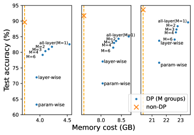
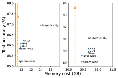
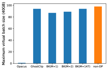
In this context, the all-layer clipping means $M=1$ and another example is the layer-wise or per-layer clipping [27, 7, 18], which treats the parameters (weights and biases) in each layer as one group, hence $M$ equals the number of layers in the neural network. As we will show, the choice of group-wise clipping style has significant influences over the convergence and thus the accuracy (see Figure 1), the computational efficiency, and the algorithmic design (see Figure 2).

Figure 1: Accuracy and memory on CIFAR100 ($\epsilon=2$, virtual batch size 50, left to right: ViT-small/base/large) and QNLI ($\epsilon=3$, virtual batch size 40, left to right: RoBERTa-base/large).

Orthogonal to the per-sample gradient clipping style, a long list of researches have been devoted to efficiently implement the DP optimization, by increasing the training speed and/or reducing the memory cost. One approach is to improve the computational efficiency algorithmically, without affecting the accuracy. For instance, the slowdown of DP optimization (compared to non-DP optimization) has been improved from $24\times$ on small CNN with Tensorflow XLA compiler [32], to $9\times$ in JAX [12], to roughly $2\times$ on GPT2 / RoBERTa / ViT by the ghost clipping technique [22, 6], and finally to $1.1\times$ by the Book-Keeping (BK) technique [10]. In this work, the clipping styles are implemented by the BK algorithm for the best algorithmic efficiency.

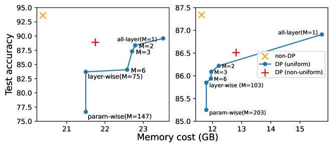
In this work, we study the group-wise clipping style in depth, with a specific emphasis on its convergence and its algorithmic relation to the back-propagation. We observe that the family of group-wise clipping instantiates an accuracy-memory trade-off (i.e. more groups, better memory, worse accuracy), whose two endpoints are the all-layer and layer-wise clipping. In fact, we can group the trainable parameters so as to achieve the best DP accuracy and low memory cost simultaneously (to be demonstrated in Figure 6).

1.1 Contributions

1. [Novel clipping styles] We propose novel choices of the group-wise clipping that are equally fast and private. The uniform clipping is easy to design and instantiates an accuracy-memory trade-off to select; the non-uniform clipping can achieve high accuracy and low memory cost beyond the trade-off, though being harder to design.

2. [A convergence theory] We provide the first convergence result of the group-wise clipping in Theorem 1, showing that DP-SGD has the same asymptotic convergence rate $O(T^{-1/4})$ as the standard SGD, but the convergence guarantee worsens as the number of groups increases.

3. [Guaranteed algorithmic efficiency] We implement our group-wise clipping efficiently so that all group-wise clipping enjoy almost the same training speed as the standard non-DP optimization. This contrasts with prior work which claims that all-layer clipping is about $1.5\sim 2\times$ slower than layer-wise clipping (see [18, Figure 1b]).

4. [Peak memory profile] We provide an explicit memory profile in 6.1, which explains the peak memory of DP optimization and guides the design of group-wise clipping towards larger batch size and faster training.

5. [New baselines] We experiment different choices of group-wise clipping on a range of new DP tasks. We empirically demonstrate that, with the proper group-wise clipping, DP optimization can achieve better accuracy at lower memory cost.

1.2 Related works

Group-wise clipping can be implemented via different algorithms in Tensorflow-privacy, Opacus [35], FastGradClip [21], private-transformer [22]), private-vision [6], FastDP (using BK algorithm [10]). We use BK to implement the group-wise clipping style in Algorithm 1, due to its state-of-the-art efficiency on large-scale vision and language tasks. Notice that, prior to this work, BK algorithms only comes with the all-layer clipping style.

The general concept of group-wise clipping covers a family of gradient clipping styles. The most popular one is the all-layer clipping, which groups all layers into one group and usually enjoys the highest accuracy among other clipping styles. The layer-wise clipping instead groups each layer into a group, thus requiring a long vector of clipping thresholds when the model is of hundreds of layers. These additional hyperparameters $[R_{1},R_{2},...]$ are difficult to tune manually and oftentimes introduce extra privacy risk if tuned adaptively to the data [2, 18]. Similarly, the parameter-wise clipping used by Opacus [35] groups each parameter (weight and bias) into a group. [26] proposes the type-wise clipping such that linear layers form a group and convolution layers form another group. In distributed learning, large models are partitioned into multiple devices, each of which defines a group according to the per-device clipping [18].

Table 1: List of group-wise per-sample gradient clipping styles.

Clipping style	Reference
all-layer	[1]
layer-wise	[27]
param-wise	[35]
type-wise	[26]
per-device	[18]
uniform	this work
non-uniform	this work

In contrast to existing works which focus on specific clipping styles, we explore the whole class of group-wise clipping, thus to reveal an accuracy-memory trade-off. Different from the empirical nature in the literature, we give the first convergence theory of group-wise clipping, and the first peak memory profile from the complexity analysis. We emphasize that the choice of group-wise clipping style can serve as a strong alternative to the adaptive clipping threshold [2, 18].

2 Preliminaries

2.1 Differential privacy in deep learning

We work with the $(\epsilon,\delta)$-DP by [15], where strong DP is indicated by small $(\epsilon,\delta)$ and means it is difficult for any privacy attacker to distinguish or detect an arbitrary training sample.

Definition 2.1 ([15]).

A randomized algorithm $M$ is $(\varepsilon,\delta)$-DP if, for any two neighboring datasets $S,S^{\prime}$ that differ by one data point and for any event $E$,

$$\mathbb{P}[M(S)\in E]\leqslant\mathrm{e}^{\varepsilon}\mathbb{P}\left[M\left(S^{\prime}\right)\in E\right]+\delta.$$ (2)

In deep learning, DP is realized by applying SGD, Adam[19], LAMB[34], FedAvg[25], etc. on the private gradient (1) with respect to the trainable parameters, which are partitioned into $M$ groups and assigned with $M$ clipping thresholds.

We now declare our setting throughout this work:

1. We use automatic (AUTO) clipping function $C_{i}=C(\bm{g}_{i})=\frac{1}{\|\bm{g}_{i}\|_{2}+0.01}$;

2. We use Renyi DP [29] accoutant for all experiments;

3. We use non-adaptive clipping threshold $R_{m}=1/\sqrt{M}$ [27];

4. We use the BK algorithm [10] as our backbone DP implementation.

2.2 Back-propagation

The efficiency of DP optimization is critically determined by that of the per-sample gradient clipping, which can be implemented with marginal overhead by the BK algorithm [10]. Specifically, the BK algorithm makes DP optimization (with the all-layer clipping) almost as efficient as the non-DP optimization, by re-arranging the computation of output gradients and parameter gradients. To see this, we describe two sub-processes of the back-propagation: consider a linear layer (the $l$-th layer), $\bm{a}_{(l+1)}=\phi(\bm{s}_{(l)})=\phi(\bm{a}_{(l)}\mathbf{W}_{(l)}),$ where $\bm{a}\in\mathbb{R}^{BTd}$ is layer’s input (here $B$ being batch size, $T$ being sentence length or number of pixels), $\bm{s}\in\mathbb{R}^{BTp}$ is layer’s output, $\mathbf{W}\in\mathbb{R}^{dp}$ is weight, and $\phi$ is any inter-layer operation like ReLU or pooling.

During the forward propagation, $\bm{a}_{(l)}$ is computed and stored. During the back-propagation, at each layer, the output gradient $\frac{\partial L}{\partial\bm{s}_{(l)}}$ is computed and then produces the parameter gradient:

$$\text{Standard: }\frac{\partial L}{\partial\mathbf{W}_{(l)}}=\frac{\partial\sum_{i}L_{i}}{\partial\mathbf{W}_{(l)}}=\bm{a}_{(l)}^{\top}\frac{\partial L}{\partial\bm{s}_{(l)}}, \text{ DP: }\frac{\partial\sum_{i}C_{i}L_{i}}{\partial\mathbf{W}_{(l)}}=\bm{a}_{(l)}^{\top}\text{diag}(C_{1},\cdots,C_{B})\frac{\partial L}{\partial\bm{s}_{(l)}}.$$ (3)

Here the per-sample gradient norm (or the clipping factor $C_{i}$) can be computed at small cost, i.e. $<10\%$ memory overhead and $\approx 20\%$ slowdown for large models (see Figure 5 in [10]).

2.3 Clipping thresholds

Tuning the clipping threshold vector $\{R_{m}\}\in\mathbb{R}^{M}$ can be expensive for a network with hundreds of layers. The simplest choice is to use the same clipping threshold for all groups [27]: $R_{1}=\cdots=R_{M}=R/\sqrt{M}$. Such a choice is data-independent and model-driven, and we adopt this for the AUTO private gradient: for the $m$-th group,

$$\mathbf{G}_{\text{private}}^{(m)}=\sum_{i}\frac{\bm{g}_{i}^{(m)}}{\sqrt{M}(\|\bm{g}_{i}^{(m)}\|_{2}+0.01)}+\sigma_{\text{DP}}\cdot\mathcal{N}(0,\mathbf{I}_{m}).$$ (4)

It is also possible to use the adaptive data-driven clipping threshold [2, 18, 16], although it needs either extra training data or extra privacy budget. For example, one can use 90% quantile of per-sample gradient norms from the public data as the clipping threshold on the private data, or use a second DP-SGD to learn the adaptive clipping thresholds as hyperparameters, thus adding to the computation cost and privacy budget. Empirically, the benefit of adaptive clipping threshold is insignificant, as illustrated in Table 2.

Table 2: Test accuracy of SST2 dataset at $\epsilon=3$. Results other than ours are from [18].

	Clipping style	10 epochs	20 epochs	30 epochs
RoBERTa-base	all-layer	$90.53$	$90.76$	$91.27$
	layer-wise (adaptive)	$91.30$	$91.57$	$92.10$
	all-layer (ours)	$92.32$	$92.66$	$93.00$
	layer-wise (ours)	$92.09$	$92.43$	$92.55$
RoBERTa-large	all-layer	$93.00$	$93.50$	$93.90$
	layer-wise (adaptive)	$92.80$	$93.63$	$93.67$
	all-layer (ours)	$94.50$	$94.84$	$94.95$
	layer-wise (ours)	$94.15$	$94.27$	$94.38$

3 Algorithm for group-wise clipping

Figure 2: Back-propagation of BK algorithm with the group-wise clipping style.

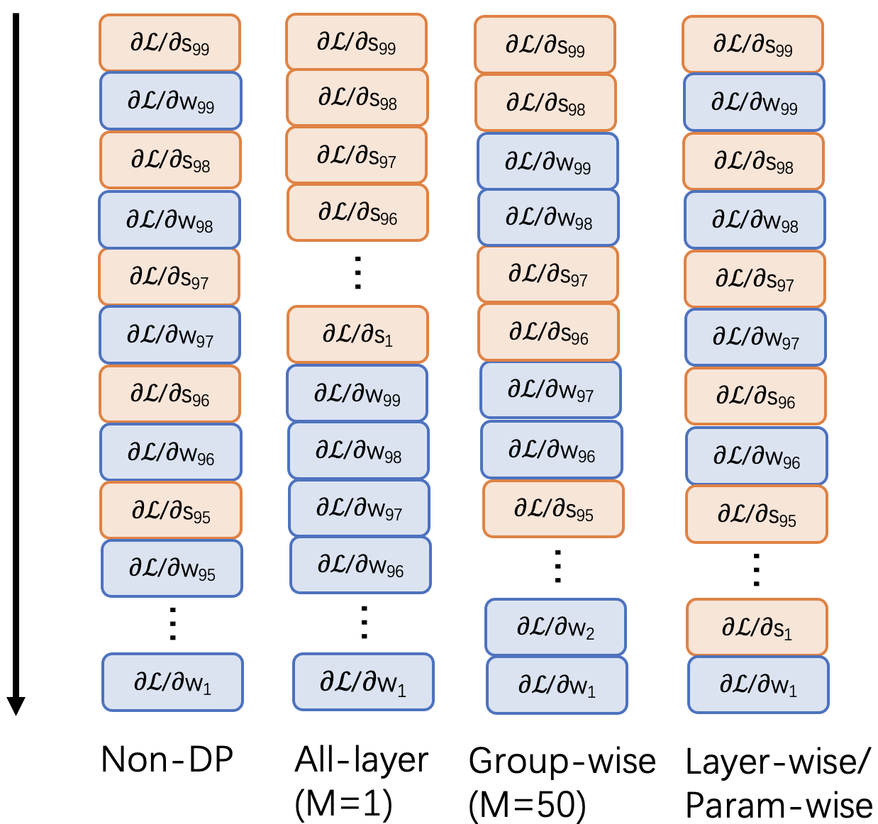
In this section, we modify the back-propagation so as to efficiently implement the group-wise clipping. We note that in (3), to derive the clipping factor $C_{i}$, the output gradients are book-kept until all layers in the current group have been back-propagated. This is visualized in Figure 2 as the stacking of different colors, which represent the computation of output gradients and parameter gradients: consider an 100-layer network and $M=50$, then the group-wise clipping factor $C_{i}$ is computed only if two layers have been back-propagated; when $M=1$ (all-layer clipping), $C_{i}$ is computed after all 100 layers have been back-propagated.

Remark 3.1.

The layer-wise/param-wise clipping does not re-arrange the order of back-propagation (see the similarity of colors in Figure 2). This feature is particularly desirable for distributed learning, where back-propagation involves communication and rewriting the orchestration is hard.

In Algorithm 1, we implement our group-wise clipping in DP optimization, following Figure 2.

Algorithm 1 Differentially private optimization with group-wise clipping

Parameters: $l$-th layer weights $\mathbf{W}_{(l)}$, $m$-th group weights $\mathbf{W}^{(m)}$, noise level $\sigma_{\text{DP}}$.

1:for layer $l=1,2,\cdots$ do

2:     Get activation $\{\bm{a}_{(l)}\}$ by standard forward propagation

3:for layer $l=\cdots,2,1$ do

4:     Get output gradient $\{\frac{\partial L}{\partial\bm{s}_{(l)}}\}$ by standard backward propagation

5:     Compute the layer-wise per-example gradient norm $\|\frac{\partial L_{i}}{\partial\mathbf{W}_{(l)}}\|^{2}$

6:     if $l$ is the first layer of the $m$-th group $\mathcal{G}_{m}$ then

7:         Aggregate gradient norm across layers in this group: $\|\frac{\partial L_{i}}{\partial\mathbf{W}^{(m)}}\|^{2}=\sum_{r\in\mathcal{G}_{m}}\|\frac{\partial L_{i}}{\partial\mathbf{W}_{(r)}}\|^{2}$

8:         Compute group-wise per-sample clipping factor: $C_{i}^{(m)}=1/(\|\frac{\partial L_{i}}{\partial\mathbf{W}^{(m)}}\|+0.01)$

9:         for layer $r\in\mathcal{G}_{m}$ do

10:              Compute sum of clipped gradients $\mathbf{G}_{r}=\sum_{i}\frac{\partial C_{i}^{(m)}L_{i}}{\partial\mathbf{W}_{(r)}}=\bm{a}_{(r)}^{\top}\text{diag}(C_{i}^{(m)})\frac{\partial L}{\partial\bm{s}_{(r)}}$

11:              Delete $\{\bm{a}_{(r)}\},\{\frac{\partial L}{\partial\bm{s}_{(r)}}\}$               

12:Apply SGD/Adam/LAMB with the private gradient $\mathbf{G}_{\text{private}}=\mathbf{G}+\sigma_{\text{DP}}\cdot\mathcal{N}(0,\mathbf{I})$

Figure 3: Accuracy and memory of ViT-large on CIFAR100 ($\epsilon=2$), with uniform group-wise clipping styles. Virtual batch size is 50 except for Opacus, which incurs OOM error (requiring more than 150GB) and at most uses virtual batch size 1 (more than 8 hours per epoch).

In particular, we emphasize that all group-wise clippings have the same time complexity by the BK algorithm, since they only differ in the ordering of computation of output gradients and parameter gradients. This is visualized by the same height in Figure 2 and verified in Figure 3 and Figure 5.

4 Convergence of DP-SGD with group-wise clipping

In this section, we prove the high-probability convergence with any group-wise clipping styles, e.g. layer-wise, parameter-wise, block-wise, all-layer and so on. Our proof only relies on common assumptions in the literature of standard non-DP SGD.

Assumption 4.1 (Lower bound of loss).

For all $\mathbf{w}$, we have $L(\mathbf{w})\geq L_{*}$ for some constant $L_{*}$.

Assumption 4.2 (Smoothness).

Let $\bm{g}(\mathbf{w})$ denote the gradient of the objective $\mathcal{L}(\mathbf{w})$. Then $\forall\mathbf{w},\bm{v}$, there is an non-negative constant $\mathcal{L}$ such that

$$L(\bm{v})-\left[L(\mathbf{w})+\bm{g}(\mathbf{w})^{\top}(\bm{v}-\mathbf{w})\right]\leq\frac{\mathcal{L}}{2}\|\mathbf{w}-\bm{v}\|^{2}$$ (5)

Assumption 4.3 (Gradient noise).

The per-sample gradient noise $\bm{g}_{t,i}^{(m)}-\bm{g}_{t}^{(m)}$ is i.i.d. such that

$$\mathbb{E}(\bm{g}_{t,i}^{(m)}-\bm{g}_{t}^{(m)})=0,\mathbb{E}\|\bm{g}_{t,i}^{(m)}-\bm{g}_{t}^{(m)}\|^{2}\leq\xi^{2}/M,$$

and $\bm{g}_{t,i}^{(m)}$ is symmetric about the oracle gradient $\bm{g}_{t}^{(m)}$: $\bm{g}_{t,i}^{(m)}-\bm{g}_{t}^{(m)}\overset{\mathcal{D}}{=}\bm{g}_{t}^{(m)}-\bm{g}_{t,i}^{(m)}.$

4.1 Effect of number of groups on the convergence

Theorem 1.

Under 4.1, 4.2, 4.3, running DP-SGD with AUTO group-wise clipping (4) for $T$ iterations gives, for arbitrarily small and positive $\varrho$:

$$\max_{t}\mathbb{P}\left(\|\bm{g}_{t}\|<O(\varrho^{-3/2}T^{-1/4})\right)\geq 1-\varrho$$ (6)

where $\bm{g}_{t}=[\bm{g}_{t}^{(1)},\cdots,\bm{g}_{t}^{(M)}]$ and $O(\varrho^{-3/2}T^{-1/4})=(20\xi+\frac{\sqrt{M}}{5})\left(\frac{2M(L_{0}-L_{*})\mathcal{L}\left(1+\frac{\sigma^{2}d}{B^{2}}\right)}{\varrho T}\right)^{\frac{1}{4}}+O\left({\varrho^{-\frac{3}{2}}T^{-\frac{3}{4}}}\right)$. Note that the result for the all-layer clipping corresponds to $M=1$.

In contrast, running the standard (non-DP) SGD for $T$ iterations gives:

$$\max_{t}\mathbb{P}\left(\|\bm{g}_{t}\|<O(\varrho^{-1}T^{-1/4})\right)\geq 1-\varrho.$$ (7)

where $O(\varrho^{-1}T^{-1/4})=\frac{1}{\varrho T^{1/4}}\sqrt{2(L_{0}-L_{*})\mathcal{L}+\frac{\xi^{2}}{B}}$.

We observe in (6) that partitioning trainable parameters into more groups (larger $M$) negatively affects the convergence guarantee. This is empirically verified in Figure 1 and Section 7 across various models. We note, this result does not contradict the fact that the layer-wise clipping uses a finer grouping than the all-layer clipping, as we next explain.

4.2 Finer grouping does not necessarily imply more accurate clipping

Suppose we have two groupings: $\mathcal{G}_{2}$ is finer than $\mathcal{G}_{1}$, in the sense that each group in $\mathcal{G}_{1}$ is partitioned into more groups in $\mathcal{G}_{2}$ (notice that a finer grouping has more groups but the converse does not always hold). It may be tempting to expect that, with the optimal tuning of clipping threshold, the finer grouping is at least as good as the other.

Somewhat surprisingly, we show that this is not the case: it is not true that the group-wise clipping based on $\mathcal{G}_{1}$ is a subset of that based on $\mathcal{G}_{2}$. For instance, the all-layer clipping cannot be viewed as a sub-case of the layer-wise clipping. We prove in Theorem 2 with counter-examples that hold for both Abadi’s and AUTO clipping functions.

Theorem 2.

Consider 2 layers of parameters. There exist per-sample gradients $\bm{g}_{i},\bm{g}_{j}$, such that the all-layer clipping $\mathcal{G}_{1}=\{1,2\}$ cannot be represented as any group-wise clipping $\mathcal{G}_{2}=\{1\},\{2\}$: $\exists R,\forall(R_{1},R_{2})$, at least one of the following holds,

$$\bm{g}_{i}\cdot C(\bm{g}_{i};R_{1},R_{2})\neq\bm{g}_{i}\cdot C(\bm{g}_{i};R)$$

$$\bm{g}_{j}\cdot C(\bm{g}_{j};R_{1},R_{2})\neq\bm{g}_{j}\cdot C(\bm{g}_{j};R)$$

Proof.

We demonstrate with Abadi’s clipping function, though AUTO clipping function can be similarly analyzed. Consider $\bm{g}_{i}=[3,4],\bm{g}_{j}=[6,0]$, and $R=4$. By all-layer clipping, $\langle 1\rangle$ $\bm{g}_{i}$ is clipped, so are its components $\bm{g}_{i}^{(1)},\bm{g}_{i}^{(2)}$; $\langle 2\rangle$ $\bm{g}_{j}$ is not clipped, neither are its components $\bm{g}_{j}^{(1)},\bm{g}_{j}^{(2)}$. No matter how one chooses $R_{1}$, it’s impossible to reproduce the same clipped per-sample gradients: if $R_{1}<\|\bm{g}_{j}^{(1)}\|$, contradicting $\langle 2\rangle$; otherwise, $R_{1}>\|\bm{g}_{j}^{(1)}\|>\|\bm{g}_{i}^{(1)}\|$, contradicting $\langle 1\rangle$. ∎

In fact, we show through the extended proof in appendix that, it is almost impossible in practice that all-layer clipping is a subset of layer-wise clipping. Therefore, one cannot guarantee that the optimal layer-wise clipping (even if adaptively tuned at every iteration) has higher accuracy than the optimal all-layer clipping.

5 Uniform v.s. non-uniform design of grouping

Besides the number of groups, the design of grouping is also critical to the performance of group-wise clipping, although each group-wise clipping is equally $(\epsilon,\delta)$-DP if $\sigma_{\text{DP}}$ is fixed in (1).

Remark 5.1.

The grouping of trainable parameters does not affect the privacy guarantee, because the noise-to-sensitivity ratio is the same [27].

Next, we claim that exhausting all the grouping of layers is computationally infeasible, because the possibilities of grouping is known as the Bell number [3]. This number grows faster than exponentially, with $10^{4.3}$ grouping of 9 layers and $10^{11.8}$ grouping of 18 layers.

Hence, we seek interesting sub-space of the grouping by investigating many factors that justify a good grouping. Existing designs of group-wise clipping, like layer-wise and per-device clipping, are uniform in the sense that each group has roughly the same number of layers or parameters. In Figure 1, we uniformly group the transformer blocks by the common divisor {2,3,4,6} because ViT and RoBERTa have either 12 or 24 blocks.

While the uniform grouping is easy to design, we explore the non-uniform grouping as a broader class that contains uniform ones as special cases, which partitions different number of layers in each group. As we will discuss in Section 6, the non-uniform group-wise clipping can reach beyond the accuracy-memory trade-off of the uniform one.

6 Peak memory profiling

Different grouping has different memory profile, especially in terms of the maximum peak memory in Table 3. As its name suggests, BK algorithm (originally proposed only with all-layer clipping style) book-keeps the output gradients across all layers, which results in a high peak memory. For GPT2 models, DP optimization with all-layer clipping incurs 30% more memory cost than non-DP by [10, Table 8], when the sentence length is long and hence the output gradients are expensive.

Table 3: Accuracy and maximum peak memory of two-group clipping style. Here ‘boundary’ means the first X attention blocks are the first group and the other ($12$-X) blocks are the second group.

	CIFAR100 ViT-large		QNLI RoBERTa-base
boundary	test accuracy	peak memory (GB)	test accuracy	peak memory (GB)
2	88.06	22.04	85.67	11.94
4	88.27	21.96	85.92	11.95
6(uniform)	88.36	21.89	86.22	12.22
8	88.75	21.82	86.38	13.40
10	88.89	21.75	86.29	14.57
all-layer	89.59	23.52	86.91	15.75
non-DP	93.63	20.38	87.34	11.63

For the group-wise clipping style, we can characterize the optimization’s memory profile by the memory peaks: when back-propagation arrives at the first layer of the $m$-th group, at Line 6 in Algorithm 1, all output gradients in this group and all activation tensors in the un-processed groups are cached in the memory. Therefore, $M$ groups lead to $M$ memory peaks, whose form in 6.1 is proved in appendix.

Fact 6.1.

The $m$-th memory peak by space complexity is

$$B(\sum_{l<\mathcal{G}_{m}[-1]}T_{l}d_{l}+\sum_{\mathcal{G}_{m}[0]<r<\mathcal{G}_{m}[-1]}T_{r}p_{r}).$$

Hence, we define the maximum memory peak as

$$B\max_{m}\{\sum_{l<\mathcal{G}_{m}[-1]}T_{l}d_{l}+\sum_{\mathcal{G}_{m}[0]<r<\mathcal{G}_{m}[-1]}T_{r}p_{r}\}$$ (8)

which negatively determines the maximum (virtual) batch size, and thus the maximum throughput (i.e. training speed) of the DP optimization.

6.1 Maximum peak memory of uniform grouping

Figure 4: Space complexity of forward and backward propagation, on top of the memory occupied by data and optimizer states. We use ViT-large-patch16-224 with batch size 32.

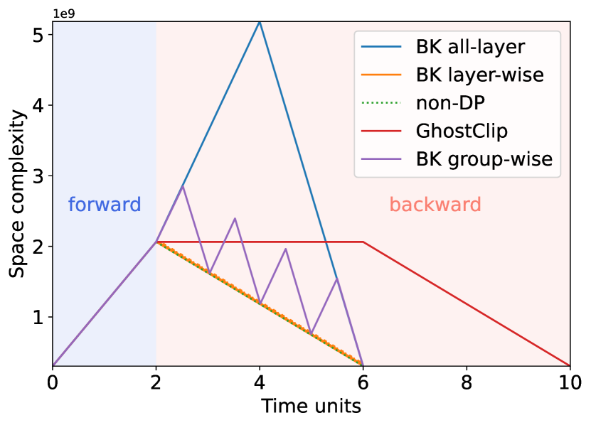
For uniform grouping, the maximum memory peak is always that of the bottom group (the firstly processed during back-propagation), i.e. $m=M$. We visualize the memory peaks of in Figure 4, where the group-wise clipping is $M=4$, and the layer-wise clipping is $M=147$.

We highlight that the maximum peak memory of all-layer clipping occurs when the back-propagation reaches the top layer since all output gradients are book-kept. For layer-wise clipping, the maximum peak memory is similar to that of non-DP training (see also Figure 1), whose peak memory occurs when the back-propagation just starts.

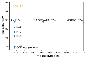
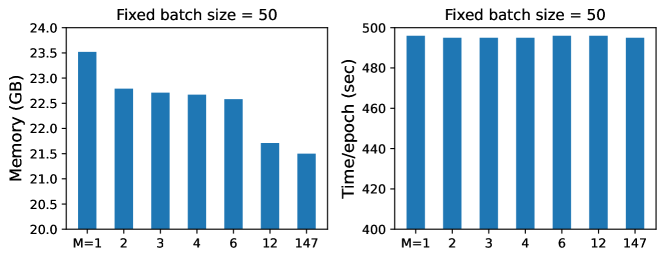
Generally speaking, for uniform grouping, the peak memory increases with smaller number of groups $M$, though the throughput is not affected under BK algorithm (see Figure 5, explained by Section 3).

Figure 5: Peak memory and throughput of ViT-large-patch16-224 using fixed batch size.

6.2 Maximum peak memory of non-uniform grouping

The maximum peak memory of non-uniform grouping can still be described by (8), but not as explicitly as the uniform grouping. For example, with the two-group clipping style, the maximum peak memory may be the first peak or the second one. This explains the non-monotone pattern in Table 3, and motivates to group layers so that the two memory peaks are similar.

Given that the non-uniform grouping contains the uniform grouping as special cases, it usually breaks the accuracy-memory trade-off of the uniform grouping, see Figure 6.

Figure 6: Accuracy and memory on CIFAR100 (ViT-large) and QNLI (RoBERTa-base).

7 Experiments

We experiment the group-wise clipping style on multiple vision and language tasks, in Table 4, Table 5 and Table 7 (in appendix). We focus on the uniform grouping, and cover ViT [14] / RoBERTa [23] / GPT2 [30] models. Empirically speaking, more groups indicate worse accuracy than the all-layer clipping, where the gap decreases as the privacy budget and the model capacity increases. For example, the accuracy gap between layer-wise and all-layer clipping drops from 10% ($\epsilon=2$) to 5% ($\epsilon=8$), when training ViT-small on CIFAR100, and further drops to 2% when training ViT-large. We observe the similar patterns on the text datasets with RoBERTa and GPT2, in which the performance of layer-wise clipping is comparable to that of all-layer clipping. Specially, our results are comparable with the adaptive layer-wise clipping (denoted as $*$ in Table 7 and Table 5) [18], even though they trained 20 epochs on SST2 but we only train 3 epochs.

Table 4: Test accuracy of image classification tasks under group-wise clipping styles.

Model	Method	$\epsilon=2$					$\epsilon=8$
		CIFAR10	CIFAR100	SVHN	GTSRB	Food101	CIFAR10	CIFAR100	SVHN	GTSRB	Food101
ViT -small	all-layer $(M=1)$	96.94	82.58	91.28	89.57	73.45	97.13	85.00	92.92	94.55	77.12
	non-uniform $(M=2)$	97.01	82.68	90.77	89.70	74.45	97.11	85.23	92.24	94.77	78.14
	uniform $(M=2)$	96.87	81.79	91.39	89.55	72.48	97.00	84.45	92.98	94.59	76.68
	uniform $(M=3)$	96.81	80.96	91.02	89.55	71.97	96.99	84.36	92.71	94.70	76.37
	uniform $(M=4)$	96.81	80.45	90.95	89.70	71.47	96.96	84.09	92.52	94.66	76.14
	uniform $(M=6)$	96.72	79.24	90.96	89.89	70.88	96.93	83.49	92.44	94.67	75.76
	layer-wise $(M=75)$	96.60	71.93	90.42	87.18	65.21	96.86	80.49	91.87	93.88	71.96
	param-wise $(M=150)$	96.34	63.24	89.04	80.77	59.42	96.71	75.09	90.90	91.91	67.85
ViT -large	all-layer $(M=1)$	98.68	89.59	93.27	91.81	82.29	98.92	90.66	94.26	95.68	84.84
	non-uniform $(M=2)$	98.60	88.89	93.14	91.61	81.46	98.90	90.36	94.16	95.70	84.39
	uniform $(M=2)$	98.52	88.36	92.77	90.89	81.13	98.69	90.36	93.79	95.27	84.05
	uniform $(M=3)$	98.59	87.31	92.42	90.31	79.68	98.71	89.95	93.59	95.17	83.33
	uniform $(M=4)$	98.51	86.38	92.31	89.97	78.46	98.70	89.48	93.34	94.88	82.61
	uniform $(M=6)$	98.56	84.08	92.16	88.99	76.66	98.66	88.89	93.19	94.73	81.59
	layer-wise $(M=147)$	98.37	83.70	92.61	89.87	77.89	98.57	88.65	93.79	94.62	82.68
	param-wise $(M=294)$	98.24	76.66	91.48	85.28	72.59	98.47	86.43	93.14	92.73	79.61

Table 5: Test score of text generation on E2E dataset under group-wise clipping styles.

Model	Method		$\epsilon=3$					$\epsilon=8$
			BLEU	ROGUE-L	NIST	METEOR	CIDEr	BLE	ROGUE-L	NIST	METEOR	CIDEr
GPT2 -small	RGP	[37]	58.48	65.56	5.775	0.331	1.300	58.46	65.03	6.276	0.349	1.496
	all-layer $(M=1)$	[22]	61.52	65.67	6.697	0.384	1.761	63.19	66.43	7.444	0.400	1.919
	all-layer $(M=1)$	[9]	61.34	65.87	7.071	0.387	1.801	63.60	67.07	7.714	0.404	1.938
	block-wise $(M=12)$	ours	61.03	66.07	6.863	0.388	1.787	63.65	67.36	7.773	0.406	1.951
	layer-wise $(M=76)$	ours	60.76	65.93	6.680	0.386	1.766	63.47	67.49	7.791	0.407	1.975
	layer-wise $(M=76)$	[18]	61.10	65.12	-	-	-	63.42	66.69	-	-	-
	param-wise $(M=149)$	ours	57.97	64.84	6.002	0.372	1.624	62.07	66.27	7.197	0.393	1.848
GPT2 -medium	all-layer $(M=1)$	[9]	63.85	67.07	7.106	0.387	1.754	64.22	67.53	8.172	0.418	2.081
	block-wise $(M=24)$	ours	61.43	66.93	7.998	0.411	2.009	64.07	68.18	8.332	0.429	2.230
	layer-wise $(M=148)$	ours	61.80	66.76	7.865	0.407	1.974	63.96	68.44	8.325	0.429	2.237
	param-wise $(M=293)$	ours	60.48	64.95	6.981	0.391	1.804	62.50	67.28	8.178	0.419	2.098
GPT2 -large	all-layer $(M=1)$	[9]	64.18	67.86	7.937	0.403	2.008	64.64	68.97	8.301	0.420	2.163
	block-wise $(M=36)$	ours	65.23	69.04	8.467	0.435	2.234	66.90	69.87	8.548	0.444	2.355
	layer-wise $(M=220)$	ours	64.86	68.30	8.417	0.431	2.219	66.44	69.55	8.504	0.443	2.297
	param-wise $(M=437)$	ours	63.85	67.83	8.303	0.416	2.093	65.01	68.79	8.429	0.435	2.238

8 Discussion

We show that group-wise clipping, a superset that covers existing clipping styles, leads to different accuracy and efficiency depending on the grouping of trainable parameters. For accuracy, a small number of groups (e.g. the all-layer clipping) benefits the convergence, though the accuracy gap among different group-wise clippings is negligible for larger models. For time efficiency, all group-wise clippings are equally fast under the most efficient BK algorithm. For memory efficiency, the uniform group-wise clipping with more groups has smaller peak memory and thus form an accuracy-memory trade-off. However, the non-uniform grouping can reach beyond this trade-off with a careful design.

Overall, a proper group-wise clipping style makes system design easy and allows large DP models to be accurate, fast to train, and memory-efficient. This finally closes the accuracy and efficiency gap between DP and standard non-DP models, thus allowing us to establish new state-of-the-art results on multiple datasets, without relying on adaptive clipping or longer training epochs. For future work, more exploration of the grouping is desirable, especially in the orthogonal direction of parameter-efficient fine-tuning [36, 28, 8].

Appendix A Proofs

A.1 Proof of Theorem 2

Proof.

(Proof for Abadi’s clipping) Consider a two-layer neural network and two per-sample gradients $\bm{g}_{1}=[\bm{g}_{1}^{(1)},\bm{g}_{1}^{(2)}],\bm{g}_{2}=[\bm{g}_{2}^{(1)},\bm{g}_{2}^{(2)}]$. Suppose $\|\bm{g}_{1}^{(1)}\|<\|\bm{g}_{2}^{(1)}\|$ and $\|\bm{g}_{1}\|>R>\|\bm{g}_{2}\|$. Then in the all-layer clipping, the first per-sample gradient $\bm{g}_{1}$ is clipped/scaled, and so are both its components $\bm{g}_{1}^{(1)},\bm{g}_{1}^{(2)}$. But the second per-sample gradient $\bm{g}_{2}$ is not clipped. However, in the layer-wise clipping with any choice of $\bm{R}=(R_{1},R_{2})$, there are two cases both leading to the contradiction.

1. $R_{1}<\|\bm{g}_{2}^{(1)}\|$. Then $\bm{g}_{2}^{(1)}$ is clipped by layer-wise. But $\bm{g}_{2}^{(1)}$ is not clipped by all-layer. Done.

2. $R_{1}>\|\bm{g}_{2}^{(1)}\|$. Then $\bm{g}_{2}^{(1)}$ is not clipped by layer-wise, and so is not $\bm{g}_{1}^{(1)}$ since $\|\bm{g}_{1}^{(1)}\|<\|\bm{g}_{2}^{(1)}\|$. But $\bm{g}_{1}^{(1)}$ is clipped by all-layer. Done.

In fact, we can generalize this non-equivalence between the all-layer and layer-wise clipping: for small $R$ (say $R<\|\bm{g}_{i}\|$), a necessary (but impossible) condition to claim that, the all-layer clipping is a sub-case of the layer-wise clipping, would be

$$\frac{\|\bm{g}_{i}^{(m)}\|}{\|\bm{g}_{i}\|}=\frac{\|\bm{g}_{j}^{(m)}\|}{\|\bm{g}_{j}\|},\forall i,j\in[B],m\in[M].$$

Here $B$ is the batch size and $M$ is the number of groups.

(Proof for automatic clipping) Here we work with the $R$-dependent automatic clipping, which is mathematically equivalent to the automatic clipping in (4), according to Theorem 1& 2 in [9]. We consider a $M$-group neural network and per-sample gradients $\bm{g}_{i}$. Suppose the layer-wise clipping can represent the all-layer clipping with $R$, then

$$\frac{R_{m}\bm{g}_{i}^{(m)}}{\|\bm{g}_{i}^{(m)}\|+0.01}=\frac{R\bm{g}_{i}^{(m)}}{\|\bm{g}_{i}\|+0.01},\forall i\in[B],m\in[M].$$

This requires that

$$\frac{\|\bm{g}_{i}^{(m)}\|+0.01}{\|\bm{g}_{i}\|+0.01}=\frac{\|\bm{g}_{j}^{(m)}\|+0.01}{\|\bm{g}_{j}\|+0.01},\forall i,j\in[B],m\in[M],$$

which is practically impossible to hold. ∎

A.2 Proof of Theorem 1: DP-SGD

Proof.

Consider DP-SGD with the automatic (AUTO-S [9]) clipping in a layer-wise style, i.e. $\gamma=0.01$.

$$\mathbf{w}_{t+1}^{(m)}=\mathbf{w}_{t}^{(m)}-\eta\left(\frac{\sum_{i}\bm{g}^{(m)}_{t,i}/(\|\bm{g}^{(m)}_{t,i}\|+\gamma)}{\sqrt{M}}+\sigma\mathcal{N}(0,\mathbf{I})\right)$$

where $\bm{g}^{(m)}_{t,i}$ is i.i.d. unbiased estimate of $\bm{g}^{(m)}_{t}$, with a bounded variance as described in 4.3.

By the Lipschitz smoothness in 4.2,

$$L_{t+1}-L_{t}\leq\sum_{m}\left[\bm{g}^{(m)\top}_{t}(\mathbf{w}_{t+1}^{(m)}-\mathbf{w}^{(m)}_{t})\right]+\frac{\mathcal{L}}{2}\sum_{m}\|\mathbf{w}^{(m)}_{t+1}-\mathbf{w}^{(m)}_{t}\|^{2}$$

$$=-\eta\sum_{m}\left[\bm{g}^{(m)\top}_{t}\left(\sum_{i}\frac{\bm{g}^{(m)}_{t,i}}{\sqrt{M}(\|\bm{g}^{(m)}_{t,i}\|+\gamma)}+\sigma\mathcal{N}(0,I)\right)\right]+\frac{\mathcal{L}\eta^{2}}{2}\sum_{m}\left\|\sum_{i}\frac{\bm{g}^{(m)}_{t,i}}{\sqrt{M}(\|\bm{g}^{(m)}_{t,i}\|+\gamma)}+\sigma\cdot\mathcal{N}(0,\mathbf{I})\right\|^{2}$$

Given the fact that $\left\|\frac{\bm{g}^{(m)}_{t,i}}{\|\bm{g}^{(m)}_{t,i}\|+\gamma}\right\|\leq 1$, we expand the square of norm and the expected improvement at one iteration is

$$\begin{split}\mathbb{E}(L_{t+1}-L_{t}|\mathbf{w}_{t})&\leq-\frac{\eta}{\sqrt{M}}\sum_{m}\bm{g}^{(m)\top}_{t}\mathbb{E}\left(\sum_{i}\frac{\bm{g}_{t,i}^{(m)}}{\|\bm{g}_{t,i}^{(m)}\|+\gamma}\right)+\frac{\mathcal{L}\eta^{2}}{2}\sum_{m}\left(\frac{1}{M}\mathbb{E}\left\|\sum_{i}\frac{\bm{g}_{t,i}^{(m)}}{||\bm{g}_{t,i}^{(m)}||+\gamma}\right\|^{2}+\sigma^{2}d^{(m)}\right)\\ &\leq-\frac{B\eta}{\sqrt{M}}\sum_{m}\bm{g}^{(m)\top}_{t}\mathbb{E}\left(\frac{\bm{g}_{t,i}^{(m)}}{\|\bm{g}_{t,i}^{(m)}\|+\gamma}\right)+\frac{\mathcal{L}\eta^{2}}{2}\sum_{m}\left(\frac{B^{2}}{M}+\sigma^{2}d^{(m)}\right)\end{split}$$ (9)

in which $d^{(m)}$ is the number of parameters in the $m$-th group and $d=\sum_{m}d^{(m)}$ is the total number of model parameters.

Now we can lower bound $\bm{g}_{t}^{(m)\top}\mathbb{E}\left(\frac{\bm{g}^{(m)}_{t,i}}{\|\bm{g}^{(m)}_{t,i}\|+\gamma}\right)$ in (9) by Lemma A.1.

Lemma A.1.

Denoting $\|\bm{g}^{(m)}_{t}\|-\frac{\xi}{r\sqrt{M}}$ as $x_{r}$, then for any $r>1$ we have

$$\bm{g}_{t}^{(m)\top}\mathbb{E}\left(\frac{\bm{g}^{(m)}_{t,i}}{\|\bm{g}^{(m)}_{t,i}\|+\gamma}\right)\geq\frac{1}{2}\cdot\underbrace{x_{r}\left(\frac{\gamma}{(r-1)(x_{r}+\frac{\xi}{r\sqrt{M}})+\gamma}-\frac{\gamma}{(r+1)(x_{r}+\frac{\xi}{r\sqrt{M}})+\gamma}\right)}_{\mathcal{M}(x_{r};r,\xi,\gamma)}$$ (10)

Here $\mathcal{M}$ is non-negative and strictly increasing, with $\mathcal{M}(0)=0$. Thus $\mathcal{M}$ can be viewed as a distance measure.

Using this lower bound, the expected improvement (9) becomes

$$\mathbb{E}(L_{t+1}-L_{t}|\mathbf{w}_{t}) \leq-\frac{B\eta}{2\sqrt{M}}\sum_{m}\left[\mathcal{M}(\|\bm{g}^{(m)}_{t}\|-\frac{\xi}{r\sqrt{M}})\right]+\frac{\mathcal{L}\eta^{2}}{2}\left(B^{2}+\sigma^{2}d\right)$$

Now extend the expectation over randomness in the trajectory, and perform a telescoping sum over the iterations

$$L_{0}-L_{*} \geq L_{0}-\mathbb{E}L_{T}=\sum_{t}\mathbb{E}(L_{t}-L_{t+1})$$

$$\geq\frac{B\eta}{2\sqrt{M}}\mathbb{E}\left(\sum_{t,m}\mathcal{M}(\|\bm{g}^{(m)}_{t}\|-\frac{\xi}{r\sqrt{M}})\right)-\frac{T\mathcal{L}\eta^{2}}{2}\left(B^{2}+\sigma^{2}d\right)$$

Substituting $\eta B=\eta_{\text{0}}/\sqrt{T}$ where $\eta_{\text{0}}$ is a base learning rate, we have

$$2(L_{0}-L_{*})\geq\sqrt{\frac{T}{M}}\eta_{\text{0}}\mathbb{E}\left(\frac{1}{T}\sum_{t,m}\mathcal{M}(\|\bm{g}^{(m)}_{t}\|-\frac{\xi}{r\sqrt{M}})\right)-\mathcal{L}\eta^{2}_{\text{0}}\left(1+\frac{\sigma^{2}d}{B^{2}}\right)$$

and finally

$$\mathbb{E}\left(\frac{1}{T}\sum_{t,m}\mathcal{M}(\|\bm{g}^{(m)}_{t}\|-\frac{\xi}{r\sqrt{M}})\right)\leq\sqrt{\frac{M}{T}}\left[\frac{2(L_{0}-L_{*})}{\eta_{\text{0}}}+\mathcal{L}\eta_{\text{0}}\left(1+\frac{\sigma^{2}d}{B^{2}}\right)\right]$$ (11)

With $\eta_{\text{0}}$ chosen properly as $\sqrt{\frac{2(L_{0}-L_{*})}{\mathcal{L}(1+\frac{\sigma^{2}d}{B^{2}})}}$, the hyperbola on the right hand side in (11) is minimized to $2\sqrt{\frac{M}{T}}\sqrt{2(L_{0}-L_{*})\mathcal{L}\left(1+\frac{\sigma^{2}d}{B^{2}}\right)}$.

Since the minimum of a sequence is smaller than the average, we have

$$\min_{t}\mathbb{E}(\sum_{m}\mathcal{M}(\|\bm{g}^{(m)}_{t}\|-\frac{\xi}{r\sqrt{M}}))\leq 2\sqrt{\frac{M}{T}}\sqrt{2(L_{0}-L_{*})\mathcal{L}\left(1+\frac{\sigma^{2}d}{B^{2}}\right)}$$ (12)

Then by the Markov’s inequality (since $\mathcal{M}$ is non-negative), for any constant $a>0$,

$$\min_{t}\sum_{m}\mathbb{P}(\mathcal{M}(\|\bm{g}^{(m)}_{t}\|-\frac{\xi}{r\sqrt{M}})>a)\leq\frac{2}{a}\sqrt{\frac{M}{T}}\sqrt{2(L_{0}-L_{*})\mathcal{L}\left(1+\frac{\sigma^{2}d}{B^{2}}\right)}$$ (13)

Note that

$$\sum_{m}\mathbb{P}\left(\mathcal{M}(\|\bm{g}^{(m)}_{t}\|-\frac{\xi}{r\sqrt{M}})>a\right)>1-\mathbb{P}\left(\bigcap_{m}\mathcal{M}(\|\bm{g}^{(m)}_{t}\|-\frac{\xi}{r\sqrt{M}})<a\right)$$

which leads Equation 13 to

$$\max_{t}\mathbb{P}\left(\bigcap_{m}\mathcal{M}(\|\bm{g}^{(m)}_{t}\|-\frac{\xi}{r\sqrt{M}})<a\right)\geq 1-\frac{2\sqrt{M}}{a\sqrt{T}}\sqrt{2(L_{0}-L_{*})\mathcal{L}\left(1+\frac{\sigma^{2}d}{B^{2}}\right)}$$ (14)

Denoting the inverse function of $\mathcal{M}$ as $\mathcal{M}^{-1}$, whose explicit formula will be given in Lemma A.2, we get

$$\max_{t}\mathbb{P}\left(\bigcap_{m}\|\bm{g}^{(m)}_{t}\|^{2}<\big{(}\mathcal{M}^{-1}(a)+\frac{\xi}{r\sqrt{M}}\big{)}^{2}\right)\geq 1-\frac{2\sqrt{M}}{a\sqrt{T}}\sqrt{2(L_{0}-L_{*})\mathcal{L}\left(1+\frac{\sigma^{2}d}{B^{2}}\right)}$$ (15)

It is obvious that $\|\bm{g}^{(m)}_{t}\|$ being small for all $1\leq m\leq M$ is a sufficient condition to guarantee $\|\bm{g}_{t}\|$ to be small. Therefore,

$$\mathbb{P}\left(\|\bm{g}_{t}\|<\sqrt{M}\big{(}\mathcal{M}^{-1}(a)+\frac{\xi}{r\sqrt{M}}\big{)}\right) \geq\mathbb{P}\left(\bigcap_{m}\|\bm{g}^{(m)}_{t}\|^{2}<\big{(}\mathcal{M}^{-1}(a)+\frac{\xi}{r\sqrt{M}}\big{)}^{2}\right)$$

and consequently we have the high probability bound for any $r>1,a>0$:

$$\max_{t}\mathbb{P}\left(\|\bm{g}_{t}\|<\sqrt{M}\mathcal{M}^{-1}(a;r,\xi,\gamma)+\frac{\xi}{r}\right)\geq 1-\frac{2\sqrt{M}}{a\sqrt{T}}\sqrt{2(L_{0}-L_{*})\mathcal{L}\left(1+\frac{\sigma^{2}d}{B^{2}}\right)}.$$ (16)

In order for $\|\bm{g}_{t}\|$ to converge to zero, we need both $\mathcal{M}^{-1}(a)\to 0$ and $\frac{\xi}{r}\to 0$, as $T\to\infty$. I.e. we consider $a\to 0$. We use Lemma A.2 to claim that, under any fixed $r$,

$$\sqrt{M}\mathcal{M}^{-1}(a)+\frac{\xi}{r} =r\cdot\frac{aM(\frac{\xi}{\sqrt{M}}+\gamma)^{2}}{2\xi\gamma}+\frac{1}{r}\cdot\left(\xi-\frac{a\xi}{2\gamma}\right)+o(a)$$

so that

$$\min_{r}\sqrt{M}\mathcal{M}^{-1}(a)+\frac{\xi}{r} =2\sqrt{\frac{aM(\frac{\xi}{\sqrt{M}}+\gamma)^{2}}{2\xi\gamma}\cdot\left(\xi-\frac{a\xi}{2\gamma}\right)}+o(a)$$

where the last equality is obvious for a hyperbola with respect to $r$. In fact, the square root term simplifies to $\sqrt{2a(\xi+\gamma\sqrt{M})^{2}/\gamma}+O(a^{1.5})$, and so does the whole term. To put this into perspective, we denote $\varrho:=\frac{2\sqrt{M}}{a\sqrt{T}}\sqrt{2(L_{0}-L_{*})\mathcal{L}\left(1+\frac{\sigma^{2}d}{B^{2}}\right)}$. Then we can write Equation 16 asymptotically

$$\max_{t}\mathbb{P}\left(\|\bm{g}_{t}\|<\sqrt{2a(\xi+\gamma\sqrt{M})^{2}/\gamma}+O(a^{1.5})\right)\geq 1-\varrho.$$

which becomes

$$\max_{t}\mathbb{P}\left(\|\bm{g}_{t}\|<2(\xi+\gamma\sqrt{M})\sqrt{\frac{\sqrt{M}}{\varrho\gamma}\sqrt{\frac{2(L_{0}-L_{*})\mathcal{L}\left(1+\frac{\sigma^{2}d}{B^{2}}\right)}{T}}}+O\left(\frac{1}{\varrho^{1.5}T^{0.75}}\right)\right)\geq 1-\varrho.$$

∎

Lemma A.2.

The explicit form of $\mathcal{M}^{-1}$ is

$$\mathcal{M}^{-1}(x;r,\xi,\gamma)=\frac{-\frac{\xi}{r\sqrt{M}}\gamma+(r^{2}-1)\frac{\xi}{r\sqrt{M}}x+r\gamma x+\gamma\sqrt{(\frac{\xi}{r\sqrt{M}})^{2}+2\frac{\xi}{\sqrt{M}}x+2\gamma x+x^{2}}}{2\gamma-(r^{2}-1)x},$$ (17)

and the asymptotic form (as $x\to 0$) is linear:

$$\mathcal{M}^{-1}(x;r,\xi,\gamma)=x\cdot\frac{r^{2}(\frac{\xi}{\sqrt{M}}+\gamma)^{2}-(\frac{\xi}{\sqrt{M}})^{2}}{2\frac{\xi}{\sqrt{M}}\gamma r}+o(x),$$ (18)

Proof of Lemma A.2.

The explicit form of $\mathcal{M}^{-1}$ can be easily verified by $\mathcal{M}^{-1}(\mathcal{M}(x))=x$. In fact, this has already been shown in [9] where $M=1$ (i.e. we switch $\xi$ to $\xi/\sqrt{M}$). One can also check this using Equation 10 and WolframAlpha by searching

inverse function cx/((r-1)(x+a)+c)-cx/((r+1)(x+a)+c)

where c means $\gamma$, a means $\frac{\xi}{r\sqrt{M}}$, and r means $r$.

The asymptotic form of $\mathcal{M}^{-1}$ can be derived from the asymptotic form of $\mathcal{M}$ in Equation 10:

$$\mathcal{M}(x)=x\left(\frac{\gamma}{(r-1)\frac{\xi}{r\sqrt{M}}+\gamma}-\frac{\gamma}{(r+1)\frac{\xi}{r\sqrt{M}}+\gamma}\right)+O(x^{2})=\frac{2\frac{\xi}{\sqrt{M}}\gamma rx}{r^{2}(\frac{\xi}{\sqrt{M}}+\gamma)^{2}-(\frac{\xi}{\sqrt{M}})^{2}}+O(x^{2}).$$

This can be checked by WolframAlpha through

x(c/((r-1)(x+a)+c)-c/((r+1)(x+a)+c)) expand x=0

Therefore, we have

$$\mathcal{M}^{-1}(x)=x\cdot\frac{r^{2}(\frac{\xi}{\sqrt{M}}+\gamma)^{2}-(\frac{\xi}{\sqrt{M}})^{2}}{2\frac{\xi}{\sqrt{M}}\gamma r}+O(x^{2}).$$

∎

A.3 Proof of Theorem 1: standard SGD

Proof.

This proof is similar to Theorem 4 in [9], though theirs is of expected convergence and ours is of high probability. Consider standard (non-DP) SGD,

$$\mathbf{w}^{(m)}_{t+1}=\mathbf{w}^{(m)}_{t}-\eta\frac{\sum_{i}\bm{g}^{(m)}_{t,i}}{B}$$

where $\bm{g}^{(m)}_{t,i}$ is i.i.d. unbiased estimate of $\bm{g}^{(m)}_{t}$ with a bounded variance in 4.3.

By Lipschitz smoothness in 4.2,

$$L_{t+1}-L_{t}\leq\sum_{m}\left[\bm{g}^{(m)\top}_{t}(\mathbf{w}^{(m)}_{t+1}-\mathbf{w}^{(m)}_{t})\right]+\frac{\mathcal{L}}{2}\sum_{m}\|\mathbf{w}^{(m)}_{t+1}-\mathbf{w}^{(m)}_{t}\|^{2}$$

$$=-\eta\sum_{m}\left[\bm{g}^{(m)\top}_{t}\left(\sum_{i}\frac{\bm{g}^{(m)}_{t,i}}{B}\right)\right]+\frac{\mathcal{L}\eta^{2}}{2}\sum_{m}\left\|\sum_{i}\frac{\bm{g}^{(m)}_{t,i}}{B}\right\|^{2}.$$

The expected improvement at one iteration is

$$\begin{split}\mathbb{E}(L_{t+1}-L_{t}|\mathbf{w}_{t})&\leq-\eta\sum_{m}\bm{g}^{(m)\top}_{t}\mathbb{E}\left(\bm{g}^{(m)}_{t,i}\right)+\frac{\mathcal{L}\eta^{2}}{2}\sum_{m}\mathbb{E}\left(\|\sum_{i}\frac{\bm{g}^{(m)}_{t,i}}{B}\|^{2}\right)\\ &\leq-\eta\sum_{m}\bm{g}^{(m)\top}_{t}\bm{g}^{(m)}_{t}+\frac{\mathcal{L}\eta^{2}}{2}\sum_{m}(\|\bm{g}^{(m)}_{t}\|^{2}+\frac{\xi^{2}}{LB})\\ &=-\eta\|\bm{g}_{t}\|^{2}+\frac{\mathcal{L}\eta^{2}}{2}(\|\bm{g}_{t}\|^{2}+\frac{\xi^{2}}{B})\end{split}$$ (19)

Notice that Equation 19 does not require the symmetry assumption in 4.3 for the per-sample gradient noise. We extend the expectation over randomness in the trajectory, and perform a telescoping sum,

$$L_{0}-L_{*} \geq\sum_{t}\mathbb{E}(L_{t}-L_{t+1})\geq\left(\eta-\frac{\mathcal{L}\eta^{2}}{2}\right)\mathbb{E}(\sum_{t}\|\bm{g}_{t}\|^{2})-\frac{T\mathcal{L}\eta^{2}\xi^{2}}{2B}$$

We apply the same learning rate as in [4] and [9], namely $\eta=1/\mathcal{L}\sqrt{T}$, to get

$$L_{0}-L_{*}\geq\left(\frac{1}{\mathcal{L}\sqrt{T}}-\frac{1}{2\mathcal{L}T}\right)\mathbb{E}\left(\sum_{t}\|\bm{g}_{t}\|^{2}\right)-\frac{\xi^{2}}{2B\mathcal{L}}>\frac{\sqrt{T}}{2\mathcal{L}}\mathbb{E}\left(\frac{1}{T}\sum_{t}\|\bm{g}_{t}\|^{2}\right)-\frac{\xi^{2}}{2B\mathcal{L}}$$

and thus

$$\min_{t}\mathbb{E}\left(\|\bm{g}_{t}\|^{2}\right)\leq\frac{1}{T}\sum_{t}\mathbb{E}\left(\|\bm{g}_{t}\|^{2}\right)=\mathbb{E}\left(\frac{1}{T}\sum_{t}\|\bm{g}_{t}\|^{2}\right)\leq\frac{1}{\sqrt{T}}\left[2(L_{0}-L_{*})\mathcal{L}+\frac{\xi^{2}}{B}\right]$$

Using the Jensen’s inequality and the Markov’s inequality, we can have

$$\min_{t}a\cdot\mathbb{P}(\|\bm{g}_{t}\|>a)\leq\min_{t}\mathbb{E}\left(\|\bm{g}_{t}\|\right)\leq\min_{t}\sqrt{\mathbb{E}\left(\|\bm{g}_{t}\|^{2}\right)}\leq\frac{1}{T^{1/4}}\sqrt{2(L_{0}-L_{*})\mathcal{L}+\frac{\xi^{2}}{B}}$$

for any positive constant $a$. Denoting $a=\frac{1}{T^{1/4}}\sqrt{2(L_{0}-L_{*})\mathcal{L}+\frac{\xi^{2}}{B}}/\varrho$, we have

$$\max_{t}\mathbb{P}\left(\|\bm{g}_{t}\|<\frac{1}{\varrho T^{1/4}}\sqrt{2(L_{0}-L_{*})\mathcal{L}+\frac{\xi^{2}}{B}}\right)\geq 1-\varrho.$$

∎

Appendix B Experiment settings

All experiments are fully fine-tuned using a single Nvidia A100 GPU.

Dataset	CIFAR/SVHN/Food101	GTSRB	MNLI(m/mm)	QQP	QNLI	SST2	E2E
Model	ViT		RoBERTa				GPT2
Epoch	5	10	18	18	6	3	10
Batch size	1000	1000	12000	12000	4000	2000	1000
DP learning rate	5e-4	5e-4	3e-4	3e-4	3e-4	3e-4	1e-3
learning rate schedule	—	—	—	—	—	—	—
AdamW weight decay	0.01	0.01	0	0	0	0	0.01
Hidden feature dimension	224*224	224*224	256	256	256	256	100

Table 6: Hyperparameters for Table 4, Table 7, and Table 5. Note that we use automatic clipping which need not to set the clipping threshold.

Appendix C Extra experiments

Table 7: Test accuracy of text classification tasks under group-wise clipping styles.

Model	Method		$\epsilon=3$				$\epsilon=8$
			MNLI	QQP	QNLI	SST2	MNLI	QQP	QNLI	SST2
RoBERTa -base	RGP	[37]	-/-	-	-	-	80.5/-	85.5	87.2	91.6
	all-layer $(M=1)$	[22]	82.45/82.99	85.56	87.42	91.86	83.20/83.46	86.08	87.94	92.09
	all-layer $(M=1)$	[9]	83.22/83.21	85.76	86.91	92.32	83.82/83.55	86.58	87.85	92.43
	block-wise $(M=12)$	ours	82.55/83.19	84.14	85.94	91.74	83.06/83.29	84.73	86.40	91.97
	layer-wise $(M=103)$	ours	82.02/82.56	83.26	85.85	91.40	82.24/82.84	83.49	86.42	92.09
	layer-wise* $(M=103)$	[18]	82.83/83.27	85.67	86.13	92.03	83.70/83.97	86.23	87.13	92.40
	param-wise $(M=203)$	ours	81.63/82.10	82.52	85.25	91.28	82.22/82.49	82.80	86.09	91.63
RoBERTa -large	RGP	[37]	-/-	-	-	-	86.1/-	86.7	90.0	93.0
	all-layer $(M=1)$	[22]	86.43/86.46	86.43	90.76	93.04	87.02/87.26	87.47	91.10	93.81
	all-layer $(M=1)$	[9]	86.27/86.67	86.7	91.01	93.92	87.07/87.16	87.47	91.45	94.61
	block-wise $(M=24)$	ours	87.26/87.28	85.81	89.86	94.15	87.54/87.29	86.55	90.78	94.61
	layer-wise $(M=199)$	ours	86.37/86.66	84.78	89.60	94.38	86.53/86.93	85.22	90.10	94.50
	layer-wise* $(M=199)$	[18]	87.10/87.20	86.80	89.80	93.87	87.67/87.57	87.20	90.77	94.03
	param-wise $(M=395)$	ours	86.47/86.38	84.49	89.11	93.72	86.43/86.39	85.17	89.84	94.27

References

- [1] Martin Abadi, Andy Chu, Ian Goodfellow, H Brendan McMahan, Ilya Mironov, Kunal Talwar, and Li Zhang. Deep learning with differential privacy. In Proceedings of the 2016 ACM SIGSAC conference on computer and communications security, pages 308–318, 2016.
- [2] Galen Andrew, Om Thakkar, Brendan McMahan, and Swaroop Ramaswamy. Differentially private learning with adaptive clipping. Advances in Neural Information Processing Systems, 34:17455–17466, 2021.
- [3] Eric Temple Bell. The iterated exponential integers. Annals of Mathematics, pages 539–557, 1938.
- [4] Jeremy Bernstein, Yu-Xiang Wang, Kamyar Azizzadenesheli, and Animashree Anandkumar. signsgd: Compressed optimisation for non-convex problems. In International Conference on Machine Learning, pages 560–569. PMLR, 2018.
- [5] Zhiqi Bu, Jinshuo Dong, Qi Long, and Weijie J Su. Deep learning with gaussian differential privacy. Harvard data science review, 2020(23), 2020.
- [6] Zhiqi Bu, Jialin Mao, and Shiyun Xu. Scalable and efficient training of large convolutional neural networks with differential privacy. Advances in Neural Information Processing Systems, 35:38305–38318, 2022.
- [7] Zhiqi Bu, Hua Wang, Zongyu Dai, and Qi Long. On the convergence and calibration of deep learning with differential privacy. Transactions on Machine Learning Research, 2023.
- [8] Zhiqi Bu, Yu-Xiang Wang, Sheng Zha, and George Karypis. Differentially private bias-term only fine-tuning of foundation models. In Workshop on Trustworthy and Socially Responsible Machine Learning, NeurIPS 2022, 2022.
- [9] Zhiqi Bu, Yu-Xiang Wang, Sheng Zha, and George Karypis. Automatic clipping: Differentially private deep learning made easier and stronger. Advances in Neural Information Processing Systems, 2023.
- [10] Zhiqi Bu, Yu-Xiang Wang, Sheng Zha, and George Karypis. Differentially private optimization on large model at small cost. In International Conference on Machine Learning, pages 3192–3218. PMLR, 2023.
- [11] Pratik Chaudhari and Stefano Soatto. Stochastic gradient descent performs variational inference, converges to limit cycles for deep networks. In 2018 Information Theory and Applications Workshop (ITA), pages 1–10. IEEE, 2018.
- [12] Soham De, Leonard Berrada, Jamie Hayes, Samuel L Smith, and Borja Balle. Unlocking high-accuracy differentially private image classification through scale. arXiv preprint arXiv:2204.13650, 2022.
- [13] Jinshuo Dong, Aaron Roth, and Weijie J Su. Gaussian differential privacy. arXiv preprint arXiv:1905.02383, 2019.
- [14] Alexey Dosovitskiy, Lucas Beyer, Alexander Kolesnikov, Dirk Weissenborn, Xiaohua Zhai, Thomas Unterthiner, Mostafa Dehghani, Matthias Minderer, Georg Heigold, Sylvain Gelly, et al. An image is worth 16x16 words: Transformers for image recognition at scale. arXiv preprint arXiv:2010.11929, 2020.
- [15] Cynthia Dwork, Frank McSherry, Kobbi Nissim, and Adam Smith. Calibrating noise to sensitivity in private data analysis. In Theory of cryptography conference, pages 265–284. Springer, 2006.
- [16] Aditya Golatkar, Alessandro Achille, Yu-Xiang Wang, Aaron Roth, Michael Kearns, and Stefano Soatto. Mixed differential privacy in computer vision. arXiv preprint arXiv:2203.11481, 2022.
- [17] Sivakanth Gopi, Yin Tat Lee, and Lukas Wutschitz. Numerical composition of differential privacy. Advances in Neural Information Processing Systems, 34, 2021.
- [18] Jiyan He, Xuechen Li, Da Yu, Huishuai Zhang, Janardhan Kulkarni, Yin Tat Lee, Arturs Backurs, Nenghai Yu, and Jiang Bian. Exploring the limits of differentially private deep learning with group-wise clipping. arXiv preprint arXiv:2212.01539, 2022.
- [19] Diederik P. Kingma and Jimmy Ba. Adam: A method for stochastic optimization. In Yoshua Bengio and Yann LeCun, editors, 3rd International Conference on Learning Representations, ICLR 2015, San Diego, CA, USA, May 7-9, 2015, Conference Track Proceedings, 2015.
- [20] Antti Koskela, Joonas Jälkö, and Antti Honkela. Computing tight differential privacy guarantees using fft. In International Conference on Artificial Intelligence and Statistics, pages 2560–2569. PMLR, 2020.
- [21] Jaewoo Lee and Daniel Kifer. Scaling up differentially private deep learning with fast per-example gradient clipping. arXiv preprint arXiv:2009.03106, 2020.
- [22] Xuechen Li, Florian Tramer, Percy Liang, and Tatsunori Hashimoto. Large language models can be strong differentially private learners. arXiv preprint arXiv:2110.05679, 2021.
- [23] Yinhan Liu, Myle Ott, Naman Goyal, Jingfei Du, Mandar Joshi, Danqi Chen, Omer Levy, Mike Lewis, Luke Zettlemoyer, and Veselin Stoyanov. Roberta: A robustly optimized bert pretraining approach. arXiv preprint arXiv:1907.11692, 2019.
- [24] Stephan Mandt, Matthew D Hoffman, and David M Blei. Stochastic gradient descent as approximate bayesian inference. Journal of Machine Learning Research, 18:1–35, 2017.
- [25] Brendan McMahan, Eider Moore, Daniel Ramage, Seth Hampson, and Blaise Aguera y Arcas. Communication-efficient learning of deep networks from decentralized data. In Artificial intelligence and statistics, pages 1273–1282. PMLR, 2017.
- [26] H Brendan McMahan, Galen Andrew, Ulfar Erlingsson, Steve Chien, Ilya Mironov, Nicolas Papernot, and Peter Kairouz. A general approach to adding differential privacy to iterative training procedures. arXiv preprint arXiv:1812.06210, 2018.
- [27] H Brendan McMahan, Daniel Ramage, Kunal Talwar, and Li Zhang. Learning differentially private recurrent language models. In International Conference on Learning Representations, 2018.
- [28] Harsh Mehta, Abhradeep Thakurta, Alexey Kurakin, and Ashok Cutkosky. Large scale transfer learning for differentially private image classification. arXiv preprint arXiv:2205.02973, 2022.
- [29] Ilya Mironov. Rényi differential privacy. In 2017 IEEE 30th computer security foundations symposium (CSF), pages 263–275. IEEE, 2017.
- [30] Alec Radford, Jeffrey Wu, Rewon Child, David Luan, Dario Amodei, Ilya Sutskever, et al. Language models are unsupervised multitask learners.
- [31] Samuel L Smith, Pieter-Jan Kindermans, Chris Ying, and Quoc V Le. Don’t decay the learning rate, increase the batch size. In International Conference on Learning Representations, 2018.
- [32] Pranav Subramani, Nicholas Vadivelu, and Gautam Kamath. Enabling fast differentially private sgd via just-in-time compilation and vectorization. Advances in Neural Information Processing Systems, 34, 2021.
- [33] Zeke Xie, Issei Sato, and Masashi Sugiyama. A diffusion theory for deep learning dynamics: Stochastic gradient descent exponentially favors flat minima. In International Conference on Learning Representations, 2020.
- [34] Yang You, Jing Li, Sashank Reddi, Jonathan Hseu, Sanjiv Kumar, Srinadh Bhojanapalli, Xiaodan Song, James Demmel, Kurt Keutzer, and Cho-Jui Hsieh. Large batch optimization for deep learning: Training bert in 76 minutes. arXiv preprint arXiv:1904.00962, 2019.
- [35] Ashkan Yousefpour, Igor Shilov, Alexandre Sablayrolles, Davide Testuggine, Karthik Prasad, Mani Malek, John Nguyen, Sayan Ghosh, Akash Bharadwaj, Jessica Zhao, Graham Cormode, and Ilya Mironov. Opacus: User-friendly differential privacy library in PyTorch. arXiv preprint arXiv:2109.12298, 2021.
- [36] Da Yu, Saurabh Naik, Arturs Backurs, Sivakanth Gopi, Huseyin A Inan, Gautam Kamath, Janardhan Kulkarni, Yin Tat Lee, Andre Manoel, Lukas Wutschitz, et al. Differentially private fine-tuning of language models. arXiv preprint arXiv:2110.06500, 2021.
- [37] Da Yu, Huishuai Zhang, Wei Chen, Jian Yin, and Tie-Yan Liu. Large scale private learning via low-rank reparametrization. In International Conference on Machine Learning, pages 12208–12218. PMLR, 2021.
- [38] Yuqing Zhu, Jinshuo Dong, and Yu-Xiang Wang. Optimal accounting of differential privacy via characteristic function. arXiv preprint arXiv:2106.08567, 2021.