Heavy quark transverse momentum dependent fragmentation

Abstract

In this paper, we investigate the heavy quark (HQ) mass effects on the transverse momentum dependent fragmentation function (TMDFF). We first calculate the one-loop TMDFF initiated by a heavy quark. We then investigate the HQ TMDFF in the limit where the transverse momentum, $q_{\perp}$ is small compared to the heavy quark mass, $q_{\perp}\ll m$ and also in the opposite limit where $q_{\perp}\gg m$. As applications of the HQ TMDFF, we study the HQ transverse momentum dependent jet fragmentation function, where the heavy quark fragments into a jet containing a heavy hadron, and we investigate a heavy hadron’s transverse momentum dependent distribution with respect to the trust axis in $e^{+}e^{-}$ collisions.

1 Introduction

Much work has been done recently investigating transverse momentum dependence in high energy scattering processes (see Ref. Boussarie:2023izj for a recent comprehensive review of transverse momentum dependent parton distribution functions and fragmentation functions). The small transverse momentum dependent (TMD) fragmentation function (FF) to a hadron Collins:1981uw ; Collins:1992kk is a crucial element in understanding the high energy mechanism of hadronization, providing a three-dimensional picture of the fragmenting process. A detailed study of the TMDFF can play a decisive role in extracting precise information on the TMD parton distribution functions (PDFs) in collisions, for instance by a precise study of the semi-inclusive deep inelastic scattering. For a detailed review on the TMDFF, we refer the reader to Ref. Metz:2016swz ; Boussarie:2023izj .

Recently, without many nonperturbative inputs, rather clean measurements for TMDFFs have been obtained through jet observations, for example, by measuring the momentum of a hadron within a jet with the reference to the jet axis Bain:2016rrv ; Neill:2016vbi ; Kang:2017glf or the thrust axis Boglione:2017jlh ; Belle:2019ywy ; Soleymaninia:2019jqo ; Boglione:2020auc ; Kang:2020yqw ; Makris:2020ltr ; Gamberg:2021iat ; Boglione:2022nzq ; DAlesio:2022brl ; Boglione:2023duo . While these processes introduce nonglobal logarithms Dasgupta:2001sh ; Banfi:2002hw , in the framework of QCD factorization on the jet cross section, it is rather easy to pick up the TMD fragmentation component, which can then be applied to other processes such as the semi-inclusive deep inelastic scattering mentioned above. In addition, recent developments in the treatment of large rapidity logarithms Collins:2011zzd ; Aybat:2011zv ; Chiu:2011qc ; Chiu:2012ir ; Echevarria:2012js make it easier to compare the TMD components of different processes with disparate rapidity gaps Ebert:2019okf ; Kang:2020yqw .

Given that an energetic heavy quark is often produced in high energy collisions, we can also consider the heavy quark (HQ) TMDFF to a heavy hadron, like a $B$ meson, as an extension of the study for a light quark-initiated TMDFF Makris:2018npl ; delCastillo:2020omr ; delCastillo:2021znl ; vonKuk:2023jfd . An interesting feature of the HQ TMDFF is that the heavy quark mass introduces a new scale other than the transverse momentum ${\bf{q}}_{\perp}$, which complicates the factorization structure of the fragmentation and provides a unique perspective that is distinguishable from the case of a light quark.

In order to consider various hierarchies between ${\bf{q}}_{\perp}$ and the heavy quark mass $m$, we need to investigate different factorizations for each kinematic situation, which enable us to systematically resum the large logarithms induced from the large scale separations between ${\bf{q}}_{\perp}$, $m$, and $Q$, where $Q$ is a typical hard scale comparable to an energy of the boosted heavy quark. Furthermore, based on the factorization theorem, we can consider appropriate parameterization of nonperturbative inputs for the hadronization of the heavy quark. In this paper, employing soft-collinear effective theory (SCET) Bauer:2000ew ; Bauer:2000yr ; Bauer:2001yt ; Bauer:2002nz , we construct the factorization theorem of the heavy quark TMDFF, perform next-to-leading order (NLO) calculations on each factorization ingredient, and consider resummation ot the large logarithms of $Q$, ${\bf{q}}_{\perp}$, and $m$.

The paper is organized as follows. In Section 2, we calculate the HQ TMDFF at one loop. In Section 3, we investigate the HQ TMDFF in the region of parameter space where ${\bf{q}}_{\perp}\ll m$, while in Section 4.1, we look at the other limit, ${\bf{q}}_{\perp}\gg m$. In Section 4.2, we investigate the nonperturbative contributions to when ${\bf{q}}_{\perp}\gg\Lambda_{\rm QCD}$. In Section 5 we apply the previous results to the case where the initiating heavy quark fragments into a jet containing a heavy meson, by introducing the heavy quark TMD jet fragmentation function. As another application, in Section 6 we study the heavy hadron’s TMD distribution with respect to the thrust axis in $e^{+}e^{-}$ annihilation. We conclude in Section 7. We also include a few Appendices with some extra information about the calculations.

2 One loop calculation of the heavy quark TMD fragmentation function

In the hadron frame where the transverse momentum of the final observed hadron is set to zero, the heavy quark TMD fragmentation function (TMDFF) in $D$ dimension is given by Collins:1981uw

$$D_{H/\mathcal{Q}}(z,{\bf{q}}_{\perp},\mu,\nu)=\sum_{X}\frac{z^{D-3}}{2N_{c}}\mathrm{Tr}\langle 0|\delta\left(\frac{p_{+}}{z}-\mathcal{P}_{+}\right)\delta^{(D-2)}({\bf{q}}_{\perp}-{\boldsymbol{\mathcal{P}}}_{\perp})\frac{{\overline{n}}\!\!\!/}{2}\Psi_{n}^{\mathcal{Q}}|H(p)X\rangle\langle H(p)X|\bar{\Psi}_{n}^{\mathcal{Q}}|0\rangle.$$ (1)

Here the fragmenting process is described by $n$-collinear interactions, where $n^{\mu}=(1,\hat{{\bf{n}}})$ and $\overline{n}^{\mu}=(1,-\hat{{\bf{n}}})$ are the lightcone vectors normalized to $n\cdot\overline{n}=2$. $\Psi_{n}^{\mathcal{Q}}=W_{n}^{\dagger}\xi_{n}^{\mathcal{Q}}$ is the gauge invariant massive quark field accompanying the collinear Wilson line, and $H$ is the hadron containing the heavy quark. $\mathcal{P}_{+}\equiv\overline{n}\cdot\mathcal{P}$ and ${\boldsymbol{\mathcal{P}}}_{\perp}$ are the derivate operators that return the largest momentum component and the transverse momentum respectively. $N_{c}$ is a number of colors and $\mu~{}(\nu)$ is an ordinary (rapidity) renormalization scale.

In Eq. (1), ${\bf{q}}_{\perp}$ is the transverse momentum of an initiating parton with respect to the hadron momentum $p$. If we consider the fragmentation in the parton frame with the transverse momentum of the initiating parton set to zero, the fragmentation can be described as the distribution of the hadron’s transverse momentum ${\bf{p}}_{\perp}$ with reference to the initiating parton’s momentum. The transverse momenta between the hadron and the parton frames have the relation

$$|{\bf{q}}_{\perp}|=\frac{|{\bf{p}}_{\perp}|}{z},$$ (2)

where $z=p_{+}/q_{+}$ is the energy fraction of the hadron over the initial parton. In this section we will consider the fragmenting process over the whole range of $z$, but $z$ will be treated as neither much less than nor too close to 1. If the initiating heavy quark’s transverse momentum with respect to the final hadron’s momentum is comparable with the heavy quark mass $m$, i.e., $q_{\perp}\equiv|{\bf{q}}_{\perp}|\sim m$, the $n$-collinear interactions scale as

$$p_{n}^{\mu}=(\overline{n}\cdot p_{n},n\cdot p_{n},{\bf{p}}^{\perp}_{n})=(p_{n}^{+},p_{n}^{-},{\bf{p}}^{\perp}_{n})\sim Q(1,m^{2}/Q^{2},m/Q),$$ (3)

where $Q$ is a typical hard scale given to be much larger than $m$.

For the rest of this section, let us consider the one-loop calculation of the fragmentation function at parton level, i.e., $D_{\mathcal{Q}/\mathcal{Q}}$. From this calculation, we will be able to extract the renormalization behavior of the fragmentation function with a heavy quark setting aside nonperturbative effects. At leading order (LO) in $\alpha_{s}$, the fragmentation function at the parton level is normalized as

$$D_{\mathcal{Q}/\mathcal{Q}}^{(0)}(z,{\bf{q}}_{\perp})=\delta(1-z)\delta^{(2)}({\bf{q}}_{\perp}).$$ (4)

At next-to-leading order (NLO) in $\alpha_{s}$, the one-loop diagrams are illustrated in Fig. 1. To regularize the ultraviolet (UV) and the infrared (IR) divergences in each diagram, we employ on-shell dimensional regularization with $D=4-2\epsilon$. When we regularize the rapidity divergences in the heavy quark collinear sector, we use the conventional method Chiu:2011qc ; Chiu:2012ir to modify the collinear Wilson line to

$$W_{n}=\sum_{\mathrm{perm}}\exp\Bigl{[}-\frac{g}{\mathcal{P}_{+}}\Bigl{(}\frac{\nu}{|\mathcal{P}^{g}_{+}|}\Bigr{)}^{\eta}\overline{n}\cdot A_{n}\Bigr{]}.$$ (5)

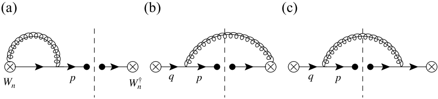
Figure 1: One-loop diagrams for calculation of the heavy quark TMDFF with ${\bf{q}}_{\perp}\sim m$. The vertical dashed lines are the unitary cuts. The self-energy diagrams of the heavy quark are omitted here. Diagrams (a) and (b) have mirror diagrams.

As discussed in Ref. chay:2020jzn , the rapidity divergences originate from the fact that the soft degrees of freedom cannot describe the large rapidity region. Hence, in the calculation of the collinear heavy quark sector, naive collinear contributions do not yield the divergences. Instead, the rapidity divergences occur in the zero-bin contribution Manohar:2006nz , which needs to be subtracted in order to avoid double counting the soft contributions.

The virtual contribution for Fig. 1(a) has been computed in Ref. chay:2020jzn . Including the zero-bin subtraction, the result is

$$M_{a} = \frac{\alpha_{s}C_{F}}{4\pi}\Biggl{[}\frac{2}{\epsilon_{\mathrm{UV}}}+2\ln\frac{\mu^{2}}{m^{2}}+\frac{1}{\epsilon_{\mathrm{IR}}^{2}}+\frac{1}{\epsilon_{\mathrm{IR}}}\ln\frac{\mu^{2}}{m^{2}}+\frac{1}{2}\ln^{2}\frac{\mu^{2}}{m^{2}}+4+\frac{\pi^{2}}{12}$$ (6)

$$~{}~{}~{}~{}~{}~{}~{}~{}+\Bigl{(}\frac{2}{\eta}+2\ln\frac{\nu}{p_{+}}\Bigr{)}\Bigl{(}\frac{1}{\epsilon_{\mathrm{UV}}}-\frac{1}{\epsilon_{\mathrm{IR}}}\Bigr{)}\Biggr{]},$$

where $p_{+}\sim 2E$ is the largest momentum component of the heavy quark in the final state. The rapidity scale that minimizes the large logarithm with $p_{+}$ is $\nu_{c}\sim p_{+}$. Including the mirror contribution of Fig. 1(a) and combining with the self-energy contributions,

$$Z_{\mathcal{Q}}^{(1)}+R_{\mathcal{Q}}^{(1)}=-\frac{\alpha_{s}C_{F}}{4\pi}\Bigl{(}\frac{1}{\epsilon_{\mathrm{UV}}}+\frac{2}{\epsilon_{\mathrm{IR}}}+3\ln\frac{\mu^{2}}{m^{2}}+4\Bigr{)},$$ (7)

the overall virtual contribution is

$$\mathcal{M}_{V}(z,{\bf{q}}_{\perp}) = [2M_{a}+Z_{\mathcal{Q}}^{(1)}+R_{\mathcal{Q}}^{(1)}]\delta(1-z)\delta^{(2)}({\bf{q}}_{\perp})$$ (8)

$$= \frac{\alpha_{s}C_{F}}{2\pi}\Biggl{[}\frac{3}{2\epsilon_{\mathrm{UV}}}+\frac{1}{\epsilon_{\mathrm{IR}}^{2}}+\frac{1}{\epsilon_{\mathrm{IR}}}\Bigl{(}-1+\ln\frac{\mu^{2}}{m^{2}}\Bigr{)}+\frac{1}{2}\ln\frac{\mu^{2}}{m^{2}}++\frac{1}{2}\ln^{2}\frac{\mu^{2}}{m^{2}}+2+\frac{\pi^{2}}{12}$$

$$~{}~{}~{}~{}~{}~{}~{}~{}+\Bigl{(}\frac{2}{\eta}+2\ln\frac{\nu}{p_{+}}\Bigr{)}\Bigl{(}\frac{1}{\epsilon_{\mathrm{UV}}}-\frac{1}{\epsilon_{\mathrm{IR}}}\Bigr{)}\Biggr{]}\delta(1-z)\delta^{(2)}({\bf{q}}_{\perp}).$$

The naive collinear contribution from the real emission in Fig. 1(b) is

$$\tilde{M}_{b}(z,{\bf{q}}_{\perp})=\frac{\alpha_{s}C_{F}}{2\pi^{2}}\frac{\mu^{2}e^{\gamma_{E}}}{\Gamma(1-\epsilon)}\frac{z^{1-2\epsilon}}{1-z}\cdot\frac{({\bf{q}}_{\perp}^{2})^{-\epsilon}}{{\bf{q}}_{\perp}^{2}+\frac{(1-z)^{2}}{z^{2}}m^{2}}\ .$$ (9)

Here, using the plus distribution, we re-express $z/(1-z)$ as

$$\frac{z}{1-z}=\delta(1-z)\Biggl{[}\int^{1}_{0}dx\frac{1-x}{x}\Biggr{]}+\left(\frac{z}{1-z}\right)_{+}.$$ (10)

Then Eq. (9) can be rewritten as

$$\tilde{M}_{b}(z,{\bf{q}}_{\perp}) = \frac{\alpha_{s}C_{F}}{2\pi^{2}}\frac{(\mu^{2}e^{\gamma_{E}})^{\epsilon}}{\Gamma(1-\epsilon)}\Biggl{[}\delta(1-z)\cdot\int^{1}_{0}dx\frac{1-x}{x}\cdot\frac{1}{({\bf{q}}_{\perp}^{2})^{1+\epsilon}}$$

$$\phantom{\frac{\alpha_{s}C_{F}}{2\pi^{2}}\frac{(\mu^{2}e^{\gamma_{E}})^{\epsilon}}{\Gamma(1-\epsilon)}\Biggl{[}}+\left(\frac{z}{1-z}\right)_{+}\cdot\frac{z^{-2\epsilon}({\bf{q}}_{\perp}^{2})^{-\epsilon}}{{\bf{q}}_{\perp}^{2}+\frac{(1-z)^{2}}{z^{2}}2m^{2}}\Biggr{]}\ .$$

To complete calculation, we need to subtract the zero-bin contribution that comes from the underlying soft interaction. Here the soft mode generally scales as

$$p_{s}^{\mu}=(p_{s}^{+},p_{s}^{-},{\bf{p}}^{\perp}_{s})\sim\Bigl{(}\frac{1}{\kappa}q_{\perp},\kappa q_{\perp},q_{\perp}\Bigr{)},~{}~{}q_{\perp}\sim m$$ (12)

where the scaling of the boosting parameter $\kappa$ is given by

$$\frac{m}{Q}\ll\kappa\lesssim 1.$$ (13)

For $\kappa$ is in this range, the soft gluon radiations from the boosted $n$-collinear heavy quark eikonalize satisfying the approximation, $2p_{n}\cdot p_{s}\approx p_{n}^{+}p_{s}^{-}$, giving rise to the soft Wilson line,

$$S_{n}(x)=\mathrm{P}\exp\Bigl{[}ig\int^{\infty}_{x}dsn\cdot A_{s}(sn)\Bigr{]}.$$ (14)

With the scaling behavior of Eq. (12) assigned, the zero-bin contribution for $\tilde{M}_{b}(z,{\bf{q}}_{\perp})$ is given by

$$M_{b}^{\varnothing}(z,{\bf{q}}_{\perp})=\frac{\alpha_{s}C_{F}}{2\pi^{2}}\frac{(\mu^{2}e^{\gamma_{E}})^{\epsilon}}{\Gamma(1-\epsilon)}\left(\frac{\nu}{p_{+}}\right)^{\eta}\left(\int^{\infty}_{0}dxx^{-1-\eta}\right)\frac{1}{({\bf{q}}_{\perp}^{2})^{1+\epsilon}}\cdot\delta(1-z),$$ (15)

where the upper limit of the integral for the gluon momentum fraction $x~{}(=k_{+}/p_{+})$ has been set to infinity since the soft gluon momentum $k_{+}$ in the zero-bin has no upper bound. The rapidity regulator, using Eq. (5), will regulate the rapidity divergence as $k_{+}\to\infty$.

Subtracting Eq. (15) from Eq. (2), the complete contribution for Fig. 1(b) is

$$M_{b}(z,{\bf{q}}_{\perp}) = \tilde{M}_{b}(z,{\bf{q}}_{\perp})-M_{b}^{\varnothing}(z,{\bf{q}}_{\perp})$$

$$= \frac{\alpha_{s}C_{F}}{2\pi^{2}}\frac{(\mu^{2}e^{\gamma_{E}})^{\epsilon}}{\Gamma(1-\epsilon)}\Biggl{[}-\delta(1-z)\Bigl{(}\frac{1}{\eta}+\ln\frac{\nu}{p_{+}}+1\Bigr{)}\frac{1}{({\bf{q}}_{\perp}^{2})^{1+\epsilon}}$$

$$\phantom{\frac{\alpha_{s}C_{F}}{2\pi^{2}}\frac{(\mu^{2}e^{\gamma_{E}})^{\epsilon}}{\Gamma(1-\epsilon)}\Biggl{[}}+\left(\frac{z}{1-z}\right)_{+}\cdot\frac{z^{-2\epsilon}({\bf{q}}_{\perp}^{2})^{-\epsilon}}{{\bf{q}}_{\perp}^{2}+\frac{(1-z)^{2}}{z^{2}}m^{2}}\Biggr{]}.$$

Here the term $1/({\bf{q}}_{\perp}^{2})^{1+\epsilon}$ has a collinear IR divergence when ${\bf{q}}_{\perp}^{2}\to 0$. In order to isolate the divergence we rewrite it as

$$\frac{1}{({\bf{q}}_{\perp}^{2})^{1+\epsilon}} = \delta({\bf{q}}_{\perp}^{2})\Biggl{[}\int^{\Lambda^{2}}_{0}d{\bf{l}}_{\perp}^{2}({\bf{l}}_{\perp}^{2})^{-1-\epsilon}\Biggr{]}+\Biggl{[}\frac{1}{({\bf{q}}_{\perp}^{2})^{1+\epsilon}}\Biggr{]}_{\Lambda^{2}}$$ (17)

$$= \delta({\bf{q}}_{\perp}^{2})\Bigl{(}-\frac{1}{\epsilon_{\mathrm{IR}}}+\ln\Lambda^{2}\Bigr{)}+\Biggl{[}\frac{1}{{\bf{q}}_{\perp}^{2}}\Biggr{]}_{\Lambda^{2}}+\mathcal{O}(\epsilon),$$

where $[\cdots]_{\Lambda^{2}}$ is the so-called $\Lambda^{2}$-distribution, which is the dimensionful plus distribution, defined by

$$[g({\bf{q}}_{\perp}^{2})]_{\Lambda^{2}}=g({\bf{q}}_{\perp}^{2})-\delta({\bf{q}}_{\perp}^{2})\int^{\Lambda^{2}}_{0}d{\bf{l}}_{\perp}^{2}g({\bf{l}}_{\perp}^{2}).$$ (18)

Here $\delta({\bf{q}}_{\perp}^{2})=\pi\delta^{(2)}({\bf{q}}_{\perp})$, and $\Lambda^{2}$ is an arbitrary momentum squared scaling as $\sim{\bf{q}}_{\perp}^{2}$. The overall calculation does not depend on any particular choice of $\Lambda^{2}$ as we will see.

For the second term in the square bracket of Eq. (2), we also employ the $\Lambda^{2}$-distribution by rewriting

$$\frac{(z^{2}{\bf{q}}_{\perp}^{2}/\mu^{2})^{-\epsilon}}{{\bf{q}}_{\perp}^{2}+\frac{(1-z)^{2}}{z^{2}}m^{2}}=f(z,\lambda)\delta({\bf{q}}_{\perp}^{2})+\Biggl{[}\frac{(z^{2}{\bf{q}}_{\perp}^{2}/\mu^{2})^{-\epsilon}}{{\bf{q}}_{\perp}^{2}+\frac{(1-z)^{2}}{z^{2}}m^{2}}\Biggr{]}_{\Lambda^{2}},$$ (19)

where $f(z,\lambda)$ is defined by the following integral

$$f(z,\lambda)=\mu^{2\epsilon}\int^{\Lambda^{2}}_{0}d{\bf{l}}_{\perp}^{2}\frac{(z^{2}{\bf{l}}_{\perp}^{2})^{-\epsilon}}{{\bf{l}}_{\perp}^{2}+\frac{(1-z)^{2}}{z^{2}}m^{2}}=\Bigl{(}\frac{\mu^{2}}{\Lambda^{2}}\Bigr{)}^{\epsilon}\int^{z^{2}}_{0}dy\frac{y^{-\epsilon}}{y+(1-z)^{2}\lambda}~{},$$ (20)

with $\lambda\equiv m^{2}/\Lambda^{2}$. $f(z,\lambda)$ becomes divergent as $z$ goes to 1. Thus, in order to extract the IR divergences fully, we rewrite the combination of $[z/(1-z)]_{+}$ and $f(z,\lambda)$ in Eq. (2) by

$$\left(\frac{z}{1-z}\right)_{+}f(z,\lambda)=\left(\frac{zf(z,\lambda)}{1-z}\right)_{+}+\delta(1-z)\int^{1}_{0}dz^{\prime}\Bigl{(}\frac{z^{\prime}}{1-z^{\prime}}\Bigr{)}\Bigl{[}f(z^{\prime},\lambda)-f(1,\lambda)\Bigr{]}.$$ (21)

Here the first term in the right side is finite $z\to 1$, and the integration in the second term is

$$\frac{e^{\gamma_{E}}}{\Gamma(1-\epsilon)}\int^{1}_{0}dz\Bigl{(}\frac{z}{1-z}\Bigr{)}\Bigl{[}f(z,\lambda)-f(1,\lambda)\Bigr{]}$$

$$~{}~{}~{}=-\frac{1}{2\epsilon_{\mathrm{IR}}^{2}}-\frac{1}{\epsilon_{\mathrm{IR}}}\Bigl{(}1+\frac{1}{2}\ln\frac{\mu^{2}}{m^{2}}\Bigr{)}-\ln\frac{\mu^{2}}{m^{2}}-\frac{1}{4}\ln^{2}\frac{\mu^{2}}{m^{2}}-\frac{\pi^{2}}{24}$$ (22)

$$~{}~{}~{}~{}~{}-\frac{2}{\sqrt{\lambda}}\arctan{\sqrt{\lambda}}-\ln(1+\lambda)-\frac{1}{2}\mathrm{Li}_{2}(-\lambda)-F(\lambda),$$

where $F(\lambda)$ has the following integral form,

$$F(\lambda)=\int^{1}_{0}dz\frac{z}{1-z}\int^{1}_{z^{2}}dy\frac{1}{y+(1-z)^{2}\lambda}\ ,$$ (23)

and $F(\lambda=1)=-\ln 2+\pi^{2}/6$ and $F(0)=-2+\pi^{2}/3$.

Finally, putting Eqs. (17) and (19) into Eq. (2) and using the results in Eqs. (21) and (22), we obtain the real contribution for Fig. 1(b),

$$M_{b}(z,{\bf{q}}_{\perp}) = \frac{\alpha_{s}C_{F}}{2\pi^{2}}\Biggl{\{}\delta(1-z)\Bigl{(}\frac{1}{\eta}+\ln\frac{\nu}{p_{+}}+1\Bigr{)}\Bigl{[}\delta({\bf{q}}_{\perp}^{2})\Bigl{(}\frac{1}{\epsilon_{\mathrm{IR}}}+\ln\frac{\mu^{2}}{\Lambda^{2}}\Bigr{)}-\Bigl{(}\frac{1}{{\bf{q}}_{\perp}^{2}}\Bigr{)}_{\Lambda^{2}}\Bigr{]}$$

$$-\delta(1-z)\delta({\bf{q}}_{\perp}^{2})\Bigl{[}\frac{1}{2\epsilon_{\mathrm{IR}}^{2}}+\frac{1}{\epsilon_{\mathrm{IR}}}\Bigl{(}1+\frac{1}{2}\ln\frac{\mu^{2}}{m^{2}}\Bigr{)}+\ln\frac{\mu^{2}}{m^{2}}+\frac{1}{4}\ln^{2}\frac{\mu^{2}}{m^{2}}+\frac{\pi^{2}}{24}$$

$$+\frac{2}{\sqrt{\lambda}}\arctan{\sqrt{\lambda}}+\ln(1+\lambda)+\frac{1}{2}\mathrm{Li}_{2}(-\lambda)+F(\lambda)\Bigr{]}$$

$$+\delta({\bf{q}}_{\perp}^{2})\Bigl{(}\frac{z}{1-z}\ln\frac{z^{2}+(1-z)^{2}\lambda}{(1-z)^{2}\lambda}\Bigr{)}_{+}+\Bigl{(}\frac{z}{1-z}\Bigr{)}_{+}\Bigl{(}\frac{z^{2}}{z^{2}{\bf{q}}_{\perp}^{2}+(1-z)^{2}m^{2}}\Bigr{)}_{\Lambda^{2}}\Biggr{\}}.$$

We have extracted all the possible IR divergences as ${\bf{q}}_{\perp}^{2}\to 0$ or $z\to 1$ and assigned them to the term with $\delta(1-z)\delta({\bf{q}}_{\perp}^{2})$. The remaining terms with either the plus or the $\Lambda^{2}$-distributions are IR finite.

The contribution for the diagram in Fig. 1(c) is given by

$$M_{c}(z,{\bf{q}}_{\perp}) = \frac{\alpha_{s}C_{F}}{2\pi^{2}}\frac{(\mu^{2}e^{\gamma_{E}})^{\epsilon}}{\Gamma(1-\epsilon)}(1-z)z^{-2\epsilon}({\bf{q}}_{\perp}^{2})^{-\epsilon}$$

$$\times\Biggl{[}\frac{1-\epsilon}{{\bf{q}}_{\perp}^{2}+\frac{(1-z)^{2}}{z^{2}}m^{2}}-\frac{2m^{2}}{z({\bf{q}}_{\perp}^{2}+\frac{(1-z)^{2}}{z^{2}}m^{2})^{2}}\Biggr{]}\equiv M_{c1}(z,{\bf{q}}_{\perp})+M_{c2}(z,{\bf{q}}_{\perp}),$$

where $M_{c1}~{}(M_{c2})$ corresponds to the contribution from the first (second) term in the square bracket. These contributions do not need zero-bin subtractions since the corresponding contribution from the soft mode is power-suppressed.

Due to the presence of $(1-z)$ in the numerator, $M_{c1}$ has no IR divergence. So, ignoring the $\epsilon$ dependence, we obtain

$$M_{c1}(z,{\bf{q}}_{\perp})=\frac{\alpha_{s}C_{F}}{2\pi^{2}}(1-z)\Biggl{[}\ln\frac{z^{2}+(1-z)^{2}\lambda}{(1-z)^{2}\lambda}\cdot\delta({\bf{q}}_{\perp}^{2})+\Bigl{(}\frac{z^{2}}{z^{2}{\bf{q}}_{\perp}^{2}+(1-z)^{2}m^{2}}\Bigr{)}_{\Lambda^{2}}\Biggr{]}.$$ (26)

$M_{c2}$ has an IR divergence as $z\to 1$ and ${\bf{q}}_{\perp}^{2}\to 0$ simultaneously. Using the plus and the $\Lambda^{2}$-distributions we can extract the IR divergence, leading to

$$M_{c2}(z,{\bf{q}}_{\perp}) = \frac{\alpha_{s}C_{F}}{2\pi^{2}}\Biggl{\{}\delta({\bf{q}}_{\perp}^{2})\Biggl{[}\delta(1-z)\Bigl{(}\frac{1}{\epsilon_{\mathrm{IR}}}+\ln\frac{\mu^{2}}{m^{2}}+\frac{2}{\sqrt{\lambda}}\arctan{\sqrt{\lambda}}+\ln(1+\lambda)+G(\lambda)\Bigr{)}$$ (27)

$$-\Bigl{(}\frac{2z^{3}}{(1-z)(z^{2}+(1-z)^{2}\lambda}\Bigr{)}_{+}\Biggr{]}-2z^{3}(1-z)\Bigl{(}\frac{m^{2}}{(z^{2}{\bf{q}}_{\perp}^{2}+(1-z)^{2}m^{2})^{2}}\Bigr{)}_{\Lambda^{2}}\Biggr{\}}.$$

Here $G(\lambda)$ has a form of the integral,

$$G(\lambda)=\int^{1}_{0}dz\int^{1}_{z^{2}}dy\frac{2z(1-z)\lambda}{(y+(1-z)^{2}\lambda)^{2}}\ ,$$ (28)

where $G(0)=0$ and $G(1)=1-\ln 2$.

Finally, combining the results of Eqs. (8), (2), (26), and (27), we obtain the bare one-loop result for the heavy quark TMDFF,

$$D_{\mathcal{Q}/\mathcal{Q}}^{(1)}(z,{\bf{q}}_{\perp}) = \mathcal{M}_{V}(z,{\bf{q}}_{\perp})+2M_{b}(z,{\bf{q}}_{\perp})+M_{c}(z,{\bf{q}}_{\perp})$$

$$= \frac{\alpha_{s}C_{F}}{2\pi^{2}}\Biggl{\{}\delta(1-z)\delta({\bf{q}}_{\perp}^{2})\Biggl{[}\Bigl{(}\frac{2}{\eta}+2\ln\frac{\nu}{p_{+}}+\frac{3}{2}\Bigr{)}\Bigl{(}\frac{1}{\epsilon_{\mathrm{UV}}}+\ln\frac{\mu^{2}}{\Lambda^{2}}\Bigr{)}+2$$

$$-\ln(1+\lambda)-\frac{2}{\sqrt{\lambda}}\arctan{\sqrt{\lambda}}-\mathrm{Li}_{2}(-\lambda)-F(\lambda)+G(\lambda)\Biggr{]}-\delta({\bf{q}}_{\perp}^{2})\Biggl{[}\frac{P_{qq}(z)}{C_{F}}\ln\lambda$$

$$+\left(\frac{2z}{1-z}\Bigl{(}\ln\frac{z^{2}+(1-z)^{2}\lambda}{(1-z)^{2}}-\frac{z^{2}}{z^{2}+(1-z)^{2}\lambda}\Bigr{)}\right)_{+}+(1-z)\ln\frac{z^{2}+(1-z)^{2}\lambda}{(1-z)^{2}}\Biggr{]}$$

$$-\Bigl{(}\frac{2}{\eta}+2\ln\frac{\nu}{p_{+}}+\frac{3}{2}\Bigr{)}\delta(1-z)\left(\frac{1}{{\bf{q}}_{\perp}^{2}}\right)_{\Lambda^{2}}+\frac{P_{qq}(z)}{C_{F}}\left(\frac{z^{2}}{z^{2}{\bf{q}}_{\perp}^{2}+(1-z)^{2}m^{2}}\right)_{\Lambda^{2}}$$

$$-2z^{3}(1-z)\left(\frac{m^{2}}{(z^{2}{\bf{q}}_{\perp}^{2}+(1-z)^{2}m^{2})^{2}}\right)_{\Lambda^{2}}\Biggr{\}}\ .$$

Here $P_{qq}$ is quark-to-quark DokshitzerGribov-Lipatov-Altarelli-Parisi (DGLAP) kernel,

$$P_{qq}(z)=C_{F}\left(\frac{1+z^{2}}{1-z}\right)_{+}.$$ (30)

As shown in Eq. (2), the heavy quark TMDFF is IR finite since the IR divergences from the real emission contributions, $2M_{b}+M_{c}$, are cancelled by the virtual contribution $\mathcal{M}_{V}$. The contributions proportional to $P_{qq}$ involve the logarithm of the heavy quark mass, i.e., $\ln\lambda=\ln m^{2}/\Lambda^{2}$. If we consider the massless limit of the heavy quark, they become collinear-divergent.

Note that UV divergence of the heavy quark TMDFF genuinely comes from the virtual contribution, which makes sense since the real emission contributions with a finite $q_{\perp}$ cannot produce a UV divergence. Even in case with a light quark, we expect the same UV divergence since the inclusion of the quark mass cannot change the UV behavior. The presence of the fermion mass does change the IR behavior and makes it possible to compute the HQ TMDFF perturbatively. Finally, the rapidity divergence for the heavy quark TMDFF is the same as the light-quark case, since the rapidity divergence comes from the zero-bin contributions in the soft sector, which is common for both.

When we consider a generic $N$-jet process, it is useful to introduce multiple rapidity scales $\nu_{i}~{}(i=1,\cdots,N)$ corresponding to the separated $N$ collinear directions chay:2020jzn . In this case, the anomalous dimensions for TMDFFs satisfy the following renormalization group (RG) equations:

$$\frac{d}{d\ln\mu}D_{f/f}(z,{\bf{q}}_{\perp},\mu,\nu_{i}) = \gamma_{f}^{\mu}(\mu,\nu_{i})D_{f/f}(z,{\bf{q}}_{\perp},\mu,\nu_{i}),$$ (31)

$$\frac{d}{d\ln\nu_{i}}D_{f/f}(z,{\bf{q}}_{\perp},\mu,\nu_{i}) = \int d^{2}{\bf{l}}_{\perp}\gamma_{f}^{\nu}({\bf{l}}_{\perp};\mu,\nu_{i})D_{f/f}(z,{\bf{q}}_{\perp}-{\bf{l}}_{\perp},\mu,\nu_{i}),$$

with

$$\gamma_{f}^{\mu}(\mu,\nu_{i}) = \frac{\alpha_{s}}{\pi}\Bigl{(}{\bf{T}}_{f}^{2}\cdot 2\ln\frac{\nu_{i}}{p_{i}^{+}}+\frac{\hat{\gamma}_{f}}{2}\Bigr{)}+\mathcal{O}(\alpha_{s}^{2}),$$ (32)

$$\gamma_{f}^{\nu}({\bf{q}}_{\perp},\mu,\nu_{i}) = \frac{\alpha_{s}}{\pi^{2}}{\bf{T}}_{f}^{2}\Biggl{[}\ln\frac{\mu^{2}}{\Lambda^{2}}\cdot\delta({\bf{q}}_{\perp}^{2})-\Bigl{(}\frac{1}{{\bf{q}}_{\perp}^{2}}\Bigr{)}_{\Lambda^{2}}\Biggr{]}+\mathcal{O}(\alpha_{s}^{2}).$$ (33)

Here ${\bf{T}}_{f}^{2}={\bf{T}}_{f}^{a}\cdot{\bf{T}}_{f}^{a}$ becomes $C_{F}$ for $f=q$ (quark) and $C_{A}$ for $f=g$ (gluon). $\hat{\gamma}_{q}=3C_{F}$ and $\hat{\gamma}_{g}=\beta_{0}$, where $\beta_{0}$ is the leading coefficient of QCD beta function.

In the impact parameter $({\bf{b}})$ space, the heavy quark TMDFF can be expressed through the Fourier transform,

$$\tilde{D}_{H/\mathcal{Q}}(z,{\bf{b}},\mu,\nu)=\int d^{2}{\bf{q}}_{\perp}e^{i{\bf{b}}\cdot{\bf{q}}_{\perp}}D_{H/\mathcal{Q}}(z,{\bf{q}}_{\perp},\mu,\nu).$$ (34)

In ${\bf{b}}$-space, the renormalized result at NLO is

$$\tilde{D}_{\mathcal{Q}/\mathcal{Q}}(z,{\bf{b}},\mu,\nu) = 1+\frac{\alpha_{s}C_{F}}{2\pi}\Biggl{\{}\delta(1-z)\Bigl{[}\Bigl{(}2\ln\frac{\nu}{p_{+}}+\frac{3}{2}\Bigr{)}\ln\bar{b}^{2}\mu^{2}+\frac{1}{2}\ln\bar{b}^{2}m^{2}\Bigr{]}$$

$$+\Bigl{(}\frac{2z}{1-z}\Bigr{)}_{+}\Bigl{[}2K_{0}\Bigl{(}\frac{1-z}{z}mb\Bigr{)}+2\ln(1-z)-1\Bigr{]}$$

$$+2(1-z)K_{0}\Bigl{(}\frac{1-z}{z}mb\Bigr{)}-\Bigl{(}\frac{4z}{1-z}\ln(1-z)\Bigr{)}_{+}$$

$$-2(1-z)\Bigl{[}\frac{bm}{1-z}K_{1}\Bigl{(}\frac{1-z}{z}mb\Bigr{)}-\frac{z}{(1-z)^{2}}\Bigr{]}\Biggr{\}},$$

where $b^{2}={\bf{b}}^{2}$ and $\bar{b}\equiv be^{\gamma_{E}}/2$. $K_{n=0,1}$ are the modified Bessel functions of the second kind. As $z$ goes to 1, the following combinations with the Bessel functions remain nonsingular:

$$K_{0}\Bigl{(}\frac{1-z}{z}mb\Bigr{)}+\ln(1-z) = -\ln m\bar{b}+\mathcal{O}(1-z),$$ (36)

$$\frac{bm}{1-z}K_{1}\Bigl{(}\frac{1-z}{z}mb\Bigr{)}-\frac{z}{(1-z)^{2}} = \frac{m^{2}b^{2}}{4}\Bigl{(}-1+2\ln(1-z)m\bar{b}\Bigr{)}+\mathcal{O}(1-z).$$ (37)

Finally, the leading anomalous dimension for $\tilde{D}_{\mathcal{Q}/\mathcal{Q}}$ satisfying the RG equation, $\frac{d}{d\ln\nu}\tilde{D}_{\mathcal{Q}/\mathcal{Q}}=\gamma_{\mathcal{Q}}^{\nu}\cdot\tilde{D}_{\mathcal{Q}/\mathcal{Q}}$ in ${\bf{b}}$-space is given by

$$\gamma_{\mathcal{Q}}^{\nu}({\bf{b}};\mu,\nu)=\frac{\alpha_{s}C_{F}}{\pi}\ln\bar{b}^{2}\mu^{2}\ .$$ (38)

3 The heavy quark TMD fragmentation function for $q_{\perp}\ll m$

In this section, we consider the region of parameter space where the transverse momentum $q_{\perp}$ is much smaller than the heavy quark mass $m$, so the fluctuations to describe $q_{\perp}$ should be much softer than the collinear interaction scaling shown in Eq. (3). Therefore, the heavy quark can be considered to be boosted, and we can integrate out the collinear interactions. In this boosted heavy quark system, with the collinear interaction being integrated out, the remaining fluctuations are described by the residual interaction, where the momentum scales as

$$k^{\mu}=(k_{+},k_{-},{\bf{k}}_{\perp})\sim\varepsilon Q(1,m^{2}/Q^{2},m/Q).$$ (39)

Here the small parameter $\varepsilon$ has the size $\varepsilon\sim q_{\perp}/m\ll 1$.

This residual interaction can be systematically analyzed in the boosted heavy quark effective theory (bHQET), which can be directly obtained from the massive version of SCET ($\mathrm{SCET_{M}}$) Leibovich:2003jd ; Rothstein:2003wh ; Chay:2005ck . At leading power in the heavy quark limit, the bHQET Lagrangian is given by Kim:2020dgu ; Dai:2021mxb ; Beneke:2023nmj

$$\mathcal{L}^{(0)}_{\mathrm{bHQET}}=\bar{h}_{n}v\cdot iD\frac{{\overline{n}}\!\!\!/}{2}h_{n},$$ (40)

where the boosted heavy quark spinor satisfies the same projection as the spinor in SCET,

$${n}\!\!\!/h_{n}=0,~{}~{}\frac{{n}\!\!\!/{\overline{n}}\!\!\!/}{4}h_{n}=h_{n}.$$ (41)

The velocity in Eq. (40) scales as $v^{\mu}=(v_{+},v_{-},{\bf{v}}_{\perp})\sim(Q/m,m/Q,1)$ and is normalized to $v^{2}=1$.

Therefore, when $q_{\perp}\ll m$, the HQ TMDFF in Eq. (1) can be matched onto bHQET and can be factorized as

$$D_{H/\mathcal{Q}}(z,{\bf{q}}_{\perp}\ll m;\mu,\nu)=C_{\mathcal{Q}}(m,\mu)S_{H/\mathcal{Q}}(z,{\bf{q}}_{\perp},\mu,\nu).$$ (42)

Here $C_{\mathcal{Q}}$ is the matching coefficient onto bHQET obtained from integrating out the virtual collinear interaction, which at NLO is Fleming:2007xt ; Neubert:2007je ; Fickinger:2016rfd

$$C_{\mathcal{Q}}(m,\mu)=1+\frac{\alpha_{s}C_{F}}{4\pi}\Bigl{(}\ln\frac{\mu^{2}}{m^{2}}+\ln^{2}\frac{\mu^{2}}{m^{2}}+4+\frac{\pi^{2}}{6}\Bigr{)}.$$ (43)

$S_{H/\mathcal{Q}}$ is the HQTMD shape function to be described within bHQET, which can be obtained through the direct matching from Eq. (1),

$$S_{H/\mathcal{Q}}(z,{\bf{q}}_{\perp},\mu,\nu) = \sum_{X_{r}}\frac{1}{2N_{c}}\mathrm{Tr}\frac{v_{+}}{2}\langle 0|\delta\bigl{(}\frac{p_{+}}{z}-mv_{+}-i\partial_{+}\bigr{)}\delta^{(2)}({\bf{q}}_{\perp}-{\boldsymbol{\mathcal{P}}}_{\perp})Y_{\overline{n}}^{r\dagger}h_{n}|H(p)X_{r}\rangle$$ (44)

$$~{}~{}~{}\times\langle H(p)X_{r}|\bar{h}_{n}Y_{\overline{n}}^{r}\frac{{\overline{n}}\!\!\!/}{2}|0\rangle,$$

where $X_{r}$ denotes the final states of the residual modes, and $Y_{\overline{n}}^{r}$ is the Wilson line of the residual gluons, which has been matched from $W_{n}$ with collinear gluons integrated out. Here we set the momentum of the final hadron as $p^{\mu}=m_{H}v^{\mu}$ with ${\bf{v}}_{\perp}=0$, where $m_{H}$ is the hadron mass, and the momentum of the initial mother heavy quark is given by $q^{\mu}=mv^{\mu}+k^{\mu}$. Correspondently, the scaling of the transverse momentum is given by ${\bf{q}}_{\perp}={\bf{k}}_{\perp}\sim\varepsilon m\ll m$. $i\partial_{+}$ in the argument of the delta function in Eq. (44) takes the residual momentum of the initial heavy parton, $k_{+}$ and scales as $k_{+}\sim\varepsilon Q\ll Q\sim q_{+}(=mv_{+})$. So the argument of the delta function holds for $z$ is close to 1, and it can be written as

$$\frac{p_{+}}{z}-mv_{+}-k_{+}=\frac{(1-z)mv_{+}}{z}+\frac{\bar{\Lambda}v_{+}}{z}-k_{+}\sim(1-z)mv_{+}+\bar{\Lambda}v_{+}-k_{+},$$ (45)

where $\bar{\Lambda}=m_{H}-m\sim\mathcal{O}(\Lambda_{\mathrm{QCD}})$. Hence this shape function for ${\bf{q}}_{\perp}\ll m$ in Eq. (44) has support in the large $z$ region. At parton level $(H=\mathcal{Q})$, the argument of the delta function in the shape function becomes $(1-z)mv_{+}-i\partial_{+}$, and, at LO in $\alpha_{s}$, the shape function is normalized to

$$S_{\mathcal{Q}/\mathcal{Q}}^{(0)}(z,{\bf{q}}_{\perp})=\delta(1-z)\delta^{(2)}({\bf{q}}_{\perp}).$$ (46)

In obtaining this, we used the following spin sum rule for the boosted heavy quark field Dai:2021mxb ,

$$\sum_{s}h_{n}|\mathcal{Q}_{s}\rangle\langle\mathcal{Q}_{s}|\bar{h}_{n}=m{n}\!\!\!/.$$ (47)

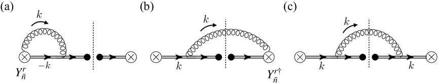
Figure 2: One-loop diagrams for calculating of the heavy quark shape function in bHQET for the $\mathcal{Q}\to\mathcal{Q}$ process. The mirror diagrams for diagrams (a,b) and the self-energy diagram for the heavy quark field are not shown here. The momentum for the final state is $p^{\mu}=mv^{\mu}$ with ${\bf{v}}_{\perp}=0$, while the initial state heavy quark in the real emission diagrams (b, c) has momentum $q^{\mu}=mv^{\mu}+k^{\mu}$ with ${\bf{q}}_{\perp}={\bf{k}}_{\perp}$.

Let us consider the one-loop calculation of the shape function at the parton level. The relevant Feynman diagrams are illustrated in Fig. 2. The virtual contribution corresponding to Fig. 2(a) is chay:2020jzn

$$M_{a}^{r} = \frac{\alpha_{s}C_{F}}{2\pi}\Biggl{[}-\frac{1}{2}\Bigl{(}\frac{1}{\epsilon_{\mathrm{UV}}^{2}}-\frac{1}{\epsilon_{\mathrm{IR}}^{2}}\Bigr{)}-\frac{1}{2}\ln\frac{\mu^{2}}{m^{2}}\Bigl{(}\frac{1}{\epsilon_{\mathrm{UV}}}-\frac{1}{\epsilon_{\mathrm{IR}}}\Bigr{)}$$ (48)

$$\phantom{\frac{\alpha_{s}C_{F}}{2\pi}\Biggl{[}}+\Bigl{(}\frac{1}{\eta}+\ln\frac{\nu}{p_{+}}\Bigr{)}\Bigl{(}\frac{1}{\epsilon_{\mathrm{UV}}}-\frac{1}{\epsilon_{\mathrm{IR}}}\Bigr{)}\Biggr{]}.$$

Like the collinear virtual contribution shown in Eq. (6), the bHQET result has also a rapidity divergence, which comes from the zero-bin contribution to be subtracted in the bHQET calculation. Note that the residual interaction scaling as Eq. (39) has almost the same rapidity as the collinear interaction although the residual mode has smaller energy. Hence, similar to the calculation of the collinear interaction, when we consider the bHQET calculation for the large rapidity region, we need to subtract the contribution of the small rapidity, i.e., the soft contribution. Here the soft interaction is supposed to scale as Eq. (12), but the offshellness is much smaller than $m^{2}$ since $q_{\perp}\ll m$.

For Fig. 2(b), the naive contribution before the zero-bin subtraction is

$$\tilde{M}_{b}^{r}(z,{\bf{q}}_{\perp})=\frac{\alpha_{s}C_{F}}{2\pi^{2}}\frac{\mu^{2}e^{\gamma_{E}}}{\Gamma(1-\epsilon)}\frac{1}{1-z}\cdot\frac{({\bf{q}}_{\perp}^{2})^{-\epsilon}}{{\bf{q}}_{\perp}^{2}+(1-z)^{2}m^{2}}.$$ (49)

When compared with Eq. (9), Eq. (49) can be understood to be in the large $z$ region since the residual gluon emission has small energy, $k_{+}\sim\varepsilon Q$. This means that $(1-z)m$ and ${\bf{q}}_{\perp}$ can be power-counted as the same order, i.e., $(1-z)m\sim q_{\perp}\sim\varepsilon m$. As in Eq. (9), Eq. (49) becomes IR-divergent as $z\to 1$. To isolate the divergence, we employ the plus distribution for $1/(1-z)$,

$$\tilde{M}_{b}^{r}(z,{\bf{q}}_{\perp})=\frac{\alpha_{s}C_{F}}{2\pi^{2}}\frac{(\mu^{2}e^{\gamma_{E}})^{\epsilon}}{\Gamma(1-\epsilon)}\Biggl{[}\delta(1-z)\left(\int^{1}_{0}\frac{dx}{x}\right)\frac{1}{({\bf{q}}_{\perp}^{2})^{1+\epsilon}}+\frac{1}{(1-z)_{+}}\frac{({\bf{q}}_{\perp}^{2})^{-\epsilon}}{{\bf{q}}_{\perp}^{2}+(1-z)^{2}m^{2}}\Biggr{]}.$$ (50)

The zero-bin contribution for Fig. 2(b) is given by

$$M_{b}^{r,\varnothing}(z,{\bf{q}}_{\perp})=\frac{\alpha_{s}C_{F}}{2\pi^{2}}\frac{(\mu^{2}e^{\gamma_{E}})^{\epsilon}}{\Gamma(1-\epsilon)}\left(\frac{\nu}{p_{+}}\right)^{\eta}\int^{\infty}_{0}dxx^{-1-\eta}\frac{1}{({\bf{q}}_{\perp}^{2})^{1+\epsilon}}\cdot\delta(1-z),$$ (51)

where the plus component of the soft gluon momentum is given by $p_{s}^{+}=xp_{+}$ and is assumed to be much smaller than the residual momentum, $k_{+}\sim\varepsilon Q$. Hence this zero-bin contribution only contributes to the part proportional to $\delta(1-z)$. In the integral the momentum fraction $x$ can reach infinity, so this contribution will involve the rapidity divergence.

Subtracting Eq. (51) from Eq. (50), the complete contribution for Fig. 2(b) becomes

$$M_{b}^{r}(z,{\bf{q}}_{\perp}) = \tilde{M}_{b}^{r}-M_{b}^{r,\varnothing}$$ (52)

$$= \frac{\alpha_{s}C_{F}}{2\pi^{2}}\Biggl{\{}\delta(1-z)\Bigl{(}\frac{1}{\eta}+\ln\frac{\nu}{p_{+}}\Bigr{)}\Bigl{[}\delta({\bf{q}}_{\perp}^{2})\Bigl{(}\frac{1}{\epsilon_{\mathrm{IR}}}+\ln\frac{\mu^{2}}{\Lambda^{2}}\Bigr{)}-\Bigl{(}\frac{1}{{\bf{q}}_{\perp}^{2}}\Bigr{)}_{\Lambda^{2}}\Bigr{]}$$

$$\phantom{\frac{\alpha_{s}C_{F}}{2\pi^{2}}\Biggl{\{}}+\frac{(\mu^{2}e^{\gamma_{E}})^{\epsilon}}{\Gamma(1-\epsilon)}\cdot\frac{1}{(1-z)_{+}}\cdot\frac{({\bf{q}}_{\perp}^{2})^{-\epsilon}}{{\bf{q}}_{\perp}^{2}+(1-z)^{2}m^{2}}\Biggr{\}},$$

where we applied Eq. (17), using the $\Lambda^{2}$-distribution to extract IR divergence as ${\bf{q}}_{\perp}^{2}\to 0$. For the second term in the curly bracket, we can also use the $\Lambda^{2}$-distribution in the form

$$\frac{({\bf{q}}_{\perp}^{2}/\mu^{2})^{-\epsilon}}{{\bf{q}}_{\perp}^{2}+(1-z)^{2}m^{2}}=h(z,\lambda)\delta({\bf{q}}_{\perp}^{2})+\Biggl{[}\frac{({\bf{q}}_{\perp}^{2}/\mu^{2})^{-\epsilon}}{{\bf{q}}_{\perp}^{2}+(1-z)^{2}m^{2}}\Biggr{]}_{\Lambda^{2}}.$$ (53)

Here $h(z,\lambda)$ is expressed as the following integral

$$h(z,\lambda)=\mu^{2\epsilon}\int^{\Lambda^{2}}_{0}d{\bf{l}}_{\perp}^{2}\frac{({\bf{l}}_{\perp}^{2})^{-\epsilon}}{{\bf{l}}_{\perp}^{2}+(1-z)^{2}m^{2}}=\Bigl{(}\frac{\mu^{2}}{\Lambda^{2}}\Bigr{)}^{\epsilon}\int^{1}_{0}dy\frac{y^{-\epsilon}}{y+(1-z)^{2}\lambda}~{},$$ (54)

where $\lambda=m^{2}/\Lambda^{2}$. Note that $h(z,\lambda)$ becomes divergent as $z$ goes to 1. Thus, in order to extract the IR divergences, we rewrite the combination of $1/(1-z)_{+}$ and $h(z,\lambda)$ as

$$\frac{1}{(1-z)_{+}}h(z,\lambda)=\left(\frac{h(z,\lambda)}{1-z}\right)_{+}+\delta(1-z)\int^{1}_{0}\frac{dz^{\prime}}{1-z^{\prime}}\Bigl{[}h(z^{\prime},\lambda)-h(1,\lambda)\Bigr{]}.$$ (55)

The integral in the second term produces IR divergences,

$$\frac{e^{\gamma_{E}}}{\Gamma(1-\epsilon)}\int^{1}_{0}\frac{dz}{1-z}\Bigl{[}h(z,\lambda)-h(1,\lambda)\Bigr{]}$$ (56)

$$=-\frac{1}{2\epsilon_{\mathrm{IR}}^{2}}-\frac{1}{2\epsilon_{\mathrm{IR}}}\ln\frac{\mu^{2}}{m^{2}}-\frac{1}{4}\ln^{2}\frac{\mu^{2}}{m^{2}}-\frac{\pi^{2}}{24}-\frac{1}{2}\mathrm{Li}_{2}(-\lambda).$$

Finally, combining the above, $M_{b}^{r}$ can be written as

$$M_{b}^{r}(z,{\bf{q}}_{\perp}) = \frac{\alpha_{s}C_{F}}{2\pi^{2}}\Biggl{\{}\delta(1-z)\Bigl{(}\frac{1}{\eta}+\ln\frac{\nu}{p_{+}}\Bigr{)}\Bigl{[}\delta({\bf{q}}_{\perp}^{2})\Bigl{(}\frac{1}{\epsilon_{\mathrm{IR}}}+\ln\frac{\mu^{2}}{\Lambda^{2}}\Bigr{)}-\Bigl{(}\frac{1}{{\bf{q}}_{\perp}^{2}}\Bigr{)}_{\Lambda^{2}}\Bigr{]}$$

$$-\delta(1-z)\delta({\bf{q}}_{\perp}^{2})\Bigl{[}\frac{1}{2\epsilon_{\mathrm{IR}}^{2}}+\frac{1}{2\epsilon_{\mathrm{IR}}}\ln\frac{\mu^{2}}{m^{2}}+\frac{1}{4}\ln^{2}\frac{\mu^{2}}{m^{2}}+\frac{\pi^{2}}{24}+\frac{1}{2}\mathrm{Li}_{2}(-\lambda)\Bigr{]}$$

$$+\delta({\bf{q}}_{\perp}^{2})\Bigl{(}\frac{1}{1-z}\ln\frac{1+(1-z)^{2}\lambda}{(1-z)^{2}\lambda}\Bigr{)}_{+}+\Bigl{(}\frac{1}{1-z}\Bigr{)}_{+}\Bigl{(}\frac{1}{{\bf{q}}_{\perp}^{2}+(1-z)^{2}m^{2}}\Bigr{)}_{\Lambda^{2}}\Biggr{\}}.$$

The contribution for Fig. 2(c) is given by

$$M_{c}^{r}(z,{\bf{q}}_{\perp})=-\frac{\alpha_{s}C_{F}}{\pi^{2}}\frac{(\mu^{2}e^{\gamma_{E}})^{\epsilon}}{\Gamma(1-\epsilon)}\frac{(1-z)m^{2}({\bf{q}}_{\perp}^{2})^{-\epsilon}}{({\bf{q}}_{\perp}^{2}+(1-z)^{2}m^{2})^{2}}.$$ (58)

The zero-bin contribution to this term is power-suppressed and can be ignored. Eq. (58) becomes IR-divergent when $z\to 1$ and ${\bf{q}}_{\perp}^{2}\to 0$ simultaneously. So employing the plus and $\Lambda^{2}$-distributions we extract IR divergence and obtain

$$M_{c}^{r}(z,{\bf{q}}_{\perp}) = \frac{\alpha_{s}C_{F}}{2\pi^{2}}\Biggl{\{}\delta({\bf{q}}_{\perp}^{2})\Biggl{[}\delta(1-z)\Bigl{(}\frac{1}{\epsilon_{\mathrm{IR}}}+\ln\frac{\mu^{2}}{m^{2}}+\ln(1+\lambda)\Bigr{)}$$

$$~{}~{}~{}~{}~{}~{}~{}-\Bigl{(}\frac{2}{(1-z)(1+(1-z)^{2}\lambda}\Bigr{)}_{+}\Biggr{]}-2(1-z)\Bigl{(}\frac{m^{2}}{({\bf{q}}_{\perp}^{2}+(1-z)^{2}m^{2})^{2}}\Bigr{)}_{\Lambda^{2}}\Biggr{\}}.$$

Finally, together with the self-energy contribution of $h_{n}$,

$$Z_{h}^{(1)}+R_{h}^{(1)}=\frac{\alpha_{s}C_{F}}{2\pi}\Bigl{(}\frac{1}{\epsilon_{\mathrm{UV}}}-\frac{1}{\epsilon_{\mathrm{IR}}}\Bigr{)},$$ (60)

we obtain the complete one loop correction to $S_{\mathcal{Q}/\mathcal{Q}}$,

$$S_{\mathcal{Q}/\mathcal{Q}}^{(1)}(z,{\bf{q}}_{\perp}) = \Bigl{[}2M_{a}^{r}+Z_{h}^{(1)}+R_{h}^{(1)}\Bigr{]}\delta(1-z)\delta({\bf{q}}_{\perp}^{2})+2M_{b}^{r}(z,{\bf{q}}_{\perp})+M_{c}^{r}(z,{\bf{q}}_{\perp})$$

$$= \frac{\alpha_{s}C_{F}}{2\pi^{2}}\Biggl{\{}\delta(1-z)\Bigl{(}\frac{2}{\eta}+2\ln\frac{\nu}{p_{+}}\Bigr{)}\Bigl{[}\delta({\bf{q}}_{\perp}^{2})\Bigl{(}\frac{1}{\epsilon_{\mathrm{UV}}}+\ln\frac{\mu^{2}}{\Lambda^{2}}\Bigr{)}-\Bigl{(}\frac{1}{{\bf{q}}_{\perp}^{2}}\Bigr{)}_{\Lambda^{2}}\Bigr{]}$$

$$+\delta(1-z)\delta({\bf{q}}_{\perp}^{2})\Bigl{[}-\frac{1}{\epsilon_{\mathrm{UV}}^{2}}+\frac{1}{\epsilon_{\mathrm{UV}}}\Bigl{(}1-\ln\frac{\mu^{2}}{m^{2}}\Bigr{)}+\ln\frac{\mu^{2}}{m^{2}}-\frac{1}{2}\ln^{2}\frac{\mu^{2}}{m^{2}}-\frac{\pi^{2}}{12}$$

$$+\ln(1+\lambda)-\mathrm{Li}_{2}(-\lambda)\Bigr{]}+\delta({\bf{q}}_{\perp}^{2})\Bigl{[}\frac{2}{1-z}\Bigl{(}\ln\frac{1+(1-z)^{2}\lambda}{(1-z)^{2}\lambda}-\frac{1}{1+(1-z)^{2}\lambda}\Bigr{)}\Bigr{]}_{+}$$

$$+\frac{2}{(1-z)_{+}}\Bigl{(}\frac{1}{{\bf{q}}_{\perp}^{2}+(1-z)^{2}m^{2}}\Bigr{)}_{\Lambda^{2}}-2(1-z)\Bigl{(}\frac{m^{2}}{({\bf{q}}_{\perp}^{2}+(1-z)^{2}m^{2})^{2}}\Bigr{)}_{\Lambda^{2}}\Biggr{\}}.$$

Here, as we expect, we see that IR divergences exactly cancel. The remaining UV divergences arise entirely from the virtual contributions ($2M_{a}^{r}+Z_{h}^{(1)}$). Also note the rapidity divergence is the same as the one for the TMDFF with ${\bf{q}}_{\perp}\sim m$ as shown in Eq. (2).

In ${\bf{b}}$-space, the renormalized HQTMD shape function at NLO is given by

$$\tilde{S}_{\mathcal{Q}/\mathcal{Q}}(z,{\bf{b}};\mu,\nu) = \int d^{2}{\bf{q}}_{\perp}e^{i{\bf{b}}\cdot{\bf{q}}_{\perp}}S_{\mathcal{Q}}(z,{\bf{q}}_{\perp};\mu,\nu)$$ (62)

$$= \delta(1-z)+\frac{\alpha_{s}C_{F}}{2\pi}\Biggl{\{}\delta(1-z)\Bigl{(}2\ln\frac{\nu}{p_{+}}\ln\bar{b}^{2}\mu^{2}+\ln\frac{\mu^{2}}{m^{2}}-\frac{1}{2}\ln^{2}\frac{\mu^{2}}{m^{2}}-\frac{\pi^{2}}{12}\Bigr{)}$$

$$-\Bigl{[}\frac{2}{1-z}(1+2\ln(1-z))\Bigr{]}_{+}+\frac{4}{(1-z)_{+}}\Bigl{[}K_{0}((1-z)mb)+\ln(1-z)\Bigr{]}$$

$$-2(1-z)\Bigl{[}\frac{bm}{1-z}K_{1}((1-z)mb)-\frac{1}{(1-z)^{2}}\Bigr{]}\Biggr{\}}.$$

Here $b$ is power-counted as $b\sim 1/q_{\perp}\sim 1/(\varepsilon m)$, hence the combination $(1-z)mb$ is of $\mathcal{O}(1)$. The leading anomalous dimensions from the RG equations,

$$\frac{d}{d\ln s}\tilde{S}_{\mathcal{Q}}(z,{\bf{b}};s)=\gamma^{s}_{r}\cdot\tilde{S}_{\mathcal{Q}}(z,{\bf{b}};s),~{}~{}s=\mu,\nu,$$ (63)

are given by

$$\gamma_{r}^{\mu}(\mu,\nu) =\frac{\alpha_{s}C_{F}}{\pi}\Bigl{(}2\ln\frac{m\nu}{p_{+}\mu}+1\Bigr{)},$$ (64)

$$\gamma_{r}^{\nu}({\bf{b}};\mu,\nu) =\frac{\alpha_{s}C_{F}}{\pi}\ln\bar{b}^{2}\mu^{2}.$$ (65)

From Eqs. (64) and (65), we can extract the characteristic scales to minimize the large logarithms for the resummation of $\tilde{S}_{\mathcal{Q}/\mathcal{Q}}$,

$$\mu_{r}\sim\frac{1}{\bar{b}},~{}~{}\nu_{r}\sim\frac{p_{+}}{m\mu_{r}}\sim\frac{p_{+}\bar{b}}{m}.$$ (66)

Thus we see that $\nu_{r}$ has the same scaling as the large component of the residual momentum shown in Eq. (39).

As a consistency check between the $\mathrm{SCET_{M}}$ and bHQET calculations, we take the limit of $\tilde{D}_{\mathcal{Q}/\mathcal{Q}}(z,{\bf{b}})$ in Eq. (2) as $z$ goes to 1 with power counting $mb\sim(1-z)^{-1}$. This result coincides with the combination of $C_{\mathcal{Q}}$ and $S_{\mathcal{Q}/\mathcal{Q}}$ at NLO found above:

$$\tilde{D}_{\mathcal{Q}/\mathcal{Q}}^{(1)}(z\to 1,{\bf{b}}\sim m^{-1}(1-z)^{-1},\mu,\nu)=C_{\mathcal{Q}}^{(1)}(m,\mu)+\tilde{S}_{\mathcal{Q}/\mathcal{Q}}^{(1)}(z,{\bf{b}},\mu,\nu)$$

$$~{}~{}=\frac{\alpha_{s}C_{F}}{2\pi}\Biggl{\{}\delta(1-z)\Bigl{[}2\ln\frac{\nu}{p_{+}}\cdot\ln\bar{b}^{2}\mu^{2}+\frac{3}{2}\ln\frac{\mu^{2}}{m^{2}}+2\Bigr{]}-\Bigl{[}\frac{2}{1-z}(1+2\ln(1-z))\Bigr{]}_{+}$$ (67)

$$~{}~{}+\frac{4}{(1-z)_{+}}\Bigl{[}K_{0}((1-z)mb)+\ln(1-z)\Bigr{]}-2(1-z)\Bigl{[}\frac{bm}{1-z}K_{1}((1-z)mb)-\frac{1}{(1-z)^{2}}\Bigr{]}\Biggr{\}}\ .$$

4 Full description on the heavy quark TMD fragmentation function

4.1 The TMD fragmentation function when ${\bf{q}}_{\perp}\gg m$

When $q_{\perp}\gg m$, the HQ TMDFF in Eq. (1) can be factorized due to this hierarchy of scales. To accomplish this, we need to first integrate out the fluctuations of ${\bf{q}}_{\perp}^{2}$, then consider the fragmentation to the hadron at the lower scale $\mu\sim m$. Thus, the HQ TMDFF in this case can be matched onto the standard heavy quark fragmentation function (HQ FF), which only depends on the longitudinal momentum fraction of the hadron. In ${\bf{b}}$-space, the factorization reads

$$\tilde{D}_{H/\mathcal{Q}}(z,{\bf{b}};\mu,\nu)=\sum_{k}\int^{1}_{z}\frac{dx}{x}K_{k/\mathcal{Q}}(x,{\bf{b}};\mu,\nu)D_{H/k}\bigl{(}\frac{z}{x},\mu\bigr{)}+\mathcal{O}(mb),$$ (68)

where $D_{H/k}(z/x)$ is the standard FF to the heavy hadron $H$, and $k$ is the flavor of the fragmenting parton. Except for the case $k=\mathcal{Q}$, the contributions from other partons are suppressed by at least $\alpha_{s}^{2}$ and can be ignored to the order we are considering. Note that since we are considering the limit $q_{\perp}\gg m$, here $mb\ll 1$.

From the NLO result of $\tilde{D}_{\mathcal{Q}/\mathcal{Q}}(z,{\bf{b}})$ in Eq. (2), we can directly obtain the NLO result of $K_{\mathcal{Q}/\mathcal{Q}}$ in Eq. (68) by matching onto the FF, $D_{\mathcal{Q}/\mathcal{Q}}(z/x)$. The result of Eq. (2) was been obtained with treatment of $mb\sim\mathcal{O}(1)$, hence it can be considered as the full result in an expansion of $mb$. We must, therefore, extract the leading result from Eq. (2) in the limit $mb\to 0$. Accordingly, the following combinations of the Bessel functions in Eq. (2) can be expanded as

$$K_{0}\Bigl{(}\frac{1-z}{z}mb\Bigr{)}+\ln(1-z) =-\ln m\bar{b}+\ln z+\mathcal{O}(mb),$$ (69)

$$\frac{bm}{1-z}K_{1}\Bigl{(}\frac{1-z}{z}mb\Bigr{)}-\frac{z}{(1-z)^{2}} =\frac{m^{2}b^{2}}{4z}\Bigl{(}-1+2\ln(1-z)m\bar{b}\Bigr{)}+\mathcal{O}(m^{3}b^{3}).$$ (70)

The combination with $K_{1}$ can be safely ignored in this limit, and using Eq. (69) we obtain

$$\tilde{D}_{\mathcal{Q}/\mathcal{Q}}\bigl{(}z,{\bf{b}}\ll\frac{1}{m};\mu,\nu\bigr{)} =1+\frac{\alpha_{s}C_{F}}{2\pi}\Biggl{\{}\delta(1-z)\cdot\Bigl{(}2\ln\frac{\nu}{p_{+}}+\frac{3}{2}\Bigr{)}\ln\bar{b}^{2}\mu^{2}$$ (71)

$$-\Bigl{[}\frac{1+z^{2}}{1-z}\bigl{(}\ln m^{2}\bar{b}^{2}(1-z)^{2}+1\bigr{)}\Bigr{]}_{+}+\Bigl{(}\frac{4z}{1-z}\Bigr{)}_{+}\ln z+(1-z)(1+2\ln z)\Biggr{\}}\ .$$

The NLO result for the standard HQ FF is well known, Mele:1990cw

$$D_{\mathcal{Q}/\mathcal{Q}}(z,\mu)=\delta(1-z)+\frac{\alpha_{s}C_{F}}{2\pi}\Bigl{[}\frac{1+z^{2}}{1-z}\Bigl{(}\ln\frac{\mu^{2}}{m^{2}(1-z)}-1\Bigr{)}\Bigr{]}.$$ (72)

By subtracting this from the one-loop result of Eq. (71) we obtain the one-loop result of $K_{\mathcal{Q}/\mathcal{Q}}$,

$$K_{\mathcal{Q}/\mathcal{Q}}^{(1)}(z,{\bf{b}};\mu,\nu) =\tilde{D}^{(1)}_{\mathcal{Q}/\mathcal{Q}}\bigl{(}z,{\bf{b}}\ll\frac{1}{m};\mu,\nu\bigr{)}-D_{\mathcal{Q}/\mathcal{Q}}^{(1)}(z,\mu)$$ (73)

$$=\frac{\alpha_{s}C_{F}}{2\pi}\Bigl{[}\delta(1-z)\Bigl{(}2\ln\frac{\nu}{p_{+}}+\frac{3}{2}\Bigr{)}\ln\bar{b}^{2}\mu^{2}-\Bigl{(}\frac{1+z^{2}}{1-z}\Bigr{)}_{+}\ln\frac{\bar{b}^{2}}{z^{2}}\mu^{2}+1-z\Bigr{]}\ .$$

As expected, the TMD kernel $K_{\mathcal{Q}/\mathcal{Q}}$ does not depend on the heavy quark mass $m$ and its characteristic scale is of order $\mu\sim 1/\bar{b}$.

4.2 Nonperturbative contribution to the fragmentation function when ${\bf{q}}_{\perp}\gg\Lambda_{\rm QCD}$

Thus far we have not considered the hadronization effects governed by nonperturbative physics at scale $\Lambda_{\mathrm{QCD}}$. For a heavy-light hadron $H$ involving a heavy quark, like a $B$ meson, the hadronization in the fragmenting process is through low energy interactions of the heavy quark, adequately described by bHQET. Further, in bHQET the interactions are entirely mediated by the residual gluon that carries only small fraction of the energy. Hence the fragmenting process for hadronization dominantly occurs in the large-$z$ region where the heavy quark in the final state carries most of the energy in the process.

To include the nonperturbative contribution, the standard HQ FF can be written as Nason:1999zj ; Cacciari:2005uk ; Fickinger:2016rfd

$$D_{H/i}(x,\mu)=\int^{1}_{x}\frac{dz}{z}D_{\mathcal{Q}/i}\Bigl{(}\frac{x}{z},\mu\Bigr{)}\phi_{H/\mathcal{Q}}(z),$$ (74)

where $D_{Q/i}$ is the FF at the parton level to be computed perturbatively and $\phi_{H/\mathcal{Q}}$ is the nonpertubative piece describing the modification due to hadronization. The distribution $\phi_{H/\mathcal{Q}}$ is strongly peaked in the large-$z$ region. When the $x$ in $D_{H/i}(x)$ probes the region far away from the endpoint, i.e., $1-x\sim\mathcal{O}(1)$, $\phi_{H/\mathcal{Q}}$ acts like a delta function,

$$\phi_{H/\mathcal{Q}}(z)\approx N_{H}\delta(1-z),$$ (75)

where $N_{H}$ is the nonperturbative fractional parameter for the hadronization. In bHQET, $N_{H}$ is defined by Fickinger:2016rfd

$$N_{H}=\frac{1}{4N_{c}m_{H}}\sum_{X_{r}}\mathrm{Tr}\langle 0|Y_{\overline{n}}^{r\dagger}h_{n}|H_{v}X_{r}\rangle\langle H_{v}X_{r}|\bar{h}_{n}Y_{\overline{n}}^{r}\frac{{\overline{n}}\!\!\!/}{2}|0\rangle,$$ (76)

where $|H_{v}\rangle=|H\rangle/\sqrt{m_{H}}$. When we consider the sum over all the hadrons containing the heavy quark, it should satisfy $\sum_{H}N_{H}=1$.

In Eq. (74), the NLO perturbative result for $D_{\mathcal{Q}/\mathcal{Q}}$ was shown in Eq. (72), while the result for $D_{\mathcal{Q}/g}$ reads Mele:1990cw

$$D_{\mathcal{Q}/g}(z,\mu) =\frac{\alpha_{s}}{2\pi}\frac{z^{2}+(1-z)^{2}}{2}\ln\frac{\mu^{2}}{m^{2}}\ .$$ (77)

As $z$ is approaches 1, $D_{\mathcal{Q}/\mathcal{Q}}$ dominates over $D_{\mathcal{Q}/g}$ and, similarly to Eq. (42), it factorizes

$$D_{\mathcal{Q}/\mathcal{Q}}(z\to 1,\mu)=C_{\mathcal{Q}}(m,\mu)S_{\mathcal{Q}/\mathcal{Q}}(z,\mu),$$ (78)

where $C_{\mathcal{Q}}$ was introduced in Eq. (43), and $S_{\mathcal{Q}/\mathcal{Q}}(z)$ at NLO is given by Neubert:2007je ; Fickinger:2016rfd

$$S_{\mathcal{Q}/\mathcal{Q}}(z,\mu)=\delta(1-z)+\frac{\alpha_{s}C_{F}}{2\pi}\Biggl{\{} \delta(1-z)\Bigl{(}\ln\frac{\mu^{2}}{m^{2}}-\frac{1}{2}\ln^{2}\frac{\mu^{2}}{m^{2}}-\frac{\pi^{2}}{12}\Bigr{)}$$ (79)

$$+\Bigl{[}\frac{2}{1-z}\Bigl{(}\ln\frac{\mu^{2}}{m^{2}(1-z)^{2}}-1\Bigr{)}\Bigr{]}_{+}\Biggr{\}}\ .$$

When we consider nonperturbative implications for the HQ TMDFF with ${\bf{q}}_{\perp}\gg\Lambda_{\mathrm{QCD}}$, we can basically apply the same approach as Eq. (74), hence we will employ the same nonperturbative function. As a result, when ${\bf{q}}_{\perp}\gg\Lambda_{\mathrm{QCD}}$, the HQ TMDFF can be written as

$$D_{H/i}(x,{\bf{q}}_{\perp},\mu,\nu)=\int^{1}_{x}\frac{dz}{z}D_{\mathcal{Q}/i}(z,{\bf{q}}_{\perp},\mu,\nu)\phi_{H/\mathcal{Q}}(z).$$ (80)

Here the NLO result of $D_{\mathcal{Q}/i=\mathcal{Q}}$ was obtained in Eq. (2), and the one loop result of $D_{\mathcal{Q}/g}$ is

$$D_{\mathcal{Q}/g}(z,{\bf{q}}_{\perp},\mu)=\frac{\alpha_{s}T_{F}}{2\pi}\frac{1}{{\bf{q}}_{\perp}^{2}+m^{2}/z^{2}}\Bigl{[}1-2z(1-z)\frac{{\bf{q}}_{\perp}^{2}}{{\bf{q}}_{\perp}^{2}+m^{2}/z^{2}}\Bigr{]},$$ (81)

where $T_{F}=1/2$.

When ${\bf{q}}_{\perp}$ is much smaller than the heavy quark mass $m$, $D_{\mathcal{Q}/\mathcal{Q}}$ dominates over $D_{\mathcal{Q}/g}$ and, as shown in Eq. (42), $D_{\mathcal{Q}/\mathcal{Q}}$ can be additionally factorized as

$$D_{\mathcal{Q}/\mathcal{Q}}(z,{\bf{q}}_{\perp}\ll m,\mu,\nu)=C_{\mathcal{Q}}(m,\mu)S_{\mathcal{Q}/\mathcal{Q}}(z,{\bf{q}}_{\perp},\mu,\nu).$$ (83)

We have also discussed the HQ TMDFF for ${\bf{q}}_{\perp}\gg m$ in subsection 4.1. As shown there, the TMDFF can be matched onto the standard FF with the fluctuations of ${\bf{q}}_{\perp}^{2}$ integrated out. Therefore, the nonperturbative piece can be genuinely included in the standard FF as in Eq. (74).

For the parameterization of the nonperturbative FF, $\phi_{H/\mathcal{Q}}$, we adopt the model introduced in Ref. Neubert:2007je ; Fickinger:2016rfd ,

$$\phi_{H/\mathcal{Q}}(z)=N_{H}\frac{m}{\lambda_{H}}\frac{(p+1)^{p+1}}{\Gamma(p+1)}\Bigl{(}\frac{m}{\lambda_{H}}(1-z)\Bigr{)}^{p}e^{-(p+1)(1-z)m/\lambda_{H}}.$$ (84)

This was originally introduced in momentum space in $\hat{\omega}=(1-z)mv_{+}$, where $\phi_{H/Q}(\hat{\omega})=\phi_{H/\mathcal{Q}}(z)\cdot|dz/d\hat{\omega}|$. The integral over the full range of $\hat{\omega}$ is normalized to unity,

$$\int^{\infty}_{0}d\hat{\omega}~{}\phi_{H/Q}(\hat{\omega})=1.$$ (85)

$\lambda_{H}$ in Eq. (84) is a quantity of order $\Lambda_{\rm QCD}$ and is related to the first moment of $\phi_{H/Q}(\hat{\omega})$,

$$\int^{\infty}_{0}d\hat{\omega}~{}\hat{\omega}\phi_{H/Q}(\hat{\omega})=\frac{\lambda_{H}}{v_{+}}\ .$$ (86)

One advantage of using Eq. (84) is that, in the limit $m/\lambda_{H}\to\infty$, the nonperturbative FF becomes $\phi_{H/\mathcal{Q}}\approx N_{H}\delta(1-z)$. So, as long as $m/\lambda_{H}$ is a large value much greater than 1, the nonperturbative effects predominantly make an impact on the endpoint region with $1-z\sim\mathcal{O}(\Lambda/m)$. Away from the endpoint, the nonperturbative effects are small.

4.3 Summary: the HQ TMDFF with ${\bf{q}}_{\perp}\gg\Lambda_{\rm{QCD}}$

In this subsection, we summarize our results of the HQ TMDFF with the different hierarchies between ${\bf{q}}_{\perp}$ and $m$. With the assumption that ${\bf{q}}_{\perp}\gg\Lambda_{\rm{QCD}}$, we can describe the transverse-momentum dependent part purturbatively and can put the nonperturbative effects fully into $\phi_{H/\mathcal{Q}}$. Here we show the TMDFFs in the ${\bf{b}}$-space comparing the sizes of $b$ and $1/m$:

1. $b\ll 1/m~{}(q_{\perp}\gg m)$

   $$\tilde{D}_{H/i}(z,{\bf{b}},\mu,\nu)=\sum_{j}\int^{1}_{z}\frac{dx}{x}K_{j/i}(x,{\bf{b}},\mu,\nu)D_{H/j}\bigl{(}\frac{z}{x},\mu\bigr{)}+\mathcal{O}(mb),$$ (87)

   where, from Eq. (74),

   $$D_{H/j}\bigl{(}\frac{z}{x},\mu)=\int^{1}_{z/x}\frac{dy}{y}D_{\mathcal{Q}/j}(y,\mu)\phi_{H/\mathcal{Q}}\bigl{(}\frac{z}{xy}\bigr{)}.$$ (88)

   Here the one loop result of the TMD kernel $K_{\mathcal{Q}/\mathcal{Q}}$ was presented in Eq. (73). We also computed the one-loop results for the kernels with other flavors, which are

   $$K^{(1)}_{g/q}(z,{\bf{b}},\mu) =\frac{\alpha_{s}C_{F}}{2\pi}\Bigl{[}-\frac{1+(1-z)^{2}}{z}\ln\frac{\bar{b}^{2}\mu^{2}}{z^{2}}+z\Bigr{]}\ ,$$ (89)

   $$K^{(1)}_{q/g}(z,{\bf{b}},\mu) =\frac{\alpha_{s}T_{F}}{2\pi}\Bigl{[}-\bigl{(}z^{2}+(1-z)^{2})\ln\frac{\bar{b}^{2}\mu^{2}}{z^{2}}-2z(1-z)\Bigr{]}\ ,$$ (90)

   $$K^{(1)}_{g/g}(z,{\bf{b}},\mu,\nu) =\frac{\alpha_{s}C_{A}}{2\pi}\Bigl{\{}\delta(1-z)\cdot 2\ln\frac{\nu}{p_{+}}\ln\bar{b}^{2}\mu^{2}$$ (91)

   $$~{}~{}~{}-2\Bigl{[}\frac{z}{(1-z)_{+}}+\frac{1-z}{z}+z(1-z)\Bigr{]}\ln\frac{\bar{b}^{2}\mu^{2}}{z^{2}}\Bigr{\}}\ .$$

2. $b\sim 1/m~{}(q_{\perp}\sim m)$

   $$\tilde{D}_{H/i}(z,{\bf{b}},\mu,\nu)=\int^{1}_{z}\frac{dx}{x}\tilde{D}_{\mathcal{Q}/i}(x,{\bf{b}},\mu,\nu)\phi_{H/\mathcal{Q}}\bigl{(}\frac{z}{x}\bigr{)}.$$ (92)

   Here the NLO result of $\tilde{D}_{\mathcal{Q}/\mathcal{Q}}(z,{\bf{b}})$ was obtained in Eq. (2), and the Fourier transform of Eq. (81), $\tilde{D}_{\mathcal{Q}/g}$, is given by

   $$\tilde{D}_{\mathcal{Q}/g}(z,{\bf{b}},\mu)=\frac{\alpha_{s}T_{F}}{\pi}\Bigl{[}(z^{2}+(1-z)^{2})K_{0}\bigl{(}\frac{mb}{z}\bigr{)}-(1-z)mbK_{1}\bigl{(}\frac{mb}{z}\bigr{)}\Bigr{]}\ .$$ (93)

3. $1/\Lambda_{\rm QCD}\gg b\gg 1/m~{}(m\gg q_{\perp}\gg\Lambda_{\rm QCD})$

   In this case, $\tilde{D}_{H/i}(z,{\bf{b}})$ is approximated by $\tilde{D}_{H/\mathcal{Q}}(z,{\bf{b}})$, and $\tilde{D}_{\mathcal{Q}/\mathcal{Q}}(z,{\bf{b}})$ can be refactorized to $C_{\mathcal{Q}}(m)\cdot\tilde{S}_{\mathcal{Q}/\mathcal{Q}}(z,{\bf{b}})$, which is the Fourier transform of Eq. (83). Therefore,

   $$\tilde{D}_{H/i}(z,{\bf{b}},\mu,\nu)=C_{\mathcal{Q}}(m,\mu)\int^{1}_{z}\frac{dx}{x}\tilde{S}_{\mathcal{Q}/\mathcal{Q}}(x,{\bf{b}},\mu,\nu)\phi_{H/\mathcal{Q}}\bigl{(}\frac{z}{x}\bigr{)}+\mathcal{O}\bigl{(}\frac{1}{mb}\bigr{)},$$ (94)

   where the NLO results of $C_{\mathcal{Q}}$ and $\tilde{S}_{\mathcal{Q}/\mathcal{Q}}$ were presented in Eqs. (43) and (62), respectively.

5 The heavy quark TMD jet fragmentation function

In this section, as an application of the HQ TMDFF, we will analyze heavy quark fragmentation inside a given observed jet constructing the factorization theorem for the HQ TMD jet fragmentation function (JFF). By considering the TMD fragmenting process within a jet, we can closely delineate the substructure of a jet involving the heavy quark and acquire direct or useful information on the hadronization of the heavy quark.

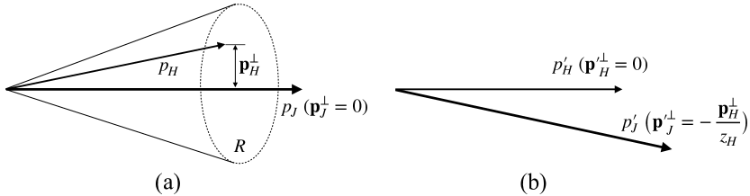
Figure 3: (a): Description of fragmentation to the hadron inside a jet with radius $R$ in the jet frame, where the transverse momentum of the jet is set to zero. (b): Description of the fragmentation in the hadron frame. Here the momentum fraction, $z_{H}=p_{H}^{+}/p_{J}^{+}$, is the same in both frames.

As illustrated in Fig. 3(a), we consider the transverse momentum distribution of the hadron with respect to the standard jet axis, which lies along the total momentum of the jet. For a jet with small radius $R$, the typical jet size is $E_{J}R$ for $e^{+}e^{-}$ annihilation or $p_{J}^{T}R$ for hadronic collisions, where $p_{J}^{T}$ is the large transverse momentum relative to the beam axis. Since we are considering the small transverse momentum distribution of the hadron relative to the jet axis, ${\bf{p}}^{\perp}_{H}$, we will assign the limit ${\bf{p}}^{\perp}_{H}\ll E_{J}R,~{}p_{J}^{T}R$. Then the transverse motion of the hadron is described by collinear and collinear-soft (csoft) interactions, whose momenta scale as

$$p_{c}^{\mu} = (p_{c}^{+},p_{c}^{-},{\bf{p}}^{\perp}_{c})\sim(E_{J},p_{H}^{\perp 2}/E_{J},p_{H}^{\perp}),$$ (95)

$$p_{cs}^{\mu} = (p_{cs}^{+},p_{cs}^{-},{\bf{p}}^{\perp}_{cs})\sim(p_{H}^{\perp}/R,p_{H}^{\perp}R,p_{H}^{\perp}),$$ (96)

where $p_{H}^{\perp}\equiv|{\bf{p}}^{\perp}_{H}|$. Note that csoft interactions can discern the jet boundary, while collinear interactions cannot.

In building up the factorization theorem, as illustrated in Fig 3(b), it is convenient to consider this fragmentation process in the hadron frame because the factorization usually describes TMD behaviors of the (collinear/csoft) overall initiating partons. In the hadron frame the total transverse momentum inside the jet is nonzero, and is related to the transverse momentum of the hadron in the jet frame that is an observable in the experiment by

$${\bf{q}}_{\perp}\equiv{\bf{p^{\prime}}}^{\perp}_{J}=\sum_{i\in J}{\bf{p^{\prime}}}^{\perp}_{c,i}+\sum_{j\in J}{\bf{p^{\prime}}}^{\perp}_{cs,j}=-\frac{{\bf{p}}^{\perp}_{H}}{z_{H}}.$$ (97)

Here ${\bf{p}}^{\perp}_{H}$ is the momentum in the jet frame and we denoted the momenta in the hadron frame with primes.

5.1 The TMD JFF module

Focusing on the inclusive jet production, for $e^{+}e^{-}$ annihilation the (inclusive) TMD JFF can be defined as

$$F_{J}(z_{H},{\bf{p}}^{\perp}_{H};E_{J},R)=\frac{d\sigma(e^{+}e^{-}\to J(H)X)}{dE_{J}dz_{H}d^{2}{\bf{p}}^{\perp}_{H}}\Biggl{/}\frac{d\sigma(e^{+}e^{-}\to JX)}{dE_{J}}\ ,$$ (98)

where $J(H)$ denotes the jet that includes the hadron $H$. In hadron collisions, we can similarly define the JFF considering the differential cross section on $p_{T}^{J}$ (as well as rapidity) rather than $E_{J}$. For clustering a jet, we consider the anti-$\mathrm{k_{T}}$ algorithm Cacciari:2008gp ; Ellis:2010rwa . If the jet radius $R$ is small, the cross sections in Eq. (98) are factorized into the hard and jet parts. For the jet containing $H$ we have

$$\frac{d\sigma(e^{+}e^{-}\to J(H)X)}{dE_{J}dz_{H}d^{2}{\bf{p}}^{\perp}_{H}} = \frac{d\sigma(e^{+}e^{-}\to J(H)X)}{z_{H}^{2}dE_{J}dz_{H}d^{2}{\bf{q}}_{\perp}}$$ (99)

$$= \sum_{k}\int^{1}_{x_{J}}\frac{dx}{x}\frac{d\hat{\sigma}}{dE_{k}}\left(\frac{x_{J}}{x},\mu\right)\cdot\frac{1}{z_{H}^{2}}\mathcal{G}_{J(H)/k}(x,z_{H},{\bf{q}}_{\perp},E_{J},R,\mu)$$

where $\hat{\sigma}$ is the partonic cross section and $\mathcal{G}_{J(H)/k}$ is the semi-inclusive TMD fragmenting jet function from parton $k$ to hadron $H$ inside the jet $J$. This formalism has been applied to jet production with massless partons Kang:2017glf . As denoted in Eq. (97), ${\bf{q}}_{\perp}$ is the jet transverse momentum in the hadron frame and the longitudinal momentum variables in Eq. (99) are

$$x_{J}=\frac{2p_{\rm tot}\cdot p_{J}}{p_{\rm tot}^{2}}=\frac{2E_{J}}{Q}\sim\frac{p_{J}^{+}}{Q},~{}~{}x=\frac{p_{J}^{+}}{p_{k}^{+}},~{}~{}z_{H}=\frac{p_{H}^{+}}{p_{J}^{+}}\ ,$$ (100)

where $p_{\rm tot}$ is the total momentum of the incoming electron and positron, and $p_{\rm tot}^{2}=Q^{2}$. Here the parton $k$, the jet $J$, and the hadron $H$ are all described to be collinear in the $n$-direction.

Since we are taking the limit $E_{J}R\gg{\bf{q}}_{\perp}$, the jet function $\mathcal{G}_{J(H)/k}$ can be further factorized. In this case it is useful to express the factorization using the fragmentation function to a jet (FFJ) Kang:2016mcy ; Dai:2016hzf . To NLO in $\alpha_{s}$, we can refactorize $\mathcal{G}_{J(H)/k}$ as Dai:2016hzf ; Dai:2018ywt

$$\mathcal{G}_{J(H)/k}(x,z_{H},{\bf{q}}_{\perp},E_{J},R,\mu)=\sum_{l}D_{J_{l}/k}(x,E_{J}R,\mu)\Phi_{H/J_{l}}(z_{H},{\bf{q}}_{\perp};E_{J},R).$$ (101)

Here $D_{J_{l}/k}$ is the FFJ from parton $k$ to $J_{l}$, where $J_{l}$ indicates the jet initiated by parton $l$. This refactorization is advantageous to understanding the jet substructure and the fragmentation process within the jet. Note that the combination of $D_{J_{l}/k}$ and $d\hat{\sigma}/dE_{k}$ together is scale-invariant. Hence the remaining function $\Phi_{H/J_{l}}$ must also scale-invariant. Moreover, $\Phi_{H/J_{l}}$ can be normalized to

$$\sum_{H}\int dz_{H}z_{H}\int_{J}d^{2}{\bf{q}}_{\perp}~{}\Phi_{H/J_{l}}(z_{H},{\bf{q}}_{\perp})=1,$$ (102)

where the integration region for ${\bf{q}}_{\perp}$ is limited to be inside the jet. From now we will call $\Phi_{H/J_{l}}$ “the JFF module”, which is responsible for the hadron fragmentation and its jet substructure.

5.2 Factorization of the heavy quark TMD JFF module

Since we are interested in HQ TMD fragmentation, in this section we consider the factorization of the HQ TMD JFF module, $\Phi_{H/J_{\mathcal{Q}}}(z_{H},{\bf{q}}_{\perp};E_{J},R,m)$, where we take the heavy quark mass to be $m\ll E_{J}R$. With the hierarchy $E_{J}R\gg{\bf{q}}_{\perp},m$, the JFF module $\Phi_{H/J_{\mathcal{Q}}}$ can fully include the HQ TMDFF $D_{H/\mathcal{Q}}$. Furthermore, as introduced in Eq. (96), the csoft interaction enters to describe the transverse motion of the hadron within a jet. Finally, from Eq. (102), the JFF module has the normalization factor, which is obtained by integrating over the full phase space inside a jet.

As a result, we present the factorization theorem for $\Phi_{H/J_{\mathcal{Q}}}$,

$$\Phi_{H/J_{\mathcal{Q}}}(z_{H},{\bf{q}}_{\perp};E_{J},R,m)$$

$$=H_{J}(E_{J}R,\mu)\int d{\bf{k}}_{\perp}^{2}d{\bf{l}}_{\perp}^{2}S_{R}({\bf{l}}_{\perp},\mu,\nu)D_{H/\mathcal{Q}}(z_{H},{\bf{k}}_{\perp},m,\mu,\nu)\delta^{(2)}({\bf{k}}_{\perp}+{\bf{l}}_{\perp}-{\bf{q}}_{\perp}).$$

Here $H_{J}$ is the hard-collinear function governed by the typical jet scale $E_{J}R$, $S_{R}$ is the TMD csoft function, and $D_{H/\mathcal{Q}}$ is the HQ TMDFF introduced in Eq. (1).

Since $H_{J}$ is the normalization factor for integrating over the full phase space within a jet, it is given by the inverse of the heavy quark integrated jet function Dai:2018ywt ,

$$H_{J}(E_{J}R,m,\mu)=\mathcal{J}^{-1}_{\mathcal{Q}}(E_{J}R,m,\mu).$$ (104)

In the limit we are considering, $E_{J}R\gg m$, the heavy quark mass $m$ can be safely ignored. We can therefore use the result of the integrated jet function for massless quarks Cheung:2009sg ; Ellis:2010rwa ; Liu:2012sz ; Chay:2015ila , and so $H_{J}$ at NLO in $\alpha_{s}$ is

$$H_{J}(E_{J}R\gg m,\mu) \approx \mathcal{J}^{-1}_{q}(E_{J}R,\mu)$$ (105)

$$= 1-\frac{\alpha_{s}C_{F}}{2\pi}\Bigl{(}\frac{3}{2}\ln\frac{\mu^{2}}{E_{J}^{2}R^{2}}+\frac{1}{2}\ln^{2}\frac{\mu^{2}}{E_{J}^{2}R^{2}}+\frac{13}{2}-\frac{3\pi^{2}}{4}\Bigr{)}.$$

The csoft function $S_{R}$ consists of the decoupled csoft Wilson lines from collinear sectors, given by

$$S_{R}({\bf{l}}_{\perp},\mu,\nu)=\frac{1}{N_{c}}\mathrm{Tr}~{}\langle 0|\tilde{Y}_{n,cs}Y_{\overline{n},cs}^{\dagger}\delta^{(2)}({\bf{l}}_{\perp}+\Theta_{in}\cdot{\boldsymbol{\mathcal{P}}}_{\perp})Y_{\overline{n},cs}\tilde{Y}_{n,cs}^{\dagger}|0\rangle,$$ (106)

where $N_{c}$ is the number of colors, and $\Theta_{in}\cdot{\boldsymbol{\mathcal{P}}}_{\perp}$ is the derivative operator taking transverse momentum only when a gluon radiates inside a jet. $\tilde{Y}_{n,cs}$ and $Y_{\overline{n},cs}$ are csoft Wilson lines. The tilded Wilson line Chay:2004zn has a different path compared with the standard Wilson line,

$$\tilde{Y}_{n,cs}^{\dagger}(x)=\mathrm{P}\exp\Bigl{[}ig\int^{\infty}_{x}dsn\cdot A_{cs}(ns)\Bigr{]},$$ (107)

where ‘P’ represents path ordering.

The one-loop result for the TMD csoft function was obtained in Ref. Bain:2016rrv ; Kang:2017mda ; Kang:2017glf . We also illustrate the calculation in Appendix B. To NLO in $\alpha_{s}$, the renormalized csoft function is

$$S_{R}({\bf{l}}_{\perp},\mu,\nu) = \frac{1}{\pi}\delta({\bf{l}}_{\perp}^{2})+\frac{\alpha_{s}C_{F}}{2\pi^{2}}\Biggl{\{}\delta({\bf{l}}_{\perp}^{2})\Bigl{(}-2\ln\frac{\mu^{2}}{\Lambda^{2}}\ln\frac{\nu R}{2\Lambda}+\frac{1}{2}\ln^{2}\frac{\mu^{2}}{\Lambda^{2}}-\frac{\pi^{2}}{12}\Bigr{)}$$

$$\phantom{\frac{1}{\pi}\delta({\bf{l}}_{\perp}^{2})+\frac{\alpha_{s}C_{F}}{2\pi^{2}}\Biggl{\{}}+\Bigl{[}\frac{1}{{\bf{l}}_{\perp}^{2}}\ln\frac{\nu^{2}R^{2}}{4{\bf{l}}_{\perp}^{2}}\Bigr{]}_{\Lambda^{2}}\Biggr{\}}.$$

In ${\bf{b}}$-space, it is given by

$$\tilde{S}_{R}({\bf{b}},\mu,\nu) = \int d^{2}{\bf{l}}_{\perp}e^{i{\bf{b}}\cdot{\bf{l}}_{\perp}}S_{R}({\bf{l}}_{\perp},\mu,\nu)$$ (109)

$$= 1+\frac{\alpha_{s}C_{F}}{2\pi}\Biggl{(}-\ln\bar{b}^{2}\mu^{2}\ln\frac{\nu^{2}R^{2}}{4\mu^{2}}-\frac{1}{2}\ln^{2}\bar{b}^{2}\mu^{2}-\frac{\pi^{2}}{12}\Biggr{)}.$$

From this result we understand that the characteristic csoft scales are

$$\mu_{cs}\sim 1/\bar{b}\sim{\bf{k}}_{\perp},~{}~{}\nu_{cs}\sim\frac{\mu}{R/2}\sim\frac{{\bf{k}}_{\perp}}{R/2}\sim p_{cs}^{+}\ .$$ (110)

Note that the characteristic rapidity scale for the csoft function corresponds to the largest momentum component of the csoft momentum. Hence, as we will see later, when combined with $D_{H/Q}$ in Eq. (5.2), the evolution of the rapidity scale between $\nu_{c}$ and $\nu_{cs}$ will resum the large logarithm

$$\ln\frac{\nu_{c}}{\nu_{cs}}\sim\ln\frac{p_{c}^{+}}{p_{cs}^{+}}\sim\ln\frac{E_{J}R}{q_{\perp}}\ .$$ (111)

For convenience for the eventual running, we express the factorization theorem for $\Phi_{H/J_{\mathcal{Q}}}$ in Eq. (5.2) in ${\bf{b}}$-space,

$$\tilde{\Phi}_{H/J_{\mathcal{Q}}}(z_{H},{\bf{b}};E_{J},R,m) = \int d^{2}{\bf{q}}_{\perp}e^{i{\bf{b}}\cdot{\bf{q}}_{\perp}}\Phi_{H/J_{\mathcal{Q}}}(z_{H},{\bf{q}}_{\perp};E_{J},R,m)$$ (112)

$$= H_{J}(E_{J}R,\mu)\tilde{S}_{R}({\bf{b}},\mu,\nu)\tilde{D}_{H/\mathcal{Q}}(z_{H},{\bf{b}},m,\mu,\nu),$$

where, for $\tilde{D}_{H/\mathcal{Q}}$, the NLO result at the parton level (i.e., $\tilde{D}_{\mathcal{Q}/\mathcal{Q}}$) is shown in Eq. (2). Combining the one-loop results for all the factorized functions in Eq. (112), we can easily check that $\tilde{\Phi}_{H/J_{\mathcal{Q}}}$ is independent of the factorization scales, $\mu$ and $\nu$, with the parton-level result

$$\tilde{\Phi}_{\mathcal{Q}/J_{\mathcal{Q}}}(z,{\bf{b}};E_{J},R,m)=1+\frac{\alpha_{s}C_{F}}{2\pi}\Biggl{(}-2\ln^{2}(\bar{b}E_{J}R)+3\ln(\bar{b}E_{J}R)+\ln(\bar{b}m)+\cdots\Biggr{)},$$ (113)

where we have suppressed the non-logarithmic terms at NLO.

As investigated in Sec. 3, when $q_{\perp}\ll m$, the HQ TMDFF can be additionally factorized as shown in Eq. (42). We have, for $\tilde{\Phi}_{H/J_{\mathcal{Q}}}(z_{H},{\bf{b}}\gg 1/m)$,

$$\tilde{\Phi}_{H/J_{\mathcal{Q}}}(z_{H}\to 1,{\bf{b}}\sim(m(1-z_{H}))^{-1};E_{J},R,m)$$

$$~{}~{}~{}~{}~{}~{}~{}~{}~{}~{}~{}=H_{J}(E_{J}R,\mu)C_{\mathcal{Q}}(m,\mu)\tilde{S}_{R}({\bf{b}},\mu,\nu)\tilde{S}_{H/\mathcal{Q}}(z_{H},{\bf{b}},m,\mu,\nu).$$ (114)

In this case the contributions are dominated by the large $z_{H}$ region. If ${\bf{b}}\ll 1/\Lambda_{\rm QCD}$, $\tilde{S}_{H/\mathcal{Q}}$ can be given by the convolution of $\tilde{S}_{\mathcal{Q}/\mathcal{Q}}$ and $\phi_{H/\mathcal{Q}}$ as shown in Eq. (94). For NLO result of $\tilde{S}_{\mathcal{Q}/\mathcal{Q}}$ at parton level is shown in Eq. (62).

5.3 Resummation of the heavy quark TMD JFF module: purturbative results

In this subsection, we investigate resummation of the large logarithms (except nonglobal logarithms) in the HQ TMD JFF module in the perturbative limit to next-to-leading logarithmic (NLL) accuracy. For this we consider the TMD JFF module at parton level, i.e, $\Phi_{\mathcal{Q}/J_{\mathcal{Q}}}$. In resumming, it is convenient to use the factorized result in ${\bf{b}}$-space shown in Eq. (112). Then, after Fourier transforming, the TMD module in momentum space is

$$\Phi_{\mathcal{Q}/J_{\mathcal{Q}}}(z_{H},{\bf{q}}_{\perp};E_{J},R,m)=\int\frac{d^{2}{\bf{b}}}{(2\pi)^{2}}e^{-i{\bf{q}}_{\perp}\cdot{\bf{b}}}\tilde{\Phi}_{\mathcal{Q}/J_{\mathcal{Q}}}(z_{H},{\bf{b}};E_{J},R,m)$$

$$\hskip 28.45274pt=H_{J}(E_{J}R,\mu_{f})\int\frac{db}{2\pi}bJ_{0}(b|{\bf{q}}_{\perp}|)\cdot\tilde{S}_{R}({\bf{b}},\mu_{f},\nu_{f})\tilde{D}_{\mathcal{Q}/\mathcal{Q}}(z_{H},{\bf{b}},m,\mu_{f},\nu_{f}),$$ (115)

where $J_{0}$ is the Bessel function of the first kind. $\mu_{f}$ and $\nu_{f}$ are the factorization scales. These factorization scales can be set arbitrarily since their overall dependences cancel in the TMD module. In Eq. (115), large logarithms in each factorized function can be automatically resummmed through renomalization group (RG) evolutions from the characteristic scales to the factorization scales, $(\mu_{f},\nu_{f})$.

The anomalous dimension for the evolution of $H_{J}$ is given by

$$\gamma_{H}=\frac{1}{H_{J}}\frac{dH_{J}}{d\ln\mu}=-\Gamma_{C}(\alpha_{s})\ln\frac{\mu^{2}}{E_{J}^{2}R^{2}}+\hat{\gamma}_{H}(\alpha_{s}),$$ (116)

where $\Gamma_{C}(\alpha_{s})$ is the cusp anomalous dimension Korchemsky:1987wg ; Korchemskaya:1992je . When expanded as $\sum_{k=0}\Gamma_{k}(\alpha_{s}/4\pi)^{k+1}$, the first two coefficients are given by

$$\Gamma_{0}=4C_{F},~{}~{}~{}\Gamma_{1}=4C_{F}\Bigl{[}\bigl{(}\frac{67}{9}-\frac{\pi^{2}}{3}\bigr{)}C_{A}-\frac{10}{9}n_{f}\Bigr{]}.$$ (117)

The non-cusp part of $\gamma_{H}$ in Eq. (116) is $\hat{\gamma}_{H}=-3\alpha_{s}C_{F}/(2\pi)+\mathcal{O}(\alpha_{s}^{2})$.

The anomalous dimensions for $\mu$- and $\nu$-evolutions of $\tilde{S}_{R}$ are respectively given by

$$\gamma_{\tilde{S}}^{\mu} = \frac{1}{\tilde{S}}\frac{d\tilde{S}}{d\ln\mu}=\Gamma_{C}(\alpha_{s})\ln\frac{4\mu^{2}}{\nu^{2}R^{2}}+\hat{\gamma}_{\tilde{S}},$$ (118)

$$\gamma_{\tilde{S}}^{\nu} = \frac{1}{\tilde{S}}\frac{d\tilde{S}}{d\ln\nu}=-2a_{\Gamma}(\mu,1/\bar{b}),$$ (119)

where $\hat{\gamma}_{\tilde{S}}=\mathcal{O}(\alpha_{s}^{2})$, and the function $a_{\Gamma}$ is

$$a_{\Gamma}(\mu_{1},\mu_{2})=\int^{\mu_{1}}_{\mu_{2}}\frac{d\mu}{\mu}\Gamma_{C}(\alpha_{s}(\mu)).$$ (120)

Equations (118) and (119) should satisfy the relation,

$$\frac{d}{d\ln\nu}\gamma_{\tilde{S}}^{\mu}=\frac{d}{d\ln\mu}\gamma_{\tilde{S}}^{\nu}\ .$$ (121)

Solving RG equations for the anomalous dimensions, we can systematically resum and exponentiate the large logarithms in Eq. (115). If we consider the evolution over $\mu$ with the rapidity scale fixed, the exponentiation factor is

$$\ln U(\mu_{f},\mu_{h},\mu_{c},\mu_{cs};\nu,\nu^{\prime})=\ln U_{H}(\mu_{f},\mu_{h})+\ln U_{S}(\mu_{f},\mu_{cs};\nu)+\ln U_{D}(\mu_{f},\mu_{c};\nu^{\prime})$$

$$\hskip 42.67912pt=2S_{\Gamma}(\mu_{h},\mu_{cs})+\ln\frac{\mu_{h}^{2}}{E_{J}^{2}R^{2}}\cdot a_{\Gamma}(\mu_{h},\mu_{cs})-\ln\frac{(\nu^{\prime}/2)^{2}}{E_{J}^{2}}\cdot a_{\Gamma}(\mu_{c},\mu_{cs})$$ (122)

$$\hskip 56.9055pt+\ln\frac{\nu^{\prime 2}}{\nu^{2}}\cdot a_{\Gamma}(\mu_{f},\mu_{cs})-\frac{3C_{F}}{\beta_{0}}\ln\frac{\alpha_{s}(\mu_{h})}{\alpha_{s}(\mu_{c})}\ ,$$

where $U_{H,S,D}$ are the evolution results from the factorization scale to the characteristic scales for $H_{J}$, $\tilde{S}_{R}$, and $\tilde{D}_{\mathcal{Q}/\mathcal{Q}}$, respectively. $S_{\Gamma}$ is the Sudakov factor which contains the double logarithmic contributions,

$$S_{\Gamma}(\mu_{1},\mu_{2})=\int^{\mu_{1}}_{\mu_{2}}\frac{d\mu}{\mu}\Gamma_{C}(\alpha_{s})\ln\frac{\mu}{\mu_{1}}\ .$$ (123)

With the ordinary renormalization scales fixed, the evolution over $\nu$ is given by

$$\ln V(\nu_{f},\nu_{c},\nu_{cs};\mu,\mu^{\prime})=\ln V_{S}(\nu_{f},\nu_{s};\mu)+\ln V_{D}(\nu_{f},\nu_{c};\mu^{\prime})$$

$$\hskip 56.9055pt=2\ln\frac{\nu_{s}}{\nu_{c}}\cdot a_{\Gamma}(\mu^{\prime},1/\bar{b})+2\ln\frac{\nu_{f}}{\nu_{s}}\cdot a_{\Gamma}(\mu^{\prime},\mu)\ .$$ (124)

Using the results of $\mu$- and $\nu$-evolutions in Eqs. (122) and (124), we finally obtain the resummed result of $\Phi_{\mathcal{Q}/J_{\mathcal{Q}}}$,

$$\Phi_{\mathcal{Q}/J_{\mathcal{Q}}}(z_{H},{\bf{q}}_{\perp}=-{\bf{p}}^{\perp}_{H}/z_{H};E_{J},R,m)=H_{J}(E_{J}R,\mu_{h})\int\frac{db}{2\pi}bJ_{0}(b|{\bf{q}}_{\perp}|)$$ (125)

$$\hskip 28.45274pt\times\exp[\mathcal{M}(\mu_{h},\mu_{c},\mu_{cs},\nu_{c},\nu_{cs};E_{J},R,m,b)]\tilde{S}_{R}({\bf{b}};\mu_{cs},\nu_{cs})\tilde{D}_{\mathcal{Q}/\mathcal{Q}}(z_{H},{\bf{b}};m,\mu_{c},\nu_{c}),$$

where $\mu_{h,c,cs}$ and $\nu_{c,cs}$ are the characteristic scales for the factorized functions, which, to minimize the large logarithms in the functions, are of the scale

$$\mu_{h} \sim E_{J}R,~{}~{}\mu_{c}\sim\mu_{cs}\sim q_{\perp}\sim 1/\bar{b},$$ (126)

$$\nu_{c} \sim 2E_{J},~{}~{}\nu_{cs}\sim 2q_{\perp}/R.$$ (127)

Note that the resummed result in Eq. (125) is independent of the factorization scales $\mu_{f}$ and $\nu_{f}$.

The exponentiation factor in Eq. (125) is obtained from the suitable combination of Eqs. (122) and (124),

$$\mathcal{M}_{R} = \ln[U(\mu_{f},\mu_{h},\mu_{c},\mu_{cs};\nu_{cs},\nu_{c})\cdot V(\nu_{f},\nu_{c},\nu_{cs};\mu_{f},\mu_{f})]$$

$$= \ln[V(\nu_{f},\nu_{c},\nu_{cs};\mu_{cs},\mu_{c})\cdot U(\mu_{f},\mu_{h},\mu_{c},\mu_{cs};\nu_{f},\nu_{f})]$$

$$= 2S_{\Gamma}(\mu_{h},\mu_{cs})+\ln\frac{\mu_{h}^{2}}{E_{J}^{2}R^{2}}\cdot a_{\Gamma}(\mu_{h},\mu_{cs})+\ln\frac{\nu_{c}^{2}}{\nu_{cs}^{2}}\cdot a_{\Gamma}(1/\bar{b},\mu_{cs})$$

$$-\frac{3C_{F}}{\beta_{0}}\ln\frac{\alpha_{s}(\mu_{h})}{\alpha_{s}(\mu_{c})}-\ln\frac{\nu_{c}^{2}}{4E_{J}^{2}}\cdot a_{\Gamma}(\mu_{c},\mu_{cs}).$$

Here we have considered two different evolution paths over $(\mu,\nu)$-plane. In the first line, we first consider the evolution over $\nu$ at $\mu=\mu_{f}$ and then do the evolution over $\mu$. In the second line of Eq. (5.3), after evolution over $\mu$ with $\nu=\nu_{f}$, we have performed $\nu$-evolution. Both the evolution results should be the same due to the independence of $\mu$ and $\nu$ scales. When we denote a large logarithm as $L$ and power counting it as $\mathcal{O}(1/\alpha_{s})$, the first term in the final result of Eq. (5.3) is dominant and is counted as $\alpha_{s}L^{2}\sim\mathcal{O}(1/\alpha_{s})$. The next three terms have a size $\alpha_{s}L\sim\mathcal{O}(1)$. The last term in Eq. (5.3) is power-counted as $\mathcal{O}(\alpha_{s})$, hence it can be ignored at NLL accuracy keeping the large logarithms to $\mathcal{O}(1)$.

As studied in subsection 5.2, for $q_{\perp}\ll m$ the TMD module has support in the large $z_{H}$ region and its factorization is given by Eq. (114). Accordingly, the resummed result of $\Phi_{\mathcal{Q}/J_{\mathcal{Q}}}$ is

$$\Phi_{\mathcal{Q}/J_{\mathcal{Q}}}(z_{H}\to 1,{\bf{q}}_{\perp}\ll m;E_{J},R,m)=H_{J}(E_{J}R,\mu_{h})C_{\mathcal{Q}}(m,\mu_{c})\int\frac{db}{2\pi}bJ_{0}(b|{\bf{q}}_{\perp}|)$$ (129)

$$\hskip 28.45274pt\times\exp[\mathcal{M}^{\prime}(\mu_{h},\mu_{c},\mu_{r},\mu_{cs},\nu_{r},\nu_{cs};E_{J},R,m,b)]\tilde{S}_{R}({\bf{b}},\mu_{cs},\nu_{cs})\tilde{S}_{\mathcal{Q}/\mathcal{Q}}(z_{H},{\bf{b}},m,\mu_{r},\nu_{r}),$$

where $\mu_{c}\sim m$, and the characteristic scales for $\tilde{S}_{R}$ and $\tilde{S}_{\mathcal{Q}/\mathcal{Q}}$ are given by

$$\mu_{r} \sim \mu_{cs}\sim q_{\perp}\sim 1/\bar{b}\ll m,$$ (130)

$$\nu_{r} \sim 2E_{J}(1-z_{H})\sim 2E_{J}\frac{q_{\perp}}{m},~{}~{}\nu_{cs}\sim 2q_{\perp}/R.$$ (131)

Here $\nu_{r}\gg\nu_{cs}$ since we have the hierarchy $E_{J}R\gg m$. It is therefore necessary to resum the large logarithms for these very different rapidity scales.

In Eq. (129), as a result of the resummation of all the large logarithms to NLL accuracy, the exponentiation factor $\mathcal{M}^{\prime}$ is

$$\mathcal{M}^{\prime}_{R} = 2S_{\Gamma}(\mu_{h},\mu_{cs})-2S_{\Gamma}(\mu_{c},\mu_{r})+\ln\frac{\mu_{h}^{2}}{E_{J}^{2}R^{2}}\cdot a_{\Gamma}(\mu_{h},\mu_{cs})-\ln\frac{\mu_{c}^{2}}{m^{2}}\cdot a_{\Gamma}(\mu_{c},\mu_{r})$$ (132)

$$-\ln\frac{\nu_{r}^{2}}{4E_{J}^{2}}\cdot a_{\Gamma}(\mu_{r},\mu_{cs})+\ln\frac{\nu_{r}^{2}}{\nu_{cs}^{2}}\cdot a_{\Gamma}(1/\bar{b},\mu_{cs})-\frac{C_{F}}{\beta_{0}}\Bigl{(}\ln\frac{\alpha_{s}(\mu_{h})}{\alpha_{s}(\mu_{c})}+2\ln\frac{\alpha_{s}(\mu_{h})}{\alpha_{s}(\mu_{r})}\Bigr{)}.$$

Here, the two $S_{\Gamma}$’s are leading terms counted as $\alpha_{s}L^{2}\sim\mathcal{O}(1/\alpha_{s})$, while the remaining terms are power-counted as $\alpha_{s}L\sim\mathcal{O}(1)$.

6 Heavy hadron’s TMD distribution with the thrust axis in $e^{+}e^{-}$-annihilation

Another interesting application is the heavy hadron’s TMD distribution against the thrust axis in $e^{+}e^{-}$-annihilation. The TMD distribution for a light hadron has been studied several times in the literature. So it will be interesting to compare those results with the the analysis here when including the heavy quark mass.

6.1 Resummed results for the heavy hadron’s small TMD distribution against the thrust axis

We will consider the small TMD distribution of the heavy hadron that moves into the right hemisphere. The situation is very similar to the JFF module in Sec. 5, with the difference here that we consider the hemisphere jet instead of a jet with small radius $R$. Thus, changing the jet size, we can obtain a similar factorization as with the case of the TMD JFF module. For simplicity, we consider the production of the heavy quark pair in the dijet limit excluding three jet events in $e^{+}e^{-}$-annihilation.

As a result, the double differential cross section for the heavy hadron production with the thrust axis can be factorized as

$$\frac{1}{\sigma_{0}}\frac{d\sigma}{dz_{H}d^{2}{\bf{p}}_{\perp}^{H}} =\frac{1}{\sigma_{0}}\frac{d\sigma}{z_{H}^{2}dz_{H}d^{2}{\bf{q}}_{\perp}}$$

$$=\frac{2H_{\rm rt}(Q,\mu)}{z_{H}^{2}}\int d^{2}{\bf{k}}_{\perp}d^{2}{\bf{l}}_{\perp}S_{\rm rt}({\bf{l}}_{\perp},\mu,\nu)D_{H/\mathcal{Q}}(z_{H},{\bf{k}}_{\perp},\mu,\nu)\delta^{(2)}({\bf{k}}_{\perp}+{\bf{l}}_{\perp}-{\bf{q}}_{\perp})$$

$$=\frac{2H_{\rm rt}(Q,\mu)}{z_{H}^{2}}\int\frac{db}{2\pi}bJ_{0}\bigl{(}\frac{bp_{\perp}^{H}}{z_{H}}\bigr{)}\tilde{S}_{\rm rt}({\bf{b}},\mu,\nu)\tilde{D}_{H/\mathcal{Q}}(z_{H},{\bf{b}},\mu,\nu),$$ (133)

where $Q=p^{0}_{\rm tot}$ is the center of mass energy for the electron and positron, the heavy hadron’s energy fraction $z_{H}=2p_{H}\cdot p_{\rm tot}/Q^{2}\sim p_{H}^{+}/Q$, and ${\bf{p}}_{\perp}^{H}$ is the hadron’s transverse momentum relative to the thrust axis. We do not distinguish whether the observed hadron from the heavy quark pair production involves the quark or the antiquark, thus the factor of two above. ${\bf{q}}_{\perp}$ is the transverse momentum of the right hemisphere jet (for which the full jet momentum is parallel with the thrust axis) in the hadron frame.

In Eq. (133), $H_{\rm rt}$ is the hard function that contains the hard virtual contributions and radiations in the left hemisphere in the dijet limit. To NLO, it is

$$H_{\rm rt}(Q,\mu)=1+\frac{\alpha_{s}C_{F}}{2\pi}\Bigl{(}-\frac{3}{2}\ln\frac{\mu^{2}}{Q^{2}}-\frac{1}{2}\ln^{2}\frac{\mu^{2}}{Q^{2}}-\frac{9}{2}+\frac{3\pi^{2}}{4}\Bigr{)}\ .$$ (134)

$S_{\rm rt}$ and its Fourier transform $\tilde{S}_{\rm rt}$ are the soft functions responsible for the soft gluon radiations in the right hemisphere, with the NLO result of $\tilde{S}_{\rm rt}$ being

$$\tilde{S}_{\rm rt}({\bf{b}},\mu,\nu)=1+\frac{\alpha_{s}C_{F}}{2\pi}\Bigl{(}-\ln\bar{b}^{2}\mu^{2}\ln\frac{\nu^{2}}{\mu^{2}}-\frac{1}{2}\ln^{2}\bar{b}^{2}\mu^{2}-\frac{\pi^{2}}{12}\Bigr{)}\ .$$ (135)

Interestingly, this result can be directly acquired from the result of $\tilde{S}_{R}$ in Eq. (109) by putting $R\to 2$. In calculating $S_{R}$ or $\tilde{S}_{R}$, taking the small $R$ limit, we made the small angle approximation, $\sin R/2\approx R/2$. In the case of the hemisphere soft function, this term becomes $1~{}(=\sin R/2)$ since $R$ is equal to $\pi$ for this case. Thus, with replacement of $R\to 2$, we easily reproduce the result of Eq. (135). Similarly, we can infer the logarithmic terms in $H_{\rm rt}$ from the result of $H_{J}$ in Eq. (105). With $R\to 2$, the jet size changes as $E_{J}R\to 2E_{J}\sim Q$, hence the logarithm $\ln\mu/(E_{J}R)$ in $H_{J}$ becomes $\ln\mu/Q$ in $H_{\rm rt}$.

This observation also enables us to resum large logarithms in Eq. (133) in a remarkably simple way using the result of the TMD JFF module in Sec. 5. The resummed result of Eq. (133) is

$$\frac{1}{\sigma_{0}}\frac{d\sigma}{dz_{H}d^{2}{\bf{p}}_{\perp}^{H}} =\frac{2H_{\rm rt}(Q,\mu_{h})}{z_{H}^{2}}\int\frac{db}{2\pi}bJ_{0}\bigl{(}\frac{bp_{\perp}^{H}}{z_{H}}\bigr{)}\exp[\mathcal{M}(\mu_{h},\mu_{c},\mu_{s},\nu_{c},\nu_{s};Q,\bar{b})]$$

$$\hskip 85.35826pt\times\tilde{S}_{\rm rt}({\bf{b}},\mu_{s},\nu_{s})\tilde{D}_{H/\mathcal{Q}}(z_{H},{\bf{b}},\mu_{c},\nu_{c}),$$ (136)

where the exponentiation factor $\mathcal{M}$ can be directly obtained from the result of Eq. (5.3) setting $R\to 2$. It reads

$$\mathcal{M}_{T}(\mu_{h},\mu_{c},\mu_{s},\nu_{c},\nu_{s};Q,\bar{b}) =2S_{\Gamma}(\mu_{h},\mu_{s})+\ln\frac{\mu_{h}^{2}}{Q^{2}}\cdot a_{\Gamma}(\mu_{h},\mu_{s})+\ln\frac{\nu_{c}^{2}}{\nu_{s}^{2}}\cdot a_{\Gamma}(1/\bar{b},\mu_{s})$$

$$-\frac{3C_{F}}{\beta_{0}}\ln\frac{\alpha_{s}(\mu_{h})}{\alpha_{s}(\mu_{c})}-\ln\frac{\nu_{c}^{2}}{Q^{2}}\cdot a_{\Gamma}(\mu_{c},\mu_{s}).$$ (137)

Here the characteristic scales are given by

$$\mu_{h}\sim\nu_{c}\sim Q,~{}~{}\mu_{c}\sim\mu_{s}\sim q_{\perp}\sim 1/\bar{b}.$$ (138)

If $b\gg 1/m$, similar to the heavy quark TMDFF, we can use the refactorization results in Eq. (42), hence the resummed result is

$$\frac{1}{\sigma_{0}}\frac{d\sigma}{dz_{H}d^{2}{\bf{p}}_{\perp}^{H}} =\frac{2H_{\rm rt}(Q,\mu_{h})}{z_{H}^{2}}\int\frac{db}{2\pi}bJ_{0}\bigl{(}\frac{bp_{\perp}^{H}}{z_{H}}\bigr{)}\exp[\mathcal{M}^{\prime}(\mu_{h},\mu_{c},\mu_{r},\mu_{s},\nu_{r},\nu_{s};Q,\bar{b})]$$

$$\hskip 71.13188pt\times C_{\mathcal{Q}}(m,\mu_{c})\tilde{S}_{\rm rt}({\bf{b}},\mu_{s},\nu_{s})\tilde{S}_{H/\mathcal{Q}}(z_{H},{\bf{b}},\mu_{r},\nu_{r}).$$ (139)

From the result of Eq. (132) with $R\to 2$, we obtain

$$\mathcal{M}^{\prime}_{T}(\mu_{h},\mu_{c},\mu_{r},\mu_{s},\nu_{r},\nu_{s};Q,\bar{b}) =2S_{\Gamma}(\mu_{h},\mu_{s})-2S_{\Gamma}(\mu_{c},\mu_{r})+\ln\frac{\mu_{h}^{2}}{Q^{2}}\cdot a_{\Gamma}(\mu_{h},\mu_{s})$$

$$-\ln\frac{\mu_{c}^{2}}{m^{2}}\cdot a_{\Gamma}(\mu_{c},\mu_{r})-\ln\frac{\nu_{r}^{2}}{Q^{2}}\cdot a_{\Gamma}(\mu_{r},\mu_{s})+\ln\frac{\nu_{r}^{2}}{\nu_{s}^{2}}\cdot a_{\Gamma}(1/\bar{b},\mu_{s})$$

$$-\frac{C_{F}}{\beta_{0}}\Bigl{(}\ln\frac{\alpha_{s}(\mu_{h})}{\alpha_{s}(\mu_{c})}+2\ln\frac{\alpha_{s}(\mu_{h})}{\alpha_{s}(\mu_{r})}\Bigr{)}\ ,$$ (140)

where the characteristic scales are estimated to be

$$\mu_{h} \sim Q,~{}\mu_{c}\sim m,~{}\mu_{r}\sim\mu_{s}\sim 1/\bar{b},$$ (141)

$$\nu_{r} \sim Q(1-z_{H})\sim\frac{Q}{m\bar{b}},~{}~{}\nu_{s}\sim 1/\bar{b}.$$ (142)

6.2 Numerical analysis for the resummed result

In this subsection, we show numerical results for the TMD distribution with respect to the thrust axis combining the resummed results of Eqs. (6.1) and (6.1) in the subsection 6.1. Here we focus on the region where $p_{T}^{H}$ is small, but mostly perturbative, i.e, $\Lambda_{\rm{QCD}}\lesssim p_{T}^{H}\lesssim m$, hence the perturbative TMDFF can be matched onto the nonperturbative FF, $\phi_{H/\mathcal{Q}}(z)$, as illustrated in Eq. (80) (also Eq. (92) or Eq. (94) in ${\bf{b}}$-space).

As a result, we provide the formalism for the numerical implementation of the resummed results,

$$\frac{1}{\sigma_{0}}\frac{d\sigma}{dz_{H}dp_{\perp}^{H}} =\frac{2p_{\perp}^{H}H_{\rm rt}(Q,\mu_{h})}{z_{H}^{2}}\int dbbJ_{0}\bigl{(}\frac{bp_{\perp}^{H}}{z_{H}}\bigr{)}\exp[\mathcal{M}_{\mathrm{NP}}]\cdot\tilde{S}_{\rm rt}(b^{*},\mu_{s},\nu_{s})$$

$$\times\int^{1}_{z_{H}}\frac{dz}{z}\phi_{H/\mathcal{Q}}\bigl{(}\frac{z_{H}}{z}\bigr{)}\Biggl{[}\exp[\mathcal{M}^{L}_{\mathrm{P}}]\cdot C_{\mathcal{Q}}(m,\mu_{c})\tilde{S}_{\mathcal{Q}/\mathcal{Q}}(z,b^{*},\mu_{r},\nu_{r})$$ (143)

$$\hskip 56.9055pt+\exp[\mathcal{M}_{\mathrm{P}}^{F}]\cdot\Delta(z,b^{*},\mu_{c})\Biggr{]}\ .$$

Here $p_{\perp}^{H}=|{\bf{p}}_{\perp}^{H}|$, and in order to avoid the Landau pole as $b$ becomes large we have expressed the cross section in ${\bf{b}}$-space using $b^{*}$ rather than $b$. Following the prescription introduced in Ref. Collins:1984kg , $b^{*}$ has been given by

$$b^{*}=\frac{b}{\sqrt{1+b^{2}/b_{\rm{max}}^{2}}}\ .$$ (144)

So, in the perturbative region where $b$ is small ($b\ll b_{\rm{max}}$), $b^{*}$ is given to be $b^{*}\approx b$. But, when $b$ becomes large, $b^{*}$ becomes frozen at $b_{\rm{max}}$. Here our default choice of $b_{\rm{max}}$ will be $b_{\rm{max}}=2~{}\rm{GeV}^{-1}$ in order for checking perturbative effects maximally. With the choice, the freezing scale for $\alpha_{s}$ is given by $\mu_{fr}\sim 1/(b_{\rm{max}}e^{\gamma_{E}}/2)\sim 0.56~{}\rm GeV$.

In Eq. (143), the perturbative exponential factors $\mathcal{M}_{P}^{L}$ and $\mathcal{M}_{P}^{F}$ respectively represent $\mathcal{M}^{\prime}_{T}$ in Eq. (140) and $\mathcal{M}_{T}$ in Eq. (137) with replacement of $b\to b^{*}$. We definie $\Delta(z,b^{*},\mu_{c})$ as the difference between the perturbative TMDFFs for $b\sim 1/m$ and $b\gg 1/m$, given by

$$\Delta(z,b^{*},\mu_{c})=\tilde{D}_{\mathcal{Q}/\mathcal{Q}}(z,b^{*},\mu_{c},\nu)-C_{\mathcal{Q}}(m,\mu_{c})\tilde{S}_{\mathcal{Q}/\mathcal{Q}}(z,b^{*},\mu_{c},\nu).$$ (145)

$\Delta(z,b^{*},\mu_{c})$ does not include large logarithms of $1-z$ and $b$, and is independent of the rapidity scale $\nu$. At order $\alpha_{s}$, it is

$$\Delta(z,b,\mu)= \frac{\alpha_{s}(\mu)C_{F}}{2\pi}\Bigl{\{}\frac{4}{1-z}\Bigl{[}zK_{0}\bigl{(}\frac{1-z}{z}mb\bigr{)}-K_{0}\bigl{(}(1-z)mb\bigr{)}\Bigr{]}+2(1-z)K_{0}\bigl{(}\frac{1-z}{z}mb\bigr{)}$$

$$~{}~{}~{}-2bm\Bigl{[}K_{1}\bigl{(}\frac{1-z}{z}mb\bigr{)}-K_{1}\bigl{(}(1-z)mb\bigr{)}\Bigr{]}\Bigr{\}}\ .$$ (146)

For the full description to the entire large $b$ (or small $p_{T}^{H}$) region, we have also introduced the nonperturbative factor $\mathcal{M}_{\rm NP}$ in Eq. (143). Basically, it is introduced to parameterize hadronization effects and in principle could be obtained from the fit to experiment data as done in case of TMDFF to a light meson Kang:2017glf ; Kang:2020yqw ; Sun:2014dqm ; Kang:2015msa . Due to a lack of experimental data on the TMD distribution of the heavy meson, we do not try to extract a specific parameterization of $\mathcal{M}_{\rm NP}$ nor try to do a more sophisticated approach, e.g., like a recent analysis that separates short and long distance contributions to TMD distribution for a light quark Ebert:2022cku . These are beyond the scope of this paper. Instead we introduce a simple model:

$$\mathcal{M}_{\rm NP}=(-1)^{1+p}\Bigl{(}1-\frac{b}{b^{*}}\Bigr{)}^{p},$$ (147)

where $p$ is a positive integer, and our default choice will be $p=2$. The role of $\mathcal{M}_{\rm NP}$ here is to monotonously connect the perturbative result to the nonperturbative $p_{T}$ region.

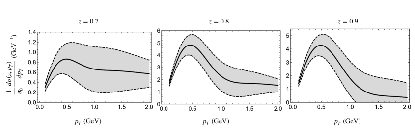
Figure 4: TMD distribution for a possible $b$-flavored heavy-light hadron inside a hemisphere jet in $e^{+}e^{-}$ collisions. For simplicity, we have short-written $z_{H}$ and $p_{T}^{H}$ as $z$ and $p_{T}$ respectively. The center of mass energy of the collision $Q=100~{}\rm{GeV}$ and $b_{\rm max}=2~{}\mathrm{GeV}^{-1}$.

In Fig. 4 we show TMD distributions of single $b$-flavored heavy-light hadron inside a hemisphere jet in $e^{+}e^{-}$ collisions (and not specified the $b$-hadron so $N_{H}$ in Eq. (84) is set to 1), with energy fraction $z_{H}$ carried by the heavy hadron fixed. The error bands come from varying each characteristic scale $\mu_{i}(\nu_{i})$ that appears in Eq. (143) up to $2\mu_{i}(2\nu_{i})$ and down to $\mu_{i}/2(\nu_{i}/2)$, and summing the errors from all the scale variations by quadrature. As $p_{T}^{H}$ approaches $0$, the error bands get narrower. This is because small $p_{T}$ lies in the non-perturbative region, and we simply freeze out the scale variations in those regions. That is, we only estimate the error from our perturbative computations, since we do not have control of the error of non-perturbative origin. We put more details on how we treat the scale variations involving non-perturbative regions in Appendix D.

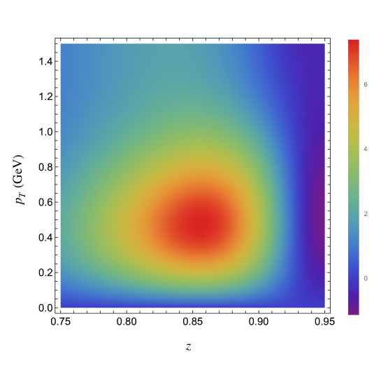
Figure 5: Two dimensional contour plot of $(z,p_{T})$ distribution for a b-flavored heavy-light hadron in a hemisphere jet in $e^{+}e^{-}$ collisions, according to the cross section Eq. (143) for numerical evaluations.

To have a better view of the joint $(z_{H},p_{T}^{H})$ distributions as displayed in Eq. (143), we made a two-dimensional contour plot shown in Fig. 5, where all the parameters are the same as those used in Fig. 4, using the central value of the scales. As shown in the contour plot, the dominant contributions come from the range roughly $z_{H}\in[0.8,0.9]$ and $p_{T}^{H}\in[0.3,0.7]~{}\rm GeV$. Even though the peak region is close to the nonperturbative domain, hence we need more sophisticated parameterization and study of the hadronization, we suspect that the shape of the distribution in Fig. 5 show some characteristics for a heavy-light hadron with a $b$ quark. Note that in Fig. 5, some negative values appear near the right edge of the plot, which needs more clarified studies on hadronization effects because they too close to the non-perturbative region. For instance, $z=0.95$ means that the residual scale for a $B$ meson $(1-z)m_{B}$ is around $0.25$ GeV.

7 Conclusions

In this paper, we study the heavy quark (HQ) mass effects to the transverse momentum dependent fragmentation function (TMDFF) using SCET. We start by calculating the one-loop contribution to the TMDFF that is initiated by a heavy quark. The resulting function is IR finite. While the IR dependence of the HQ TMDFF is different than the light quark case, the UV divergence comes from the virtual contribution, and thus is the same as found in the light TMDFF. The rapidity divergence comes from the zero-bin subtraction, and thus is also the same as the light TMDFF.

Given the possible hierarchy of scales between $q_{\perp}$ and $m$, where $q_{\perp}$ is the transverse momentum of the initiating parton with respect to hadron and $m$ is the heavy quark mass, we investigate the HQ TMDFF in the limit $q_{\perp}\ll m$. This is done by matching onto boosted heavy quark effective theory. This allows us to factorize the HQ TMDFF further into a shape function and a matching coefficient, which is done at one-loop order. We next study the opposite limit, $q_{\perp}\gg m$. In this case, we integrate out the fluctuations of $q_{\perp}$ and match onto the standard heavy quark fragmentation function. This is again done at one-loop. Finally, since the nonperturbative effects are always important when describing the hadronization of the final state hadron, we also include the nonperturbative fragmentation function, using a model previously introduced in the literature.

Using the above results, we study two different applications. First we study the heavy quark TMD jet fragmentation function (JFF), which describes a heavy quark fragmenting to a jet, where inside the jet is an observed heavy hadron. By studying this process, we may gain useful information of the hadronization of the heavy quark. When $q_{\perp}$ is much smaller than the jet scale, we can further factorize the HQ TMD JFF into the standard FF and what we define as the JFF module, containing the transverse momentum dependence. The JFF module can be factored into a hard function, a soft function, and the HQ TMDFF. We resum leading large logarithms (not including nonglobal logarithms) in the JFF module to NNL order.

As a second application, we investigate the heavy hadron TMD distribution with respect to the thrust axis in $e^{+}e^{-}$ annihilation. The results can be resummed using the HQ TMD JFF we obtained and numerical results are shown. In order to produce sensible results, we have a better handle on the nonperturbative region, but a more in depth study is beyond the scope of this paper.

Appendix A NLO result of the heavy quark TMDFF at parton frame

In the parton frame where the initiating parton is taken to have zero transverse momentum, the heavy quark TMDFF is given by

$$\mathcal{D}_{H/\mathcal{Q}}(z,{\bf{p}}_{\perp},\mu,\nu)=\sum_{X}\frac{1}{2N_{c}z}\mathrm{Tr}\langle 0|\delta\left(\frac{p_{+}}{z}-\mathcal{P}_{+}\right)\delta^{(D-2)}({\boldsymbol{\mathcal{P}}}_{\perp})\frac{{\overline{n}}\!\!\!/}{2}\Psi_{n}^{\mathcal{Q}}|H(p)X\rangle\langle H(p)X|\bar{\Psi}_{n}^{\mathcal{Q}}|0\rangle.$$ (148)

Here the derivative operator returns the transverse momentum of the initial parton expressed as ${\boldsymbol{\mathcal{P}}}_{\perp}={\bf{p}}_{\perp}+{\bf{p}}^{\perp}_{X}=0$. In this case the fragmentation function is the distribution of the transverse momentum for the observed hadron, ${\bf{p}}_{\perp}$, which, as introduced in Eq. (2), is related to the transverse momentum of the initial parton in the hadron frame by ${\bf{q}}_{\perp}^{2}={\bf{p}}_{\perp}^{2}/z^{2}$. We have the following explicit relation between the fragmentation functions in the parton and at the hadron frames :

$$\int d^{D-2}{\bf{p}}_{\perp}\mathcal{D}_{H/f}(z,{\bf{p}}_{\perp})=\int d^{D-2}{\bf{q}}_{\perp}D_{H/f}(z,{\bf{q}}_{\perp}).$$ (149)

This relation holds for any flavor of parton $f$.

Similar to how we obtained the NLO result of the fragmentation function at hadron frame, we can compute the NLO correction to the fragmentation function in the parton frame. The bare one-loop result in momentum space is

$$\mathcal{D}_{\mathcal{Q}/\mathcal{Q}}^{(1)}(z,{\bf{p}}_{\perp},\mu,\nu) = \frac{\alpha_{s}C_{F}}{2\pi^{2}}\Biggl{\{}\delta(1-z)\delta({\bf{p}}_{\perp}^{2})\Biggl{[}\Bigl{(}\frac{2}{\eta}+2\ln\frac{\nu}{p_{+}}+\frac{3}{2}\Bigr{)}\Bigl{(}\frac{1}{\epsilon_{\mathrm{UV}}}+\ln\frac{\mu^{2}}{\Lambda^{2}}\Bigr{)}+2$$

$$-\ln(1+\lambda)-\frac{2}{\sqrt{\lambda}}\arctan{\sqrt{\lambda}}-\mathrm{Li}_{2}(-\lambda)\Biggr{]}-\delta({\bf{p}}_{\perp}^{2})\Biggl{[}\frac{P_{qq}(z)}{C_{F}}\ln\lambda$$

$$+\left(\frac{2z}{1-z}\Bigl{(}\ln\frac{1+(1-z)^{2}\lambda}{(1-z)^{2}}-\frac{1}{1+(1-z)^{2}\lambda}\Bigr{)}\right)_{+}+(1-z)\ln\frac{1+(1-z)^{2}\lambda}{(1-z)^{2}}\Biggr{]}$$

$$-\Bigl{(}\frac{2}{\eta}+2\ln\frac{\nu}{p_{+}}+\frac{3}{2}\Bigr{)}\delta(1-z)\left(\frac{1}{{\bf{p}}_{\perp}^{2}}\right)_{\Lambda^{2}}+\frac{P_{qq}(z)}{C_{F}}\left(\frac{1}{{\bf{p}}_{\perp}^{2}+(1-z)^{2}m^{2}}\right)_{\Lambda^{2}}$$

$$-2z(1-z)\left(\frac{m^{2}}{({\bf{p}}_{\perp}^{2}+(1-z)^{2}m^{2})^{2}}\right)_{\Lambda^{2}}\Biggr{\}}.$$

Here the rapidity and UV divergences are the same as for the fragmentation function at hadron frame.

In impact-parameter space, the renormalized one-loop result is

$$\tilde{\mathcal{D}}_{\mathcal{Q}/\mathcal{Q}}(z,{\bf{b}};\mu,\nu) = \int d^{2}{\bf{p}}_{\perp}e^{i{\bf{b}}\cdot{\bf{p}}_{\perp}}\mathcal{D}_{\mathcal{Q}/\mathcal{Q}}(z,{\bf{p}}_{\perp};\mu,\nu)$$

$$= 1+\frac{\alpha_{s}C_{F}}{2\pi}\Biggl{\{}\delta(1-z)\Bigl{[}\Bigl{(}2\ln\frac{\nu}{p_{+}}+\frac{3}{2}\Bigr{)}\ln\bar{b}^{2}\mu^{2}+\frac{1}{2}\ln\bar{b}^{2}m^{2}\Bigr{]}$$

$$+\Bigl{(}\frac{2z}{1-z}\Bigr{)}_{+}\Bigl{[}2K_{0}((1-z)mb)+2\ln(1-z)-1\Bigr{]}$$

$$+2(1-z)K_{0}((1-z)mb)-\Bigl{(}\frac{4z}{1-z}\ln(1-z)\Bigr{)}_{+}$$

$$-2z(1-z)\Bigl{[}\frac{bm}{1-z}K_{1}((1-z)mb)-\frac{1}{(1-z)^{2}}\Bigr{]}\Biggr{\}}\ .$$

Here $b\sim 1/p_{\perp}$. This result in the parton frame can be easily compared with the hadron frame result, Eq. (2), where $b\sim 1/q_{\perp}=z/p_{\perp}$. From the result of Eq. (2) with replacement $b\to zb$, we immediately obtain the result Eq. (A).

We can also consider the heavy quark fragmentation in the parton frame in the limit ${\bf{p}}_{\perp}\ll m$. In this case, the same factorization as Eq. (42) holds and the fragmentation function is given by

$$\mathcal{D}_{H/\mathcal{Q}}(z,{\bf{p}}_{\perp}\ll m,\mu,\nu)=C_{\mathcal{Q}}(m,\mu)S_{H}(z,{\bf{p}}_{\perp},\mu,\nu).$$ (152)

Note that the heavy quark shape function $S_{H}$ is the same as for the hadron frame, with the one-loop result at the parton level given in Eq. (3). As explained in Sec. 3, the fragmentation for the small $p_{\perp}$ region is actually described by the residual mode in bHQET, which contributes to only for the large $z$ region. Thus, at leading power of $1-z$, the transverse momenta for the parton and hadron frames can be identified,

$$|{\bf{q}}_{\perp}|=\frac{|{\bf{p}}_{\perp}|}{z}\sim|{\bf{p}}_{\perp}|.$$ (153)

Appendix B One loop calculation of the TMD csoft function

In this section we perform the one-loop calculation the TMD csoft function $S_{R}$ defined in Eq. (106), reproduced here for convenience

$$S_{R}({\bf{l}}_{\perp};\mu,\nu)=\frac{1}{N_{c}}\mathrm{Tr}~{}\langle 0|\tilde{Y}_{n,cs}Y_{\overline{n},cs}^{\dagger}\delta^{(2)}({\bf{l}}_{\perp}+\Theta_{in}\cdot{\boldsymbol{\mathcal{P}}}_{\perp})Y_{\overline{n},cs}\tilde{Y}_{n,cs}^{\dagger}|0\rangle.$$ (154)

As expressed in the argument of the delta function in Eq. (154), the csoft function returns a nonzero value of ${\bf{l}}_{\perp}$ only when at least one gluon is radiated inside of the jet, while the delta function becomes $\delta^{(2)}({\bf{l}}_{\perp})$ for gluons that are all radiated outside of the jet.

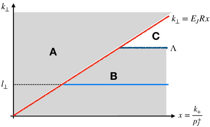
Figure 6: The phase space for real gluon emission for the calculation of the TMD csoft function $S_{R}$. The red line denotes the jet boundary, and the blue solid line in the region ‘B’ shows the contribution to the distribution with a nonzero $l_{\perp}~{}(|\equiv{\bf{l}}_{\perp}|)$.

In Fig. 6 we have illustrated the phase space for a real gluon emission for the one loop calculation. Here the csoft gluon momentum $k^{\mu}$ is power counted as shown in Eq. (96) and we consider the limit, $k_{\perp}~{}(\equiv|{\bf{k}}_{\perp}|)\ll E_{J}R$. Hence the largest momentum component $k_{+}$ should be much smaller than $p_{J}^{+}~{}(\sim 2E_{J})$ in the power counting, and the jet boundary can be approximated to be $k_{\perp}=E_{J}Rx$, where $x=k_{+}/p_{J}^{+}$. However, when integrating over $k$, the limit for $k_{+}$ can be set to be infinity, r since the momentum $p_{J}^{+}$ is to be considered infinitely larger than the csoft momentum.

When we consider the real gluon emission inside the jet, the transverse momentum is $l_{\perp}~{}(\equiv|{\bf{l}}_{\perp}|)$, and the amplitude is given by

$$M_{in}^{R}({\bf{l}}_{\perp}^{2})=\frac{\alpha_{s}C_{F}}{\pi^{2}}\frac{(\mu^{2}e^{\gamma_{E}})^{\epsilon}}{\Gamma(1-\epsilon)}\left(\frac{\nu}{p_{J}^{+}}\right)^{\eta}\Bigl{(}\frac{1}{{\bf{l}}_{\perp}^{2}}\Bigr{)}^{1+\epsilon}\int^{\infty}_{l_{\perp}/E_{J}R}dxx^{-1-\eta}\ ,$$ (155)

where we employed the rapidity regulator in order to handle the divergence as $x\to\infty$. $M_{in}^{R}$ has an IR divergence as ${\bf{l}}_{\perp}^{2}\to 0$, hence in order to regulate we use the $\Lambda^{2}$-distribution,

$$M_{in}^{R}({\bf{l}}_{\perp}^{2})=\Bigl{[}\int^{\Lambda^{2}}_{0}d{\bf{k}}_{\perp}^{2}M_{in}^{R}({\bf{k}}_{\perp}^{2})\Bigr{]}\delta({\bf{l}}_{\perp}^{2})+\Bigl{[}M_{in}^{R}({\bf{l}}_{\perp}^{2})\Bigr{]}_{\Lambda^{2}}\ .$$ (156)

The integration region of the first term with the delta function covers the region ‘B’ in the phase space shown in Fig. 6.

The out-jet region for real emission, where the amplitude is proportional to $\delta({\bf{l}}_{\perp}^{2})$, coincides with the region ‘A’ in Fig. 6. Therefore, if we combine the virtual contribution and the contributions from the integration of the regions ‘A’ and ‘B’, the net contribution becomes the result of the integration of the region ‘C’ with an overall negative sign since the virtual contribution covers the full phase space of Fig. 6 with the opposite sign. Thus, the net contribution proportional to $\delta({\bf{l}}_{\perp}^{2})$ is

$$\mathcal{M}_{\delta} =-\frac{\alpha_{s}C_{F}}{\pi^{2}}\frac{(\mu^{2}e^{\gamma_{E}})^{\epsilon}}{\Gamma(1-\epsilon)}\left(\frac{\nu}{p_{J}^{+}}\right)^{\eta}\int^{\infty}_{\Lambda/E_{J}R}dxx^{-1+\eta}\int^{x^{2}E_{J}^{2}R^{2}}_{\Lambda^{2}}d{\bf{k}}_{\perp}^{2}({\bf{k}}_{\perp}^{2})^{-1-\epsilon}$$

$$=\frac{\alpha_{s}C_{F}}{2\pi^{2}}\Bigl{[}\frac{1}{\epsilon^{2}}+\frac{1}{\epsilon}\ln\frac{\mu^{2}}{\Lambda^{2}}+\frac{1}{2}\ln^{2}\frac{\mu^{2}}{\Lambda^{2}}-\frac{\pi^{2}}{12}-2\Bigl{(}\frac{1}{\epsilon}+\ln\frac{\mu^{2}}{\Lambda^{2}}\Bigr{)}\Bigl{(}\frac{1}{\eta}+\ln\frac{\nu R}{2\Lambda}\Bigr{)}\Bigr{]}\ ,$$ (157)

where the $1/\epsilon$ poles are due to the UV divergences.

The remaining contribution for the one-loop calculation of $S_{R}$ is the second term in Eq. (156), i.e., the $\Lambda^{2}$ distribution of $M_{in}^{R}$ with nonzero ${\bf{l}}_{\perp}^{2}$, for which the integration region is denoted as the blue solid line in region ‘B’ of Fig. 6. Since ${\bf{l}}_{\perp}^{2}\neq 0$, $M_{in}^{R}$ is free from the IR divergence and is computed as

$$M_{in}^{R}({\bf{l}}_{\perp}^{2}\neq 0) =\frac{\alpha_{s}C_{F}}{\pi^{2}}\left(\frac{\nu}{p_{J}^{+}}\right)^{\eta}\frac{1}{{\bf{l}}_{\perp}^{2}}\int^{\infty}_{l_{\perp}/E_{J}R}dxx^{-1+\eta}$$

$$=\frac{\alpha_{s}C_{F}}{\pi^{2}}\frac{1}{{\bf{l}}_{\perp}^{2}}\Bigl{(}\frac{1}{\eta}+\frac{1}{2}\ln\frac{\nu^{2}R^{2}}{4{\bf{l}}_{\perp}^{2}}\Bigr{)}\ .$$ (158)

Combining the results of Eqs. (157) and (158), we obtain the one-loop result of the csoft function $S_{R}$ as

$$S_{R}^{(1)}({\bf{l}}_{\perp},\mu,\nu) =\frac{\alpha_{s}C_{F}}{2\pi^{2}}\Bigl{\{}\delta({\bf{l}}_{\perp}^{2})\Bigl{[}\frac{1}{\epsilon^{2}}+\frac{1}{\epsilon}\ln\frac{\mu^{2}}{\Lambda^{2}}+\frac{1}{2}\ln^{2}\frac{\mu^{2}}{\Lambda^{2}}-\frac{\pi^{2}}{12}-2\Bigl{(}\frac{1}{\epsilon}+\ln\frac{\mu^{2}}{\Lambda^{2}}\Bigr{)}\Bigl{(}\frac{1}{\eta}+\ln\frac{\nu R}{2\Lambda}\Bigr{)}\Bigr{]}$$

$$\hskip 56.9055pt+\Bigl{[}\frac{1}{{\bf{l}}_{\perp}^{2}}\Bigl{(}\frac{2}{\eta}+\ln\frac{\nu^{2}R^{2}}{4{\bf{l}}_{\perp}^{2}}\Bigr{)}\Bigr{]}_{\Lambda^{2}}\Bigr{\}}\ .$$ (159)

The renomalized result and the result in ${\bf{b}}$-space are presented in Eqs. (5.2) and (109), respectively. Furthermore, as discussed in Sec. 6, we can obtain the one-loop result of the TMD soft function with thrust axis by setting $R\to 2$.

Appendix C Implication of nonperturbative contributions for ${\bf{q}}_{\perp}\sim\Lambda_{\rm QCD}$

When ${\bf{q}}_{\perp}\sim\Lambda_{\rm QCD}$, the transverse momentum distribution becomes entirely nonperturbative. Since the heavy quark mass is taken to be much larger than ${\bf{q}}_{\perp}$, we can integrate out the degrees of freedom of the scale $p^{2}\sim m^{2}$ and obtain the heavy quark function $C_{Q}(m,\mu)$ before we consider the nonperturbative TMD function. Therefore the heavy quark TMD FF for ${\bf{q}}_{\perp}\sim\Lambda_{\rm QCD}$ can be written as

$$D_{H/\mathcal{Q}}(z,{\bf{q}}_{\perp}\sim\Lambda_{\rm QCD};\mu,\nu)=C_{\mathcal{Q}}(m,\mu)S_{H/\mathcal{Q}}(z,{\bf{q}}_{\perp}\sim\Lambda_{\rm QCD},\mu,\nu),$$ (160)

where $S_{H/\mathcal{Q}}$ has been introduced in Eq. (44) and in this case is totally nonperturbative.

The rapidity scale dependence in $S_{H/\mathcal{Q}}$ complicates any nonperturbative parameterization and its modeling. However, when we consider the whole scattering process, there will be another nonperturbative TMD soft function also with rapidity scale dependence. When combined with $S_{H/\mathcal{Q}}$, as seen in Eq. (114), the rapidity scale dependence can be removed. Therefore, for example, when we consider the nonperturbative TMD distribution of the HQTMD JFF studied in Sec. 5, it is useful to introduce a new function combining with $S_{R}$ in Eq. (106):

$$\tilde{\mathcal{S}}_{H/\mathcal{Q}}^{R}(z,{\bf{b}};\mu)=\tilde{S}_{R}({\bf{b}};\mu,\nu)\tilde{S}_{H/\mathcal{Q}}(z,{\bf{b}};m,\mu,\nu).$$ (161)

Although $\tilde{\mathcal{S}}_{H/\mathcal{Q}}^{R}$ is not dependent of the rapidity scale, it involves a large logarithm that comes from the rapidity gap between $\tilde{S}_{R}$ and $\tilde{S}_{H/Q}$,

$$\ln\frac{\nu_{cs}}{\nu_{r}}\approx\ln\frac{2q_{\perp}/R}{2E_{J}q_{\perp}/m}=\ln\frac{m}{E_{J}R},$$ (162)

where $\nu_{s}$ and $\nu_{r}$ are the characteristic rapidity scales of $\tilde{S}_{R}$ and $\tilde{S}_{H/Q}$, respectively, shown in Eq. (131). In the perturbative limit, resumming the large rapidity logarithms gives

$$\tilde{\mathcal{S}}_{H/\mathcal{Q}}^{R}(z,{\bf{b}};\mu)=\Bigl{(}\frac{\nu_{cs}}{\nu_{r}}\Bigr{)}^{2a_{\Gamma}(\mu,1/\bar{b})}\tilde{S}_{R}({\bf{b}};\mu,\nu_{s})\tilde{S}_{H/\mathcal{Q}}(z,{\bf{b}};m,\mu,\nu_{r}).$$ (163)

The $\mu$-evolution result for the combined function, $\tilde{\mathcal{S}}_{H/Q}^{R}$, is given by

$$\tilde{\mathcal{S}}_{H/\mathcal{Q}}^{R}(z,{\bf{b}};\mu)=U_{\mathcal{S}}^{R}(\mu,\mu_{0})\tilde{\mathcal{S}}_{H/\mathcal{Q}}^{R}(z,{\bf{b}};\mu_{0}),$$ (164)

where the evolution kernel at NLL is

$$\ln U^{R}_{\mathcal{S}}(\mu,\mu_{0})=\ln\frac{m^{2}}{E_{J}^{2}R^{2}}a_{\Gamma}(\mu,\mu_{0})-\frac{2C_{F}}{\beta_{0}}\ln\frac{\alpha_{s}(\mu)}{\alpha_{s}(\mu_{0})}\ .$$ (165)

Here, in order to guarantee a perturbative expansion, the lower scale $\mu_{0}$ must be chosen as some scale above $\Lambda_{\mathrm{QCD}}$, e.g., $\mu_{0}\sim 1~{}\mathrm{GeV}$. Then we can parameterize $\tilde{\mathcal{S}}_{H/\mathcal{Q}}^{R}(z,{\bf{b}};\mu_{0})$ as a genuine nonperturbative function.

When we consider heavy hadron fragmentation with respect to the thrust axis, studied in Sec. 6, following discussions in Refs. Collins:2011zzd ; Ebert:2019okf ; Kang:2020yqw , the nonpertubative TMD function can be defined as

$$\tilde{\mathcal{S}}_{H/\mathcal{Q}}^{rt}(z,{\bf{b}},\mu)=\tilde{S}_{rt}({\bf{b}},\mu,\nu)\tilde{S}_{H/\mathcal{Q}}(z,{\bf{b}},\mu,\nu).$$ (166)

Here the large rapidity logarithms are induced from the large gap between the characteristic scales $\nu_{r}$ and $\nu_{s}$, given by

$$\ln\frac{\nu_{s}}{\nu_{r}}\approx\ln\frac{q_{\perp}}{Qq_{\perp}/m}=\ln\frac{m}{Q}\ .$$ (167)

Similar to Eq. (163), the logarithms can be resummed as

$$\tilde{\mathcal{S}}_{H/\mathcal{Q}}^{rt}(z,{\bf{b}},\mu)=\Bigl{(}\frac{\nu_{cs}}{\nu_{r}}\Bigr{)}^{2a_{\Gamma}(\mu,1/\bar{b})}\tilde{S}_{rt}({\bf{b}},\mu,\nu_{s})\tilde{S}_{H/\mathcal{Q}}(z,{\bf{b}},\mu,\nu_{r}).$$ (168)

Finally, the $\mu$-evolution kernel between $\mu$ and $\mu_{0}~{}(\mu\gg\mu_{0})$ to NLL is given by

$$\ln U^{rt}_{\mathcal{S}}(\mu,\mu_{0})=\ln\frac{m^{2}}{Q^{2}}a_{\Gamma}(\mu,\mu_{0})-\frac{2C_{F}}{\beta_{0}}\ln\frac{\alpha_{s}(\mu)}{\alpha_{s}(\mu_{0})}\ .$$ (169)

Appendix D Scale variations for scales involving $1/\bar{b}$

For each characteristic scale involving $1/\bar{b}$, e.g. $\mu_{c}$ or $\mu_{cs}$ in Eq. (126), we vary it according to what shows in Figure 7 where we do what follows. First, $1/\bar{b}$ in the scale is replace with $1/(b^{*}\exp(\gamma_{E}/2))$, where $b^{*}$ is given in Eq. (144) and $\gamma_{E}$ the Euler–Mascheroni constant. We then introduce a simple scaling function

$$s(b)=\begin{cases}2-\frac{b}{b_{\rm max}}&\text{ if }b<b_{\rm max},\\ 1&\text{ if }b\geq b_{\rm max}\end{cases}$$ (170)

where $b_{\rm max}$ is the same as that appearing in defining $b^{*}$. Finally, the scale variation is carried out in the interval

$$\left(\frac{1}{s(b)b^{*}\exp(\gamma_{E}/2)},~{}\frac{s(b)}{b^{*}\exp(\gamma_{E}/2)}\right).$$ (171)

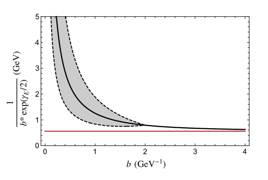
Figure 7: scale variations for characteristic scales involving $1/\bar{b}$. $b_{\rm max}=2$ in the plot (and also in Figure 4). The read line denotes the number $1/(b_{\rm max}\exp(\gamma_{E}/2))$, and it is the non-perturbative scale which $1/\bar{b}$ is frozen into (for $b_{\rm max}=2$, it is approximately equal to $0.56$ GeV).

References

- (1) R. Boussarie et al., TMD Handbook, arXiv:2304.03302.
- (2) J. C. Collins and D. E. Soper, Parton Distribution and Decay Functions, Nucl. Phys. B194 (1982) 445–492.
- (3) J. C. Collins, Fragmentation of transversely polarized quarks probed in transverse momentum distributions, Nucl. Phys. B 396 (1993) 161–182, [hep-ph/9208213].
- (4) A. Metz and A. Vossen, Parton Fragmentation Functions, Prog. Part. Nucl. Phys. 91 (2016) 136–202, [arXiv:1607.02521].
- (5) R. Bain, Y. Makris, and T. Mehen, Transverse Momentum Dependent Fragmenting Jet Functions with Applications to Quarkonium Production, JHEP 11 (2016) 144, [arXiv:1610.06508].
- (6) D. Neill, I. Scimemi, and W. J. Waalewijn, Jet axes and universal transverse-momentum-dependent fragmentation, JHEP 04 (2017) 020, [arXiv:1612.04817].
- (7) Z.-B. Kang, X. Liu, F. Ringer, and H. Xing, The transverse momentum distribution of hadrons within jets, JHEP 11 (2017) 068, [arXiv:1705.08443].
- (8) M. Boglione, J. O. Gonzalez-Hernandez, and R. Taghavi, Transverse parton momenta in single inclusive hadron production in annihilation processes, Phys. Lett. B 772 (2017) 78–86, [arXiv:1704.08882].
- (9) Belle Collaboration, R. Seidl et al., Transverse momentum dependent production cross sections of charged pions, kaons and protons produced in inclusive annihilation at 10.58 GeV, Phys. Rev. D 99 (2019), no. 11 112006, [arXiv:1902.01552].
- (10) M. Soleymaninia and H. Khanpour, Transverse momentum dependent of charged pion, kaon, and proton/antiproton fragmentation functions from annihilation process, Phys. Rev. D 100 (2019), no. 9 094033, [arXiv:1907.12294].
- (11) M. Boglione and A. Simonelli, Factorization of cross section, differential in , and thrust, in the -jet limit, JHEP 02 (2021) 076, [arXiv:2011.07366].
- (12) Z.-B. Kang, D. Y. Shao, and F. Zhao, QCD resummation on single hadron transverse momentum distribution with the thrust axis, JHEP 12 (2020) 127, [arXiv:2007.14425].
- (13) Y. Makris, F. Ringer, and W. J. Waalewijn, Joint thrust and TMD resummation in electron-positron and electron-proton collisions, JHEP 02 (2021) 070, [arXiv:2009.11871].
- (14) L. Gamberg, Z.-B. Kang, D. Y. Shao, J. Terry, and F. Zhao, Transverse polarization in collisions, Phys. Lett. B 818 (2021) 136371, [arXiv:2102.05553].
- (15) M. Boglione, J. O. Gonzalez-Hernandez, and A. Simonelli, Transverse momentum dependent fragmentation functions from recent BELLE data, Phys. Rev. D 106 (2022), no. 7 074024, [arXiv:2206.08876].
- (16) U. D’Alesio, L. Gamberg, F. Murgia, and M. Zaccheddu, Transverse polarization in processes within a TMD factorization approach and the polarizing fragmentation function, JHEP 12 (2022) 074, [arXiv:2209.11670].
- (17) M. Boglione and A. Simonelli, Full treatment of the thrust distribution in single inclusive → h X processes, JHEP 09 (2023) 006, [arXiv:2306.02937].
- (18) M. Dasgupta and G. P. Salam, Resummation of nonglobal QCD observables, Phys. Lett. B512 (2001) 323–330, [hep-ph/0104277].
- (19) A. Banfi, G. Marchesini, and G. Smye, Away from jet energy flow, JHEP 08 (2002) 006, [hep-ph/0206076].
- (20) J. Collins, Foundations of perturbative QCD, vol. 32. Cambridge University Press, 11, 2013.
- (21) S. M. Aybat and T. C. Rogers, TMD Parton Distribution and Fragmentation Functions with QCD Evolution, Phys. Rev. D 83 (2011) 114042, [arXiv:1101.5057].
- (22) J.-y. Chiu, A. Jain, D. Neill, and I. Z. Rothstein, The Rapidity Renormalization Group, Phys. Rev. Lett. 108 (2012) 151601, [arXiv:1104.0881].
- (23) J.-Y. Chiu, A. Jain, D. Neill, and I. Z. Rothstein, A Formalism for the Systematic Treatment of Rapidity Logarithms in Quantum Field Theory, JHEP 05 (2012) 084, [arXiv:1202.0814].
- (24) M. G. Echevarría, A. Idilbi, and I. Scimemi, Soft and Collinear Factorization and Transverse Momentum Dependent Parton Distribution Functions, Phys. Lett. B 726 (2013) 795–801, [arXiv:1211.1947].
- (25) M. A. Ebert, I. W. Stewart, and Y. Zhao, Towards Quasi-Transverse Momentum Dependent PDFs Computable on the Lattice, JHEP 09 (2019) 037, [arXiv:1901.03685].
- (26) Y. Makris and V. Vaidya, Transverse Momentum Spectra at Threshold for Groomed Heavy Quark Jets, JHEP 10 (2018) 019, [arXiv:1807.09805].
- (27) R. F. del Castillo, M. G. Echevarria, Y. Makris, and I. Scimemi, TMD factorization for dijet and heavy-meson pair in DIS, JHEP 01 (2021) 088, [arXiv:2008.07531].
- (28) R. F. del Castillo, M. G. Echevarria, Y. Makris, and I. Scimemi, Transverse momentum dependent distributions in dijet and heavy hadron pair production at EIC, JHEP 03 (2022) 047, [arXiv:2111.03703].
- (29) R. von Kuk, J. K. L. Michel, and Z. Sun, Transverse momentum distributions of heavy hadrons and polarized heavy quarks, JHEP 09 (2023) 205, [arXiv:2305.15461].
- (30) C. W. Bauer, S. Fleming, and M. E. Luke, Summing Sudakov logarithms in in effective field theory, Phys. Rev. D63 (2000) 014006, [hep-ph/0005275].
- (31) C. W. Bauer, S. Fleming, D. Pirjol, and I. W. Stewart, An Effective field theory for collinear and soft gluons: Heavy to light decays, Phys. Rev. D63 (2001) 114020, [hep-ph/0011336].
- (32) C. W. Bauer, D. Pirjol, and I. W. Stewart, Soft collinear factorization in effective field theory, Phys. Rev. D65 (2002) 054022, [hep-ph/0109045].
- (33) C. W. Bauer, S. Fleming, D. Pirjol, I. Z. Rothstein, and I. W. Stewart, Hard scattering factorization from effective field theory, Phys. Rev. D66 (2002) 014017, [hep-ph/0202088].
- (34) J. Chay and C. Kim, Consistent treatment of rapidity divergence in soft-collinear effective theory, JHEP 03 (2021) 300, [arXiv:2008.00617].
- (35) A. V. Manohar and I. W. Stewart, The Zero-Bin and Mode Factorization in Quantum Field Theory, Phys. Rev. D76 (2007) 074002, [hep-ph/0605001].
- (36) A. K. Leibovich, Z. Ligeti, and M. B. Wise, Comment on quark masses in SCET, Phys. Lett. B564 (2003) 231–234, [hep-ph/0303099].
- (37) I. Z. Rothstein, Factorization, power corrections, and the pion form-factor, Phys. Rev. D70 (2004) 054024, [hep-ph/0301240].
- (38) J. Chay, C. Kim, and A. K. Leibovich, Quark mass effects in the soft-collinear effective theory and in the endpoint region, Phys. Rev. D72 (2005) 014010, [hep-ph/0505030].
- (39) C. Kim, Exclusive heavy quark dijet cross section, J. Korean Phys. Soc. 77 (2020), no. 6 469–476, [arXiv:2008.02942].
- (40) L. Dai, C. Kim, and A. K. Leibovich, Heavy quark jet production near threshold, JHEP 09 (2021) 148, [arXiv:2104.14707].
- (41) M. Beneke, G. Finauri, K. K. Vos, and Y. Wei, QCD light-cone distribution amplitudes of heavy mesons from boosted HQET, JHEP 09 (2023) 066, [arXiv:2305.06401].
- (42) S. Fleming, A. H. Hoang, S. Mantry, and I. W. Stewart, Top Jets in the Peak Region: Factorization Analysis with NLL Resummation, Phys. Rev. D 77 (2008) 114003, [arXiv:0711.2079].
- (43) M. Neubert, Factorization analysis for the fragmentation functions of hadrons containing a heavy quark, arXiv:0706.2136.
- (44) M. Fickinger, S. Fleming, C. Kim, and E. Mereghetti, Effective field theory approach to heavy quark fragmentation, JHEP 11 (2016) 095, [arXiv:1606.07737].
- (45) B. Mele and P. Nason, The Fragmentation function for heavy quarks in QCD, Nucl. Phys. B361 (1991) 626–644. [Erratum: Nucl. Phys.B921,841(2017)].
- (46) S. Mantry and F. Petriello, Factorization and Resummation of Higgs Boson Differential Distributions in Soft-Collinear Effective Theory, Phys. Rev. D 81 (2010) 093007, [arXiv:0911.4135].
- (47) M. Procura, W. J. Waalewijn, and L. Zeune, Resummation of Double-Differential Cross Sections and Fully-Unintegrated Parton Distribution Functions, JHEP 02 (2015) 117, [arXiv:1410.6483].
- (48) P. Nason and C. Oleari, A Phenomenological study of heavy quark fragmentation functions in e+ e- annihilation, Nucl. Phys. B 565 (2000) 245–266, [hep-ph/9903541].
- (49) M. Cacciari, P. Nason, and C. Oleari, A Study of heavy flavored meson fragmentation functions in e+ e- annihilation, JHEP 04 (2006) 006, [hep-ph/0510032].
- (50) M. Cacciari, G. P. Salam, and G. Soyez, The Anti-k(t) jet clustering algorithm, JHEP 04 (2008) 063, [arXiv:0802.1189].
- (51) S. D. Ellis, C. K. Vermilion, J. R. Walsh, A. Hornig, and C. Lee, Jet Shapes and Jet Algorithms in SCET, JHEP 11 (2010) 101, [arXiv:1001.0014].
- (52) Z.-B. Kang, F. Ringer, and I. Vitev, The semi-inclusive jet function in SCET and small radius resummation for inclusive jet production, JHEP 10 (2016) 125, [arXiv:1606.06732].
- (53) L. Dai, C. Kim, and A. K. Leibovich, Fragmentation of a Jet with Small Radius, Phys. Rev. D94 (2016), no. 11 114023, [arXiv:1606.07411].
- (54) L. Dai, C. Kim, and A. K. Leibovich, Heavy Quark Jet Fragmentation, JHEP 09 (2018) 109, [arXiv:1805.06014].
- (55) W. M.-Y. Cheung, M. Luke, and S. Zuberi, Phase Space and Jet Definitions in SCET, Phys. Rev. D80 (2009) 114021, [arXiv:0910.2479].
- (56) X. Liu and F. Petriello, Resummation of jet-veto logarithms in hadronic processes containing jets, Phys. Rev. D 87 (2013), no. 1 014018, [arXiv:1210.1906].
- (57) J. Chay, C. Kim, and I. Kim, Factorization of the dijet cross section in electron-positron annihilation with jet algorithms, Phys. Rev. D92 (2015), no. 3 034012, [arXiv:1505.00121].
- (58) J. Chay, C. Kim, Y. G. Kim, and J.-P. Lee, Soft Wilson lines in soft-collinear effective theory, Phys. Rev. D71 (2005) 056001, [hep-ph/0412110].
- (59) Z.-B. Kang, F. Ringer, and W. J. Waalewijn, The Energy Distribution of Subjets and the Jet Shape, JHEP 07 (2017) 064, [arXiv:1705.05375].
- (60) G. P. Korchemsky and A. V. Radyushkin, Renormalization of the Wilson Loops Beyond the Leading Order, Nucl. Phys. B283 (1987) 342–364.
- (61) I. A. Korchemskaya and G. P. Korchemsky, On lightlike Wilson loops, Phys. Lett. B287 (1992) 169–175.
- (62) J. C. Collins, D. E. Soper, and G. F. Sterman, Transverse Momentum Distribution in Drell-Yan Pair and W and Z Boson Production, Nucl. Phys. B 250 (1985) 199–224.
- (63) P. Sun, J. Isaacson, C. P. Yuan, and F. Yuan, Nonperturbative functions for SIDIS and Drell–Yan processes, Int. J. Mod. Phys. A 33 (2018), no. 11 1841006, [arXiv:1406.3073].
- (64) Z.-B. Kang, A. Prokudin, P. Sun, and F. Yuan, Extraction of Quark Transversity Distribution and Collins Fragmentation Functions with QCD Evolution, Phys. Rev. D 93 (2016), no. 1 014009, [arXiv:1505.05589].
- (65) M. A. Ebert, J. K. L. Michel, I. W. Stewart, and Z. Sun, Disentangling long and short distances in momentum-space TMDs, JHEP 07 (2022) 129, [arXiv:2201.07237].