concrete: Targeted Estimation of Survival and Competing Risks Estimands in Continous Time

Abstract

This article introduces the R package concrete, which implements a recently developed targeted maximum likelihood estimator (TMLE) for the cause-specific absolute risks of time-to-event outcomes measured in continuous time. Cross-validated Super Learner machine learning ensembles are used to estimate propensity scores and conditional cause-specific hazards, which are then targeted to produce robust and efficient plug-in estimates of the effects of static or dynamic interventions on a binary treatment given at baseline quantified as risk differences or risk ratios. Influence curve-based asymptotic inference is provided for TMLE estimates and simultaneous confidence bands can be computed for target estimands spanning multiple multiple times or events. In this paper we review the one-step continuous-time TMLE methodology as it is situated in an overarching causal inference workflow, describe its implementation, and demonstrate the use of the package on the PBC dataset.

 Introduction

In biomedical applications evaluating treatment effects on time-to-event outcomes, study subjects are often susceptible to competing risks such as all-cause mortality. In recent decades, several competing risk methods have been developed; including the Fine-Gray subdistributions model (Fine and Gray, 1999), cause-specific Cox regression (Benichou and Gail, 1990), pseudovalue (Klein and Andersen, 2005), and direct binomial (Scheike et al., 2008; Gerds et al., 2012) regressions; and authors have consistently cautioned against the use of standard survival estimands for causal questions involving competing risks. Nevertheless, reviews of clinical literature (Koller et al., 2012; Austin and Fine, 2017) found that most trials still fail to adequately address the effect of potential competing risks in their studies. Meanwhile, formal causal inference frameworks (Rubin, 1974; Pearl et al., 2016) gained recognition for their utility in translating clinical questions into statistical analyses and the targeted maximum likelihood estimation (TMLE) (Laan and Rubin, 2006; Laan and Rose, 2011, 2018) methodology developed from the estimating equation and one-step estimator lineage of constructing semi-parametric efficient estimators through solving efficient influence curve equations. The targeted learning roadmap (Petersen and van der Laan, 2014) combines these developments into a cohesive causal inference workflow and provides a structured way to think about statistical decisions. In this paper we apply the targeted learning roadmap to an analysis of time-to-event outcomes and demonstrate the R package concrete, which implements a recently developed continuous-time TMLE targeting cause-specific absolute risks (Rytgaard and van der Laan, 2021, 2022; Rytgaard et al., 2023).

Given identification and regularity assumptions, concrete can be used to efficiently estimate the treatment effect of interventions given at baseline. In short, the implemented one-step TMLE procedure consists of three stages: 1) an initial estimation of nuisance parameters, 2) a targeted update of the initial estimators to solve the estimating equation corresponding to the target statistical estimand’s efficient influence curve (EIC), and 3) a plug-in of the updated estimators into the original parameter mapping to produce a substitution estimator of the target estimand.

In concrete the initial nuisance parameter estimation is performed using Super Learning, a cross-validated machine-learning ensemble algorithm with asymptotic oracle guarantees (Laan and Dudoit, 2003; Laan et al., 2007; Polley et al., 2021), as flexible machine-learning approaches such as Super Learners with robust candidate libraries and appropriate loss functions often give users the best chance of achieving the convergence rates needed for TMLE’s asymptotic properties. The subsequent targeted update is based on semi-parametric efficiency theory in that efficient regular and asymptotically linear (RAL) estimators must have influence curves equal to the efficient influence curve (EIC) of the target statistical estimand, see e.g. (Bickel et al., 1998; Laan and Rose, 2011, 2018; Kennedy, 2016). In TMLE, initial nuisance parameter estimates are updated to solve the estimating equation corresponding to the target EIC, thus recovering normal asymptotic inference (given that initial estimators converge at adequate rates) while leveraging flexible machine-learning algorithms for initial estimation. In Section 2.3 we outline how Super Learner is used to estimate nuisance parameters in concrete; more detailed guidance on how to best specify Super Learner estimators is provided in e.g., (Phillips et al., 2023; Dudoit and van der Laan, 2005; Vaart et al., 2006). Section 2.3 outlines the subsequent targeted update which is fully described in (Rytgaard and van der Laan, 2021).

Currently concrete can be used to estimate estimands derived from cause-specific absolute risks (e.g., risk ratios and risk differences) under static and dynamic interventions on binary treatments given at baseline. Estimands can be jointly targeted at multiple times, up to full risk curves over an interval, and for multiple events in cases with competing risks. Methods are available to handle right censoring, competing risks, and confounding by baseline covariates. Point estimates can be computed using g-formula plug-in or one-step TMLE, and asymptotic inference for the latter is derived from the variance of the efficient influence curve.

concrete is not intended to be used for data with clustering, left trunctation (i.e. delayed entry) or interval censoring. Currently the Super Learners for estimating conditional hazards must be comprised of Cox regressions (Cox, 1972) although the incorporation of hazard estimators based on penalized Cox regressions and highly adaptive lasso are planned in future package versions. Support for stochastic interventions and interventions on multinomial and continuous treatments are also forthcoming, while longitudinal methods to handle time-dependent treatment regimes and time-dependent confounding are in longer term development.

 A concrete example: analyzing the competing risks in the PBC dataset

Below we illustrate the usage of concrete on the well-known Mayo Clinic Primary Biliary Cholangitis (PBC) data set (Fleming and Harrington, 1991; Therneau and Grambsch, 2000). We estimate the cause-specific counterfactual absolute risk differences, i.e. average treatment effects, under two levels of a binary treatment (randomization to placebo or D-penicillamine). The treatment column "trt" is transformed so that 0 indicates placebo and 1 indicates D-penicillamine, and where the two competing events are transplant ("status"=1) and death ("status"=2) in the presence of right censoring ("status"=0). We include outcomes for two estimators, g-computation plug-in and TMLE, as well as point-wise 95% confidence intervals based on the estimated influence curves and 95% simultaneous confidence bands for the treatment effects across all targeted time points.

library(concrete)
data <- survival::pbc[, c("time", "status", "trt", "age", "sex", "albumin")]
data <- subset(data, subset = !is.na(data$trt))
data$trt <- data$trt - 1

# Specify Analysis
ConcreteArgs <- formatArguments(
    DataTable = data,
    EventTime = "time",
    EventType = "status",
    Treatment = "trt",
    Intervention = 0:1,
    TargetTime = 365.25/2 * (6:12),
    TargetEvent = 1:2,
    CVArg = list(V = 10),
    Verbose = FALSE
)

# Compute
ConcreteEst <- doConcrete(ConcreteArgs)

# Return Output
ConcreteOut <- getOutput(ConcreteEst, Estimand = "RD", Simultaneous = TRUE)
plot(ConcreteOut, NullLine = TRUE, ask = FALSE)

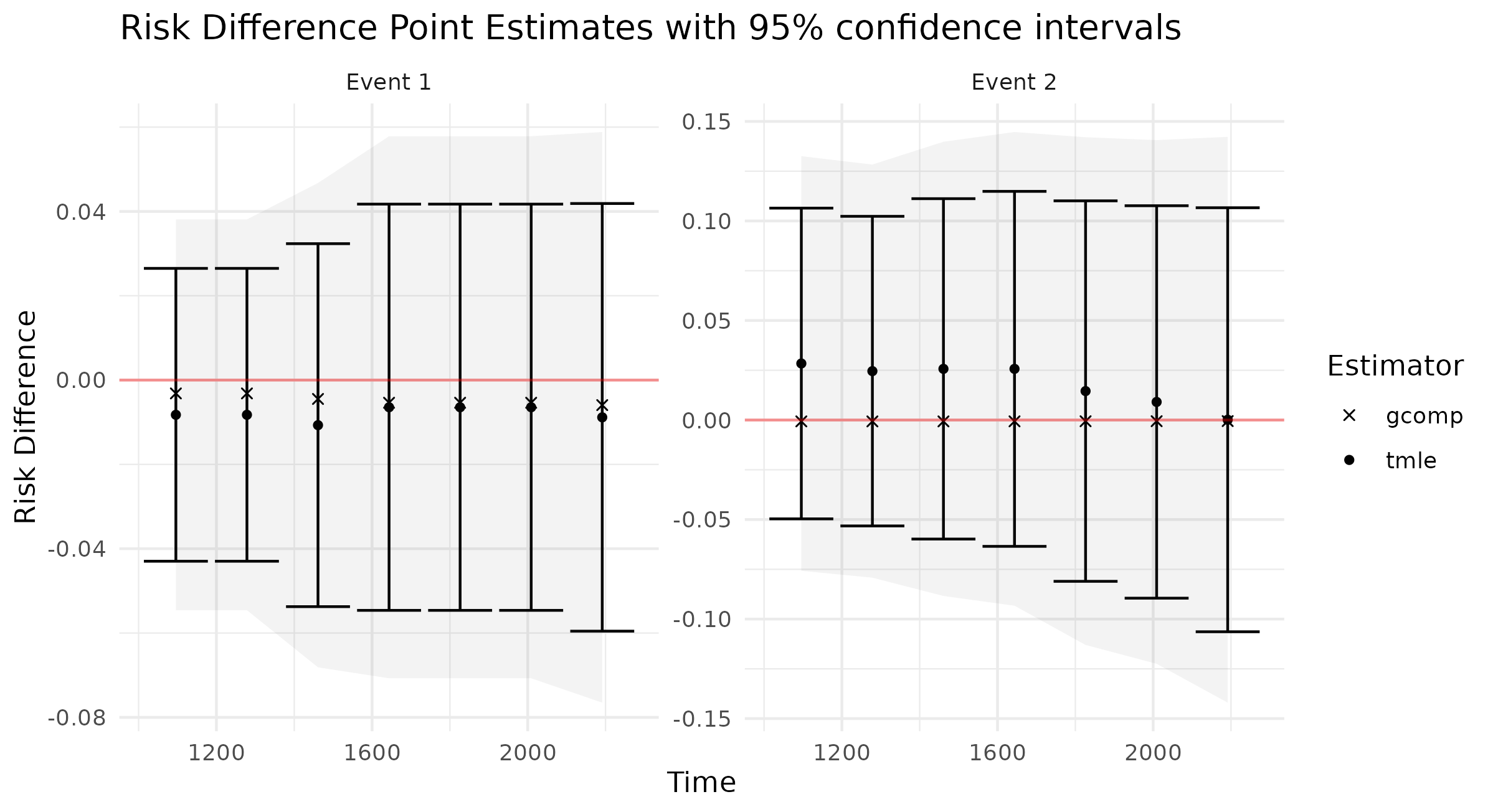
Figure 1: Estimated effect of D-penicillamine on the differences in cumulative incidence of the competing risks of transplant (Event 1) and death (Event 2) in the PBC dataset. Simultaneous 95% confidence bands are shown as gray ribbons. Error bars plot TMLE’s point-wise 95% confidence intervals. Null treatment effects are plotted as horizontal red lines.

 Other packages

concrete is the first R package on CRAN to implement a continuous-time TMLE for survival and competing risk estimands, but is related to existing R packages implementing semi-parametric efficient estimators for time-to-event-outcomes. The ltmle (Schwab et al., 2020), stremr (Sofrygin et al., 2017), and survtmle (Benkeser and Hejazi, 2019) implement discrete-time TMLEs for survival estimands and can be used to estimate right censored survival or competing risks estimands. Notably these packages all operate on a discrete underlying time scale and would thus require discretization of time-to-event data observed continuously; this discretization, if not performed optimally, negatively impacts both causal interpretation and estimator performance (Sofrygin et al., 2019; Ferreira Guerra et al., 2020; Sloma et al., 2021). ltmle and stremr use the method of iterated expectations while survtmle can employ the hazard-based TMLE formulation.

In addition, the CausalInference CRAN Task View lists riskRegression (Gerds et al., 2022) as estimating treatment effect estimands in survival settings using the inverse propensity of treatment weighted (IPTW) and double-robust augmented IPTW (AIPTW) estimators. None of the packages listed on the Survival CRAN Task View are described as implementing efficient semi-parametric estimators, though available via Github are the R packages adjustedCurves (Denz et al., 2023) and CFsurvival (Westling et al., 2021), which implement the AIPTW and a cross-fitted doubly-robust estimator respectively.

 Structure of this manuscript

This article is written for readers wishing to use the concrete package for their own analyses and for readers interested in an applied introduction to the one-step continuous-time TMLE method described in (Rytgaard and van der Laan, 2021). Section 2 outlines the targeted learning approach to time-to-event causal effect estimation, with subsection 2.3 providing details on our one-step TMLE implementation. Usage of the concrete package and its features is then provided in Section 3, continuing the above example of a simple competing risks analysis of the PBC dataset.

 The Targeted Learning framework for survival analysis

At a high level, the targeted learning roadmap for analyzing continuous-time survival or competing risks consists of:

1. Specifying the causal model and defining a causal estimand (e.g. causal risk difference). Considerations include defining a time zero and time horizon, specifying the intervention (i.e., treatment) variable and the desired interventions (including on sources of right censoring), and specifying the target time(s) and event(s) of interest.

2. Defining a statistical model and statistical estimand, and evaluating the assumptions necessary for the statistical estimand to identify the causal estimand. Considerations include identifying confounding variables, establishing positivity for desired interventions, and formalizing knowledge about the statistical model (e.g. dependency structures or functional structures).

3. Performing estimation and providing inference. Considerations include prespecification of an estimator and an inferential approach with desirable theoretical properties (e.g. consistency and efficiency within a desired class), and assessing via outcome-blind simulations the estimator’s robustness and suitability for the data at hand.

In the following sections we discuss these three stages in greater detail.

 The causal model: counterfactuals, interventions, and causal estimands

With time-to-event data, typical counterfactual outcomes are how long it would take for some event(s) to occur if subjects were hypothetically to receive some intervention, i.e. treatment. Let $A$ be the treatment variable and let $d$ be the hypothetical intervention rule of interest, i.e., the function that assigns treatment levels to each subject. The simplest interventions are static rules setting $A$ to some value $a$ in the space of treatment values $\mathcal{A}$, while more flexible dynamic treatment rules might assign treatments based on subjects’ baseline covariates (which we denote as $W$), and stochastic treatment rules incorporate randomness and may even depend on the natural treatment assignment mechanism in so-called modified treatment policies. Additionally, our goal in time-to-event analyses is often to assess the causal effect of some treatment rule $d$ on an event (or set of competing events) in the absence of right censoring. This "absence of right censoring" condition is in fact a static intervention to deterministically prevent right censoring, and is an implicit component to many interventions in time-to-event analyses.

Regardless of the type of intervention rule, the associated counterfactual survival data under intervention rule $d$, $X\sim P^{d}$, takes the general form

$$X=\left(T^{d},\,\Delta^{d},\,A^{d},W\right)$$ (1)

where $T^{d}\in(0,t_{max}]$ is the counterfactual time-to-event under intervention $d$ for the earliest of $J$ competing events up to some maximum follow-up time $t_{max}$, $\Delta^{d}\in\{1,\dots,J\}$ is the counterfactual event index indicating which the $J$ events would have hypothetically occurred first, and $A^{d}$ is the treatment variable under intervention $d$ (which for static and dynamic interventions will be a degenerate variable). Note that we differentiate between competing events (indexed $1,...,J$) and sources of right censoring (not present in $X$), as our goal is to assess the causal effect of treatment rule $d$ on the set of competing events in the absence of right censoring. For ideal experiments tracking just one event, i.e. $J=1$, the causal setting is one of survival of a single risk; if instead mutually exclusive events would be allowed to compete, then the causal setting is one with competing risks.

With the counterfactual data defined, causal estimands can then be specified as functions of the counterfactual data. For instance, if we were interested in effects of interventions $d_{0}$ versus $d_{1}$ on time-to-event outcomes, the counterfactual data $\tilde{X}\sim P^{\,0,1}$ might be represented as

$$\tilde{X}=\left(T^{d_{0}},\,\Delta^{d_{0}},\,A^{d_{0}},T^{d_{1}},\,\Delta^{d_{1}},\,A^{d_{1}},W\right)$$

We could then define estimands such as the causal event $j$ relative risks at time $t$

$$\tilde{\Psi}_{j,t}(P^{\,0,1})=\frac{{P}(T^{d_{1}}\leq t,\Delta^{d_{1}}=j)}{{P}(T^{d_{0}}\leq t,\Delta^{d_{0}}=j)}$$ (2)

These estimands may be of interest at a single timepoint, at multiple timepoints, or over a time interval, and in the case of competing risks may involve multiple events (e.g. $\tilde{\Psi}_{j,t}(P^{\,0,1}):t\in(0,t_{max}),\,j\in 1,\dots,J$). In any case, once the desired causal quantity of interest has been expressed as a function of the counterfactual data, efforts can then be made to identify the causal estimand with a function of observed data, i.e. a statistical estimand.

 Observed data, identification, and statistical estimands

Observed time-to-event data $O\sim P_{0}$ with $J$ competing events can be represented as:

$$O=\left(\widetilde{T},\,\widetilde{\Delta},\,A,\,W\right)$$ (3)

where $\widetilde{T}\in(0,t_{max}]$ is the earlier of the first event time $T$ or the right censoring time $C$, $\widetilde{\Delta}\in\{0,\dots,J\}$ indicates which event occurs (with 0 indicating right censoring), $A$ is the observed treatment and $W$ is the set of baseline covariates.

To link causal estimands such as Eq. (2) to statistical estimands, we need a set of identification assumptions to hold, informally: consistency, positivity, and conditional exchangeability (or their structural causal model analogs) . Readers can find a full discussion of these identification assumptions for absolute risk estimands in Section 3 of (Rytgaard and van der Laan, 2022). Given these assumptions, we can identify the cause-$j$ absolute risk at time $t$ under intervention $d$ using the g-computation formula (Robins, 1986) as

$$P(T^{d}\leq t,\Delta^{d}=j)=\mathbb{E}_{\mathcal{W}}\left[\int_{\mathcal{A}}\,F_{j}(t\mid a,\,{w})\,\pi^{*}(a\mid w)\,da\right]$$ (4)

where $\pi^{*}(a\mid w)$ is the treatment propensity implied by the intervention $d$. Here $F_{j}(t\mid a,\,{w})$ is the conditional cause-$j$ absolute risk

$$F_{j}(t\mid a,\,{w})=\int_{0}^{t}\lambda_{j}(s\mid a,\,{w})\,S(s\texttt{-}\mid a,\,{w})\,ds\;,$$

where the cause-$j$ conditional hazard function $\lambda_{j}$ is defined as

$$\lambda_{j}(t\mid a,\,{w})=\lim\limits_{h\to 0}\frac{1}{h}P(\widetilde{T}\leq t+h,\,\widetilde{\Delta}=j\mid\widetilde{T}\geq t,\,a,\,{w})\;,$$

and the conditional event-free survival probability is given by

$$S(t\mid a,\,{w})=\exp\left(-\int^{t}_{0}\sum\limits_{j=1}^{J}\lambda_{j}(s\mid a,\,{w})\,ds\right).$$ (5)

From Eq (4), it follows that we can identify the causal cause-$j$ relative risk (2) at time $t$ by

$$\Psi_{F_{j,t}}(P_{0})=\frac{\mathbb{E}_{\mathcal{W}}\left[\int_{\mathcal{A}}\,F_{j}(t\mid a,\,{w})\,\pi^{*}_{d_{1}}(a\mid w)\,da\right]}{\mathbb{E}_{\mathcal{W}}\left[\int_{\mathcal{A}}\,F_{j}(t\mid a,\,{w})\,\pi^{*}_{d_{0}}(a\mid w)\,da\right]}$$ (6)

where $\pi^{*}_{d_{0}}$ and $\pi^{*}_{d_{1}}$ represent the treatment propensities implied by treatment rules $d_{0}$ and $d_{1}$ respectively.

It should be noted that even without the identification assumptions for causal inference, statistical estimands such as Eq. (6) may still have valuable interpretations as standardized measures isolating the importance of the "intervention" variable (Laan, 2006).

 Targeted estimation

The TMLE procedure for estimands derived from cause-specific absolute risks begins with estimating the treatment propensity $\pi$, the conditional hazard of censoring $\lambda_{c}$ and the conditional hazards of events $\lambda_{j}\,:\;j=1,\dots,J$. In concrete these nuisance parameters are estimated using the Super Learner algorithm, which involves specifying a cross-validation scheme, compiling a library of candidate algorithms, and designating a cross-validation loss function and a Super Learner meta-learner.

Specifying a Super Learner

For a simple $V\text{-fold}$ cross-validation setup, let $Q_{n}=\{O_{i}\}_{i=1}^{n}\sim P_{n}$ be the observed $n$ i.i.d observations of $O\sim P_{0}$ and let $B_{n}\in\{1,...,V\}^{n}$ be a random vector that assigns the $n$ observations into $V$ validation folds. Then for each $v$ in $1,...,V$ we define a training set $Q^{\mathcal{T}}_{v}=\{O_{i}:B_{n}^{i}=v\}\sim P^{\mathcal{T}}_{v}$ and corresponding validation set $Q^{\mathcal{V}}_{v}=\{O_{i}:B_{n}^{i}\neq v\}\sim P^{\mathcal{V}}_{v}$.

Having specified a cross-validation scheme, the next steps are to construct the Super Learner candidate library, define an appropriate loss function, and select a Super Learner meta-learner. Super Learner libraries should be comprised of candidate algorithms that range in flexibility while respecting existing data-generating knowledge. For instance, candidate estimators should incorporate incorporate domain knowledge regarding covariates and interactions are predictive of outcomes. If the number independent observations $n$ is small compared to the number of covariates, then Super Learner libraries should contain fewer candidates and either incorporate native penalization, e.g. regularized Cox regression (coxnet) (Simon et al., 2011), or be paired with covariate screening algorithms. If, on the other hand, the number of independent observations is large compared to the number of covariates, then Super Learner libraries can include more algorithms including highly flexible non-parametric algorithms such as highly adaptive lasso (HAL). It should be noted that using HAL for initial nuisance parameter estimation can achieve the necessary convergence rates (Laan, 2017; Bibaut and van der Laan, 2019; Rytgaard et al., 2023) for TMLE to be efficient. Super Learner loss functions should imply a risk that is minimized by the true data-generating process and define a loss-based dissimilarity tailored to the target parameter and a discrete selector that selects the best performing candidate should be used as the Super Learner meta-learner (Laan et al., 2007). If computationally feasible, Super Learners using more flexible meta-learner algorithms can safely be nested as candidates within a larger Super Learner using a discrete meta-learner. Additional guidance on Super Learner specification is provided in (Phillips et al., 2023) and Chapter 3 of (Laan and Rose, 2011).

Currently the default cross-validation setup in concrete follows the guidelines laid out in (Phillips et al., 2023), with the number of cross-validation folds increasing with decreased sample size. The default number of folds ranges from leave-one-out cross validation (LOOCV) for datasets with fewer than 30 independent observations to 2-fold cross validation for datasets with over 10000 independent observations. Default Super Learner libraries are provided and will be detailed in the following sections, but should be amended to suit the data at hand and to incorporate subject matter knowledge.

Estimating treatment propensity

Let $\pi_{0}$ be the true conditional distribution of $A$ given ${W}$ (i.e. the treatment propensity), let $\mathcal{M}_{\pi}=\left\{\hat{\pi}:P_{n}\to\hat{\pi}(P_{n})\right\}$ be the library of candidate propensity score estimators, and let $L_{\pi}$ be a loss function such that the risk $\mathbb{P}_{0}\,L_{\pi}(\pi)\equiv\mathbb{E}_{0}\left[L_{\pi}(\pi,O)\right]$ is minimized by $\pi_{0}$. The discrete Super Learner estimator is then the candidate propensity estimator with minimal cross validated risk,

$$\hat{\pi}^{SL}=\operatorname*{argmin}_{\hat{\pi}\in\mathcal{M}_{\pi}}\sum_{v=1}^{V}\mathbb{P}_{Q^{\mathcal{V}}_{v}}\;L_{\pi}(\hat{\pi}(P^{\mathcal{T}}_{v}))$$ (7)

where $\hat{\pi}(P^{\mathcal{T}}_{v})$ are candidate propensity score estimators trained on data $Q^{\mathcal{T}}_{v}$. Currently concrete uses default SuperLearner (Polley et al., 2021) loss functions (non-negative least squares) and with a default Super Learner library consisting of elastic-net and extreme gradient boosting.

Estimating conditional hazards

For $\delta=0,\dots,J$ where ($\delta=0$) is censoring and ($\delta\in\{1,\dots,J\}$) are outcomes of interest, let $\lambda_{\delta}\,:\;\delta=0,\dots,J$ be the true conditional hazards, let $\mathcal{M}_{\delta}=\{\hat{\lambda}_{\delta}:P_{n}\to\hat{\lambda}_{\delta}(P_{n})\}$ be the libraries of candidate estimators, and let $L_{\delta}$ be loss functions such that the risks $\mathbb{P}_{0}\,L_{\delta}(\cdot)$ are minimized by the true conditional hazards $\lambda_{\delta}$. The discrete Super Learner selectors for each $\delta$ then chooses the candidate which has minimal cross validated risk

$$\hat{\lambda}_{\delta}^{SL}=\operatorname*{argmin}_{\hat{\lambda}_{\delta}\in\mathcal{M}_{\delta}}\sum_{v=1}^{V}\mathbb{P}_{Q^{\mathcal{V}}_{v}}\;L_{\delta}(\hat{\lambda}_{\delta}(P^{\mathcal{T}}_{v}))\;:\;\delta=0,\dots,J$$ (8)

where $\hat{\lambda}_{\delta}(P^{\mathcal{T}}_{v})$ are candidate event $\delta$ conditional hazard estimators trained on data $Q^{\mathcal{T}}_{v}$. The current concrete default is a library of two Cox models, treatment-only and main-terms, with cross-validated risk computed using negative log Cox partial-likelihood loss (Cox, 1975; Rytgaard and van der Laan, 2022)

$$\mathbb{P}_{Q^{\mathcal{V}}_{v}}\;L_{\delta}(\hat{\lambda}_{\delta}(P^{\mathcal{T}}_{v}))=\mathbb{P}_{Q^{\mathcal{V}}_{v}}\;L_{\delta}(\hat{\beta}_{\delta,Q^{\mathcal{T}}_{v}})=-\sum_{i:\,O_{i}\in Q^{\mathcal{V}}_{v}}\left[\hat{\beta}^{{}^{\prime}}_{\delta,Q^{\mathcal{T}}_{v}}\,W_{i}-\log\left[\sum_{i:\,O_{i}\in Q^{\mathcal{V}}_{v}}\mathbb{1}\left(\widetilde{T}_{l}\geq\widetilde{T}_{i}\right)\exp(\hat{\beta}^{{}^{\prime}}_{\delta,Q^{\mathcal{T}}_{v}}\,W_{h})\right]\right]\,$$

where $\mathcal{R}(t)$ is the risk set at time $t$, $\{h\,:\,\widetilde{T}_{h}\geq t\}$ and $\hat{\beta}_{\delta,Q^{\mathcal{T}}_{v}}$ are the coefficients of an event $\delta$ candidate Cox regression trained on data $Q^{\mathcal{T}}_{v}$.

Solving the efficient influence curve equation

For parameters such as risk ratios which are derived from cause-specific absolute risks, we solve a vector of absolute risk efficient influence curve (EIC) equations with one element for each combination of target event, target time, and intervention. That is, the EIC for a target parameter involving $J$ competing events, $K$ target times, and $M$ interventions is a $J\times K\times M$ dimensional vector where the component corresponding to the cause-specific risk of event $j$, at time $t_{k}$, and under intervention propensity $\pi^{*}_{m}$ is:

$$D^{*}_{m,j,k}(\lambda,\pi,S_{c})(O)=\sum_{l=1}^{J}\int\; h_{m,\,j,\,k,\,l,\,s}(\lambda,\pi,S_{c})(O)\,\left(N_{l}(s)-\mathbf{1}(\widetilde{T}\geq s)\,\lambda_{l}(s\mid A,\,{W})\right)\,ds$$ (9)

$${+\int_{\mathcal{A}}F_{j}(t_{k}\mid A=a,{W})\,\pi^{*}_{m}(a\mid{W})\,da-\Psi_{\pi^{*},j,t}(P_{0})}$$

where $N_{l}:l=0,\dots,J$ are the cause-specific counting processes

$$N_{l}(s)=\mathbf{1}\left\{\widetilde{T}\leq s,\widetilde{\Delta}=l\right\}$$

and $h_{m,\,j,\,k,\,l,\,s}(\lambda,\pi,S_{c})(O)$ is the TMLE "clever covariate"

$$h_{m,\,j,\,k,\,l,\,s} (\lambda,\pi,S_{c})(O)=\frac{{\color[rgb]{0,0,1}\pi^{*}_{m}(A\mid{W})\,}\mathbf{1}(s\leq t_{k})}{{\color[rgb]{0,0.7,0}\pi(A\mid{W})\;S_{c}(s\text{-}\mid A,\,{W})}}\,\bigg{(}\mathbf{1}(l=j)-\frac{{\color[rgb]{1,0,0}F_{j}(t_{k}\mid A,\,{W})}-{\color[rgb]{1,0,0}F_{j}(s\mid A,\,{W})}}{{\color[rgb]{1,0,0}S(s\mid A,\,{W})}}\bigg{)}$$ (10)

We highlight here that the clever covariate is a function of the intervention-defined treatment propensity, the observed intervention-related densities (i.e. the observed treatment propensity and cumulative conditional probability of remaining uncensored) which are unaffected by TMLE targeting, and the observed outcome-related densities which will be updated by TMLE targeting. Note also that our notation for the EIC ($D^{*}_{m,j,k}(\lambda,\pi,S_{c})(O)$) and clever covariate ($h_{m,\,j,\,k,\,l,\,s}(\lambda,\pi,S_{c})(O)$) reflects the dependence on $P$ through the cause-$j$ conditional hazards $\lambda=(\lambda_{l}\;:\;l=1,\dots,J)$ and the treatment propensity $\pi$ and conditional censoring survival $S_{c}(t\mid a,\,{w})=\exp\left(-\int^{t}_{0}\lambda_{0}(s\mid a,\,{w})\,ds\right)$.

The one-step continuous-time survival TMLE (Rytgaard and van der Laan, 2021) involves updating the cause-specific hazards $\lambda$ along the universally least favorable submodel, which is implemented as small recursive updates along a sequence of locally least favorable submodels. To describe this procedure, let us first introduce the following vectorized notation:

$${D}^{*} =\left(D^{*}_{m,j,k}:m=1,\dots,M\,,\;j=1,\dots,J\,,\;k=1,\dots,K\right)$$

$$h_{l,s} =\left(h_{m,\,j,\,k,\,l,\,s}:m=1,\dots,M\,,\;j=1,\dots,J\,,\;k=1,\dots,K\right)$$

The one-step continuous-time survival TMLE recursively updates the cause-specific hazards in the following manner: starting from $b=0$, with $\lambda^{0}_{j}=\hat{\lambda}^{SL}_{j}$, and $\lambda^{b}=\left(\lambda^{b}_{l}\;:\;l=1,\dots,J\right)$

$$\lambda^{b+1}_{l}=\lambda^{b}_{l}\,\exp\left(\frac{\left<\mathbb{P}_{n}{D}^{*}(\lambda^{b},\pi,S_{c})(O),\;h_{j,s}(\lambda^{b},\pi,S_{c})(O)\right>}{||\mathbb{P}_{n}{D}^{*}(\lambda^{b},\pi,S_{c})(O)||}\;\epsilon_{b}\right),\quad l=1,\dots,J$$ (11)

where

$$\left<x,y\right> =x^{\top}y\hskip 14.22636pt,\hskip 14.22636pt||x||=\sqrt{x^{\top}x}$$

and the step sizes $\epsilon_{b}$ are chosen such that

$$||\mathbb{P}_{n}{D}^{*}(\lambda^{b+1},\pi,S_{c})(O)||<||\mathbb{P}_{n}{D}^{*}(\lambda^{b},\pi,S_{c})(O)||$$

The recursive update following Eq (11) is completed at the iteration $B$ where

$$\left|\mathbb{P}_{n}{D}^{*}(\lambda^{B},\pi,S_{c})(O)\right|\leq\frac{\sqrt{\mathbb{P}_{n}{D}^{*}(\lambda^{B},\pi,S_{c})(O)^{2}}}{\sqrt{n}\,\log(n)}$$ (12)

This updated vector of conditional hazards $\lambda^{B}$ is then used to compute a plug-in estimate of the statistical estimand simultaneously across causes, target times, and interventions.

Estimating variance

In concrete, the variance of the TMLE is estimated based on the plug-in estimate of the sample variance of the EIC, $\frac{\mathbb{P}_{n}\;D^{*}(\hat{\lambda}^{B},\hat{}\pi,\hat{S}_{c})(O)^{2}}{n}$, which is a consistent estimator for the variance of the TMLE when all nuisance parameter estimators are consistent. In the presence of practical positivity violations arising from sparsity in finite samples (discussed further in Section 3.2), the EIC-based variance estimator can be anti-conservative and variance estimation by bootstrap may be more reliable (Tran et al., 2018). However, bias resulting from positivity violations cannot be remedied in this way, and so other methods of addressing positivity violations are recommended instead (Petersen et al., 2012). For multidimensional estimands, simultaneous confidence intervals can be computed by simulating the $1-\alpha$ quantiles of a multivariate normal distribution with the covariance structure of the estimand EICs.

 Using concrete

The basic concrete workflow consists of sequentially calling the following three functions:

• formatArguments()

• doConcrete()

• getOutput().

Users specify their estimation problem and desired analysis through formatArguments(), which checks the specified analysis for red flags and then produces a "ConcreteArgs" object. The "ConcreteArgs" object is then passed into doConcrete() which performs the specified continuous-time one-step survival TMLE and produces a "ConcreteEst" object which can be interrogated for diagnostics and estimation details. The "ConcreteEst" object can then be passed into getOutput() to produce tables and plots of cause-specific absolute risk derived estimands such as risk differences and relative risks.

 formatArguments()

The arguments of formatArguments() are primarily involved in specifying the observed data structure, the target estimand, and the TMLE estimator. The output, a "ConcreteArgs" object, contains the necessary elements of a continuous-time TMLE analysis.

ConcreteArgs <- formatArguments(
    DataTable = data,               # data.frame or data.table
    EventTime = "time",             # name of event time variable
    EventType = "status",           # name of event status variable
    Treatment = "trt",              # name of treatment variable
    ID = NULL,                      # name of the ID variable if present in input data
    Intervention = 0:1,             # 2 static interventions
    TargetTime = 365.25/2 * (6:12), # 7 target times: 3-6 years biannually
    TargetEvent = 1:2,              # 2 competing risks
    CVArg = list(V = 10),           # 10-Fold Cross-Validation
    Model = NULL,                   # using default Super Learner libraries
    Verbose = FALSE                 # less verbose warnings and progress messages
)

Data

The observed data are passed into the DataTable argument as either a data.frame or data.table object, which must contain columns corresponding to the observed time-to-event $\widetilde{T}$, the indicator of which event occured $\Delta$, and the treatment variable $A$. Treatment values in $A$ must be numeric, with binary treatments encoded as 0 and 1, and if the dataset contains a column with uniquely identifying subject IDs, its name should be passed into the ID argument. Any number of columns containing baseline covariates $W$ can also be included, but the data must be without missingness; imputation of missing covariates should be done prior to passing data into concrete while data with missing treatment or outcome values is not supported.

In the PBC example, the observed data is the data object, $\widetilde{T}$ is the column "time", $\Delta$ is the column "status", $A$ is the column "trt", and covariates $L$ are the remaining columns: ("age", "sex", and "albumin").

By default concrete pre-processes covariates using one-hot encoding to facilitate compatibility between candidate regression implementations which may process categorical variables differently. The "ConcreteArgs" object returned by formatArguments() includes the reformatted data as .[["DataTable"]] and the mapping of new covariate names to the originals can be retrieved by calling attr(.[["DataTable"]], "CovNames".

attr(ConcreteArgs[["DataTable"]], "CovNames")

#>    ColName CovName CovVal
#> 1:      L1     age      .
#> 2:      L2 albumin      .
#> 3:      L3     sex      f

This pre-processing can be turned off by setting RenameCovs = FALSE, which can be important for specifying dynamic interventions as will be discussed in the next section.

Target estimand: intervention, target events, and target times

Static interventions on a binary treatment $A$ setting all observations to $A=0$ or $A=1$ can specified with 0, 1, or c(0, 1) if both interventions are of interest, i.e. for contrasts such as risk ratios and risk differences. More complex interventions can be specified with a list containing a pair of functions: an "intervention" function which outputs desired treatment assignments and a "g.star" function which outputs desired treatment probabilities. These functions can take treatment and covariates as arguments and must produce treatment assignments and probabilities respectively, each with the same dimensions as the observed treatment. The function makeITT() creates list of functions corresponding to the binary treat-all and treat-none static interventions, which can be used as a template for specifying more complex interventions.

When specifying dynamic interventions using covariate names, it is important to set RenameCovs = FALSE, as otherwise concrete may rename covariates in the process of one-hot encoding categorical variables. "intervention" functions should take three inputs with the first being a data.table containing columns observed treatment values (here ObservedTrt), the second being a data.table of baseline covariates (here Covariates), and third being a data.table of propensity scores for the observed treatment values (here PropScore). The output of the "intervention" function should be a data.table with the same dimensions and names as the input observed treatment data.table, but containing the intervention treatment values instead. "g.star" functions take an additional fourth argument which should be a data.table of intervention treatment values (i.e. the output of the "intervention" function) and returns a data.table with one column containing the intervention propensity scores for each subject.

TreatOver60 <- list(
    "intervention" = function(ObservedTrt, Covariates, PropScore) {
        TrtNames <- colnames(ObservedTrt)
        Intervened <- data.table::copy(ObservedTrt)
        Intervened[, (TrtNames) := lapply(.SD, function(a) {
            as.numeric(Covariates[["age"]] > 60)
        }), .SDcols = TrtNames]
        return(Intervened)
    },
    # g.star function copied from from makeITT()
    "g.star" = function(Treatment, Covariates, PropScore, Intervened) {
        Probability <- data.table::data.table(1 * sapply(1:nrow(Treatment), function(i)
            all(Treatment[i, ] == Intervened[i, ])))
        return(Probability)
    }
)
TreatUnder60 <- list(
    "intervention" = function(ObservedTrt, Covariates, PropScore) {
        TrtNames <- colnames(ObservedTrt)
        Intervened <- data.table::copy(ObservedTrt)
        Intervened[, (TrtNames) := lapply(.SD, function(a) {
            as.numeric(Covariates[["age"]] <= 60)
        }), .SDcols = TrtNames]
        return(Intervened)
    }
    # if g.star function left empty, one will be copied from from makeITT()
)

ConcreteArgs <- formatArguments(
    DataTable = data,
    EventTime = "time",
    EventType = "status",
    Treatment = "trt",
    Intervention = list("Treat>60" = TreatOver60,
                        "Treat<=60" = TreatUnder60),
    TargetTime = 365.25/2 * (6:12),
    TargetEvent = 1:2,
    CVArg = list(V = 10),
    RenameCovs = FALSE, ## turn off covariate pre-processing ##
    Verbose = FALSE
)

The TargetEvent argument specifies the event types of interest. Event types must be be coded as integers, with non-negative integers reserved for censoring. If TargetEvent is left NULL, then all positive integer event types in the observed data will be jointly targeted. In the pbc dataset, there are 3 event values encoded by thestatus column: 0 for censored, 1 for transplant, and 2 for death. To analyze pbc with transplants treated as right censoring, TargetEvent should be set to 2, whereas for a competing risks analysis one could either leave TargetEvent = NULL or set TargetEvent = 1:2 as in the above example.

The TargetTime argument specifies the times at which the cause-specific absolute risks or event-free survival are estimated. Target times should be restricted to the time range in which target events are observed and formatArguments() will return an error if target time is after the last observed failure event time. If no TargetTime is provided, then concrete will target the last observed event time, though this is likely to result in a highly variable estimate if prior censoring is substantial. The TargetTime argument can either be a single number or a vector, as one-step TMLE can target cause-specific risks at multiple times simultaneously.

Estimator specification

The formatArguments() function can be used to modify the estimation procedure. The arguments of formatArguments() involved in estimation are the cross-validation setup CVArg, the Superlearner candidate libraries Model, the software backends PropScoreBackend and HazEstBackend, and the practical TMLE implementation choices MaxUpdateIter, OneStepEps, and MinNuisance. Note that Model is used in this section in line with common usage in statistical software, rather than to refer to formal statistical or causal models as in preceding sections.

Cross-validation is implemented using origami::make_folds() and using the input of the CVArg argument. If no input is provided into CVArg, the default cross-validation setup follows the recommendations in (Phillips et al., 2023). Cross-validation folds are stratified by event type and the number of folds ranges from 2 for datasets with greater than 10000 independent observations to LOOCV for datasets with fewer than 30 independent observations. Chapter 5 of the online Targeted Learning Handbook (Malenica et al., ) demonstrates the specification of several other cross-validation schemes.

Super Learner libraries for estimating nuisance parameters are specified through the Model argument. The input should be a named list with an element for the treatment variable and one for each event type including censoring as illustrated in the following code example. The list element corresponding to treatment must be named with the column name of the treatment variable, and the list elements corresponding to each event type must be named by the character which corresponds to the numeric value of the event type (e.g. "0" for censoring). Any missing specifications will be filled in with defaults, and the resulting list of libraries can be accessed in the output .[["Model"]] and further edited by the user, as shown below.

# specify regression models
ConcreteArgs$Model <- list(
    "trt" = c("SL.glmnet", "SL.bayesglm", "SL.xgboost", "SL.glm", "SL.ranger"),
    "0" = NULL, # will use the default library
    "1" = list(Surv(time, status == 1) ~ trt, Surv(time, status == 1) ~ .),
    "2" = list("Surv(time, status == 2) ~ trt", "Surv(time, status == 2) ~ .")
)

In concrete, propensity scores are by default estimated using the with candidate algorithms c("xgboost", "glmnet") implemented by packages xgboost (Chen et al., 2022) and glmnet (Friedman et al., 2010). For further details about these packages, see their respective package documentations.

For estimating the necessary conditional hazards, concrete currently relies on a discrete Superlearner consisting of a library of Cox models implemented by survival::coxph() evaluated on cross-validated partial-likelihood loss as detailed in Section 2.3. Support for estimation of hazards using coxnet (Simon et al., 2011), Poisson-HAL and other methods is planned in future package versions. The default Cox specifications are a treatment-only regression and a main-terms regression including treatment and all covariates. These models can be specified as strings or formulas as can be seen in the above example.

As detailed by Eq. (11) and (12), the one-step TMLE update step involves recursively updating cause-specific hazards, summing along small steps $\epsilon_{b}$. At default the maximum step size is 0.1, and is halved persistently whenever a step would increase the mean estimated EIC. The MaxUpdateIter argument is used to provide a definite stop to the recursive TMLE update. The default of 500 steps should be sufficient for most applications, but may need to be increased when targeting estimands with many components or for rare events. The presence of practical positivity sparsity can also result in slow TMLE convergence, but increasing MaxUpdateIter would not be not an adequate solution there as the resulting TMLE estimates and inference may still be unreliable. The MinNuisance argument can be used to specify a lower bound for the product of the propensity score and lagged survival probability for remaining uncensored; this term is present in the denominator of the efficient influence function and enforcing a lower bound decreases estimator variance at the cost of introducing bias but improving stability.

ConcreteArgs objects

The "ConcreteArgs" output of formatArguments() is an environment containing the estimation specification as objects that can be modified by the user. The modified "ConcreteArgs" object should then be passed back through formatArguments() to check the modified estimation specification.

# decrease the maximum tmle update number to 50
ConcreteArgs$MaxUpdateIter <- 50

# add a candidate regression with treatment interactions
ConcreteArgs[["Model"]][["2"]][[3]] <- "Surv(time, status == 2) ~ trt*."

# validate new estimation specification
ConcreteArgs <- formatArguments(ConcreteArgs)

"ConcreteArgs" objects can be printed to display summary information about the specified estimation problem,

print(ConcreteArgs, Verbose = FALSE)

Below, we can see that the specified analysis is for two competing risks (Target Events: 1, 2) under interventions "A=1" and "A=0" assigning all subjects to treated and control arms, respectively. Objects in the "ConcreteArgs" environment can be interrogated directly for details about any particular aspect of the estimation specification. For instance, as mentioned before the one-hot encoding of covariates can be seen in a table by attr(.[["DataTable"]], "CovNames"), intervention treatment assignments can be checked at .[["Regime]].

 doConcrete()

Adequately specified "ConcreteArgs" objects can then be passed into the doConcrete() function which will then perform the specified TMLE analysis. The output is an object of class "ConcreteEst" which contains TMLE point estimates and corresponding estimated influence curves for the cause-specific absolute risks for each targeted event at each targeted time under each intervention. If the GComp argument is set to TRUE, then a Super Learner-based g-formula plugin estimate of the targeted risks will be included in the output.

ConcreteEst <- doConcrete(ConcreteArgs)

We have reviewed the one-step continuous-time TMLE implementation in Section 2.3, so here we will name the non-exported functions in doConcrete() which perform each of the steps of the one-step continuous-time survival TMLE procedure, in case users wish to explore the implementation in depth.

The cross-validation (Section 2.3) is checked and evaluated in formatArguments(), returning fold assignments as the .[["CVFolds"]] element of the "ConcreteArgs" object.

The initial estimation of nuisance parameters and is performed by the function getInitialEstimate() which depends on getPropScore() for propensity scores (Section 2.3) and getHazEstimate() for the conditional hazards (Section 2.3).

Computing of EICs is done by getEIC() which is used within the doTmleUpdate() function which performs the one-step TMLE update procedure (Section 2.3).

ConcreteEst objects

The print method for "ConcreteEst" objects summarizes the estimation target and displays diagnostic information about TMLE update convergence, intervention-related nuisance parameter bounding, and the nuisance parameter Super Learners.

    print(ConcreteEst, Verbose = FALSE)

If TMLE has not converged, the mean EICs that have not attained the desired cutoff, i.e. Eq (11), will be displayed in a table. For instance, we can see above that the absolute value of the mean EIC for intervention ‘Treat>60’ at time 1461 for event 1 has not reached the stopping criteria and is $1.6$ times larger than the stopping criteria. Increasing the the maximum number of TMLE update iterations via MaxUpdateIter can allow TMLE to finish updating nuisance parameters, though at target time points when few events have yet occurred even small mean EIC values may not meet the convergence criteria and adequate convergence may require many iterations.

The extent to which the intervention-related nuisance parameters (i.e. propensity scores and probabilities of remaining uncensored) have been lower-bounded is also reported for each intervention both in terms of the percentage of nuisance weights that have been bounded and the percentage of subjects with bounded nuisance weights. If users suspect possible positivity issues, the plot method for "ConcreteEst" objects can be used to visualize the distribution of estimated propensity scores for each intervention, with the red vertical line marking the cutoff for lower-bounding.

    plot(ConcreteEst, ask  = FALSE)

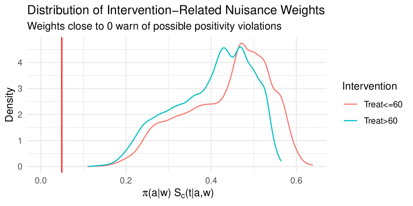
Figure 2:

Intervention-related nuisance parameters with values close to 0 indicate the possibility of positivity violations and may warrant re-examining the target time(s), interventions, and covariate adjustment sets. In typical survival applications, positivity issues may arise when targeting times at which some subjects are highly likely to have been censored, or if certain subjects are unlikely to have received a desired treatment intervention. As positivity violations not only impact causal interpretability, but also estimator behaviour, we urge users to re-consider their target analyses; (Petersen et al., 2012) provides guidance on reacting to positivity issues.

The last three tables ("Cens. 0", "Event 1", and "Event 2") in the above code output show the candidate estimators of nuisance parameters, summarized with the cross-validated risk of each candidate estimator followed by their weight in the corresponding Super Learners.

 getOutput()

getOutput() takes as an argument the "ConcreteEst" object returned by doConcrete() and can be used to produce tables and plots of the cause-specific risks, risk differences, and relative risks. By default getOutput() returns a data.table with point estimates and pointwise standard errors for cause-specific absolute risks, risk differences, and risk ratios. By default, the first listed intervention is used as the "treated" group while the second is considered "control"; other contrasts can be specified via the Intervention argument. Below we show a subset of the relative risk estimates produced by the "nutshell" estimation specification for the pbc dataset.

ConcreteOut <- getOutput(ConcreteEst = ConcreteEst,
                         Estimand = "RD",
                         Intervention = 1:2,
                         GComp = TRUE,
                         Simultaneous = TRUE,
                         Signif = 0.05)
head(ConcreteOut, 12)

#>        Time Event  Estimand             Intervention Estimator   Pt Est    se
#> 1: 1095.750     1 Risk Diff [Treat>60] - [Treat<=60]      tmle  0.00800 0.018
#> 2: 1095.750     1 Risk Diff [Treat>60] - [Treat<=60]     gcomp  0.00300    NA
#> 3: 1095.750     2 Risk Diff [Treat>60] - [Treat<=60]      tmle -0.02000 0.040
#> 4: 1095.750     2 Risk Diff [Treat>60] - [Treat<=60]     gcomp  0.00025    NA
#> 5: 1278.375     1 Risk Diff [Treat>60] - [Treat<=60]      tmle  0.00800 0.018
#> 6: 1278.375     1 Risk Diff [Treat>60] - [Treat<=60]     gcomp  0.00300    NA
#>    CI Low CI Hi SimCI Low SimCI Hi
#> 1: -0.027 0.043    -0.039    0.055
#> 2:     NA    NA        NA       NA
#> 3: -0.099 0.058    -0.130    0.086
#> 4:     NA    NA        NA       NA
#> 5: -0.027 0.043    -0.039    0.055
#> 6:     NA    NA        NA       NA

From left to right, the first five columns describe the estimands (target times, target events, estimands, and interventions) and estimators. The subsequent columns show the point estimates, estimated standard error, confidence intervals and simultaneous confidence bands. The Signif argument (set to a default of 0.05) specifies the desired double-sided alpha which is then used to compute confidence intervals, and the Simultaneous argument specifies whether or not to compute a simultaneous confidence band for all output TMLE estimates. Here we also see that when estimands involve many time points or multiple events, tables may be difficult to interpret at a glance. Instead plotting can make treatment effects and trends more visually interpretable, as was shown in Figure 1.

The plot method for "ConcreteOut" object invisibly returns a list of "ggplot" objects, which can be useful for personalizing graphical outputs. Importantly, users should note that plots do not currently indicate if TMLE has converged or if positivity may be an issue; users must therefore take care to examine the diagnostic output of the "ConcreteEst" object prior to producing effect estimates using getOutput().

 Summary

This paper introduces the concrete R package implementation of continuous-time estimation for absolute risks of right censored time-to-event outcomes. The package fits into the principled causal-inference workflow laid out by the targeted learning roadmap and allows fully compatible estimation of cause-specific absolute risk estimands for multiple events and at multiple times. The formatArguments() function is used to specify desired analyses, doConcrete() performs the specified analysis, and getOutput() is used to produce formatted output of the target estimands. Cause-specific hazards can be estimated using ensembles of proportional hazards regressions and flexible options are available for estimating treatment propensities. Confidence intervals and confidence bands can be computed for TMLEs, relying on the asymptotic linearity of the TMLEs. We are currently looking into adding support for estimating cause-specific risks using coxnet and HAL-based regressions, as well as supporting stochastic interventions with multinomial or continuous treatment variables.

David Chen
Department of Biostatistics, University of California, Berkeley
2121 Berkeley Way, Berkeley, CA 94720
USA
david.chen49@berkeley.edu

Helene C. W. Rytgaard
Section of Biostatistics, Department of Public Health, University of Copenhagen
Øster Farimagsgade 5, 1014 Copenhagen
Denmark
hely@sund.ku.dk

Jens M. Tarp
Novo Nordisk A/S
Vandtårnsvej 114, DK-2860 Søborg
Denmark
author1@work

Edwin C. H. FONG
Department of Statistics and Actuarial Science
Rm 230, Run Run Shaw Building, Pokfulam Road
Hong Kong
chefong@hku.hk

Maya L. Petersen
Department of Biostatistics, University of California, Berkeley
2121 Berkeley Way, Berkeley, CA 94720
USA
mayaliv@berkeley.edu

Mark J. van der Laan
Department of Biostatistics, University of California, Berkeley
2121 Berkeley Way, Berkeley, CA 94720
USA
laan@stat.berkeley.edu

Thomas A. Gerds
Section of Biostatistics, Department of Public Health, University of Copenhagen
Øster Farimagsgade 5, 1014 Copenhagen
Denmark
tag@biostat.ku.dk

References

- Austin and Fine (2017) P. C. Austin and J. P. Fine. Accounting for competing risks in randomized controlled trials: a review and recommendations for improvement. Statistics in Medicine, 36(8):1203–1209, 2017. ISSN 1097-0258. doi: 10.1002/sim.7215. URL https://onlinelibrary.wiley.com/doi/abs/10.1002/sim.7215. _eprint: https://onlinelibrary.wiley.com/doi/pdf/10.1002/sim.7215.
- Benichou and Gail (1990) J. Benichou and M. H. Gail. Estimates of absolute cause-specific risk in cohort studies. Biometrics, 46(3):813–826, Sept. 1990. ISSN 0006-341X.
- Benkeser and Hejazi (2019) D. Benkeser and N. Hejazi. survtmle: Compute Targeted Minimum Loss-Based Estimates in Right-Censored Survival Settings, Apr. 2019. URL https://CRAN.R-project.org/package=survtmle.
- Bibaut and van der Laan (2019) A. F. Bibaut and M. J. van der Laan. Fast rates for empirical risk minimization over c\‘adl\‘ag functions with bounded sectional variation norm. arXiv:1907.09244 [math, stat], Aug. 2019. URL http://arxiv.org/abs/1907.09244. arXiv: 1907.09244 version: 2.
- Bickel et al. (1998) P. J. Bickel, C. A. J. Klaassen, Y. Ritov, and J. A. Wellner. Efficient and Adaptive Estimation for Semiparametric Models. Springer-Verlag, New York, 1998. ISBN 978-0-387-98473-5.
- Chen et al. (2022) T. Chen, T. He, M. Benesty, V. Khotilovich, Y. Tang, H. Cho, K. Chen, R. Mitchell, I. Cano, T. Zhou, M. Li, J. Xie, M. Lin, Y. Geng, Y. Li, J. Yuan, and X. c. b. X. implementation). xgboost: Extreme Gradient Boosting, Apr. 2022. URL https://CRAN.R-project.org/package=xgboost.
- Cox (1972) D. R. Cox. Regression Models and Life-Tables. Journal of the Royal Statistical Society. Series B (Methodological), 34(2):187–220, 1972. ISSN 0035-9246. URL https://www.jstor.org/stable/2985181. Publisher: [Royal Statistical Society, Wiley].
- Cox (1975) D. R. Cox. Partial likelihood. Biometrika, 62(2):269–276, Aug. 1975. ISSN 0006-3444. doi: 10.1093/biomet/62.2.269. URL https://doi.org/10.1093/biomet/62.2.269.
- Denz et al. (2023) R. Denz, R. Klaaßen-Mielke, and N. Timmesfeld. A comparison of different methods to adjust survival curves for confounders. Statistics in Medicine, 42(10):1461–1479, 2023. ISSN 1097-0258. doi: 10.1002/sim.9681. URL https://onlinelibrary.wiley.com/doi/abs/10.1002/sim.9681. _eprint: https://onlinelibrary.wiley.com/doi/pdf/10.1002/sim.9681.
- Dudoit and van der Laan (2005) S. Dudoit and M. J. van der Laan. Asymptotics of cross-validated risk estimation in estimator selection and performance assessment. Statistical Methodology, 2(2):131–154, July 2005. ISSN 1572-3127. doi: 10.1016/j.stamet.2005.02.003. URL https://www.sciencedirect.com/science/article/pii/S1572312705000158.
- Ferreira Guerra et al. (2020) S. Ferreira Guerra, M. E. Schnitzer, A. Forget, and L. Blais. Impact of discretization of the timeline for longitudinal causal inference methods. Statistics in Medicine, 39(27):4069–4085, 2020. ISSN 1097-0258. doi: 10.1002/sim.8710. URL https://onlinelibrary.wiley.com/doi/abs/10.1002/sim.8710. _eprint: https://onlinelibrary.wiley.com/doi/pdf/10.1002/sim.8710.
- Fine and Gray (1999) J. P. Fine and R. J. Gray. A Proportional Hazards Model for the Subdistribution of a Competing Risk. Journal of the American Statistical Association, 94(446):496–509, June 1999. ISSN 0162-1459. doi: 10.1080/01621459.1999.10474144. URL https://www.tandfonline.com/doi/abs/10.1080/01621459.1999.10474144. Publisher: Taylor & Francis _eprint: https://www.tandfonline.com/doi/pdf/10.1080/01621459.1999.10474144.
- Fleming and Harrington (1991) T. R. Fleming and D. P. Harrington. Counting Processes and Survival Analysis. Wiley Series in Probability and Mathematical Statistics: Applied Probability and Statistics. John Wiley & Sons, Inc., New York, 1991. ISBN 978-1-118-15067-2.
- Friedman et al. (2010) J. H. Friedman, T. Hastie, and R. Tibshirani. Regularization Paths for Generalized Linear Models via Coordinate Descent. Journal of Statistical Software, 33:1–22, Feb. 2010. ISSN 1548-7660. doi: 10.18637/jss.v033.i01. URL https://doi.org/10.18637/jss.v033.i01.
- Gerds et al. (2012) T. A. Gerds, T. H. Scheike, and P. K. Andersen. Absolute risk regression for competing risks: interpretation, link functions, and prediction. Statistics in Medicine, 31(29):3921–3930, 2012. ISSN 1097-0258. doi: 10.1002/sim.5459. URL https://onlinelibrary.wiley.com/doi/abs/10.1002/sim.5459. _eprint: https://onlinelibrary.wiley.com/doi/pdf/10.1002/sim.5459.
- Gerds et al. (2022) T. A. Gerds, J. S. Ohlendorff, P. Blanche, R. Mortensen, M. Wright, N. Tollenaar, J. Muschelli, U. B. Mogensen, and B. Ozenne. riskRegression: Risk Regression Models and Prediction Scores for Survival Analysis with Competing Risks, Sept. 2022. URL https://CRAN.R-project.org/package=riskRegression.
- Kennedy (2016) E. H. Kennedy. Semiparametric Theory and Empirical Processes in Causal Inference. In H. He, P. Wu, and D.-G. D. Chen, editors, Statistical Causal Inferences and Their Applications in Public Health Research, ICSA Book Series in Statistics, pages 141–167. Springer International Publishing, Cham, 2016. ISBN 978-3-319-41259-7. doi: 10.1007/978-3-319-41259-7_8. URL https://doi.org/10.1007/978-3-319-41259-7_8.
- Klein and Andersen (2005) J. P. Klein and P. K. Andersen. Regression Modeling of Competing Risks Data Based on Pseudovalues of the Cumulative Incidence Function. Biometrics, 61(1):223–229, 2005. ISSN 1541-0420. doi: 10.1111/j.0006-341X.2005.031209.x. URL https://onlinelibrary.wiley.com/doi/abs/10.1111/j.0006-341X.2005.031209.x. _eprint: https://onlinelibrary.wiley.com/doi/pdf/10.1111/j.0006-341X.2005.031209.x.
- Koller et al. (2012) M. T. Koller, H. Raatz, E. W. Steyerberg, and M. Wolbers. Competing risks and the clinical community: irrelevance or ignorance? Statistics in Medicine, 31(11-12):1089–1097, May 2012. ISSN 1097-0258. doi: 10.1002/sim.4384.
- Laan (2006) M. J. v. d. Laan. Statistical Inference for Variable Importance. The International Journal of Biostatistics, 2(1), Feb. 2006. ISSN 1557-4679. doi: 10.2202/1557-4679.1008. URL https://www.degruyter.com/document/doi/10.2202/1557-4679.1008/html?lang=en. Publisher: De Gruyter.
- Laan (2017) M. J. v. d. Laan. A Generally Efficient Targeted Minimum Loss Based Estimator based on the Highly Adaptive Lasso. The International Journal of Biostatistics, 13(2), Oct. 2017. doi: 10.1515/ijb-2015-0097.
- Laan and Dudoit (2003) M. J. v. d. Laan and S. Dudoit. Unified Cross-Validation Methodology For Selection Among Estimators and a General Cross-Validated Adaptive Epsilon-Net Estimator: Finite Sample Oracle Inequalities and Examples. U.C. Berkeley Division of Biostatistics Working Paper Series, Nov. 2003.
- Laan and Rose (2011) M. J. v. d. Laan and S. Rose. Targeted Learning: Causal Inference for Observational and Experimental Data. Springer Series in Statistics. Springer-Verlag, New York, 2011. ISBN 978-1-4419-9781-4. doi: 10.1007/978-1-4419-9782-1.
- Laan and Rose (2018) M. J. v. d. Laan and S. Rose. Targeted Learning in Data Science: Causal Inference for Complex Longitudinal Studies. Springer Series in Statistics. Springer International Publishing, 2018. ISBN 978-3-319-65303-7. doi: 10.1007/978-3-319-65304-4.
- Laan and Rubin (2006) M. J. v. d. Laan and D. Rubin. Targeted Maximum Likelihood Learning. The International Journal of Biostatistics, 2(1), Dec. 2006. ISSN 1557-4679. doi: 10.2202/1557-4679.1043. Publisher: De Gruyter Section: The International Journal of Biostatistics.
- Laan et al. (2007) M. J. v. d. Laan, E. C. Polley, and A. E. Hubbard. Super Learner. Statistical Applications in Genetics and Molecular Biology, 6(1), Sept. 2007. ISSN 1544-6115, 2194-6302. doi: 10.2202/1544-6115.1309.
- (27) I. Malenica, M. van der Laan, J. Coyle, N. Hejazi, R. Phillips, and A. Hubbard. Chapter 5 Cross-validation. In Targeted Learning in R: Causal Data Science with the tlverse Software Ecosystem. URL https://tlverse.org/tlverse-handbook/origami.html.
- Pearl et al. (2016) J. Pearl, M. Glymour, and N. P. Jewell. Causal Inference in Statistics - A Primer. Wiley, Chichester, West Sussex, 1st edition edition, Mar. 2016. ISBN 978-1-119-18684-7.
- Petersen and van der Laan (2014) M. L. Petersen and M. J. van der Laan. Causal models and learning from data: integrating causal modeling and statistical estimation. Epidemiology (Cambridge, Mass.), 25(3):418–426, May 2014. ISSN 1531-5487. doi: 10.1097/EDE.0000000000000078.
- Petersen et al. (2012) M. L. Petersen, K. E. Porter, S. Gruber, Y. Wang, and M. J. van der Laan. Diagnosing and responding to violations in the positivity assumption. Statistical Methods in Medical Research, 21(1):31–54, Feb. 2012. ISSN 0962-2802, 1477-0334. doi: 10.1177/0962280210386207. URL http://journals.sagepub.com/doi/10.1177/0962280210386207.
- Phillips et al. (2023) R. V. Phillips, M. J. van der Laan, H. Lee, and S. Gruber. Practical considerations for specifying a super learner. International Journal of Epidemiology, 52(4):1276–1285, Aug. 2023. ISSN 0300-5771. doi: 10.1093/ije/dyad023. URL https://doi.org/10.1093/ije/dyad023.
- Polley et al. (2021) E. Polley, E. LeDell, C. Kennedy, S. Lendle, and M. v. d. Laan. SuperLearner: Super Learner Prediction, May 2021. URL https://CRAN.R-project.org/package=SuperLearner.
- Robins (1986) J. Robins. A new approach to causal inference in mortality studies with a sustained exposure period—application to control of the healthy worker survivor effect. Mathematical Modelling, 7:1393–1512, 1986. doi: 10.1016/0270-0255(86)90088-6. URL https://linkinghub.elsevier.com/retrieve/pii/0270025586900886.
- Rubin (1974) D. B. Rubin. Estimating causal effects of treatments in randomized and nonrandomized studies. Journal of Educational Psychology, 66(5):688–701, 1974. ISSN 0022-0663. doi: 10.1037/h0037350. URL http://content.apa.org/journals/edu/66/5/688.
- Rytgaard and van der Laan (2021) H. C. W. Rytgaard and M. J. van der Laan. One-step TMLE for targeting cause-specific absolute risks and survival curves. arXiv:2107.01537 [stat], Sept. 2021. URL http://arxiv.org/abs/2107.01537. arXiv: 2107.01537 version: 2.
- Rytgaard and van der Laan (2022) H. C. W. Rytgaard and M. J. van der Laan. Targeted maximum likelihood estimation for causal inference in survival and competing risks analysis. Lifetime Data Analysis, Nov. 2022. ISSN 1572-9249. doi: 10.1007/s10985-022-09576-2. URL https://doi.org/10.1007/s10985-022-09576-2.
- Rytgaard et al. (2023) H. C. W. Rytgaard, F. Eriksson, and M. J. van der Laan. Estimation of time-specific intervention effects on continuously distributed time-to-event outcomes by targeted maximum likelihood estimation. Biometrics, n/a(00):1–12, 2023. ISSN 1541-0420. doi: 10.1111/biom.13856. URL https://onlinelibrary.wiley.com/doi/abs/10.1111/biom.13856. _eprint: https://onlinelibrary.wiley.com/doi/pdf/10.1111/biom.13856.
- Scheike et al. (2008) T. H. Scheike, M.-J. Zhang, and T. A. Gerds. Predicting cumulative incidence probability by direct binomial regression. Biometrika, 95(1):205–220, Mar. 2008. ISSN 0006-3444. doi: 10.1093/biomet/asm096. URL https://doi.org/10.1093/biomet/asm096.
- Schwab et al. (2020) J. Schwab, S. Lendle, M. Petersen, M. v. d. Laan, and S. Gruber. ltmle: Longitudinal Targeted Maximum Likelihood Estimation, Mar. 2020. URL https://CRAN.R-project.org/package=ltmle.
- Simon et al. (2011) N. Simon, J. H. Friedman, T. Hastie, and R. Tibshirani. Regularization Paths for Cox’s Proportional Hazards Model via Coordinate Descent. Journal of Statistical Software, 39:1–13, Mar. 2011. ISSN 1548-7660. doi: 10.18637/jss.v039.i05. URL https://doi.org/10.18637/jss.v039.i05.
- Sloma et al. (2021) M. Sloma, F. J. Syed, M. Nemati, and K. S. Xu. Empirical Comparison of Continuous and Discrete-time Representations for Survival Prediction. Proceedings of machine learning research, 146:118–131, Mar. 2021. ISSN 2640-3498. URL https://www.ncbi.nlm.nih.gov/pmc/articles/PMC8232898/.
- Sofrygin et al. (2017) O. Sofrygin, M. J. v. d. Laan, and R. Neugebauer. stremr: Streamlined Estimation of Survival for Static, Dynamic and Stochastic Treatment and Monitoring Regimes, Jan. 2017. URL https://CRAN.R-project.org/package=stremr.
- Sofrygin et al. (2019) O. Sofrygin, Z. Zhu, J. A. Schmittdiel, A. S. Adams, R. W. Grant, M. J. Laan, and R. Neugebauer. Targeted learning with daily EHR data. Statistics in Medicine, 38(16):3073–3090, July 2019. ISSN 0277-6715, 1097-0258. doi: 10.1002/sim.8164. URL https://onlinelibrary.wiley.com/doi/10.1002/sim.8164.
- Therneau and Grambsch (2000) T. M. Therneau and P. M. Grambsch. Modeling Survival Data: Extending the Cox Model. Statistics for Biology and Health. Springer, New York, NY, 2000. ISBN 978-1-4419-3161-0 978-1-4757-3294-8. doi: 10.1007/978-1-4757-3294-8. URL http://link.springer.com/10.1007/978-1-4757-3294-8.
- Tran et al. (2018) L. Tran, M. Petersen, J. Schwab, and M. J. van der Laan. Robust variance estimation and inference for causal effect estimation, Oct. 2018. URL http://arxiv.org/abs/1810.03030. arXiv:1810.03030 [math, stat].
- Vaart et al. (2006) A. W. v. d. Vaart, S. Dudoit, and M. J. v. d. Laan. Oracle inequalities for multi-fold cross validation. Statistics & Decisions, 24(3), Jan. 2006. ISSN 0721-2631. doi: 10.1524/stnd.2006.24.3.351.
- Westling et al. (2021) T. Westling, A. Luedtke, P. Gilbert, and M. Carone. Inference for treatment-specific survival curves using machine learning, June 2021. URL http://arxiv.org/abs/2106.06602. arXiv:2106.06602 [stat].