Optimal Scoring for Dynamic Information Acquisition

Abstract

A principal seeks to learn about a binary state and can do so by enlisting an agent to acquire information over time using a Poisson information arrival technology. The agent learns about this state privately, and his effort choices are unobserved by the principal. The principal can reward the agent with a prize of fixed value as a function of the agent’s sequence of reports and the realized state. We identify conditions that each individually ensure that the principal cannot do better than by eliciting a single report from the agent after all information has been acquired. We also show that such a static contract is suboptimal under sufficiently strong violations of these conditions. We contrast our solution to the case where the agent acquires information “all at once;” notably, the optimal contract in the dynamic environment may provide strictly positive base rewards to the agent even if his prediction about the state is incorrect.

Keywords— Scoring rules, dynamic contracts, information acquisition, budgets, Poisson signals.

1 Introduction

This paper concerns the design of contracts to incentivize experts to acquire information for predicting a future state when doing so is costly and when this information acquisition is private. This problem may arise in a variety of situations, often when the contract designer expects to make a high-stakes decision—for instance, whether to launch a military attack in response to a perceived threat, whether to make a sizable investment, or whether to approve a risky vaccine to fight a budding pandemic. In these cases, whether a given action is best (e.g., invasion, investment, approval, respectively, for the above examples) may depend on the underlying state, which we will take as binary in this paper for simplicity. Notice that this problem features the combination of moral hazard (since the principal cannot monitor the expert’s effort) and endogenous adverse selection (since the expert’s actions generate private information).

In our model, while the agent has no direct interest in the state or the principal’s action, he can be rewarded with a prize on which (i) he places bounded value, but (ii) the principal places no intrinsic value. For example, this reward could be a recommendation or a grade, often much more valuable for early-career workers than any feasible direct payment. Alternatively, this could also reflect budget constraints on the principal, where the residual value of payments is second-order relative to the value of information. For instance, this situation applies to non-profit organizations that subject to budget constraints based on external funding in the form of grants.

Crucially, the rewards given to the expert can depend on the state of interest, where this state is unaffected by the principal’s actions. For instance, suppose the principal tasks the agent with determining whether or not the economy will be in a recession on some given date, as this may determine the relative profitability of an investment. In that case, while the principal’s investment decision would have a negligible influence on the state of the economy, rewards could still vary depending on market outcomes. Allowing the reward to depend on the state incentivizes the agent to exert effort to learn about it.

And lastly, we consider an information acquisition environment for the expert where learning takes time. Thus, the principal must provide incentives for effort to be exerted repeatedly, with possible interactions between the incentives provided at earlier times and later times. The dynamic nature of the agent’s information acquisition problem is a significant point of departure from past work on incentivizing information acquisition (e.g., Zermeno, , 2011; Li et al., , 2022), which typically assumes “all-at-once” information acquisition. But most practical information acquisition problems involve at least some dynamic elements, often taking the form of a time investment—for instance, if the expert’s task is to find a piece of evidence, and their problem is to decide if and when to give up. In such dynamic environments, additional challenges arise even for describing the agent’s incentives for acquiring costly information when rewards condition on time and choices in rich ways; hence, several existing characterizations and intuitions from the static model do not extend. A natural open question is how the principal can optimally leverage the dynamics.

Despite the challenges, we obtain insights on optimal dynamic contracts for information acquisition for a particular class of technologies in the agent’s problem. In each period, the agent decides whether to exert effort, potentially observing a signal informative of the state but incurring a flow cost. If the agent exerts effort, he may receive either a “good signal” (evidence of one state) or a “bad signal” (evidence of the other state). The arrival of signals depends on the true state and occurs at a fixed rate, which scales with the period length. Importantly, once one signal arrives, no further signals can be observed. This assumption corresponds to situations in which a single piece of evidence informs the agent about the unknown state, and the agent is searching for that specific evidence. If the agent simply rediscovers the same evidence, he will not update his belief. However, we do not assume that the evidence necessarily reveals which action would have been better with certainty (unlike, for instance, Keller et al., , 2005, which studies the analogous information acquisition technology in the continuous-time setting). As alluded to above, only the agent observes this signal. This feature reflects our goal of studying settings where agents can easily manipulate or counterfeit evidence, or when the principal must rely on expertise to interpret it.

For this class of information arrival processes, the principal learns the most if the agent works for as long as possible in the absence of evidence arrival and truthfully reports any finding once it arrives. In the following section, we will elaborate on how the principal can utilize the dynamics to incentivize the agent to work longer and describe three canonical environments where a static implementation of optimal contracts exists. Interestingly, even though the optimal contracts are static, the dynamics in effort choices still affect the design of optimal contracts.

1.1 Results and Intuition

To incentivize the agent, the principal could select an arbitrary dynamic contract, specifying rewards as a function of the realized state and the sequence of reports from the agent. Such contracts could be quite complex if rewards differ substantially depending on the sequence of reports from the agent. A simpler alternative is to wait until some terminal date and subsequently elicit reports via a scoring rule—that is, a mapping from a single report of the agent’s final belief to a reward whose amount depends on the state. We aim to characterize when scoring rules are optimal in the aforementioned dynamic settings.

Indeed, contracts requiring dynamic reports from the agent may be preferred if the principal’s goal is to learn about the evolution of beliefs over time; however, our interest is in settings where the principal is only concerned with terminal beliefs after information acquisition. Even still, one might conjecture that dynamic contracts may be necessary for optimality by allowing the principal to screen the agent using the evolution of their beliefs, thus more effectively incentivizing effort. Perhaps surprisingly, this force play little role in determining whether a single scoring rule at the terminal date is optimal.

Nevertheless, dynamic contracts may, in fact, enable the principal to strengthen incentives provided to the agent. To see why, we observe that the principal can generally provide stronger incentives to acquire information by lowering rewards in any state over which the agent assigns increasing certainty. Specifically, as the agent’s belief drifts toward one state, he becomes increasingly sure of his optimal report. Once the expected payoff from stopping exceeds the value of continued effort, he stops working once and for all. Lowering the reward in the state the agent’s belief drifts toward decreases the expected payoff from stopping, thus providing a stronger dynamic incentive to exert effort. Indeed, we show that contracts with such decreasing reward structures are optimal in general (Theorem 5) and provide sufficient conditions such that this type of dynamic contract strictly outperforms all scoring rules (Theorem 4).

We show that the optimal dynamic contract has an implementation as a scoring rule in three economically meaningful classes of information arrival:

1. stationary environment (Theorem 1) where the belief does not drift in the absence of a Poisson signal;

2. perfect-learning environment (Theorem 2) where the Poisson signals are fully revealing;

3. single-signal environment (Theorem 3) where the belief can only jump in one direction upon receiving a Poisson signal.

In the first case, since the agent’s belief does not change over time, the optimization problem is essentially the same at every point in time. Thus, there is no need to adjust the rewards. In the latter two cases, while the previous discussion suggests the principal may wish to “reoptimize” rewards over time, doing so would lower the agent’s continuation payoff from exerting effort at earlier times, weakening their incentives. Essentially, reoptimization of rewards would redistribute the incentives of the agent from exerting effort across different periods; we show that the optimal trade-off requires no reoptimization in perfect-learning and single-signal environments. By contrast, our conditions for the strict suboptimality of scoring rules in Theorem 4 essentially boils down to a requirement that beliefs drift over time, with a sufficiently strong violation of the second and third conditions.

These results do not imply that the presence of dynamics fails to influence the form of the optimal contract. First, it need not be the case that the optimal scoring rule provides the strongest incentives at the prior, as the principal must balance incentives as the agent’s belief changes. Second, in static settings, the principal’s optimal contract only requires the agent to guess a state, providing a positive reward if the guess is correct and no reward otherwise (Li et al., , 2022); such scoring rule formats may be suboptimal in our dynamic setting even when the optimal contract has an implementation as a scoring rule. Allowing the agent to make a report that ensures strictly positive rewards in either state encourages the agent to exert effort at earlier times by increasing his continuation payoff. This modification is optimal if the rewards in both states are sufficiently low so that this option does not discourage the agent from exerting effort at later times.

Our paper focuses on settings where the principal faces a budget constraint while the agent gathers information via a (discretized) Poisson process, aligning with the applications we had in mind. Section 6 discusses the challenges and techniques for extending our results to environments where the principal can design contracts utilizing public randomization devices, where the information acquisition process may change over time, or where the principal values the reward or is only constrained by an ex-ante budget.

1.2 Related Literature

We build most directly on the literature on scoring rules. Most of this literature considers schemes for eliciting information (e.g., McCarthy, , 1956; Savage, , 1971; Lambert, , 2022). By contrast, our focus is on how to incentivize its acquisition. Several papers have studied this design problem, including Zermeno, (2011); Carroll, (2019); Li et al., (2022); Neyman et al., (2021); Hartline et al., (2023); Chen and Yu, (2021). Relative to this literature, the crucial distinction is our focus on dynamics. In particular, even though Neyman et al., (2021); Hartline et al., (2023) and Chen and Yu, (2021) have considered models where agents have a dynamic information acquisition process, all those papers make an explicit assumption that the principal can only use a static scoring rule and that the agent is only required to make a single report after the learning process ends. In contrast, the principal in our model can design dynamic contracts for monitoring the learning process and scoring the agent. In dynamic environments, Chambers and Lambert, (2021) show how to design (strictly) incentive compatible dynamic scoring rules, although these do not generally maximize the incentive for information acquisition.

The problem we build on is a dynamic mechanism design problem featuring both adverse selection and moral hazard. Much of this literature focuses on environments where the principal’s goal is to specify an allocation rule as a function of an agent’s type. Pavan et al., (2014) showed how dynamic mechanism design problems without moral hazard can (under regularity conditions) be solved using a suitably defined notion of virtual value, generalizing results tracing from Courty and Li, (2000) that derived a similar formula in a two-period model. Eso and Szentes, (2017); Garrett and Pavan, (2012) study a similar dynamic contracting problem with a single agent, but allowing both adverse selection and moral hazard; Bergemann and Strack, (2015) instead develop an analog under continuous time. Our results on the optimality of static scoring are reminiscent of other work discussing the optimality of static screening in elaborations of the sequential screening model by Courty and Li, (2000) (see, for instance, Krähmer and Strausz, , 2015; Bergemann et al., , 2020). Despite the similarity in the broader agenda of introducing realistic dynamics to otherwise canonical static settings, our problem is not nested within these frameworks. Our work examines how state-contingent rewards influence the incentives for information acquisition, an issue absent from much of this line of work.

An exception is in the literature on contracting for experimentation, which typically considers contracting problems where the possibility of success is uncertain, and where payments can depend on whether success occurs. To our knowledge, Bergemann and Hege, (1998, 2005) are among the first to study this problem, doing so under the assumption that a “success” reveals the state. This Poisson structure, which we generalize, is standard in the subsequent literature. Halac et al., (2016) consider a version of this problem with ex-ante adverse selection; while this paper allows arbitrary transfers, Guo, (2016) considers a delegation setting without transfers. McClellan, (2022) considers a related model, but where information instead takes the form of a Brownian motion and an agent who decides when to stop.

In our setting, the principal cannot extract payments from the agent and can only reward the agent with a prize for which they have no direct value. From this perspective, our contracting problem closely resembles Deb et al., (2018), considering the problem of screening forecasters when the principal can only provide incentives using a state-contingent bounded reward (see also Deb et al., , 2023; Dasgupta, , 2023). This assumption is also present in Hebert and Zhong, (2022), considering a principal-agent problem to keep an agent engaged; while similar to ours, the design problem is rather different as their principal designs an information structure instead of a payment scheme. Wong, (2023) studies a dynamic mechanism design problem with endogenous information and limited transfers, but the principal’s design problem consists of choosing a monitoring technology.

Lastly, a notable recent literature has studied single-agent problems featuring information acquisition, where the agent’s interest in the state is exogenous. Important papers on this topic include Morris and Strack, (2019); Bloedel and Zhong, (2021); Zhong, (2022); Liang et al., (2022); Che and Mierendorff, (2019). We note that such problems often have stationarity naturally embedded in them; given an arbitrary dynamic contract, there is no reason such stationarity should emerge. Partially for this reason, our approach does not require determining the agent’s exact best-response following an arbitrary dynamic contract.

2 Model

A principal contracts with an agent to acquire information about an uncertain state to be publicly revealed after time $T$. Initially, the principal and the agent share a common prior $D\in\Delta(\Theta)$. Our baseline model considers the case where $\Theta=\{0,1\}$. We assume that the set of dates at which the agent can acquire additional information is $\{0,\Delta,2\Delta,\dots,T\}$, although our results also apply to the high-frequency limit as $\Delta\rightarrow 0$.

At time $T$, the principal will decide on an action $a\in A$ based on the information acquired by the agent. After the state $\theta$ is revealed, the agent receives a reward $r\in[0,1]$ to be specified by the contract the principal offers. The principal’s payoff in this game is $v(a,\theta)$, while the agent’s payoff is $r$. Put differently, the principal has a maximum budget of 1 for rewarding the agent and places no value on the rewards themselves. We assume that both the principal and the agent are risk-neutral. We provide a detailed discussion of our modeling assumption in Section 2.4.

2.1 Information Acquisition

At each time $t$, the agent can choose to exert effort or not. If the agent chooses to exert effort, the agent pays a cost of $c\Delta$ for some cost parameter $c>0$. We take the information arrival process to fall into the class of single-success Poisson learning. Specifically, at any time $t\geq 0$:

• if the agent exerts effort, a “good news” signal $G$ arrives with probability $\lambda_{\theta}^{G}\Delta$ and a “bad news” signal $B$ arrives with probability $\lambda_{\theta}^{B}\Delta$ when the state is $\theta\in\{0,1\}$, where $\lambda_{1}^{G}>\lambda_{0}^{G}$ and $\lambda_{1}^{B}<\lambda_{0}^{B}$. The agent receives signal $N$ if neither $G$ nor $B$ arrives.

• If the agent does not exert any effort, only signal $N$ arrives.

• Once a signal $G$ or $B$ arrives, no further information can be acquired.

We refer to $G$ and $B$ as Poisson signals to distinguish them from $N$. Note that although we refer to $G$ as “good news” and $B$ as “bad news,” we do not mean to suggest that either the principal or the agent has any intrinsic preference over these two signals, but rather do so as a way of distinguishing how we refer to states and signals. We denote the signal space for Poisson signals as $S=\{G,B\}$ and the extended signal space as $\bar{S}=S\cup\{N\}$. Without loss of generality, we assume that $\lambda_{1}^{G}+\lambda_{1}^{B}\geq\lambda_{0}^{G}+\lambda_{0}^{B}$, so that the agent’s belief drifts towards state $0$ in the absence of a Poisson signal arrival. Note that in our model, while the fact that a Poisson signal arrives at most once implies that the agent’s problem ends after success arrives, it does not necessarily impose that the agent is certain of the state since signals may not be perfectly revealing.

To simplify the exposition, for any time $t\leq T$ and assuming that the agent has chosen to exert effort for all periods until $t$, we let $\mu^{N}_{t}$ denote the posterior belief if no Poisson signal arrived before time $t$ (including $t$). Similarly, we let $\mu^{G}_{t}$ and $\mu^{B}_{t}$ denote the posterior agent’s belief when receiving Poisson signals $G$ and $B$ (respectively) exactly at time $t$. We also refer to $\mu^{N}_{t}$ as the “no-information belief” of the agent at time $t$.

There are several specifications of the model that are of particular interest:

• Stationary environment: In this case, $\lambda_{1}^{G}+\lambda_{1}^{B}=\lambda_{0}^{G}+\lambda_{0}^{B}$, and hence the agent’s belief absent a Poisson signal does not drift over time, i.e., $\mu^{N}_{t}=D$ for all $t\leq T$.

• Perfect-learning environment: In this case, $\lambda_{0}^{G}=\lambda_{1}^{B}=0$, and hence the agent perfectly knows the state after receiving a Poisson signal, i.e, $\mu^{G}_{t}=1$ and $\mu^{B}_{t}=0$ for all $t\leq T$.

• Single-signal environment: In this case, either $\lambda_{0}^{B}=\lambda_{1}^{B}=0$ or $\lambda_{0}^{G}=\lambda_{1}^{G}=0$. Without loss of generality, we focus on the former case, i.e., the agent’s belief drifts towards state $0$ when not receiving any Poisson signal and jumps towards state $1$ after receiving one.

Note that if $\lambda_{1}^{G},\lambda_{0}^{G}\in(0,1)$, the good news signal does not reveal the state; the same observation holds for the bad news signal.

2.2 Contracting

The principal does not observe the effort choice or the signal received by the agent at any time $t<T$. Instead, the principal can design contracts to reward the agent to incentivize costly information acquisition. Moreover, the designed contract must satisfy the budget constraints on rewards.

At any time $t$, let $M_{t}$ be the message space of the agent. The history at time $t$ is denoted as $h_{t}=\left\{m_{t^{\prime}}\right\}_{t^{\prime}\leq t}$. Let $\mathcal{H}_{t}$ be the set of all possible histories at time $t$. Before time 0, the principal commits to a reward scheme

$$R:\mathcal{H}_{T}\times\Theta\to[0,1]$$

where $R(h_{T},\theta)$ is the fractional reward of the agent when his history of reports is $h_{T}$, and the realized state is $\theta$. An alternative interpretation is that the principal has an indivisible reward, with $R(h_{T},\theta)$ denoting the probability that the agent receives the reward. The following formalizes the timeline of our model:

• The principal commits to a contract $R$; the state $\theta\in\Theta$ is drawn according to the prior, $D\in\Delta(\Theta)$.

• At any time $t<T$,

  • the agent chooses whether to exert effort, and pays cost $c\Delta$ if he exerts effort;

  • a Poisson signal $s\in\{G,B\}$ arrives with probability $\lambda_{\theta}^{s}\Delta$ if the agent exerts effort and no Poisson signal has arrived before $t$; signal $N$ arrives otherwise;

  • after observing this outcome, the agent sends a message $m_{t}$ to the principal.

• The principal decides on an action $a\in A$. The state $\theta$ is then publicly revealed, and the agent receives reward $R(h_{T},\theta)$.

The principal’s objective is to maximize her expected payoff $\text{\bf E}\!\left[{v(a,\theta)}\right]$ subject to the budget constraint.

2.3 Scoring Rules and Static Contracts

The main result of our paper is to provide sufficient conditions under which an optimal contract only requires a single, final report from the agent for the aggregated information. Using the terminology from information elicitation, a scoring rule $P:\Delta(\Theta)\times\Theta\to\mathbb{R}$ for eliciting the agent’s subjective belief is a mapping from the posterior space and the state space to a real number; we refer to the corresponding real number output by this function as the score. A scoring rule is essentially a static contract described in our model.

Definition 1.

A dynamic contract $R$ can be implemented as a scoring rule $P$ if the message space $M_{T}=\Delta(\Theta)$, and for any history of reports $h_{T}$ with last message $m_{T}$, we have $R(h_{T},\theta)=P(m_{T},\theta)$ for all states $\theta\in\Theta$.

2.4 Discussion

In this section, we briefly describe some of the major assumptions of our model and what they reflect. The first assumption is that the principal has no direct preference over the transfer provided to the agent. One case where this is reasonable is if the mechanism through which the principal can reward the agent is itself non-monetary. For instance, it could be that the principal can either provide some benefit to the agent (e.g., deciding to hire them, as in Deb et al., (2018), or a promotion) or access to some special recognition (e.g., a good grade on an exam). Another is if the principal is herself budget-constrained and where the value of any residual transfer is negligible compared to the value of additional information acquisition. Similarly, it may be that while the principal designs the contract, the award itself is rigidly set by a third party (e.g., by a granting authority), implying that the principal is not the residual claimant of any reward kept from the agent.

Second, we assume that the agent privately observes the signal itself. This assumption reflects the agent’s particular expertise in evaluating evidence relative to the principal. Even in cases where signals correspond to tangible objects, however, our analysis is relevant insofar as such signals could be easily falsified or fabricated by the agent. In data analysis settings, for instance, fraud may take substantial time or effort to uncover, making it impossible to condition on this outcome.

Next, we assume that the agent can observe at most one success without assuming this success perfectly reveals the state. This assumption greatly simplifies the analysis by allowing us to view the resulting experiment’s informativeness as synonymous with the time the agent exerts effort in the absence of success. This assumption is automatically satisfied when the Poisson signals are sufficiently informative, disincentivizing the agent from exerting effort after receiving a Poisson signal given any feasible contract. In cases where signals correspond to evidence, the assumption reflects the existence of a single piece of evidence. As an example, a defense analyst may be interested in assessing a threat from some nefarious actor, with the evidence corresponding to images from the actor’s headquarters. While only one headquarters might exist, the actor’s intent may or may not be discernable from images of it. In a biomedical context, a researcher may be interested in successfully performing a particular chemical reaction as part of the experiment. In this case, while performing the reaction twice generates only negligible additional information, even perfect knowledge of the subsequent outcome only partially reveals whether a treatment based on it will be effective and worth investment.

Lastly, we take the state to be contractible. There are many channels through which contractability would emerge—for instance, if the principal’s action reveals the correct decision ex-post. This conditioning incentivizes the agent to acquire information by making their reward sensitive to the true state.

3 Preliminaries

This section illustrates optimal scoring rules for incentivizing effort. We also provide a preliminary simplification of the space of agent (effort) strategies and the set of contracts the principal needs to consider. Finally, we introduce an auxiliary static model to illustrate the central tensions in designing optimal contracts in the dynamic model.

3.1 Illustrations

To highlight some preliminary intuition regarding how the principal optimizes the agent’s contract, we first describe the performance of scoring rules that ask the agent to guess a state and provide a reward if they are correct. To obtain closed-form solutions, we describe the agent’s payoff as $\Delta\rightarrow 0$ against such a scoring rule and further assume that there is a single source and that signals are fully revealing, i.e., $\lambda^{B}_{0}=\lambda^{B}_{1}=\lambda^{G}_{0}=0$. The optimality of such scoring rules in this environment will follow from our general analysis in Theorem 2; here, we illustrate the tradeoffs the principal may face when setting the agent’s rewards.

Suppose the rewards ensure that the agent will be indifferent between exerting effort and not at time $\tau$, working until then. Denote the two scores the principal offers as $(r_{\tau,0}^{N},0)$ and $(0,r_{\tau,1}^{G})$, the former being the selected score if no signal arrives and the latter being the score selected if the $G$ signal arrives. One can show (see Section A.5 for details) that the stopping belief is:

$$\mu_{\tau}^{N}=\frac{c}{\lambda_{1}^{G}r_{\tau,1}^{G}}$$

We note that this expression is independent of the reward $r_{\tau,0}^{N}$. From this, we conclude that the principal should always set $r_{\tau,0}^{N}=1$, as doing so relaxes the agent’s moral hazard problem as much as possible. As we shall see, this conclusion holds whenever learning is perfect. This argument yields a stopping belief of $\frac{c}{\lambda_{1}^{G}r_{\tau,1}^{G}}$, and a stopping payoff of $1-\frac{c}{\lambda_{1}^{G}r_{\tau,1}^{G}}$.

Solving for the agent’s value function, we obtain, for some constant $k$ pinned down by the agent’s payoff at the stopping belief:

$$V(\mu_{t}^{N})=k(1-\mu_{t}^{N})+\frac{r_{\tau,1}^{G}\lambda_{1}^{G}-c+c(1-\mu_{t}^{N})\log\left(\frac{1-\mu_{t}^{N}}{\mu_{t}^{N}}\right)}{\lambda_{1}^{G}}.$$

We can verify that $V^{\prime\prime}(\mu_{t}^{N})>0$ from this solution. One can also show $V^{\prime}(c/(r_{\tau,1}^{G}\lambda_{1}^{G}))=-1$, so that the value function is everywhere above $(1-\mu_{t}^{N})$. Thus, the agent would never shirk and choose option $(1,0)$ prior to time $\tau$; so, as long as the value function is also above $r_{\tau,1}^{G}\mu_{t}^{N}$, the moral hazard constraint does not bind before $\tau$.

If the principal did not need to worry about the moral hazard constraint binding, then it is clear from examining the stopping belief $\mu_{\tau}^{N}$ that the principal should set $r_{\tau,1}^{G}=1$. However, Figure 1 shows that if the agent is too optimistic that $\theta=1$, then the agent prefers to never exert effort instead of exerting effort until time $\tau$. As the agent’s belief increases from the stopping belief, the value function is strictly larger than the optimal payoff from stopping. Nevertheless, at some point, the value function becomes lower than the payoff under the score $(0,1)$. In this case, the moral hazard constraint binds at the initial time.

Figure 1: Value function with perfect learning; $r_{\tau,1}^{G}=r_{\tau,0}^{N}=1,c=.2,\lambda_{1}^{G}=1$

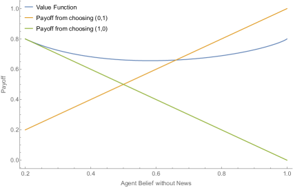
If the agent’s payoff from exerting effort until $\tau$ is just below the payoff from choosing the score $(0,1)$, then the moral hazard constraint binds, and the principal should set $r_{\tau,1}^{G}<1$. Note that a decrease in $r_{\tau,1}^{G}$ lowers both the payoff from stopping immediately, as well as the value function; however, the impact on the payoff from immediately stopping is larger since the prospect of obtaining $r_{\tau,0}^{N}(1-\mu_{\tau}^{N})$ following “no news” induces the agent to work, and this does not vary with $r_{\tau,1}^{G}$. So, if the moral hazard constraint is violated at time 0, then the principal should lower $r_{\tau,1}^{G}$ so that it binds.

So, consider how the scoring rule changes as $\mu_{0}^{N}$ (the initial belief that $\theta=1$) increases:

• For $\mu_{0}^{N}<c/\lambda_{1}^{G}$, it is impossible to induce the agent to acquire any information.

• There exists $\mu^{*}$ such that when $c/\lambda_{1}^{G}<\mu_{0}^{N}<\mu^{*}$, the optimal scoring rule involves $r_{\tau,1}^{G}=1$.

• There exists $\mu^{**}<1$ such that when $\mu^{*}<\mu_{0}^{N}<\mu^{**}$, the optimal scoring rule involves $r_{\tau,1}^{G}<1$, with the exact value pinned down by the condition that the agent is indifferent between (i) working continuously until their belief is $c/(\lambda_{1}^{G}r_{\tau,1}^{G})$ and (ii) never working at all.

• For $\mu_{0}^{N}>\mu^{**}$, it is impossible to induce the agent to acquire any information.

This observation clarifies why the principal may want to (but cannot) reoptimize the scoring rule. While giving the full reward from guessing state 1 is optimal if the agent initially assigns it probability less than $\mu^{*}$, for beliefs above this value, the reward from guessing state 1 must decrease. Now, even if the agent’s initial belief that $\theta=1$ is high, it will eventually decrease below $\mu^{*}$ with positive probability. On the other hand, offering the full reward when guessing state 1 after this time would defeat the initial purpose of starting with the lower reward—doing so would lead the agent to shirk and lie. In order to prevent this from happening, the principal must keep the initial reward low.

3.2 Stopping Strategies

We now show that one of the agent’s optimal strategies for exerting effort is a simple stopping strategy, simplifying the principal’s objective to maximization of the agent’s stopping time.

The agent can generally choose arbitrary, complex strategies for exerting effort. For example, the agent could wait for several periods before starting or randomize over such decisions. Nevertheless, we note that it is without loss for the agent to use a stopping strategy $\tau$—that is, slightly overloading the notation $\tau$ as a stopping time under a stopping strategy, we can assume that the agent chooses to exert effort at every time $t\leq\tau$, conditional on not having received any Poisson signal.

Lemma 1.

Given any contract $R$ and any best response of the agent with maximum effort length $z_{R}$ conditional on not receiving any Poisson signal, there exists a stopping strategy $\tau_{R}$ with $\tau_{R}\geq z_{R}$ that is also optimal for the agent.

Note that the maximum effort duration conditional on no Poisson signal arrival uniquely determines the information acquired by the agent. Moreover, whenever the agent works longer, the aggregated information acquired is Blackwell more informative, implying that the principal’s utility following the agent’s information acquisition is higher for any possible (principal) utility function. Therefore, Lemma 1 implies that the principal would seek to implement—and the agent would be willing to use—stopping strategies. Hence, it is without loss of generality to focus on them.

The proof for Lemma 1 is simple. Given any contract $R$ and any strategy of the agent (for instance, if the agent were potentially pausing effort for some time and resuming effort afterward), the agent does weakly better by front-loading effort to receive information earlier since this weakly increases his expected reward from the principal without increasing expected cost. Therefore, the resulting stopping strategy with the same effort length conditional on not receiving Poisson signals must also be optimal.

Principal’s objective

By restricting attention to stopping strategies, the principal’s payoff given any contract $R$ is uniquely determined by the stopping time $\tau_{R}$. Moreover, regardless of the principal’s valuation function $v$ for making decisions, the principal’s expected payoff is higher when $\tau_{R}$ is longer. As a result, the principal’s problem simplifies to designing a contract $R$ that maximizes the stopping time $\tau_{R}$ subject to the budget constraint. Under this objective, the design of the optimal contracts does not depend on the details of the principal’s valuation function $v$.

3.3 Menu Representation

As per the discussion in Section 3.2, we henceforth assume that the agent always chooses a stopping strategy for exerting effort. This observation further simplifies communication between the parties in the optimal contract. In particular, the agent need not report whether he has exerted effort in the current period. Instead, it is sufficient to incentivize the agent to truthfully report $s=G$ or $s=B$ immediately once observed, implicitly assuming that the agent indeed exerts effort in every period before the report.

We describe this menu representation for the dynamic contracts the principal might offer. The principal commits to a sequence of menu options at time $0$; at any time $t\leq T$, the agent can make a one-time, irrevocable choice from the set of available menus based on his posterior belief. Lemma 2 formalizes this menu representation.

Given any reward function $r:\Theta\to[0,1]$, let

$$u(\mu,r)\triangleq\text{\bf E}_{\theta\sim\mu}\!\left[{r(\theta)}\right]$$

be the agent’s expected utility given reward $r$ when his belief is $\mu$. In the binary state model (i.e., $\Theta=\{0,1\}$) we consider in this paper, we also represent the reward function as $r=(r_{0},r_{1})$, where $r_{0}$ is the reward for state being $0$ and $r_{1}$ is the reward for state being $1$.

Lemma 2 (menu representation).

Any dynamic contract $R$ implementing optimal stopping time $\tau_{R}$ is equivalent to a sequence of menu options $\{r^{s}_{t}\}_{t\leq\tau_{R},s\in S}\cup\{r^{N}_{\tau_{R}}\}$ where $r^{s}_{t}:\Theta\to[0,1]$. At any time $t\leq\tau_{R}$, the agent can make a one-time choice for the menu option $r^{*}$ from the subset $\mathcal{R}_{t}\triangleq\{r^{s}_{t^{\prime}}\}_{t\leq t^{\prime}\leq\tau_{R},s\in S}\cup\{r^{N}_{\tau_{R}}\}$, with the agent rewarded according to $r^{*}$ after time $T$. Moreover, at any time $t$, the utility of the agent with belief $\mu_{t}^{s}$ is maximized by picking the menu option $r^{s}_{t}$, i.e., for any $t\leq\tau_{R}$ and $s\in S$, or for $t=\tau_{R}$ and $s=N$,

$$u(\mu_{t}^{s},r_{t}^{s}) \geq u(\mu_{t}^{s},r),\quad\forall r\in\mathcal{R}_{t}.$$ (IC)

Section A.1 contains the proof of Lemma 2. Note that in Eq. IC, the agent’s incentives are uni-directional in time. That is, it is sufficient to consider the incentive constraints where the agent does not prefer to deviate from a truthful report when receiving an informative signal later.

Lemma 2 dramatically simplifies the space of contracts the principal needs to consider. For example, it allows us to convert the design of the optimal contracts into a sequence of linear programs such that the sequence of menu options in the optimal contract can be computed efficiently. We provide the details of the computational methods in Section A.2.

To simplify the exposition in later sections, given the menu representation in Lemma 2 for any contract $R$, for any time $t$ and any signal $s\in S$, we denote $u^{s}_{t}(R)\triangleq u(\mu_{t}^{s},r_{t}^{s})$ as the agent’s utility for not exerting effort in any time after $t$ when his current belief is $\mu_{t}^{s}$. We also omit $R$ from the notation when it is clear from the context. Moreover, for any $t<\tau_{R}$, we denote

$$r^{N}_{t}=\operatorname*{arg\,max}_{r\in\mathcal{R}_{t}}u(\mu_{t}^{N},r)$$

as the menu option the agent would choose at time $t$ if his belief were $\mu_{t}^{N}$. Let $u^{N}_{t}(R)\triangleq u(\mu_{t}^{N},r_{t}^{N})$.

3.4 An Auxiliary Static Model

To further illustrate the tensions in the dynamic model, we take a slight detour by considering an auxiliary static model with binary states $\Theta=\{0,1\}$ studied by Li et al., (2022). In Section 4, we will show how to connect this static model to our dynamic model and use this connection to prove the optimality of scoring rules in general dynamic environments. First, we review the characterizations of optimal scoring rules in the static model and their implications in this section.

Binary Effort Static Game

Consider an auxiliary static setting with binary effort. That is, the agent can choose to either not exert effort, leaving their prior belief unchanged, or exert effort and receive a signal $s\in\hat{S}$ according to signal structure $\sigma:\Theta\to\Delta(\hat{S})$ where the signal space $\hat{S}$ for the static setting is a measurable set. In the static model, the principal’s objective is to find a scoring rule that maximizes the expected difference in scores between exerting effort and not exerting effort, subject to a budget constraint on the scores. That is, letting $F$ be the distribution over posterior $\mu$ given the signal structure $\sigma$, the principal maximizes

$$\text{\bf E}_{\mu\sim F}\!\left[{\text{\bf E}_{\theta\sim\mu}\!\left[{P(\mu,\theta)}\right]}\right]-\text{\bf E}_{\theta\sim D}\!\left[{P(D,\theta)}\right]$$

subject to the constraint that $P(\mu,\theta)\in[0,1]$ for all $\mu\in\Delta(\Theta)$ and $\theta\in\Theta$. Intuitively, given any cost of exerting effort in the static model, the agent is more likely to be incentivized to exert effort when the score difference is larger. In the static model, call a scoring rule optimal if it provides the maximum score increase to the agent from exerting effort.

Optimal Scoring Rules

In the static model, it turns out that optimal scoring rules fall into the class of V-shaped scoring rules. A V-shaped scoring rule has an implementation whereby the agent guesses a state and obtains some reward amount (depending on the state), provided his guess is correct. The agent receives 0 if his guess is wrong.

Definition 2 (Li et al., , 2022).

A scoring rule $P$ is V-shaped with parameters $z_{0},z_{1}$ if

$$P(\mu,\theta)=\begin{cases}z_{1}&\mu\geq\frac{z_{0}}{z_{1}+z_{0}}\text{ and }\theta=1\\ z_{0}&\mu<\frac{z_{0}}{z_{1}+z_{0}}\text{ and }\theta=0\\ 0&\text{otherwise}.\end{cases}$$

We say $P$ is a V-shaped scoring rule with kink at $D$ if the parameters $z_{0},z_{1}$ satisfies $z_{0}=1,z_{1}=\frac{1-D}{D}$ if $D\geq\frac{1}{2}$ and $z_{0}=\frac{D}{1-D},z_{1}=1$ if $D<\frac{1}{2}$.

The terminology of the scoring rule as “V-shaped” comes from the property that the expected score $U_{P}(\mu)\triangleq\text{\bf E}_{\theta\sim\mu}\!\left[{P(\mu,\theta)}\right]$ is a V-shaped function. Furthermore, given any V-shaped scoring rule $P$ with kink at $D$, the agent with prior belief $D$ is indifferent between guessing the state is either 0 or 1.

Proposition 1 (Li et al., , 2022).

In the binary effort static game, for any prior $D$, a V-shaped scoring rule $P$ with kink at prior $D$ is optimal for all signal structures $\sigma$.

Proposition 1 provides an optimal solution for the static game. According to Li et al., , 2022, the V-shaped scoring rule $P$ is essentially the uniquely optimal scoring rule when the agent’s signals, received after exerting effort, are not fully revealing.

The underlying intuition for Proposition 1 is that in static environments, subject to the convexity constraint and the constraint that the expected score at the prior is a constant, V-shaped scoring rules maximize the expected score at all posteriors, thus providing the maximum incentives for the agent to exert effort. We emphasize that Proposition 1 implies that in the static model, the optimal scoring rule only depends on the prior $D$, not on the signal structure $\sigma$.

Proposition 1 illustrates one of the tensions in designing optimal contracts in dynamic environments. Ideally, the principal would want to design contracts that provide the optimal incentives for the agent to exert effort at any time $t\leq T$, since doing so would make them willing to work for the longest time possible. However, since the agent’s belief $\mu^{N}_{t}$ may drift over time, the scoring rules that provide the optimal incentives at time $t$ can be inconsistent with the scoring rules that are optimal for time $t^{\prime}$ when $t^{\prime}\neq t$. The dynamic incentives of the agent further imply that the optimal incentives cannot be achieved simultaneously at every time $t\leq T$. In Section 4, we will show that even with such tensions in the dynamic model, there are several canonical dynamic environments in which optimal contracts have an implementation as a scoring rule. We emphasize that this does not imply that the optimal scoring rules for the dynamic model necessarily coincide with the optimal scoring rules for the static model, and we will illustrate environments in which the optimal scoring rules for the dynamic model exhibit novel features in Sections 4.2 and 4.3.

4 Optimal Contracts as Scoring Rules

This section presents our main results on the implementation of the optimal contract as a static scoring rule in three canonical environments: stationary, perfect-learning and single-signal. Section 5 provides a partial converse to these results by showing that dynamic structures can be necessary to implement the optimal contract when all three conditions are violated. The main idea for the arguments in this section is to decompose the dynamic problem into multiple static problems. Specifically, we will consider a continuation game at any time $t$ where the agent only has two choices: To shirk forever or exert effort according to a specific strategy. Such continuation games essentially coincide with the static model introduced in Section 3.4. We will show that for any dynamic contract $R$, there exists a scoring rule $P$ that provides stronger incentives for the agent to exert effort in all continuation games, which further implies that the agent has stronger incentives to exert effort for a longer duration given scoring rule $P$ in the dynamic model. Appendix B contains the missing proofs in this section.

Continuation Game

For any time $0\leq t\leq t^{\prime}\leq T$, let $\mathcal{G}_{t,t^{\prime}}$ be the continuation game between $t$ and $t^{\prime}$. Specifically, the continuation game $\mathcal{G}_{t,t^{\prime}}$ is a static game with prior belief $\mu^{N}_{t-\Delta}$. Moreover, the agent has binary effort in the continuation game, i.e., the agent can choose either to (a) not exert effort or (b) follow the strategy of exerting effort until time $t^{\prime}$ (including time $t^{\prime}$) or a Poisson signal arrives. The cost of effort in this continuation game is $c\Delta$ times the expected number of periods the agent exerts effort between $t$ and $t^{\prime}$. Note that at any time $t$ in the dynamic environment, the agent has incentives to exert effort at time $t$ if there exists $t^{\prime}\geq t$ such that the agent has incentives to exert effort in the continuation game $\mathcal{G}_{t,t^{\prime}}$. For any contact $R$ with stopping time $\tau_{R}$, we say $\mathcal{G}_{t,\tau_{R}}$ is the continuation game at time $t$ for contract $R$. In the rest of the paper, we omit the subscript of $\tau_{R}$ from the notation when the contract $R$ is clear from context.

In the continuation game, for $t^{\prime}\geq t$, let $f^{s}_{t}(t^{\prime})$ be the probability mass function of receiving a Poisson signal $s$ at time $t^{\prime}$ conditional on not receiving Poisson signals before time $t$, and let $F^{s}_{t}(t^{\prime})$ be the corresponding cumulative distribution function. Given any contract $R$ with a sequence of menu options $\{r^{s}_{t}\}_{t\leq\tau_{R},s\in S}\cup\{r^{N}_{\tau_{R}}\}$, we refer to $u^{N}_{t-\Delta}(R)=u(\mu^{N}_{t-\Delta},r^{N}_{t-\Delta})$ as the no information payoff of the agent, and

$$U_{t}(R) \triangleq\left(1-\sum_{s\in S}F^{s}_{t}(\tau_{R})\right)\cdot u(\mu^{N}_{\tau_{R}},r^{N}_{\tau_{R}})+\sum_{t^{\prime}=t}^{\tau_{R}}\sum_{s\in S}u(\mu^{s}_{t^{\prime}},r^{s}_{t^{\prime}})\cdot f^{s}_{t}(t^{\prime})$$

as the continuation payoff of the agent in the continuation game $\mathcal{G}_{t}$. We also omit $R$ in the notations if it is clear from context. In the continuation game $\mathcal{G}_{t}$, the agent has incentives to exert effort if the payoff difference $U_{t}(R)-u^{N}_{t-\Delta}(R)$ is at least his cost of effort.

4.1 Stationary Model

The simplest case of interest is the stationary model, where the agent’s no information belief $\mu^{N}_{t}=D$ for all $t\leq T$. In this simple case, all continuation games at any time $t$ share the same prior belief. As illustrated in Proposition 1, the optimal scoring rules for all continuation games are the same. Therefore, the tension over time does not exist. In this case, it is straightforward to show that the optimal contract has an implementation as a V-shaped scoring rule with kink at the prior $D$, which is also the optimal scoring rule in the static model.

Theorem 1.

In the stationary model, an optimal contract can be implemented as a V-shaped scoring rule $P$ with kink prior $D$, for any prior $D$ and signal arrival rate.

4.2 Perfect-learning Environment

Outside of the stationary model, the no information belief $\mu^{N}_{t}$ of the agent drifts over time, meaning that the principal cannot provide optimal incentives to the agent in every continuation game. This section focuses on the perfect-learning environment where the agent fully learns the state upon receiving a Poisson signal. We show that the optimal contract has an implementation as a scoring rule for this environment. However, since the principal’s goal is to incentivize dynamic effort choices, the particular optimal scoring rule will differ from the optimal scoring rule in the static model.

Theorem 2.

An optimal contract $R$ exists with an implementation as a V-shaped scoring rule with parameters $r_{0}=1$ and $r_{1}\in[0,1]$ in the perfect-learning environment

Note that, unlike the stationary environment, although the optimal contract has an implementation as a static scoring rule, the kink of the scoring rule may not be at the prior $D$. In particular, the kink of the scoring rule depends on the parameter $r_{1}$, chosen to balance the agent’s incentive to exert effort at both time $0$ and the stopping time $\tau_{R}$. This observation illustrates the phenomenon that, despite the optimal contract having an implementation as a scoring rule, it does not coincide with the optimal scoring rule from the static model, and the dynamics in the effort choices still affect the design of optimal contracts.

Figure 2: The red lines are the agent’s utility $u^{N}_{t-\Delta}$ for not exerting effort, and the blue curve is the agent’s utility $U^{+}_{t}$ from exerting effort in at least one period, both as a function of the no information belief $\mu^{N}_{t-\Delta}$.

Next, we show how to identify the optimal parameter $r_{1}$ in the perfect-learning environment. We first ignore the constraint imposed by the time horizon $T$ momentarily. Given a V-shaped scoring rule $P$ with parameters $r_{0}=1$ and $r_{1}\in[0,1]$, recall that $u^{N}_{t}$ is the agent’s utility of from not exerting effort after time $t$. Let $U^{+}_{t}$ be the optimal utility of the agent, with respect to the prior belief $\mu^{N}_{t-\Delta}$, from exerting effort in at least one period starting from time $t$ (including $t$). By the Envelope Theorem, $U^{+}_{t}$ is convex in the no information belief $\mu^{N}_{t-\Delta}$ with its derivative between $-1$ and $r_{1}$. We let $\underline{\mu}(r_{1})=\bar{\mu}(r_{1})=2$ if $U^{+}_{t}<u^{N}_{t-\Delta}$ for all $t\geq 0$. Otherwise, let $\underline{\mu}(r_{1})=\min\{\mu^{N}_{t},t\geq 0:U^{+}_{t}\geq u^{N}_{t-\Delta}\}$ and $\bar{\mu}(r_{1})=\max\{\mu^{N}_{t},t\geq 0:U^{+}_{t}\geq u^{N}_{t-\Delta}\}$. The agent has incentives to exert effort at time $t$ given scoring rule $P$ if and only if $\mu^{N}_{t}\in[\underline{\mu}(r_{1}),\bar{\mu}(r_{1})]$. See Figure 2 for an illustration. In particular, the agent has incentives to exert effort at time $0$ if and only if $D\in[\underline{\mu}(r_{1}),\bar{\mu}(r_{1})]$.

Lemma 3.

Both $\underline{\mu}(r_{1})$ and $\bar{\mu}(r_{1})$ are weakly decreasing in $r_{1}$.

That is, by increasing the reward $r_{1}$ for prediction state 1 correctly in the scoring rule, the agent has incentives to exert effort for longer, i.e., $\underline{\mu}(r_{1})$ is smaller, but the agent has a weaker incentive to exert effort at time $0$, i.e., $\bar{\mu}(r_{1})$ is smaller. This tension illustrates an interesting dynamic effect in our model when the time horizon $T$ is sufficiently large. That is, there exist $\mu_{1}>\mu_{2}>\mu_{3}$ such that the agent can be incentivized to work when either the principal seeks to have the no information belief drift from (a) $\mu_{1}$ to $\mu_{2}$ or (b) $\mu_{2}$ to $\mu_{3}$, but not when seeking to have this belief drift from $\mu_{1}$ to $\mu_{3}$.

Let $\mu^{*}=\max_{r}\{\bar{\mu}(r):\bar{\mu}(r)\leq 1\}$. That is, $\mu^{*}$ is the maximum belief of the agent that can be incentivized to exert effort given any scoring rule. Thus, we can focus on the case where $D\leq\mu^{*}$. When there is a time horizon constraint $T$ for exerting effort, let $r_{T}=1$ if $\underline{\mu}(1)>\mu^{N}_{T}$ and let $r_{T}\in[0,1]$ be the minimum parameter such that $\underline{\mu}(r_{T})=\mu^{N}_{T}$ otherwise.

Proposition 2.

In the perfect-learning environment, no contract incentivizes the agent to exert effort if $D>\mu^{*}$ or $D<\underline{\mu}(1)$. Otherwise, the optimal parameter $r_{1}$ in a V-shaped scoring rule is the maximum value below $r_{T}$ such that $\bar{\mu}(r_{1})\geq D$.

Intuitively, the optimal parameter $r_{1}$ maximizes the stopping time subject to the constraint that the agent has incentives to exert effort at time $0$.

We illustrate the ideas behind the proof of Theorem 2. We first show that in perfect-learning environments, it is without loss of optimality to consider contracts where the menu options provide a maximum reward to the agent for receiving a bad news signal or no Poisson signal at all when the state is $0$. Recall that $0$ is the state that the agent’s posterior belief drifts to absent a Poisson signal.

Lemma 4.

In the perfect-learning environment, for any prior $D$ and any signal arrival probabilities $\lambda$, there exists an optimal contract $R$ with a sequence of menu options $\{r^{s}_{t}\}_{t\leq\tau_{R},s\in S}\cup\{r^{N}_{\tau_{R}}\}$ such that $r^{B}_{t}=r^{N}_{\tau_{R}}=(1,0)$ for any $t\leq\tau_{R}$.

Intuitively, for any contract $R$ with stopping time $\tau_{R}$, we consider another dynamic contract $\bar{R}$ that rewards the agent the maximum amount of $1$ following state $0$ conditional on the event that the agent receives a bad news signal at any time before $\tau_{R}$ or no Poisson signal until time $\tau_{R}$. In the perfect-learning environment, such an event occurs with probability 1 if the state is $0$. Therefore, whenever the state is $0$, the agent enjoys the full increase in rewards in any continuation game $\mathcal{G}_{t}$ for exerting effort. By contrast, the increase in the expected reward when not exerting effort in the continuation game $\mathcal{G}_{t}$ is at most the prior probability of state $0$ times the reward increase. Thus, the agent has stronger incentives to exert effort in all continuation games given contract $\bar{R}$, which implies that contract $\bar{R}$ must also be optimal in the dynamic model.

Next, we show that offering a single menu option for rewarding good news signals is also sufficient. Intuitively, the dynamic incentives of the agent imply that in any contract $R$, the agent’s reward for receiving a good news signal must decline over time. We show that by decreasing earlier rewards to make the agent’s utility from early stopping sufficiently low and increasing later rewards to make the reward from continuing effort sufficiently high, the resulting contract has an implementation as a scoring rule, and the agent’s incentive for exerting effort increases weakly in all continuation games given the new contract. This idea is illustrated formally in the following proof.

Proof of Theorem 2.

By Lemma 4, it is without loss of optimality to focus on contract $R$ with a sequence of menu options $\{r^{s}_{t}\}_{t\leq\tau_{R},s\in S}\cup\{r^{N}_{\tau_{R}}\}$ such that $r^{B}_{t}=r^{N}_{\tau_{R}}=(1,0)$ for any $t\leq\tau_{R}$. In addition, since signals are perfectly revealing, it is without loss to assume that $r^{G}_{t,0}=0$ and the incentive constraints imply that $r^{G}_{t,1}$ is weakly decreasing in $t$.

Let $\hat{t}\in[0,\tau_{R}]$ be the maximum time such that an agent with no information belief $\mu^{N}_{\hat{t}}$ weakly prefers menu option $r^{G}_{\hat{t}}$ compared to $r^{N}_{\tau_{R}}$. Since both $\mu^{N}_{t}$ and $r^{G}_{t,1}$ are weakly decreasing in $t$, an agent with posterior belief $\mu^{N}_{t}$ weakly prefers $r^{G}_{t^{\prime}}$ compared to $r^{N}_{\tau_{R}}$ for any $t,t^{\prime}\leq\hat{t}$, and weakly prefers $r^{N}_{\tau_{R}}$ compared to $r^{G}_{t^{\prime}}$ for any $t,t^{\prime}>\hat{t}$. Now consider another contract $\hat{R}$ that offers only two menu options, $r^{G}_{\hat{t}}$ and $r^{N}_{\tau_{R}}$, at every time $t\leq\tau_{R}$. Contract $\hat{R}$ can be implemented as a V-shaped scoring rule with parameters $r_{0}=1$ and $r_{1}=r^{G}_{\hat{t},1}\in[0,1]$. Moreover, at any time $t\leq\tau_{R}$,

• if $t>\hat{t}+\Delta$, in the continuation game $\mathcal{G}_{t,\tau_{R}}$, the agent’s utility for not exerting effort is the same in both contract $R$ and $\hat{R}$ because the agent with no information belief $\mu^{N}_{t-\Delta}$ will choose the same menu option $r^{N}_{\tau_{R}}$. However, the agent’s utility for exerting effort is weakly higher in contract $\hat{R}$ since the reward $r^{G}_{t,1}$ from receiving a good news signal at time $t$ weakly decreases in $t$.

• if $t\leq\hat{t}+\Delta$, in the continuation game $\mathcal{G}_{t,\tau_{R}}$, by changing the contract from $R$ to $\hat{R}$, the decrease in agent’s utility for not exerting effort is exactly $\mu^{N}_{t-\Delta}(r^{G}_{t-\Delta,1}-r^{G}_{\hat{t},1})$ by changing the optimal menu option for no information belief $\mu^{N}_{t-\Delta}$ from $r^{G}_{t-\Delta}$ to $r^{G}_{\hat{t}}$. However, the decrease in the agent’s utility for exerting effort in $\mathcal{G}_{t,\tau_{R}}$ is at most $\mu^{N}_{t-\Delta}(r^{G}_{t-\Delta,1}-r^{G}_{\hat{t},1})$ since the decrease in reward for receiving a good news signal $G$ is at most $r^{G}_{t-\Delta,1}-r^{G}_{\hat{t},1}$ and it only occurs when the state is $1$.

Therefore, given contract $\hat{R}$, the agent has stronger incentives to exert effort in all continuation games $\mathcal{G}_{t,\tau_{R}}$ with $t\leq\tau_{R}$, which implies that $\tau_{\hat{R}}\geq\tau_{R}$ and hence contract $\hat{R}$ is also optimal. ∎

4.3 Single-signal Environment

In this section, we consider the single-signal environment where the agent’s belief drifts towards $0$ in the absence of a Poisson signal and jumps towards $1$ when a Poisson signal arrives. In the single-signal environment, we do not assume that the signals are fully revealing.

Theorem 3.

An optimal contract with an implementation as a scoring rule exists in the single-signal environment.

Note that in the single-signal environment, although the optimal contract can be implemented as a static scoring rule, it may not be implementable as a V-shaped scoring rule when the signals are not fully revealing. Put differently, the principal may not want to simply let the agent guess the state and reward the agent only following a correct guess. By contrast, the principal may benefit from rewarding the agent even when the guess is wrong.

Figure 3: The red lines are the agent’s utility $u^{N}_{t-\Delta}$ for not exerting effort, and the blue curve is the agent’s utility $U^{+}_{t}$ from exerting effort in at least one period, both as a function of the no information belief $\mu^{N}_{t-\Delta}$. The black curve is the agent’s utility for not exerting effort in the alternative scoring rule with additional menu option $(z_{0},z_{1})$.

Consider an interpretation of the minimum reward across the two states as the “base reward” and the difference between the rewards as the “bonus reward.” From this perspective, our results indicate that it may be necessary to consider scoring rules where the base reward is strictly positive. This observation may seem counterintuitive, as providing a strictly positive base reward strictly decreases the maximum bonus reward for the agent due to the budget constraint. In principle, providing a positive base reward should lower the agent’s utility increase when correctly guessing the state and, hence, subsequently lower the agent’s incentive for exerting effort.

The correct intuition is as follows: providing a strictly positive base reward to the agent at time $t$ only decreases the agent’s incentive to exert effort at time $t$; however, it increases the agent’s incentive to exert effort at earlier times $t^{\prime}<t$ since the agent may expect high rewards for exerting effort, even though he might make mistakes in guessing the states after receiving (imperfectly informative) Poisson signals. This modification benefits the principal if the agent’s incentive constraint for exerting effort initially binds at time 0, but becomes slack at intermediate time $t\in(0,\tau_{R})$. As illustrated in Figure 3 and in Section 4.2, by implementing the optimal V-shaped scoring rule, the agent’s incentive for exerting effort is binding only at the extreme time $0$ with belief $D=\bar{\mu}(r_{1})$ and time $\tau_{R}$ with belief $\mu^{N}_{\tau_{R}}=\underline{\mu}(r_{1})$. In this case, since the signals are not perfectly revealing, there may exist a time $t$ such that $\mu^{G}_{t}<D$. By providing an additional menu option with strictly positive base reward in the scoring rule to increase the agent’s utility at beliefs $\mu^{G}_{t}$ (e.g., the additional menu option $(z_{0},z_{1})$ illustrated in Figure 3), the agent’s incentive constraint for exerting effort at time $0$ is relaxed and the contract thus provides the agent incentives to exert effort following more extreme prior beliefs without influencing the stopping belief $\underline{\mu}(r_{1})$.

We illustrate the main ideas for Theorem 3. Note that given any (static) scoring rule, the utility $u^{N}_{t}$ of the agent from not exerting effort is a convex function of his no information belief $\mu^{N}_{t}$ (see Lemma 8). Therefore, to show that the optimal contract can be implemented as a scoring rule, we first show that it is without loss to focus on dynamic contracts where the $u^{N}_{t}$ is convex in $\mu^{N}_{t}$.

Lemma 5.

In the single-signal environment, an optimal contract exists with the no-information utility $u^{N}_{t}$ convex in $\mu^{N}_{t}$.

Intuitively, in the optimal contract, if the no-information utility is not convex, one of the following cases holds at time $\bar{t}$, the earliest time such that the utility is non-convex:

• the agent’s incentive for exerting effort is slack at time $\bar{t}+\Delta$. In this case, we can increase the no-information utility at time $\bar{t}$ by increasing the rewards in menu option $r^{N}_{t}$ such that either (a) the incentive for exerting effort at time $\bar{t}+\Delta$ will bind, or (b) the no-information utility will become convex at $\bar{t}$.

• the agent’s incentive for exerting effort is slack at time $\bar{t}+\Delta$. In this case, the combination of the no-information utility function’s non-convexity and the contract’s incentive constraint actually implies that the agent will have a strict incentive to stop exerting effort at time $\bar{t}$. See Figure 6 in Section B.3 for an illustration.

Note that although the convexity in no-information utility function implies that the optimal contract has an implementation as a scoring rule, it does not necessarily imply that the resulting scoring rule must satisfy the ex-post budget constraint or the ex-post individual rationality constraint. For example, consider a convex no-information utility function $u^{N}_{t}=(\mu^{N}_{t})^{2}$. A simple dynamic contract that implements this no-information utility function is to offer a constant reward $(\mu^{N}_{t})^{2}$ at time $t$ regardless of the realization of the state. However, if the principal wants to implement this utility function using a static scoring rule, by Lemma 8, the menu option for belief $\mu\in[0,1]$ must be $(-\mu^{2},2\mu-\mu^{2})$, which violates the ex post individual rationality constraint.

Figure 4: The black curve is the convex no-information utility of the agent, and $\hat{t}$ is the minimum time with a bounded tangent line (red line). The thick dashed line is the no-information utility of the agent given a feasible scoring rule that offers a menu option that corresponds to the red line instead of the black curve for belief $\mu\geq\mu^{N}_{t}$.

Primarily, a violation of the ex-post budget constraint or the individual rationality constraint emerges because the no-information utility function is too convex. In this case, we can flatten the no-information utility by decreasing the reward to the agent at earlier times. We can show that by flattening the no-information utility, the decrease in no-information utility is weakly larger than the decrease in continuation payoff in all continuation games, and hence, the agent has stronger incentives to exert effort. Figure 4 illustrates this idea, with details provided in Section B.3.

5 Optimality of Dynamic Contracts

This section shows that the optimal scoring rule must be dynamic when (i) signals are noisy and (ii) the drift is sufficiently slow. More precisely, we consider cases where both good and bad news signals can arrive with strictly positive probability if the agent exerts effort. That is, we have $\lambda_{1}^{G}>\lambda_{0}^{G}>0$ and $0<\lambda_{1}^{B}<\lambda_{0}^{B}$. Recall that we have assumed that $\lambda_{1}^{G}+\lambda_{1}^{B}>\lambda_{0}^{G}+\lambda_{0}^{B}$, meaning that “no news is bad news.” Taking the drift to be slow means that the above difference is small. Signals being noisy means that they do not reveal the state.

Let $\mu_{\lambda,c}\triangleq\min\{\frac{1}{2},\frac{c}{\lambda^{G}_{1}-\lambda^{G}_{0}}\}$ and let $T_{\lambda,D,c}$ be the maximum time such that $\mu^{N}_{T_{\lambda,D,c}-\Delta}\geq\mu_{\lambda,c}$. Intuitively, $T_{\lambda,D,c}$ is the maximum calendar time such that the agent can be incentivized to exert effort in any contract when the prior is $D$.

Lemma 6.

The stopping time $\tau_{R}$ satisfies $\tau_{R}\leq T_{\lambda,D,c}$, given any prior $D\in(0,1)$, arrival rates $\lambda$, cost of effort $c$, and contract $R$ that satisfies the budget constraint.

Appendix C contains this section’s missing proofs.

Theorem 4.

Given any prior $D\in(0,\frac{1}{2})$, any cost of effort $c$, and any constant $\kappa_{0}>0,\frac{1}{4\Delta}\geq\bar{\kappa}_{1}>\underline{\kappa}_{1}>0$, there exists $\epsilon>0$ such that for any $T\geq T_{\lambda,D,c}$ and $\lambda$ satisfying

• $\lambda^{G}_{1}-\lambda^{G}_{0}\geq\frac{1}{D}(c+\kappa_{0})$; (sufficient-incentive)

• $\lambda_{1}^{B},\lambda_{0}^{B},\lambda_{0}^{G},\lambda_{1}^{G}\in[\underline{\kappa}_{1},\bar{\kappa}_{1}]$; (noisy-signal)

• $\lambda_{1}^{G}+\lambda_{1}^{B}\in(\lambda_{0}^{G}+\lambda_{0}^{B},\lambda_{0}^{G}+\lambda_{0}^{B}+\epsilon)$, (slow-drift)

any static scoring rule is strictly suboptimal.

Theorem 4 provides sufficient conditions that necessitate the use of complex dynamic structures in the optimal contract to incentivize dynamic effort. The condition that $T\geq T_{\lambda,D,c}$ implies that the time horizon $T$ will not be a binding constraint for the agent to exert effort. The sufficient incentive condition avoids trivial solutions by ensuring that the cost of effort $c$ is sufficiently small compared to the difference in arrival rates of the good news signal, so that the agent has incentives to exert effort for a strictly positive length of time in the optimal contract. The noisy-signal condition rules out the perfect-learning environment and the single-signal environment, and the slow-drift condition rules out the stationary environment. Moreover, the single-signal environment can also be viewed as the extreme opposite of the slow-drift condition, since the difference in arrival rates of the signals is maximal and the belief drifts to 0 quickly in the absence of a Poisson arrival.

A substantial assumption that appears harmless is that $D\in(0,\frac{1}{2})$. Note that combining this with our restriction to environments where the belief absent a Poisson signal drifts towards 0, our theorem only applies to environments where the agent’s posterior belief absent a Poisson signal becomes more polarized towards the more likely states given the prior belief. This restriction ensures that the following myopic-incentive contract we define is incentive compatible for the agent.

Definition 3.

When prior $D\in(0,\frac{1}{2})$, a contract $R$ with menu options $\{r^{s}_{t}\}_{t\leq\tau_{R},s\in S}\cup\{r^{N}_{\tau_{R}}\}$ is a myopic-incentive contract if $r^{N}_{\tau_{R}}=r^{G}_{t}=(1,0)$ and $r^{B}_{t}=(\frac{\mu^{N}_{t}}{1-\mu^{N}_{t}},0)$ for any $t\geq 0$.

Figure 5: Illustration of myopic-incentive contract. The solid line is the expected reward of the agent, as a function of his belief, for not exerting effort and reporting his belief truthfully at time $t$.

Intuitively, the sequence of menu options offered by the myopic-incentive contract is such that at any time $t$, the agent with belief $\mu^{N}_{t}$ is indifferent between all menu options offered at time $t$. See Figure 5 for an illustration. The condition that the belief absent a Poisson signal becomes increasingly polarized implies that the rewards in menu options decrease over time. This property is necessary for the constructed contract to be incentive-compatible for the agent.

Note that the construction of menu options in the myopic-incentive contract at any time $t$ resembles the V-shaped scoring rules that are optimal for the static model with prior $\mu^{N}_{t}$. However, the myopic-incentive contract does not provide the optimal incentive for the agent to exert effort in all continuation games. This observation holds because, in the continuation game $\mathcal{G}_{t}$, the agent may receive a Poisson signal after time $t$, when the reward for reporting the received signal decreases. Thus, the myopic-incentive contract may not always be optimal for the principal. Nonetheless, we show that when the drift of belief is sufficiently slow, the myopic-incentive contract provides incentives close to the optimal contract.

Lemma 7.

Given any prior $D\in(0,\frac{1}{2})$, any cost of effort $c$, any constant $\underline{\kappa}_{1}>0$, and any $\eta>0$, there exists $\epsilon>0$ such that for any $T\geq T_{\lambda,D,c}$ and any $\lambda$ satisfying that $\lambda^{s}_{\theta}\leq\frac{1}{4\Delta}$ for all $s\in S$ and $\theta\in\{0,1\}$, and

• $\lambda^{G}_{1}-\lambda^{G}_{0}\geq\frac{1}{D}(c+\kappa_{0})$; (sufficient-incentive)

• $\lambda_{1}^{G}+\lambda_{1}^{B}\leq\lambda_{0}^{G}+\lambda_{0}^{B}+\epsilon$, (slow-drift)

letting $R$ be the myopic-incentive contract (Definition 3), we have $\mu^{N}_{\tau_{R}}-\mu^{N}_{T_{\lambda,D,c}}\leq\eta$.

When the drift of no information belief is sufficiently slow compared to the arrival rates of the Poisson signals, with sufficiently high probability, the agent will receive a Poisson signal before the no information belief drifts far away from his initial belief. In this case, the decrease in rewards over time in the myopic-incentive contract does not significantly weaken the agent’s incentive for exerting effort. Hence, the myopic-incentive contract is approximately optimal for the principal.

By contrast, if the principal instead uses a contract that can be implemented as a scoring rule, given stopping time $\tau_{R^{*}}$ in the optimal contract $R^{*}$, this scoring rule must be close to the optimal scoring rule in the continuation game $\mathcal{G}_{t}$ for any $t$ that is sufficiently close to $\tau_{R^{*}}$ in order to incentivize the agent to exert effort in continuation game $\mathcal{G}_{t}$. However, when the signals are noisy, as illustrated in Section A.4, such scoring rules fail to provide sufficient incentives for the agent to exert effort at time $0$, leading to a contradiction. Intuitively,the myopic-incentive contract avoids this conflict in incentives by providing higher rewards to the agent upon receiving a bad new signal $B$ without affecting the agent’s incentive to report the acquired information truthfully. In particular, higher rewards upon Poisson signal arrivals strengthen the agent’s incentives to exert effort at any time $t$.

General characterizations

In Lemma 7, we construct the myopic-incentive contract that is approximately optimal when the drift is slow and the belief absent a Poisson signal is polarizing. Although the stated contract is generally not fully optimal, a similar decreasing reward structure does, in fact, characterize the principal’s exact optimum.

To simplify notation, first recall that any menu option $r$ has a representation as a tuple $(r_{0},r_{1})$. For any pair of menu options $r,r^{\prime}$, we define $r^{\prime}\preceq r$ if $r^{\prime}_{0}\leq r_{0}$ and $r^{\prime}_{1}\leq r_{1}$. That is, $r^{\prime}\preceq r$ if $r^{\prime}$ is at most $r$ in all components.

Theorem 5.

For any prior $D$ and any signal arrival rates $\lambda$, there exists an optimal contract $R$ with optimal stopping time $\tau_{R}$ and a sequence of menu options $\{r^{s}_{t}\}_{t\leq\tau_{R},s\in S}\cup\{r^{N}_{\tau_{R}}\}$ such that (1) $r^{N}_{\tau_{R}}=r^{B}_{\tau_{R}}$; (2) $r^{B}_{t^{\prime}}\preceq r^{B}_{t}$ for all $t^{\prime}\geq t$; (3) $r^{B}_{t,0}=1$ if $r^{B}_{t,1}>0$; and (4) for any $t\leq\tau_{R}$,

$$r^{G}_{t}=\operatorname*{arg\,max}_{r:\Theta\to[0,1]} \ u(\mu_{t}^{s},r)$$

s.t. $$\ u(\mu_{t^{\prime}}^{N},r_{t^{\prime}}^{B})\geq u(\mu_{t^{\prime}}^{N},r),\quad\forall t^{\prime}\in[0,t].$$

Compared to the menu representation in Lemma 2, the simplification in Theorem 5 is the optimality of providing a decreasing sequence of rewards when receiving a bad news signal $B$ in both states. Additionally, the optimal sequence of rewards for signal $B$ satisfies the condition that the contract initially maintains the maximum score for state $0$ and reduces the reward for state $1$. This phase is followed by a decrease in the reward for state $0$, maintaining the minimum score for state $1$. Recall that state $0$ represents the state toward which the agent’s belief drifts absent a Poisson signal. Furthermore, the sequence of rewards following bad news signals uniquely determines the optimal contracts. In other words, given the rewards for receiving bad news signals, the rewards for receiving good news signals $G$ maximize the agent’s utility while ensuring that the agent with belief $\mu^{N}_{t}$ weakly prefers the menu option for signal $B$ over $G$ for all times $t$.

However, it is worth noting that Theorem 5 does not specify the rate of reward decrease in the optimal contract, which depends on the primitives of the model. While the optimal sequence of rewards can be efficiently computed through linear programming (for details, refer to Section A.2), it may not have simple closed-form characterizations. Despite the challenges of deriving closed-form characterizations, our results in Section 4 still show that maintaining constant rewards over time is optimal in several canonical environments.

6 Extensions and Discussions

We now turn to some extensions of the main model, particularly those related to randomized contracts, non-stationary information acquisition, and ex-ante budget constraints. We show how to generalize our results and techniques to such environments. Finally, we conclude our paper and propose several open questions in Section 6.4.

6.1 Randomized Contracts

Although deterministic contracts are appealing for practical applications, in some cases, a principal could commit to randomized contracts with the help of a public randomization device. To speak to this possibility, let $\varsigma=\left\{\varsigma_{t}\right\}_{t\leq T}$ be a sequence of random variables with $\varsigma_{t}$ drawn from a uniform distribution in $[0,1]$. A randomized contract is a mapping

$$R(\cdot|\varsigma):\mathcal{H}_{T}\times\Theta\to[0,1].$$

Crucially, in randomized contracts, at any time $t$, the history of the randomization device $\left\{\varsigma_{t^{\prime}}\right\}_{t^{\prime}\leq t}$ is publicly revealed to the agent before determining his choice of effort or the message sent to the principal. The randomization revealed before $t$ affects the agent’s incentives after time $t$, and without it, such contracts reduce back to deterministic contracts.

Given randomized contracts, the agent’s optimal strategy need not be a simple stopping strategy. In particular, the agent may decide whether to work or not depending on the public randomization’s past realizations. The agent may also strategically delay exerting effort to wait for the realization of the public randomization. As a result, the simplified objective of maximizing the stopping time of the agent is not appropriate for randomized contracts, and we need to consider the original objective of maximizing expected payoff $\text{\bf E}\!\left[{v(a,\theta)}\right]$ subject to the budget constraint.

When randomized contracts are allowed, principal objective functions could exist under which randomized contracts are beneficial. The main intuition is that at some time $t$, the principal can randomly inflate or decrease the rewards of the agent in the menu options, setting the probability of a decrease to be much larger to preserve the agent’s dynamic incentives for truthful reporting. Then, after time $t$, with a small probability, rewards inflate, and the agent has incentives to exert effort for longer without a Poisson signal arrival— i.e., the realized stopping time increases. Such a modification is beneficial if the principal only values extreme posterior beliefs.

To illustrate this intuition more formally, consider an environment where learning is perfect and only good news signal $G$ arrives with positive probability. By Theorem 2, under deterministic contracts, a V-shaped scoring rule with parameters $r_{0}=1$ and $r_{1}\in[0,1]$ implements the optimal contract $R$. Moreover, when the time horizon $T$ is sufficiently large, $r_{1}$ is chosen such that the agent with prior belief $D$ is indifferent between exerting effort or not, and it is easy to construct instances where $r_{1}<1$. Let $\tau_{R}$ be the stopping time in the optimal deterministic contract, and let $\mu^{N}_{\tau_{R}}$ be the stopping belief when the agent never receives any Poisson signals.

Now, suppose the principal faces a binary decision to make at time $T$. That is, $A=\{0,1\}$. The payoff of the principal is $v(0,\theta)=0$ for all $\theta\in\Theta$, and $v(1,0)=1,v(1,1)=-\frac{1-\mu^{N}_{\tau_{R}}}{\mu^{N}_{\tau_{R}}}$; plainly, the principal only seeks to change her action from 1 to 0 if the posterior belief is below $\mu^{N}_{\tau_{R}}$. In this case, the principal’s benefit from acquiring information from the agent using a deterministic contract is 0. However, the following argument shows that the principal’s payoff from a randomized contract can be strictly positive. Let $\delta\in(0,1-r_{1}]$ be the maximum number such that (1) the agent has strict incentives to exert effort until time $\frac{2\tau_{R}}{3}$ in the absence of a Poisson signal given menu options $(1,0)$ and $(0,r_{1}-\delta)$; and (2) the agent can be incentivized to exert effort given menu options $(1,0)$ and $(0,r_{1}+\delta)$ when the prior belief is $\mu^{N}_{\frac{\tau_{R}}{2}}$. Now consider the randomized contract $\hat{R}$ that provides menu options $(1,0)$ and $(0,r_{1}-\delta)$ from time $0$ to $\frac{\tau_{R}}{2}$, and after time $\frac{\tau_{R}}{2}$, the principal offers menu options $(1,0)$ and $(0,r_{1}+\delta)$ with probability $\epsilon^{2}$, offers menu options $(1,0)$ and $(0,0)$ with probability $\epsilon$, and offers the same menu options $(1,0)$ and $(0,r_{1}-\delta)$ with the rest probabilities. It is easy to verify that with sufficiently small $\epsilon>0$, the agent still incentives to exert effort at any time $t\leq\frac{\tau_{R}}{2}$. Moreover, after time $\frac{\tau_{R}}{2}$, with probability $\epsilon^{2}$, the realized menu options are $(1,0)$ and $(0,r_{1}+\delta)$, and the agent can be incentivized to exert effort to a time strictly larger than $\tau_{R}$ in the absence of a Poisson signal. Therefore, randomized contract $\hat{R}$ provides a strictly positive payoff to the principal, outperforming all deterministic contracts.

6.2 Non-stationary Environments

Our model assumes that the cost of acquiring information is fixed over time, as is the mapping from states into signals when the agent exerts effort. On the other hand, many of our techniques and results do not rely on these assumptions, particularly as we focus on maximizing the incentive for the agent to exert effort. Our results extend unchanged if the cost of exerting effort is $c(\tilde{t})\Delta$, whenever the agent has exerted effort for $\tilde{t}$ units of time and $c(\cdot)$ is a non-decreasing function. In this case, the agent’s strategy again without loss is a stopping time, and identical arguments imply that scoring rules maximize the incentive to exert effort under any of the three environments discussed.

We can similarly allow for time dependence in the informational environment. Specifically, we can allow for the arrival rates of signals at any time to depend on the amount of effort the agent has exerted until that point. That is, suppose that if the agent has exerted effort for $\tilde{t}$ units of time, then exerting effort produces a good news signal arrives in state $\theta$ with probability $\lambda_{\theta,\tilde{t}}^{G}\Delta$, and a bad news signal with probability $\lambda_{\theta,\tilde{t}}^{B}\Delta$ (and no signal with complementary probability). While seemingly minor, this modification induces more richness in the set of possible terminal beliefs as a function of the effort history—for instance, if the terminal beliefs are always in the set $\{\underline{p},\overline{p}\}$, despite drifting over time.

Our proof techniques did not make use of the particular belief paths induced by constant arrival rates and hence extend to this case, with the minor exception that Theorem 3 requires $\mu_{t}^{G}$ to be weakly monotone as a function of time (a property that holds when the arrival rate is constant). Otherwise, as long as parameters stay within each environment articulated in Section 4, the proofs of these results extend unchanged.

6.3 Ex Ante Budget Constraints

In this paper, we require the principal’s budget constraint to be satisfied ex-post, and a natural extension is to relax it by considering ex-ante budget constraints. Note that in our model, we still need to impose limited liability on the agent—in other words, the reward should satisfy $r\geq 0$ ex-post. Suppose the ex-ante individual rationality constraint replaces the ex-post limited liability constraint. In that case, there is no constraint on the rewards for off-path behaviors of the agent. Hence, the principal can easily implement the first best, where the agent’s total cost of effort equals the ex-ante budget, by designing contracts that punish the agent for deviation. Therefore, we focus on the model with ex-ante budget constraints and ex-post limited liability constraints.

We show that in the special case where the conditions in both perfect-learning environments and single-signal environments are satisfied, i.e., when $\lambda^{B}_{0}=\lambda^{B}_{1}=\lambda^{G}_{0}=0$ and only $\lambda^{G}_{1}>0$, the optimal contract can also be implemented as a scoring rule. Section D.1 contains details for this claim. This observation illustrates that the optimality of static contracts extends under ex-ante budget constraints under natural assumptions. We conjecture that our result also extends when only conditions in one of the environments are satisfied, although the formal arguments for this conjecture may require additional novel ideas.

By relaxing the ex-post budget constraints, we can also apply our results to models where the principal values the rewards for the agent. In particular, when the principal values the rewards, the problem can be decoupled into two orthogonal problems: (1) maximizing the expected payoff from the decision problem subject to the ex-ante budget constraints and (2) optimizing the budgets to maximize the expected utility of the principal. Our results under ex-ante budget constraints imply that even when the principal values the rewards, the optimal contract can still be implemented as a scoring rule when only $\lambda^{G}_{1}>0$.

6.4 Conclusions

This paper has introduced a framework to consider optimal scoring rule design when the agent faces an information acquisition problem that is fundamentally dynamic. Indeed, natural stories for why information acquisition is costly involve some dynamic element—for instance, a student deciding how long to work on coming up with a proof or counterexample or researchers deciding how long to run tests to learn about a drug’s efficacy. Our assumptions on information arrival are inspired by and generalized those from past work on dynamic endogenous information acquisition; however, a fundamental difficulty in our problem was the lack of any natural structure, such as stationarity, given arbitrary dynamic contracts. Such assumptions are often critical in similar exercises. Nevertheless, we provided simple conditions such that the optimal dynamic contract is implementable by a scoring rule and explained the extent to which these conditions are necessary for this conclusion to hold.

There are many natural avenues for future work. For instance, since our goal was to optimize among dynamic contracts in a setting with dynamic moral hazard, we have neglected information arrival processes as general as those accommodated by Chambers and Lambert, (2021)—for instance, if the information the agent acquires over time relates to what information will arrive in the future. While we found the analysis under the particular class of information arrival processes considered tractable, we do not doubt that similar conclusions could emerge under different information arrival processes. Finding a richer class of tractable information arrival processes would also be necessary to allow for more of an intensive margin for experimentation relative to what we have allowed. In these cases, scoring rules may not be a natural class to consider, leading to the natural follow-up question of whether there are other simple ways of understanding how the principal may optimally leverage the dynamic nature of the problem.

Conversely, one may also be interested in these cases whether scoring rules incur significant loss relative to optimal dynamic contracts. Our goal here has been to provide a framework to study optimal contracts in dynamic settings, and we find further insights on this agenda valuable.

Appendix A Additional Preliminaries

A.1 Menu Representation

Proof of Lemma 2.

By the revelation principle, it is without loss to focus on contracts where the agent truthfully reports whether he exerts effort or not and the received signal at each time $t$. That is, the message space at any time $t$ is $\{0,1\}\times\{G,B,N\}$ where $1$ represents exerting effort and $0$ represents not exerting effort.

Next we construct the sequence of menu options $\{r^{s}_{t}\}_{t\leq\tau_{R},s\in S}\cup\{r^{N}_{\tau_{R}}\}$ that corresponds to a contract $R$ that induces truth-telling. Let $\tau_{R}$ be the stopping time of contract $R$. For any time $t\leq\tau_{R}$, for any signal $s\in S$, let $h^{s}_{t}$ be the history of reports the agent sends if he receives signal $s$ at time $t$. That is, in history $h^{s}_{t}$, the agent sends $(1,N)$ before time $t$, $(1,s)$ at time $t$, and $(0,N)$ after time $t$. Let $h^{N}_{\tau_{R}}$ be the history of reports the agent sends if he didn’t receive any Poisson signal at all.

For any time $t\leq\tau_{R}$ and any signal $s\in S$, let $r^{s}_{t}=R(h^{s}_{t},\cdot)$ and let $r^{N}_{\tau_{R}}=R(h^{N}_{\tau_{R}},\cdot)$. Given this constructed sequence of menu options, the incentive constraints in Eq. IC is satisfied since contract $R$ induces truth-telling. Moreover, it is easy to verify that the agent’s utility for stopping effort at any time $t\leq\tau_{R}$ is the same given both the menu representation and the original contract $R$. Therefore, the stopping time of the agent given this menu representation is also $\tau_{R}$. ∎

A.2 Efficient Algorithms for Computing Optimal Contracts

Let $\tau\leq T$ be the stopping time in the optimal contract. We know that there exists a contract $R$ such that the agent has incentive to exert effort in all continuation $\mathcal{G}_{t,\tau}$ with $t\leq\tau$. Therefore, to compute the optimal contract, it is sufficient to enumerate all stopping time $\tau$ and verify if there exists such a contract for incentivizing the agent to work until $\tau$. The optimal contract is the contract for the largest $\tau$.

To show this, fixing a stopping time $\tau$, we consider the menu representation in Lemma 2, i.e, a sequence of menu options $\{r^{s}_{t}\}_{t\leq\tau,s\in S}\cup\{r^{N}_{\tau}\}$. Moreover, we construct additional variables $\{r^{N}_{t}\}_{t<\tau}$ to simplify the constraints we need in the optimization problem. For any $t\leq t^{\prime}\leq\tau$ and $s\in S$, let $f^{s}_{t}(t^{\prime})$ be the probability of receiving Poisson signal $s$ at time $t^{\prime}$ conditional on not receiving Poisson signals before time $t$. Let $F^{s}_{t}(t^{\prime})$ be the corresponding cumulative probability. The constraints for providing sufficient incentives for the agent to exert effort is

$$\left(1-\sum_{s\in S}F^{s}_{t}(\tau)\right)\cdot u(\mu^{N}_{\tau},r^{N}_{\tau})+\sum_{t^{\prime}=t}^{\tau}\sum_{s\in S}u(\mu^{s}_{t^{\prime}},r^{s}_{t^{\prime}})\cdot f^{s}_{t}(t^{\prime})\geq u(\mu_{t-\Delta}^{N},r_{t-\Delta}^{N})$$

for all $t\leq\tau$ and $s\in S$. Moreover, the contract $R$ is incentive compatible if

$$u(\mu_{t}^{s},r_{t}^{s})\geq u(\mu_{t}^{s},r_{t^{\prime}}^{s^{\prime}})$$

for all $t\leq t^{\prime}\leq\tau$ and $s,s^{\prime}\in S\cup\{N\}$. Note that since the utility function $u(\mu,\cdot)$ is a linear function, in the discrete time model, the above set of constraints is a finite set of linear constraints on the menu options. This implies that whether a solution exists and finding a solution if it exists can be computed in polynomial time, and hence the optimal contract can also be found in polynomial time.

A.3 Additional Review of Scoring Rules

A scoring rule is proper if it incentive the agent to truthfully report his belief to the principal, i.e.,

$$\text{\bf E}_{\theta\sim\mu}\!\left[{P(\mu,\theta)}\right]\geq\text{\bf E}_{\theta\sim\mu}\!\left[{P(\mu^{\prime},\theta)}\right],\quad\forall\mu,\mu^{\prime}\in\Delta(\Theta).$$

By revelation principle, it is without loss to focus on proper scoring rules when the principal adopts contracts that can be implemented as a scoring rule.

Lemma 8 (McCarthy, , 1956).

For any finite state space $\Theta$, a scoring rule $P$ is proper if there exists a convex function $U_{P}:\Delta(\Theta)\to\mathbb{R}$ such that

$$P(\mu,\theta)=U_{P}(\mu)+\xi(\mu)\cdot(\theta-\mu)$$

for any $\mu\in\Delta(\Theta)$ and $\theta\in\Theta$ where $\xi(\mu)$ is a subgradient of $U_{P}$.

A.4 Comparative Statics of Scoring Rules

As discussed in Section 3.4, the ideal situation cannot be implemented in dynamic contracts since we claim that the optimal static scoring rule at time $\tau$ is not optimal at time $t<\tau$. However, this argument alone is insufficient since in earlier time, the agent is more uncertain about the states, and hence is easier to be incentivized. In this appendix, we formalize this intuition using a comparative statics on static scoring rules.

To simplify the exposition, we consider a specific static environment where if the agent exerts effort, the agent may receive an informative signal in $\left\{G,B\right\}$ that is partially informative about the state. Otherwise, the agent does not receive any signals and the prior belief is not updated. Let $f_{\theta,s}\in(0,1)$ be the probability of receiving signal $s$ conditional on state $\theta$. That is, signals are not perfectly revealing. We focus on the case when the prior $D<\frac{1}{2}$.

Proposition 1 shows that the utility function of the optimal scoring rule is V-shaped with a kink at the prior, that is, the optimal scoring rule offers the agent the following two options: $(0,1)$ and $(\frac{D}{1-D},0)$. The agent with prior belief $D$ is indifferent between these two options. Moreover, any belief $\mu>D$ would strictly prefer $(0,1)$ and any belief $\mu<D$ would strictly prefer $(\frac{D}{1-D},0)$.

Next we conduct comparative statics. The expected score increase for exerting effort under the optimal scoring rule is

$${\rm Inc}(D)\triangleq(1-D)\cdot f_{0,B}\cdot\frac{D}{1-D}+D\cdot f_{1,G}-D=D(f_{0,B}+f_{1,G}-1).$$

Since $f_{0,B}>f_{1,B}$ and $f_{1,G}>f_{1,B}$, we have $f_{0,B}+f_{1,G}>1$. Therefore, the expected score increase is monotone increasing in prior $D$. That is, the closer the prior is to $\frac{1}{2}$, the easier to incentivize the agent to exert effort.

Next we conduct comparative statics on prior $D^{\prime}$ by fixing the scoring rule to $P$ be optimal for $D$, i.e., $P$ is the V-shaped scoring rule with kink at $D$. The expected score increase for exerting effort given scoring rule $P$ is

$${\rm Inc}(D^{\prime};D) \triangleq(1-D^{\prime})\cdot f_{0,B}\cdot\frac{D}{1-D}+D^{\prime}\cdot f_{1,G}-D^{\prime}$$

$$=D^{\prime}(f_{1,G}-1-f_{0,B}\cdot\frac{D}{1-D})+f_{0,B}\cdot\frac{D}{1-D}.$$

Since $f_{1,G}<1$, the expected payoff of the principal is strictly decreasing in prior $D^{\prime}$. Therefore, even though when prior is closer to $\frac{1}{2}$, it is easier to incentivize the agent to exert effort, the optimal scoring rule for lower priors may not be sufficient to incentivize the agent (by assuming that the cost of effort is the same in both settings).

A.5 Details Behind Section 3.1

Here we provide some additional details behind the calculations in Section 3.1. We note that stopping and accepting contract $(r_{\tau,0}^{N},0)$ delivers payoff $r_{\tau,0}^{N}(1-\mu_{t}^{N})$; if, at time $\tau$, the agent continues for a length $\Delta$ and then stops, the payoff is:

$$-c\Delta+(1-\lambda_{1}^{G}\mu_{\tau}^{N}\Delta)r_{\tau,0}^{N}(1-\mu_{\tau+\Delta}^{N})+\lambda_{1}^{G}\mu_{\tau}^{N}\Delta r_{\tau,1}^{G}.$$

Imposing indifference yields:

$$r_{\tau,0}^{N}\frac{\mu_{\tau}^{N}-\mu_{\tau+\Delta}^{N}}{\Delta}+\lambda_{1}^{G}\mu_{\tau}^{N}r_{\tau,1}^{G}-\lambda_{1}^{G}\mu_{\tau}^{N}(1-\mu_{\tau+\Delta}^{N})r_{\tau,0}^{N}=c$$

As $\Delta\rightarrow 0$, $\frac{\mu_{\tau}^{N}-\mu_{\tau+\Delta}^{N}}{\Delta}\rightarrow\dot{\mu}_{\tau}^{N}$; substituting in for this expression and using continuity of beliefs yields the expression for the stopping belief and the stopping payoff:

$$r_{\tau,0}^{N}\lambda_{1}^{G}\mu_{\tau}^{N}(1-\mu_{\tau}^{N})+\lambda_{1}^{G}\mu_{\tau}^{N}r_{\tau,1}^{G}-\lambda_{1}^{G}\mu_{\tau}^{N}(1-\mu_{\tau}^{N})r_{\tau,0}^{N}=c.$$

Algebraic manipulations show this coincide with the expression from the main text.

We now solve for the agent’s value function, $V(\mu_{t}^{N})$, for all agent beliefs $\mu_{t}^{N}>\mu_{\tau}^{N}$ (assuming the agent works until time $\tau$). Writing out the HJB yields:

$$V(\mu_{t}^{N})=-c\Delta+\lambda_{1}^{G}\mu_{t}^{N}\Delta r_{\tau,1}^{G}+(1-\lambda_{1}^{G}\mu_{t}^{N}\Delta)V(\mu_{t+\Delta}).$$

We obtain the following differential equation:

$$V^{\prime}(\mu_{t}^{N})\lambda_{1}^{G}\mu_{t}^{N}(1-\mu^{N}_{t})=-c+\lambda_{1}^{G}\mu_{t}^{N}(r_{\tau,1}^{G}-V(\mu_{t}^{N})).$$

The solution to this equation is as claimed in the main text.

Appendix B Optimal Contracts as Scoring Rules

B.1 Stationary Environment

Proof of Theorem 1.

For any contract $R$ with stopping time $\tau_{R}\in[0,T]$, to show that there exists a static scoring rule $P$ such that the agent has incentive to exert effort at least until time $\tau_{R}$ given static scoring rule $P$, it is sufficient to show that there exists a static scoring rule $P$ such that the agent has incentive to exert effort at any continuation game $\mathcal{G}_{t}$ for any $t\in[0,\tau_{R}]$.

First note that to maximize the expected score difference for the continuation game at any time $t$, it is sufficient to consider a static scoring rule. This is because at any time $t^{\prime}\in[t,\tau_{R}]$, we can allow the agent to pick any menu option from time $t$ to $\tau_{R}$. This leads to a static scoring rule where the agent’s expected utility at time $t$ for stopping effort immediately is not affected but the continuation utility weakly increases. Finally, by Proposition 1, the optimal static scoring rule that maximizes the expected score difference is the V-shaped scoring rule $P$ with kink at prior $D$. ∎

B.2 Perfect-learning Environment

Proof of Lemma 3.

Note that it is easy to verify that if there exists a belief such that the agent is incentivized to exert effort, the intersection belief $\underline{\mu}(r_{1})$ is such that the agent with belief $\underline{\mu}(r_{1})$ would prefer menu option $(1,0)$ to $(0,r_{1})$ and $\bar{\mu}(r_{1})$ is such that the agent with belief $\bar{\mu}(r_{1})$ would prefer menu option $(0,r_{1})$ to $(1,0)$.

Consider the case of decreasing the reward parameter from $r_{1}=z$ to $r_{1}=z^{\prime}$ for $0\leq z^{\prime}<z\leq 1$. The agent’s utility for not exerting effort given menu option $(1,0)$ remains unchanged, but the agent’s utility for exerting effort in at least one period decreases. Therefore, $\underline{\mu}(r_{1})$ weakly increases. Moreover, given posterior belief $\mu^{N}_{t-\Delta}$, the agent’s utility for not exerting effort given menu option $(0,r_{1})$ decreases by $\mu^{N}_{t-\Delta}(z-z^{\prime})$, while the the agent’s utility for exerting effort in at least one period decreases by at most $\mu^{N}_{t-\Delta}(z-z^{\prime})$ since the reward decrease can only occur when the state is $1$. Therefore, $\bar{\mu}(r_{1})$ also weakly increases. ∎

Proof of Proposition 2.

By Theorem 2, it is without loss to focus on contracts that can be implemented as V-shaped scoring with parameters $r_{0}=1$ and $r_{1}\in[0,1]$. If $D>\mu^{*}$ or $\mu<\underline{\mu}(1)$, given any $r_{1}\in[0,1]$, we have $D\not\in[\underline{\mu}(r_{1}),\bar{\mu}(r_{1})]$ and hence the agent cannot be incentivized to exert effort.

If $D\in[\underline{\mu}(1),\mu^{*}]$, if $\bar{\mu}_{r_{T}}\geq D$, the agent can be incentivized to exert effort from time $0$ to time $T$ given parameter $r_{1}=r_{T}$, and hence choosing $r_{1}=r_{T}$ must be optimal for the principal. If $\bar{\mu}_{r_{T}}<D$, let $r_{1}$ be the maximum number such that $\bar{\mu}(r_{1})\geq D$. By the monotonicity in Lemma 3, we have $r_{1}\leq r_{T}$. In this case, the time horizon is not a binding constraint and the agent’s optimal strategy is to stop before time $T$. Therefore, the agent’s optimal utility from exerting effort in at least one period is the same with and without the time horizon constraint $T$. In this case, the agent has incentive to exert effort at any time $t\geq 0$ such that $\mu^{N}_{t}\geq\underline{\mu}(r_{1})$. Moreover, this is optimal for the principal since $r_{1}$ is chosen to maximize $\underline{\mu}(r_{1})$ subject to the effort constraint at time $0$. ∎

Proof of Lemma 4.

For any contract $R$, by applying the menu representation in Lemma 2, let $\{r^{s}_{t}\}_{t\leq\tau_{R},s\in S}$ be the set of menu options for receiving Poisson signals and let $r^{N}_{\tau_{R}}=(z_{0},z_{1})$ be the menu option for not receiving any Poisson signal before the stopping time $\tau_{R}$. Note that in the perfect-learning environment, it is without loss to assume that $r^{B}_{t,1}=0$ for any $t\leq\tau_{R}$ since the posterior probability of state 1 is 0 after receiving a Poisson signal $B$. Now consider another contract $\hat{R}$ with menus menu options $\{\hat{r}^{s}_{t}\}_{t\leq\tau_{R},s\in S\backslash\{N\}}$ and $(\hat{z}_{0},\hat{z}_{1})$, where

$$(\hat{z}_{0},\hat{z}_{1})=\operatorname*{arg\,max}_{z,z^{\prime}\in[0,1]}\,z\quad\text{s.t.}\quad\mu^{N}_{\tau_{R}}z^{\prime}+(1-\mu^{N}_{\tau_{R}})z=u^{N}_{\tau_{R}},$$ (1)

and for any time $t\leq\tau_{R}$ and any signal $s\in S$,

$$\hat{r}^{s}_{t}=\begin{cases}r^{s}_{t}&u(\mu^{s}_{t},r^{s}_{t})\geq u(\mu^{s}_{t},(\hat{z}_{0},\hat{z}_{1}))\\ (\hat{z}_{0},\hat{z}_{1})&\text{otherwise}.\end{cases}$$

Essentially, contract $R$ adjusts the reward function for no information belief $\mu^{N}_{\tau_{R}}$ such that the reward for state being $0$ weakly increases, the reward for state being $1$ weakly decreases, and the expected reward remains unchanged. Moreover, at any time $t\leq\tau_{R}$, contract $\hat{R}$ allows the agent to optionally choose the addition option of $(\hat{z}_{0},\hat{z}_{1})$ to maximize his expected payoff for receiving an informative signal at time $t$.

It is easy to verify that for any signal $s\in S\backslash\{N\}$ and any time $t\leq\tau_{R}$, the expected utility of the agent for receiving an informative signal $s$ is weakly higher, and hence, at any time $t$, the continuation payoff of the agent for exerting effort until time $\tau_{R}$ weakly increases in contract $\hat{R}$. Moreover, at any time $t$, the expected reward of the agent with belief $\mu^{N}_{t}$ in contract $\hat{R}$ satisfies $\hat{u}^{N}_{t}\leq u^{N}_{t}$. This is because by our construction, at any time $t\leq\tau_{R}$, fewer options are available to the agent in contract $\hat{R}$ except the additional option of $(\hat{z}_{0},\hat{z}_{1})$, while $u(\mu^{N}_{t},(z_{0},z_{1}))\geq u(\mu^{N}_{t},(\hat{z}_{0},\hat{z}_{1}))$ since $\mu^{N}_{t}\geq\mu^{N}_{\tau_{R}}$ and both options $(z_{0},z_{1})$ and $(\hat{z}_{0},\hat{z}_{1})$ gives the same expected reward for posterior belief of $\mu^{N}_{\tau_{R}}$. Combining both observations, we have $\tau_{\hat{R}}\geq\tau_{R}$ and $\hat{R}$ is also an optimal contract.

Note that in optimization program (1), it is easy to verify that $\hat{z}_{1}=0$ if $\hat{z}_{0}<1$. If $\hat{z}_{0}=1$, in this case, at any time $t$, by the incentive constraint of the agent for any belief $\mu^{B}_{t}$, we must have $\hat{r}^{B}_{t,0}=1$ as well. Therefore, the agent receives the maximum budget of 1 whenever he receives a bad news signal. In this case, we can also decrease $\hat{z}_{1}$ and $r^{G}_{t,1}$ for all $t\geq 0$ by $\hat{z}_{1}$, which does not affect the agent’s incentive for effort and hence the optimal contract satisfies that $r^{B}_{t}=r^{N}_{\tau_{R}}=(1,0)$ for any $t\leq\tau_{R}$.

Next we will focus on the case when $\hat{z}_{0}<1$ and hence $\hat{z}_{1}=0$. Now consider another contract $\bar{R}$ with menu options $\{\bar{r}^{s}_{t}\}_{t\leq\tau_{\hat{R}},s\in S\backslash\{N\}}$ and $(\bar{z}_{0},\bar{z}_{1})$, where $(\bar{z}_{0},\bar{z}_{1})=(1,0)$ and for any time $t\leq\tau_{R}$, $\bar{r}^{G}_{t}=\hat{r}^{G}_{t}$ and $\bar{r}^{B}_{t}=(1,0)$. We show that this weakly improves the agent’s incentive to exert effort until time $\tau_{\hat{R}}$ for any $t\leq\tau_{\hat{R}}$. Specifically, for any $t\leq\tau_{\hat{R}}$, the increases in no information payoff is

$$\bar{u}^{N}_{t}-\hat{u}^{N}_{t}\leq(1-\mu^{N}_{t})(1-\hat{r}^{B}_{t,0}).$$

This is because in contract $\bar{R}$, either the agent prefers the menu option $r^{G}_{t^{\prime}}$ for some $t^{\prime}\geq t$, in which case the reward difference is 0, or the agent prefers the menu option $(1,0)$, in which case the reward difference is at most $(1-\mu^{N}_{t})(1-\hat{r}^{B}_{t,0})$ since one feasible option for the agent in contract $\hat{R}$ is $\hat{r}^{B}_{t}$ with expected reward at least $(1-\mu^{N}_{t})\hat{r}^{B}_{t,0}$. Moreover, for any time $t\leq\tau_{\hat{R}}$, the increases in continuation payoff for exerting effort from $t+\Delta$ until $\tau_{\hat{R}}$ is at least $(1-\mu^{N}_{t})(1-\hat{r}^{B}_{t,0})$. This is because incentive constraints (IC) imply that $\hat{r}^{B}{t,0}$ must decrease as $t$ increases, which is due to the fact that in the perfect-learning environment, the posterior belief $\mu^{B}{t}$ assigns a probability of 1 to the state being 0 at any time $t$. Therefore, when the state is $0$, the reward of the agent is deterministically $1$ in contract $\bar{R}$ and the reward of the agent is at most $\hat{r}^{B}_{t,0}$ in contract $\hat{R}$, implying that the difference in expected reward is at least $(1-\mu^{N}_{t})(1-\hat{r}^{B}_{t,0})$. Combining the above observations, we have $\tau_{\bar{R}}\geq\tau_{\hat{R}}$, and hence $\bar{R}$ is also optimal. ∎

B.3 Single-signal Environment

Proof of Lemma 5.

For any contract $R$, let $\underline{u}_{t}(\mu)$ be the convex hull of the no information payoff $u^{N}_{t^{\prime}}$ for $t^{\prime}\leq t$ by viewing $u^{N}_{t^{\prime}}$ as a function of $\mu^{N}_{t^{\prime}}$. Consider an optimal contract $R$ with the following selection:

1. maximizes the time $\bar{t}$ such that $\underline{u}_{\bar{t}}(\mu^{N}_{t})=u^{N}_{t}$ for any time $t\leq\bar{t}-\Delta$;

2. conditional on maximizing $\bar{t}$, selecting the one that maximizes the weighted average no information payoff after time $\bar{t}$, i.e., $\sum_{i\geq 0}e^{-\frac{i}{\Delta}}\cdot r^{N}_{\bar{t}+i\Delta}$.

The existence of optimal contract given such selection rule can be shown using standard arguments in the discrete time model since the set of optimal contracts that satisfy the first criterion is compact and the objective in the second selection criterion is continuous. Let $\tau_{R}$ be the stopping time of the agent for contract $R$. We will show that $\bar{t}=\tau_{R}$.

Suppose by contradiction we have $\bar{t}<\tau_{R}$. At any time $t\leq\tau_{R}$, recall that $\mathcal{G}_{t}$ is the continuation game at time $t$ with prior belief $\mu^{N}_{t-\Delta}$ such that the agent’s utility for not exerting effort is $u^{N}_{t-\Delta}$ and the agent’s utility for exerting effort in $\mathcal{G}_{t}$ is $U_{t}$. Note that $U_{t}\geq u_{t-\Delta}^{N}$ for any $t\leq\tau_{R}$ for any $t\leq\tau_{R}$. We first show that the equality holds must hold at time $\bar{t}+\Delta$, i.e., $U_{\bar{t}+\Delta}=u_{\bar{t}}^{N}$.

Let $\bar{u}_{t}(\mu)$ be the upper bound on the expected reward at any belief $\mu$ at time $t$ given that no Poisson signal has arrived before $t$. Specifically,

$$\bar{u}_{t}(\mu)=\max_{z_{0},z_{1}\in[0,1]}\mu z_{1}+(1-\mu)z_{0}\quad\text{s.t.}\quad\mu^{N}_{t^{\prime}}z_{1}+(1-\mu^{N}_{t^{\prime}})z_{0}\leq u^{N}_{t},\forall t^{\prime}\leq t.$$

It is easy to verify that function $\bar{u}_{t}(\mu)$ is convex in $\mu$ for all $t$ and $\bar{u}_{t}(\mu^{N}_{t^{\prime}})$ is an upper bound on the no information utility $u^{N}_{t^{\prime}}$ for all $t^{\prime}>t$. Moreover, for any $\mu\leq\mu^{N}_{t}$, $\bar{u}_{t}(\mu)$ is a linear function in $\mu$. The reward function $\bar{u}_{t}(\mu)$ for $t=\bar{t}$ and $\mu\leq\mu^{N}_{\bar{t}}$ is illustrated in Figure 6 as the blue straight line.

Since the no information utility is not convex at time $t=\bar{t}$, we have $\bar{u}_{\bar{t}-\Delta}(\mu^{N}_{\bar{t}})>u^{N}_{\bar{t}}$. In this case, if $U_{\bar{t}+\Delta}>u_{\bar{t}}^{N}$, by increasing $u_{\bar{t}}^{N}$ to $\min\{U_{\bar{t}+\Delta},\bar{u}_{\bar{t}-\Delta}(\mu^{N}_{\bar{t}})\}$, the incentive of the agent for exerting effort is not violated. Moreover, selection rule (2) of maximizing the no information utility after time $\bar{t}$ is violated, a contradiction. Therefore, we can focus on the situation where the agent’s incentive for exerting effort at time $\bar{t}+\Delta$ is binding.

Figure 6: This figure illustrates the case when $\mu^{G}_{\bar{t}}\leq\mu^{N}_{t^{*}}$. The black curve is the function $\underline{u}_{\bar{t}}(\mu)$, blue line is the function $\bar{u}(\mu)$ and the red line is the function $y(\mu)$.

By the construction of $R$, there exists $t\leq\bar{t}$ such that $\underline{u}_{\bar{t}}(\mu^{N}_{t})<u^{N}_{t}$. Let $t^{*}$ be the maximum time such that $\underline{u}_{\bar{t}}(\mu^{N}_{t^{*}})=u^{N}_{t^{*}}$. That is, $\mu^{N}_{t^{*}}$ is the tangent point such that $u^{N}_{t}$ coincides with it convex hull. See Figure 6 for an illustration. We consider two cases separately.

• $\mu^{*}_{\bar{t}}\geq\mu^{G}_{\bar{t}}$. In this case, let $y(\mu)$ be a linear function of posterior $\mu$ such that $y(\mu^{N}_{\bar{t}})=u^{N}_{\bar{t}}$ and $y(\mu^{G}_{\bar{t}})=\underline{u}(\mu^{G}_{\bar{t}})$. Function $y$ is illustrated in Figure 6 as the red line. Note that in this case, we have $y(\mu^{N}_{\bar{t}-\Delta})<\underline{u}_{\bar{t}}(\mu^{N}_{\bar{t}-\Delta})=u^{N}_{\bar{t}-\Delta}$. Moreover, $y(\mu^{N}_{\bar{t}-\Delta})$ is the optimal continuation payoff of the agent for exerting effort at time $\bar{t}$ given belief $\mu^{N}_{\bar{t}-\Delta}$. This is because by exerting effort, either the agent receives a Poisson signal $G$ at time $\bar{t}$, which leads to posterior belief $\mu^{G}_{\bar{t}}$ with expected payoff $\underline{u}(\mu^{G}_{\bar{t}})=y(\mu^{G}_{\bar{t}})$, or the agent does not receive a Poisson signal, which leads to belief drift to $\mu^{N}_{\bar{t}}$, with optimal continuation payoff being $U_{\bar{t}}=u^{N}_{\bar{t}}=y(\mu^{N}_{\bar{t}})$. However, $y(\mu^{N}_{\bar{t}-\Delta})<u^{N}_{\bar{t}-\Delta}$ implies that the agent has a strict incentive to not exert effort at time $\bar{t}$, a contradiction.

• $\mu^{*}_{\bar{t}}<\mu^{G}_{t}$. In this case, consider another contract $\bar{R}$ such that the no information utility in contract $\bar{R}$ is $u^{N}_{t;\bar{R}}=\underline{u}(\mu^{N}_{t})$ for any $t\leq\bar{t}$. Note that in contract $\bar{R}$, the expected reward of the agent at any time $t$ for receiving a Poisson signal is the same as in contract $R$, while the expected reward for not receiving Poisson signals weakly decreases. Therefore, contract $\bar{R}$ is also an optimal contract. However, the time such that the no information payoff is a convex function is strictly larger in $\bar{R}$, contradicting to our selection rule for $R$.

Therefore, we have $\bar{t}=\tau_{R}$ and the no information utility of the agent is a convex function. ∎

Proof of Theorem 3.

By Lemma 5, there exists a contract $R$ with a sequence of menu options $\{r^{s}_{t}\}_{s\in S,t\leq\tau_{R}}\cup\{r^{N}_{\tau_{R}}\}$ in which the no information payoff is convex in the no information belief. If $\mu^{N}_{t}<u^{N}_{t}$ for all $t\leq\tau_{R}$, let $\hat{z}_{1}=1$ and let $\hat{z}_{0}\leq 1$ be the maximum reward such that $\mu^{N}_{t}+\hat{z}_{0}(1-\mu^{N}_{t})\leq u^{N}_{t}$ for all $t\leq\tau_{R}$. Otherwise, let $\hat{z}_{0}=0$ and let $\hat{z}_{1}\leq 1$ be the maximum reward such that $\hat{z}_{1}\cdot\mu^{N}_{t}\leq u^{N}_{t}$ for all $t\leq\tau_{R}$. Essentially, the straight line $(\hat{z}_{0},\hat{z}_{1})$ is tangent with the agent’s utility curve for not receiving informative signals. Let $\hat{t}$ be the time corresponds to the rightmost tangent point. See Figure 7 for an illustration.

Figure 7: The black solid curves are the agent’s expected utilities for not exerting effort as a function of his belief at any time $t$. The left curve is the expected utility for beliefs without receiving Poisson signals, and the right curve is the one receiving the Poisson signal $G$.

Let $\underline{u}(\mu)$ be the function that coincides with $u^{N}_{t}$ for $\mu\leq u^{N}_{\hat{t}}$ and $\underline{u}(\mu)=(\hat{z}_{1}-\hat{z}_{0})\mu+\hat{z}_{0}$. Note that $\underline{u}$ is convex. Consider another contract $\hat{R}$ that is implemented by scoring rule $P(\mu,\theta)=\underline{u}(\mu)+\xi(\mu)(\theta-\mu)$ for all $\mu\in[0,1]$ and $\theta\in\{0,1\}$ where $\xi(\mu)$ is a subgradient of $\underline{u}$. It is easy to verify that the implemented scoring rule satisfies the budget constraint. Next we show that $\tau_{\hat{R}}\geq\tau_{R}$ and hence contract $\hat{R}$ must also be optimal, which concludes the proof of Theorem 3.

In any continuation game $\mathcal{G}_{t}$, recall that $u^{N}_{t-\Delta}$ is the utility of the agent for not exerting effort and $U_{t}$ is the utility of the agent for exerting effort given contract $R$. For any time $t\leq\tau_{R}$, the agent has incentive to exert effort at time $t$ given contract $R$ implies that $u^{N}_{t-\Delta}\leq U_{t}$. Given contract $\hat{R}$, we similarly define $\hat{u}^{N}_{t-\Delta}$ and $\hat{U}_{t}$ and show that for any time $t\leq\tau_{R}$, $U_{t}-\hat{U}_{t}\leq u^{N}_{t-\Delta}-\hat{u}^{N}_{t-\Delta}$. This immediately implies that the agent also has incentive to exert effort at any time $t\leq\tau_{R}$ given contract $\hat{R}$ and hence $\tau_{\hat{R}}\geq\tau_{R}$.

Our analysis for showing that $U_{t}-\hat{U}_{t}\leq u^{N}_{t-\Delta}-\hat{u}^{N}_{t-\Delta}$ is divided into two cases.

1. $t\geq\hat{t}$. In this case, since $u^{N}_{t-\Delta}\geq\hat{u}^{N}_{t-\Delta}$ for any $t\leq\tau_{R}$ by the construction of contract $\hat{R}$, it is sufficient to show that $\hat{U}_{t}\geq U_{t}$ for any $t\in[\hat{t},\tau_{R}]$. We first show that for any $t\in[\hat{t},\tau_{R}]$, if $\mu^{G}_{t}\leq\mu^{N}_{t}$, we must have $\underline{u}(\mu^{G}_{t})\geq u^{G}_{t}$ in order to satisfy the dynamic incentive constraint in contract $R$. Next we focus on the case where $\mu^{G}_{t}>\mu^{N}_{t}$ and show that $\hat{u}^{G}_{t}=\mu^{G}_{t}\hat{z}_{1}+(1-\mu^{G}_{t})\hat{z}_{0}\geq u^{G}_{t}$. We prove this by contradiction. Suppose that $u^{G}_{t}>\mu^{G}_{t}\hat{z}_{1}+(1-\mu^{G}_{t})\hat{z}_{0}$. Recall that $(r^{G}_{t,0},r^{G}_{t,1})$ are the options offered to the agent at time $t$ that attains expected utility $u^{G}_{t}$ under belief $\mu^{G}_{t}$. Moreover, in our construction, either $\hat{z}_{0}=0$, or $\hat{z}_{1}=1$, or both equality holds. Therefore, the bounded constraints $r^{G}_{t,0},r^{G}_{t,1}\in[0,1]$ and the fact that agent with belief $\mu^{G}_{t}$ prefers $(r^{G}_{t,0},r^{G}_{t,1})$ over $(\hat{z}_{0},\hat{z}_{1})$ imply that

   $$r^{G}_{t,0}\geq\hat{z}_{0}\text{ and }r^{G}_{t,1}\geq\hat{z}_{1}.$$

   Figure 8: The blue line is the expected utility of the agent for choosing the menu option $(r^{G}_{t,0},r^{G}_{t,1})$ if the utility at belief $\mu^{G}_{\hat{t}}$ is higher than the red line.

   See Figure 8 for an illustration. Since $\mu^{N}_{\hat{t}}<\mu^{G}_{t}$, this implies that the agent’s utility at belief $\mu^{N}_{\hat{t}}$ given option $(r^{G}_{t,0},r^{G}_{t,1})$ is strictly larger than his utility under $(\hat{z}_{0},\hat{z}_{1})$, i.e.,

   $$\mu^{N}_{\hat{t}}r^{G}_{t,1}+(1-\mu^{N}_{\hat{t}})r^{G}_{t,0}>\mu^{N}_{\hat{t}}\hat{z}_{1}+(1-\mu^{N}_{\hat{t}})\hat{z}_{0}=u^{N}_{\hat{t}}.$$

   However, option $(r^{G}_{t,0},r^{G}_{t,1})$ is a feasible choice for the agent at time $\hat{t}$ in dynamic scoring rule $S$ since $t\geq\hat{t}$, which implies that $\mu^{N}_{\hat{t}}r^{G}_{t,1}+(1-\mu^{N}_{\hat{t}})r^{G}_{t,0}\leq u^{N}_{\hat{t}}$. This leads to a contradiction.

   Finally, for $t\in[\hat{t},\tau_{R}]$, conditional on the event that the informative signal did not arrive at any time before $t$, since the agent expected utility given contract $\hat{R}$ is weakly higher compared to contract $R$ given any arrival time of the Poisson signal, taking the expectation we have $\hat{U}_{t}\geq U_{t}$.

2. $t<\hat{t}$. In this case, the continuation value for both stopping effort immediately and exerting effort until time $\tau_{R}$ weakly decreases. However, we will show that the expected decrease for stopping effort is weakly higher. For any $t<\hat{t}$, let $\hat{r}_{t}$ be the reward such that $u^{N}_{t}=\mu^{N}_{t}\hat{r}_{t}+(1-\mu^{N}_{t})\hat{z}_{0}$. Note that $\hat{r}_{t}\geq\hat{z}_{1}$ and it is possible that $\hat{r}_{t}\geq 1$. The construction of quantity $\hat{r}_{t}$ is only used in the intermediate analysis, not in the constructed scoring rules. Let $\tilde{u}_{t}(\mu)\triangleq\mu\hat{r}_{t}+(1-\mu)\hat{z}_{1}$ be the expected utility of the agent for choosing option $(\hat{z}_{0},\hat{r}_{t})$ given belief $\mu$. This is illustrated in Figure 9.

   By construction, the expected utility decrease for not exerting effort in $\mathcal{G}_{t}$ is

   $$u^{N}_{t}-\hat{u}^{N}_{t}=\tilde{u}_{t}(\mu^{N}_{t})-\hat{u}^{N}_{t}=\mu^{N}_{t}(\hat{r}_{t}-\hat{z}_{1}).$$

   Next observe that for any time $t^{\prime}\in[t,\tau_{R}]$, $u^{G}_{t^{\prime}}\leq\tilde{u}_{t}(\mu^{G}_{t^{\prime}})$. This argument is identical to the proof in Case 1, and hence omitted here. Therefore, the expected utility decrease for exerting effort until $\tau_{R}$ is

   $$U_{t}-\hat{U}_{t} =\int_{t+\Delta}^{\tau_{R}}\left(u^{G}_{t^{\prime}}-\hat{u}^{G}_{t^{\prime}}\right){\,\mathrm{d}}F_{t}(t^{\prime})\leq\int_{t+\Delta}^{\tau_{R}}\left(\tilde{u}_{t}(\mu^{G}_{t^{\prime}})-\hat{u}^{G}_{t^{\prime}}\right){\,\mathrm{d}}F_{t}(t^{\prime})$$

   $$=(\hat{r}_{t}-\hat{z}_{1})\cdot\int_{t+\Delta}^{\tau_{R}}\mu^{G}_{t^{\prime}}{\,\mathrm{d}}F_{t}(t^{\prime})\leq(\hat{r}_{t}-\hat{z}_{1})\cdot\mu^{N}_{t}\leq(\hat{r}_{t-\Delta}-\hat{z}_{1})\cdot\mu^{N}_{t-\Delta}$$

   where the second inequality holds by Bayesian plausibility and the last inequality holds since the no information belief drifts towards state $0$. Combining the inequalities, we have $U_{t}-\hat{U}_{t}\leq u^{N}_{t-\Delta}-\hat{u}^{N}_{t-\Delta}$.

   Figure 9: The blue line is the utility function $\tilde{u}_{t}$, which serves as an upper bound on the utility $u^{G}_{t^{\prime}}$ for any $t^{\prime}\geq t$.

Combining the above two cases, we have $U_{t}-\hat{U}_{t}\leq u^{N}_{t-\Delta}-\hat{u}^{N}_{t-\Delta}$ for any $t\leq\tau_{R}$. Since the agent’s optimal effort strategy is to stop at time $\tau_{R}$ given contract $R$, this implies that at any time $t\leq\tau_{R}$, if the agent has not received any informative signal by time $t$, the agent also has incentive to exert effort until time $\tau_{R}$ given contract $\hat{R}$ that can be implemented as a scoring rule. ∎

Appendix C General Environments

C.1 Optimality of Dynamic Contracts

Proof of Lemma 6.

If $T\leq T_{\lambda,D,c}$, the lemma holds trivially. Next we focus on the case $T>T_{\lambda,D,c}$.

Suppose there exists a contract $R$ such that $\tau_{R}>T_{\lambda,D,c}$. The prior belief in the continuation game $\mathcal{G}_{\tau_{R}}$ is $\mu^{N}_{\tau_{R}-\Delta}<\mu_{\lambda,c}\leq\frac{1}{2}$. By the definition of $\tau_{R}$, the agent’s optimal strategy is to exert effort for one period given contract $R$. This implies that the agent has incentive to exert effort in continuation game $\mathcal{G}_{\tau_{R}}$ given the optimal scoring rule for $\mathcal{G}_{\tau_{R}}$. By Proposition 1, the optimal scoring rule for $\mathcal{G}_{\tau_{R}}$ is the V-shaped scoring rule $P$ with kink at $\mu^{N}_{\tau_{R}-\Delta}$. By simple algebraic calculation, the expected utility increase given scoring rule $P$ for exerting effort in $\mathcal{G}_{\tau_{R}}$ is $\mu^{N}_{\tau_{R}-\Delta}(\lambda^{G}_{1}-\lambda^{G}_{0})\Delta$, which must be at least the cost of effort $c\Delta$. However, this violates the assumption that $\mu^{N}_{\tau_{R}-\Delta}<\mu_{\lambda,c}$, a contradiction. ∎

Proof of Lemma 7.

For any time $t\geq 0$, given any information arrival probabilities $\lambda$ such that $\lambda_{1}^{G}+\lambda_{1}^{B}\leq\lambda_{0}^{G}+\lambda_{0}^{B}+\epsilon$, we have

$$\mu^{N}_{t-\Delta}-\mu^{N}_{t} =\mu^{N}_{t-\Delta}-\frac{\mu^{N}_{t-\Delta}(1-\lambda^{G}_{1}\Delta-\lambda^{B}_{1}\Delta)}{\mu^{N}_{t-\Delta}(1-\lambda^{G}_{1}\Delta-\lambda^{B}_{1}\Delta)+(1-\mu^{N}_{t-\Delta})(1-\lambda^{G}_{0}\Delta-\lambda^{B}_{0}\Delta)}$$

$$\leq\mu^{N}_{t-\Delta}\left(1-\frac{(1-\lambda^{G}_{1}\Delta-\lambda^{B}_{1}\Delta)}{(1-\lambda^{G}_{1}\Delta-\lambda^{B}_{1}\Delta)+(1-\mu^{N}_{t-\Delta})\epsilon\Delta}\right)$$

$$\leq 2\mu^{N}_{t-\Delta}(1-\mu^{N}_{t-\Delta})\epsilon\Delta\leq\frac{1}{2}\epsilon\Delta.$$ (2)

the second inequality holds since $\lambda^{G}_{1}\Delta+\lambda^{B}_{1}\Delta\leq\frac{1}{2}$ and the last inequality holds since $\mu^{N}_{t-\Delta}(1-\mu^{N}_{t-\Delta})\leq\frac{1}{4}$. For any $\eta>0$, there exists $\epsilon_{0}$ such that

For any $\eta>0$, let $\epsilon=\frac{2\eta\kappa_{0}}{D}>0$. Given the myopic-incentive contract $R$, the agent’s utility increase for exerting effort in one period at time $t$ is

$$\mu^{N}_{t}\lambda^{G}_{1}\Delta+(1-\mu^{N}_{t})(1-\lambda^{B}_{0}\Delta)\cdot\frac{\mu^{N}_{t}}{1-\mu^{N}_{t}}-\mu^{N}_{t-\Delta}=\mu^{N}_{t}(\lambda^{G}_{1}-\lambda^{B}_{0})\Delta+(\mu^{N}_{t}-\mu^{N}_{t-\Delta}).$$

If $\mu^{N}_{t}\geq\mu^{N}_{T_{\lambda,D,c}}+\eta$, we have $\mu^{N}_{t}\geq\mu_{\lambda,c}+\eta$ and hence the expected utility increase is at least

$$\mu_{\lambda,c}(\lambda^{G}_{1}-\lambda^{B}_{0})\Delta+\eta(\lambda^{G}_{1}-\lambda^{B}_{0})\Delta+(\mu^{N}_{t}-\mu^{N}_{t-\Delta})\geq\mu_{\lambda,c}(\lambda^{G}_{1}-\lambda^{B}_{0})\Delta$$

where the inequality holds by the definition of $\epsilon$ and the sufficient incentive condition. Note that this is at least the cost of effort $c\Delta$ by the definition of $\mu_{\lambda,c}$, and hence the agent has incentive to exert effort at time $t$. Therefore, the stopping time given the myopic-incentive contract satisfies $\mu^{N}_{\tau_{R}}\leq\mu^{N}_{T_{\lambda,D,c}}+\eta$. ∎

To prove Theorem 4, we also utilize the following lemma to bound the difference in expected scores when the posterior beliefs differ by a small constant of $\epsilon$ given any bounded scoring rule.

Lemma 9.

For any bounded static scoring rule $P$ with expected reward function $U_{P}(\mu)$ given posterior belief $\mu$, we have

$$\left\lvert{U_{P}(\mu+\epsilon)-U_{P}(\mu)}\right\rvert\leq\epsilon,\qquad\forall\epsilon>0,\mu\in[0,1-\epsilon].$$

Proof.

For any static scoring rule $P$, the subgradient of $U_{P}$ evaluated at belief $\mu$ equals its difference in rewards between realized states $0$ and $1$, which is bounded between $[-1,1]$ since the scoring rule is bounded within $[0,1]$. This further implies that $\left\lvert{U_{P}(\mu+\epsilon)-U_{P}(\mu)}\right\rvert\leq\epsilon$ for any $\epsilon>0$ and $\mu\in[0,1-\epsilon]$. ∎

Proof of Theorem 4.

By Lemma 7, it is sufficient to show that there exists $\eta>0$ and $\epsilon>0$ such that when the slow-drift condition is satisfied for constant $\epsilon$, for any contract $R$ that can be implemented as a scoring rule, we have $\mu^{N}_{\tau_{R}}-\mu^{N}_{T_{\lambda,D,c}}>\eta$.

Figure 10: The black curve is the expected score function $U_{P}$. The red lines are linear functions $\underline{U}$ and $\overline{U}$ respectively.

Suppose by contradiction there exists a contract $R$ that can be implemented as a scoring rule and $\mu^{N}_{\tau_{R}}-\mu^{N}_{T_{\lambda,D,c}}\leq\eta$. Let $P$ be the scoring rule that implements contract $R$ and let $U_{P}(\mu)=\text{\bf E}_{\theta\sim\mu}\!\left[{P(\mu),\theta}\right]$ be the expected score of the agent. Let $\underline{U}(\mu)$ be a linear function such that $\underline{U}(\mu^{B}_{\tau_{R}})=U_{P}(\mu^{B}_{\tau_{R}})$ and $\underline{U}(\mu^{N}_{\tau_{R}})=U_{P}(\mu^{N}_{\tau_{R}})$. Let $\overline{U}(\mu)$ be a linear function such that $\overline{U}(\mu^{G}_{\tau_{R}})=U_{P}(\mu^{G}_{\tau_{R}})$ and $\overline{U}(\mu^{N}_{\tau_{R}})=U_{P}(\mu^{N}_{\tau_{R}})$. See Figure 10 for an illustration. Let $f^{s}_{t}\triangleq\mu^{N}_{t}\lambda^{G}_{1}\Delta+(1-\mu^{N}_{t})\lambda^{G}_{0}$. At time $\tau_{R}$, the agent has incentive to exert effort, which implies that the cost of effort $c\Delta$ is at most the utility increase for exerting effort

$$f^{G}_{\tau_{R}-\Delta}\Delta\cdot U_{P}(\mu^{G}_{\tau_{R}})+f^{B}_{\tau_{R}-\Delta}\Delta\cdot U_{P}(\mu^{B}_{\tau_{R}})+(1-f^{G}_{\tau_{R}-\Delta}\Delta-f^{B}_{\tau_{R}-\Delta}\Delta)\cdot U_{P}(\mu^{N}_{\tau_{R}})-U_{P}(\mu^{N}_{\tau_{R}-\Delta})$$

$$=f^{G}_{\tau_{R}-\Delta}\Delta\cdot(U_{P}(\mu^{G}_{\tau_{R}})-\underline{U}(\mu^{G}_{\tau_{R}}))+\underline{U}(\mu^{G}_{\tau_{R}-\Delta})-U_{P}(\mu^{N}_{\tau_{R}-\Delta})\leq f^{G}_{\tau_{R}-\Delta}\Delta\cdot(U_{P}(\mu^{G}_{\tau_{R}})-\underline{U}(\mu^{G}_{\tau_{R}}))$$

where the equality holds by linearity of expectation and the inequality holds by the convexity of utility function $U_{P}$. Therefore, we have

$$U_{P}(\mu^{G}_{\tau_{R}})-\underline{U}(\mu^{G}_{\tau_{R}}) \geq\frac{c}{f^{G}_{\tau_{R}-\Delta}}=\frac{c}{\mu^{N}_{\tau_{R}-\Delta}\lambda^{G}_{1}+(1-\mu^{N}_{\tau_{R}-\Delta})\lambda^{G}_{0}}$$

$$=\frac{(\lambda^{G}_{1}-\lambda^{G}_{0})(1-\frac{\eta}{\mu^{N}_{\tau_{R}-\Delta}})}{\lambda^{G}_{1}+\frac{1}{\mu^{N}_{\tau_{R}-\Delta}}(1-\mu^{N}_{\tau_{R}-\Delta})\lambda^{G}_{0}}\geq\frac{(\lambda^{G}_{1}-\lambda^{G}_{0})}{\lambda^{G}_{1}+\frac{1}{\mu^{N}_{\tau_{R}-\Delta}}(1-\mu^{N}_{\tau_{R}-\Delta})\lambda^{G}_{0}}-\frac{2\eta}{\underline{\kappa}_{1}}$$

where the second inequality holds since $\mu^{N}_{\tau_{R}}\leq\mu^{N}_{T_{\lambda,D,c}}+\eta\leq\mu_{\lambda,c}+\eta$, and the last inequality holds since $\lambda^{B}_{0}\geq\underline{\kappa}_{1}$.

For any constant $\gamma>0$, let time $t$ be the time such that $\mu^{N}_{t-\Delta}-\mu^{N}_{\tau_{R}-\Delta}>\gamma$. First note that the convexity of $U_{P}$ and the budget constraint at state $1$ implies that

$$\overline{U}(\mu^{N}_{t-\Delta})-U_{P}(\mu^{N}_{t-\Delta})\leq\frac{2\eta}{\underline{\kappa}_{1}}\cdot\frac{1-\mu^{N}_{\tau_{R}}}{1-\mu^{G}_{\tau_{R}}}\cdot\frac{\mu^{G}_{\tau_{R}}-\mu^{N}_{t-\Delta}}{\mu^{G}_{\tau_{R}}-\mu^{N}_{\tau_{R}}}\leq\frac{2\eta(\underline{\kappa}_{1}+\bar{\kappa}_{1})}{\underline{\kappa}^{2}_{1}}$$

where the last inequality holds since $(1-\mu^{N}_{\tau_{R}})\cdot\frac{\mu^{G}_{\tau_{R}}-\mu^{N}_{t-\Delta}}{\mu^{G}_{\tau_{R}}-\mu^{N}_{\tau_{R}}}\leq 1$ and $\frac{1}{1-\mu^{G}_{\tau_{R}}}\leq\frac{\underline{\kappa}_{1}+\bar{\kappa}_{1}}{\underline{\kappa}_{1}}$. Moreover,

$$U_{P}(\mu^{G}_{t})-\overline{U}(\mu^{G}_{t})\leq\frac{2\eta}{\underline{\kappa}_{1}}\cdot\frac{1-\mu^{N}_{\tau_{R}}}{\mu^{G}_{\tau_{R}}-\mu^{N}_{\tau_{R}}}\leq\frac{2\eta}{\underline{\kappa}_{1}}\cdot\frac{\lambda^{G}_{1}}{\mu^{N}_{\tau_{R}}(\lambda^{G}_{1}-\lambda^{G}_{0})}\leq\frac{2\eta\bar{\kappa}_{1}}{\underline{\kappa}_{1}c}.$$

Therefore, the utility increase for exerting effort in one period at time $t$ is

$$f^{G}_{t-\Delta}\Delta\cdot U_{P}(\mu^{G}_{t})+f^{B}_{t-\Delta}\Delta\cdot U_{P}(\mu^{B}_{t})+(1-f^{G}_{t-\Delta}\Delta-f^{B}_{t-\Delta}\Delta)\cdot U_{P}(\mu^{N}_{t})-U_{P}(\mu^{N}_{t-\Delta})$$

$$\leq\left(f^{G}_{t-\Delta}\cdot\overline{U}(\mu^{G}_{t})+f^{B}_{t-\Delta}\cdot\underline{U}(\mu^{B}_{t})-(f^{G}_{t-\Delta}+f^{B}_{t-\Delta})\cdot\overline{U}(\mu^{N}_{t})+\epsilon+\frac{2\eta\bar{\kappa}_{1}}{\underline{\kappa}_{1}c}+\frac{2\eta(\underline{\kappa}_{1}+\bar{\kappa}_{1})}{\underline{\kappa}^{2}_{1}}\right)\Delta$$

$$\leq\left(\mu^{N}_{\tau_{R}}(\lambda^{B}_{0}-\lambda^{B}_{1})-\gamma\underline{\kappa}_{1}+\epsilon+\frac{2\eta\bar{\kappa}_{1}}{\underline{\kappa}_{1}c}+\frac{2\eta(\underline{\kappa}_{1}+\bar{\kappa}_{1})}{\underline{\kappa}^{2}_{1}}\right)\Delta.$$

Since $c=\mu_{\lambda,c}(\lambda^{G}_{1}-\lambda^{G}_{0})\geq(\mu^{N}_{\tau_{R}}-\eta)(\lambda^{B}_{0}-\lambda^{B}_{1})$, the agent suffer from a loss at least

$$\left(\gamma\underline{\kappa}_{1}-\eta\bar{\kappa}_{1}-\epsilon-\frac{2\eta\bar{\kappa}_{1}}{\underline{\kappa}_{1}c}-\frac{2\eta(\underline{\kappa}_{1}+\bar{\kappa}_{1})}{\underline{\kappa}^{2}_{1}}\right)\Delta$$

for exerting effort in one period.

Now consider the utility increase for exerting effort from belief $\mu^{N}_{t}$ to $\mu^{N}_{\tau_{R}}$. Note that for any $\delta>0$, with probability at least

$$1-(1-f^{G}_{t-\Delta}\Delta-f^{B}_{t-\Delta}\Delta)^{\frac{\delta}{\epsilon\Delta}}\leq 1-\exp\left(-\frac{\delta}{\epsilon}(f^{G}_{t-\Delta}+f^{B}_{t-\Delta})\right),$$

the agent receives a Poisson signal and stops before the no information belief drifts for a $\delta$ distance. Moreover, the loss is at least

$$\left(\gamma\underline{\kappa}_{1}-2\delta-\eta\bar{\kappa}_{1}-\epsilon-\frac{2\eta\bar{\kappa}_{1}}{\underline{\kappa}_{1}c}-\frac{2\eta(\underline{\kappa}_{1}+\bar{\kappa}_{1})}{\underline{\kappa}^{2}_{1}}\right)\Delta$$

in each period before the no information belief drifts a $\delta$ distance. In contrast, the benefit from exerting effort after the no information belief drifts a $\delta$ distance is at most 1, but it only occurs with probability at most $\exp\left(-\frac{\delta}{\epsilon}(f^{G}_{t-\Delta}+f^{B}_{t-\Delta})\right)$. Therefore, the agent’s utility for exerting effort is smaller than not exerting effort in continuation game $\mathcal{G}_{t}$ when parameters $\delta,\eta,\epsilon$ are chosen to be sufficiently small compared to $\gamma$. This leads to a contradiction since the agent at time $t$ will not choose to exert effort given scoring rule $P$. ∎

C.2 Optimal Dynamic Contracts

Proof of Theorem 5.

By Lemma 2, the optimal contract can be represented as offering a sequence of menu options $\{r^{s}_{t}\}_{t\leq\tau_{R},s\in S}\cup\{r^{N}_{\tau_{R}}\}$ that satisfies the incentive constraints.

Recall that $r^{N}_{t}$ is the menu option chosen by agent with belief $\mu^{N}_{t}$ given $\mathcal{R}_{t}$. For any time $t\leq\tau_{R}$, let

$$\hat{r}^{N}_{t}=\operatorname*{arg\,max}_{(r_{0},r_{1})\in[0,1]^{2}}\quad r_{0}$$

s.t. $$\mu^{N}_{t}r_{1}+(1-\mu^{N}_{t})r_{0}=\mu^{N}_{t}r^{N}_{1}+(1-\mu^{N}_{t})r^{N}_{0}.$$

That is, the agent with belief $\mu^{N}_{t}$ has the same expected reward given both menu options $r^{N}_{t}$ and $\hat{r}^{N}_{t}$, and $\hat{r}^{N}_{t}$ maximizes the reward for state $0$. Note that $\hat{r}^{N}_{t}$ is also the menu option that maximizes the agent’s utility with belief $\mu^{B}_{t}$ without violating the incentive constraints. Therefore, it is without loss of optimality to consider contracts where $\hat{r}^{B}_{t}=\hat{r}^{N}_{t}$ and condition (1) in Theorem 5 holds. Moreover, by the incentive constraints over time, the menu options $\hat{r}^{B}_{t}=\hat{r}^{N}_{t}$ are decreasing and the decrease happens first for state $1$, which implies that conditions (2) and (3) holds as well. Finally, the menu option for belief $\mu^{G}_{t}$ can be computed by maximizing the agent’s utility without violating the incentive constraints from previous time, i.e.,

$$r^{G}_{t}=\operatorname*{arg\,max}_{r:\Theta\to[0,1]} \ u(\mu_{t}^{G},r)$$

s.t. $$\ u(\mu_{t^{\prime}}^{N},r_{t^{\prime}}^{N})\geq u(\mu_{t^{\prime}}^{N},r),\quad\forall t^{\prime}\in[0,t].$$

Therefore, condition (4) is satisfied as well. ∎

Appendix D Extensions

D.1 Ex Ante Budget Constraints

Proposition 3.

In environments where both perfect-learning and single-signal conditions are satisfied, and the principal’s budget constraint is imposed in ex ante, there exists an optimal contract that can be implemented as a V-shaped scoring rule.

Proof.

Note that even with ex ante budget constraints, the menu representation of the optimal contracts still applies. Since only good news signal $G$ arrives with positive probability, it is sufficient to consider optimal contract $R$ with menu representation $\{r^{G}_{t}\}_{t\leq\tau_{R}}\cup\{r^{N}_{\tau_{R}}\}$.

First note that it is without loss to assume that $r^{N}_{\tau_{R},1}=0$ and $r^{G}_{t,0}=0$ for all $t\leq\tau_{R}$. The latter holds because signals are perfectly revealing and hence lowering the reward for state $0$ upon receiving good news signals does not affect the agent’s incentive or the ex ante budget constraint of the principal. The reason why $r^{N}_{\tau_{R},1}=0$ is because we can always increase the reward $r^{N}_{\tau_{R},0}$ and decrease the reward $r^{N}_{\tau_{R},1}$ such that the agent’s expected reward given belief $\mu^{N}_{\tau_{R}}$ remains unchanged, and the dynamic incentives of the agent is not affected under single-signal environments. In this case, the dynamic incentives of the contract implies that $r^{G}_{t,1}$ is weakly decreasing over time.

Now consider another contract $\hat{R}$ that only offers menu options $r^{N}_{\tau_{R}}$ and $\hat{r}=(0,\hat{r}_{1})$ at all time $t$ with parameter $\hat{r}_{1}\leq r^{G}_{\tau_{R},1}$ chosen such that the agent’s incentive for exerting effort is binding at time $\tau_{R}$. Note that contract $\hat{R}$ can be implemented as a V-shaped scoring rule. We will show that $\tau_{\hat{R}}=\tau_{R}$ and the expected reward of the agent given contract $\hat{R}$ is lower, which implies that contract $\hat{R}$ is also optimal under the ex ante budget constraint.

Let $\hat{t}$ be the maximum time such that $\mu^{N}_{\hat{t}-\Delta}$ weakly prefers menu option $\hat{r}$ over $r^{N}_{\tau_{R}}$. Note that given contract $\hat{R}$, by the Envelope Theorem, the agent’s utility for exerting effort optimally is convex in his current belief with derivative larger than $-r^{N}_{\tau_{R},0}$. Therefore, for any time $t\in(\hat{t},\tau_{R}]$, the agent always has incentive to exert effort given contract $\hat{R}$. For any time $t\leq\hat{t}$, using the identical argument in the proof of Theorem 2 for the perfect-learning environments, by decreasing the rewards in menu options $r^{G}_{t}$, the agent’s decrease in utility for exerting effort in continuation game $\mathcal{G}_{t}$ is less than his decrease in utility for not exerting effort. Therefore, the agent also has incentive to exert effort at any time $t\leq\hat{t}$ in the dynamic model given contract $\hat{R}$. This implies that $\tau_{\hat{R}}\geq\tau_{R}$. Since the menu option $\hat{r}$ is chosen such that the agent’s incentive for exerting effort is binding at time $\tau_{R}$, the agent does not have incentive to exert effort at time $\tau_{R}+\Delta$ and hence $\tau_{\hat{R}}=\tau_{R}$. Finally, since $\hat{r}_{1}\leq r^{G}_{t,1}$ for any $t\leq\tau_{R}$, the agent’s expected reward for receiving good news signals at any time $t$ is weakly lower, and hence the ex ante budget constraint is satisfied given contract $\hat{R}$. ∎

References

- Bergemann et al., (2020) Bergemann, D., Castro, F., and Weintraub, G. (2020). The scope of sequential screening with ex post participation constraints. Journal of Economic Theory, 188:105055.
- Bergemann and Hege, (1998) Bergemann, D. and Hege, U. (1998). Venture capital financing, moral hazard, and learning. Journal of Banking & Finance, 22:703–735.
- Bergemann and Hege, (2005) Bergemann, D. and Hege, U. (2005). The financing of innovation: Learning and stopping. RAND Journal of Economics, 36(4):719–752.
- Bergemann and Strack, (2015) Bergemann, D. and Strack, P. (2015). Dynamic revenue maximization: A continuous time approach. Journal of Economic Theory, 159(B):819–853.
- Bloedel and Zhong, (2021) Bloedel, A. and Zhong, W. (2021). The cost of optimally acquired information. Working Paper.
- Carroll, (2019) Carroll, G. (2019). Robust incentives for information acquisition. Journal of Economic Theory, 181:382–420.
- Chambers and Lambert, (2021) Chambers, C. P. and Lambert, N. S. (2021). Dynamic belief elicitation. Econometrica, 89(1):375–414.
- Che and Mierendorff, (2019) Che, Y.-k. and Mierendorff, K. (2019). Optimal dynamic allocation of attention. American Economic Review, 109(8):2993–3029.
- Chen and Yu, (2021) Chen, Y. and Yu, F.-Y. (2021). Optimal scoring rule design. Working Paper.
- Courty and Li, (2000) Courty, P. and Li, H. (2000). Sequential screening. Review of Economic Studies, 67(4):697–717.
- Dasgupta, (2023) Dasgupta, S. (2023). Optimal test design for knowledge-based screening. Working Paper.
- Deb and Mishra, (2014) Deb, R. and Mishra, D. (2014). Implementation with contingent contracts. Econometrica, 82(6):2371–2393.
- Deb et al., (2018) Deb, R., Pai, M., and Said, M. (2018). Evaluating strategic forecasters. American Economic Review, 108(10):3057–3103.
- Deb et al., (2023) Deb, R., Pai, M., and Said, M. (2023). Indirect persuasion. Working Paper.
- DeMarzo et al., (2005) DeMarzo, P., Kremer, I., and Skrzypacz, A. (2005). Bidding with securities— auctions and security design. American Economic Review, 95(4):936–959.
- Eso and Szentes, (2017) Eso, P. and Szentes, B. (2017). Dynamic contracting: An irrelevance result. Theoretical Economics, 12(1):109–139.
- Garrett and Pavan, (2012) Garrett, D. F. and Pavan, A. (2012). Managerial turnover in a changing world. Journal of Political Economy, 120(5):879–925.
- Guo, (2016) Guo, Y. (2016). Dynamic delegation of experimentation. American Economic Review, 106(8):1969–2008.
- Halac et al., (2016) Halac, M., Kartik, N., and Liu, Q. (2016). Optimal contracts for experimentation. Review of Economic Studies, 83:601–653.
- Hartline et al., (2023) Hartline, J. D., Shan, L., Li, Y., and Wu, Y. (2023). Optimal scoring rules for multi-dimensional effort. In Thirty Sixth Annual Conference on Learning Theory, pages 2624–2650.
- Hebert and Zhong, (2022) Hebert, B. and Zhong, W. (2022). Engagement maximization. Working Paper.
- Keller et al., (2005) Keller, G., Rady, S., and Cripps, M. (2005). Strategic experimentation with exponential bandits. Econometrica, 73(1):39–68.
- Krähmer and Strausz, (2015) Krähmer, D. and Strausz, R. (2015). Optimal sales contracts with withdrawal. Review of Economic Studies, 82(2):762–790.
- Lambert, (2022) Lambert, N. S. (2022). Elicitation and evaluation of statistical forecasts. revised and resubmitted at Econometrica.
- Li et al., (2022) Li, Y., Hartline, J. D., Shan, L., and Wu, Y. (2022). Optimization of scoring rules. In Proceedings of the 23rd ACM Conference on Economics and Computation, pages 988–989.
- Liang et al., (2022) Liang, A., Mu, X., and Syrgkanis, V. (2022). Dynamically aggregating diverse information. Econometrica, 90(1):47–80.
- McCarthy, (1956) McCarthy, J. (1956). Measures of the value of information. Proceedings of the National Academy of Sciences of the United States of America, 42(9):654.
- McClellan, (2022) McClellan, A. (2022). Experimentation and approval mechanisms. Econometrica, 90(5):2215–2247.
- Morris and Strack, (2019) Morris, S. and Strack, P. (2019). The wald problem and the relation of sequential sampling and ex-ante information costs. Working Paper.
- Neyman et al., (2021) Neyman, E., Noarov, G., and Weinberg, S. M. (2021). Binary scoring rules that incentivize precision. In Proceedings of the 22nd ACM Conference on Economics and Computation, pages 718–733.
- Pavan et al., (2014) Pavan, A., Segal, I., and Toikka, J. (2014). Dynamic mechanism design: A myersonian approach. Econometrica, 82(2):601–653.
- Savage, (1971) Savage, L. J. (1971). Elicitation of personal probabilities and expectations. Journal of the American Statistical Association, 66(336):783–801.
- Wong, (2023) Wong, Y. F. (2023). Dynamic monitoring design. Working Paper.
- Zermeno, (2011) Zermeno, L. (2011). A principal-expert model and the value of menus. working paper.
- Zhong, (2022) Zhong, W. (2022). Optimal dynamic information acquisition. Econometrica, 90(4):1537–1582.