Classically forbidden regions in the chiral model of twisted bilayer graphene

Abstract.

We establish exponential decay, as the angle of twisting goes to $0$, of eigenstates in a model of twisted bilayer graphene (TBG) [TKV19], near the hexagon connecting stacking points. That is done by adapting microlocal methods [KaKa79, Sj82, HiSj15] used to establish analytic hypoellipticity [Tr84, Hi84]. We also discuss numerical evidence of exponential decay near the center of the hexagon, and analytic complications involved in establishing that decay.

With an appendix by Zhongkai Tao and Maciej Zworski

1. Introduction

Twisted bilayer graphene (TBG) is described by the Bistritzer–MacDonald Hamiltonian [BiMa11] which was used to predict existence of flat bands and special properties at a magical angle of twisting of TBG [Ca*18] – see [CGG22] and [Wa22] for mathematical derivations of the model. Its chiral limit is obtained by removing certain tunneling interactions and it was very successfully analysed by Tarnopolsky–Kruchkov–Vishwanath [TKV19] who explained a mechanism for the existence of perfectly flat bands.

In coordinates used in [BHZ22b] the Hamiltonian is given by

$$\begin{gathered}H(\alpha):=\begin{pmatrix}0&D(\alpha)^{*}\\ D(\alpha)&0\end{pmatrix},\ \ \ D(\alpha):=\begin{pmatrix}2D_{\bar{z}}&\alpha U(z)\\ \alpha U(-z)&2D_{\bar{z}}\end{pmatrix},\\ 2D_{\bar{z}}=\tfrac{1}{i}(\partial_{{x_{1}}}+i\partial_{x_{2}}),\ \ z={x_{1}}+ix_{2}\in\mathbb{C},\end{gathered}$$ (1.1)

where $U(z)$ is the Bistritzer–MacDonald potential,

$$U(z)=-\tfrac{4}{3}\pi i\sum_{\ell=0}^{2}\omega^{\ell}e^{i\langle z,\omega^{\ell}K\rangle},\ \ \ K=\tfrac{4}{3}\pi,\ \ \omega:=e^{2\pi i/3},\ \ \langle z,w\rangle:=\operatorname{Re}(z\bar{w}).$$ (1.2)

The coupling constant $\alpha$ is a dimensionless parameter which, after suitable rescaling, corresponds to $\theta\simeq 1/\alpha$, the angle of twisting of the two sheets.

The potential $U$ is periodic with respect to the lattice $\Gamma$,

$$\Gamma:=3\Lambda,\ \ \ \ \Lambda:=\omega\mathbb{Z}\oplus\mathbb{Z},\ \ \ \ \Lambda^{*}=\frac{4\pi i}{\sqrt{3}}\Lambda,$$ (1.3)

with finer periodicity properties with respect to $\Lambda$ (here $\Lambda^{*}$ is the dual lattice to $\Lambda$). The remarkable property of $H(\alpha)$ is the existence of perfectly flat bands at the $0$ energy. The $\alpha$’s for which flat bands occur are known as magical – see Becker et al [Be*22] for a mathematical presentation, Watson–Luskin [WaLa21] for the existence of the first real magic $\alpha$, and [BHZ22a] for a different proof which also establishes its simplicity. As emphasised in [Be*22] (see §2.1 for a brief review) having a flat band is equivalent to

$$\operatorname{Spec}_{L^{2}(\mathbb{C}/\Gamma;\mathbb{C}^{2})}D(\alpha)=\mathbb{C}.$$ (1.4)

It is then interesting to understand the structure of the corresponding eigenstates, as well as those in the protected two dimensional kernel of $D(\alpha)$ on $H^{1}(\mathbb{C}/\Gamma)$ - see [TKV19], [Be*22, Theorem 1] and §2.1.

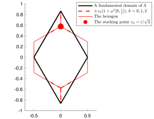
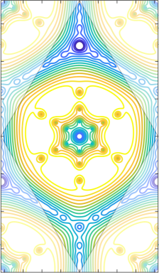
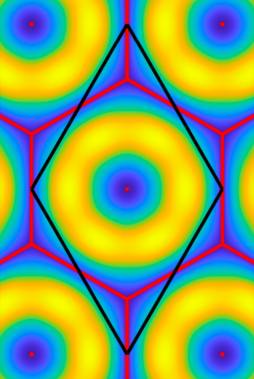
Figure 1. Left: the vertices of the hexagon in a fundamental domain of $\Lambda$ are given by the stacking points $\pm z_{S}$, $z_{S}=i/\sqrt{3}$. They are non-zero points of high symmetry in the sense that $\pm\omega z_{S}\equiv\pm z_{S}\!\!\mod\Lambda$. Center: plot of $\log|u_{K}(\alpha)|$ where $u_{K}$ is the protected state in the kernel of $D(\alpha)$ on $H^{1}(\mathbb{C}/\Gamma)$ and $\alpha=11.345$. Dark blue corresponds to $|u_{K}|\simeq 10^{-7}$ and yellow to $|u_{K}|\simeq 1$: we see exponential decay $e^{-c_{0}\alpha}$ near the hexagon and near its center. (This figure is borrowed from [Be*22].) Right: the contour plot of $|\{q,\bar{q}\}|_{q^{-1}(0)}|$ for $q$ given by the determinant of the semiclassical symbol of $D(\alpha)$ (see (1.1) and (1.2)), $\alpha=1/h$; the set where $\{q,\bar{q}\}|_{q^{-1}(0)}=0$ is in red. We should stress that the structure of that set becomes more complicated for other potentials $U$ satisfying the required symmetries - see §2.1 and [Be*22, Figure 6].

The natural asymptotic parameter is $\alpha\to\infty$, which corresponds to the small twisting angle limit (the angle is essentially given by $1/\alpha$). The operator $D(\alpha)$ is then a semiclassical operator with $h=1/\alpha\to 0$ playing the role of the semiclassical parameter.

A fascinating numerical observation about the asymptotic behaviour of real magic $\alpha$’s was made in [TKV19]: if $\alpha_{1}<\alpha_{2}<\cdots\alpha_{j}<\cdots$ is the sequence of all real $\alpha$’s for which (1.4) holds, then

$$\alpha_{j+1}-\alpha_{j}\simeq\tfrac{3}{2}.$$ (1.5)

This was based on a rough computation of $\alpha_{j}$ for $j\leq 8$. The spectral characterization of $\alpha$’s in [Be*22] allowed a finer computation, reliable for $j\leq 13$, and that suggested $\alpha_{j+1}-\alpha_{j}\simeq 1.515$ (this is so for the exact potential (1.2) with more complicated behaviour for potentials satisfying same symmetries but containing higher Fourier modes – see §2.1).

Although it is not clear if the model (1.1) is physically relevant for larger $\alpha$’s (or, for that matter, if more magic angles exist experimentally) establishing (1.5) remains a puzzling mathematical problem. It also remains of interest in physics [Re*21],[NaNa23] but the arguments and the proposed replacements to $\frac{3}{2}$ are not clear.

One of the difficulties in establishing (1.5) is the “exponential squeezing” of bands proved in [Be*22, Theorem 4]: for any $k\in\mathbb{C}$ and $\alpha\gg 1$, there exists $u\in C^{\infty}(\mathbb{C}/\Gamma)$ such that

$$\|(D(\alpha)+k)u\|_{L^{2}(\mathbb{C}/\Gamma)}\leq\mathcal{O}(e^{-c_{0}\alpha}),\ \ \|u\|_{L^{2}(\mathbb{C}/\Gamma)}=1,$$ (1.6)

that is, we have an almost eigenvalue at every $k$. This (and a much more precise statement) follows from the semiclassical version of Hörmander’s bracket condition - see Dencker–Sjöstrand–Zworski [DSZ04, Theorem 1.2^′] and references given there.

In view of (1.5) and (1.6) it is interesting to understand the precise behaviour of the exact solutions to the eigenvalue problem $(D(\alpha)+k)u=0$ as $\alpha$ gets large (within or without the magic set). As recalled in §2.1 that is equivalent to the study of the kernel of $D(\alpha)$ on $H^{1}(\mathbb{C}/\Gamma)$. Numerical simulations – see [Be*22, Figure 5] and the animation https://math.berkeley.edu/~zworski/magic.mp4 – suggest the presence of regions of exponential decay, $e^{-c_{0}\alpha}$, $c_{0}>0$, of the elements of that kernel. Although there is no classically forbidden region in the standard sense, some regions are forbidden in an infinitesimal way explained in Theorem 2 below. Our main result is

Theorem 1.

The hexagon spanned by the stacking points (see Figure 1) has an $\alpha$-independent neighbourhood $\Omega$ such that, for some constants $C_{0},c_{0}>0$ any solution of

$$(D(\alpha)+k)u=0,\ \ \ u\in H^{1}(\mathbb{C}/\Gamma;\mathbb{C}^{2}),\ \ \ \|u\|_{L^{2}(\mathbb{C}/\Gamma;\mathbb{C}^{2})}=1,$$ (1.7)

satisfies

$$|u(z)|\leq C_{0}e^{-c_{0}\alpha},\ \ \ z\in\Omega.$$ (1.8)

Remarks. 1. Near the interior of the edges of the hexagon, the theorem is based on a semiclassical Theorem 2 below and calculations involving the specific potential. At the corners a more direct argument is used in the Appendix, though the strategy and the method are the same. A much stronger estimate than (1.8), valid with all derivatives, holds – see (1.11). It should also be stressed that the result is local and we only need (1.7) to be valid in a neighbourhood of the hexagon.

2. An alternative approach to the analysis near the interior of the edges of the hexagon, or rather to the underlying microlocal result, Theorem 3 in §6 (see (1.12)), was recently developed by Sjöstrand [Sj23]. It provides an attractive alternative to the conjugation method (1.13) coming from [Sj82].

3. The situation is more complicated at the center, $z_{0}$, of the hexagon, where again we see exponential decay; there the operator is not even of principal type. In the notation of Theorem 2, $dq|_{q^{-1}(0)\cap\pi^{-1}(z_{0})}=0$. This suggests that lower order terms in (1.9) below are important. That is confirmed by the numerical study of a scalar model based on the leading term in (1.9): the principal terms agree but the absence of the lower order term produces no exponential decay at the center – see [GaZw23].

The crucial classical (or symplectic geometry) object in the formulation of Theorem 2 is the Poisson bracket: for $f,g\in C^{\infty}(\mathbb{R}^{2}_{x}\times\mathbb{R}^{2}_{\xi})$, where we think of $x$ as position and $\xi$ as momentum, the Poisson bracket is defined as

$$\{f,g\}=H_{f}\,g=\sum_{j=1}^{2}\partial_{\xi_{j}}f\,\partial_{x_{j}}g-\partial_{\xi_{j}}g\,\partial_{x_{j}}f.$$

Its significance comes from its appearance as the classical observable corresponding to the commutator of quantizations of $f$ and $g$ – see [Zw12, (4.3.11)].

The manifold $\mathbb{R}^{2}\times\mathbb{R}^{2}$ (or $U\times\mathbb{R}^{2}$ for $U\subset\mathbb{R}^{2}$ open) is identified with the (more invariant) cotangent bundle of $\mathbb{R}^{2}$, $T^{*}\mathbb{R}^{2}$ (or $T^{*}U$). We denote by $\pi:T^{*}U\rightarrow U$ the natural projection, $\pi(x,\xi)=x$.

Theorem 2.

Suppose that

$$P=Q\otimes I_{\mathbb{C}^{2}}+h\begin{pmatrix}R_{11}&R_{12}\\ R_{21}&R_{22}\end{pmatrix},\ \ \ x\in U\subset\mathbb{R}^{2},$$ (1.9)

is a principally scalar system of semiclassical differential operators with real analytic coefficients in $U$, $Q=q(x,hD_{x})$ is classically elliptic of order 2, and $R_{k\ell}=R_{k\ell}(x,hD_{x})$ are of order 1, for $1\leq k,\ell\leq 2$. Suppose that for $x_{0}\in U$, we have

$$\{q,\bar{q}\}|_{q^{-1}(0)\cap\pi^{-1}(x_{0})}=0,\ \ \ \{q,\{q,\bar{q}\}\}|_{q^{-1}(0)\cap\pi^{-1}(x_{0})}\neq 0,$$ (1.10)

and that $H_{\operatorname{Re}q}$ and $H_{\operatorname{Im}q}$ are linearly independent on $q^{-1}(0)\cap\pi^{-1}(x_{0})$. If $Pu=0$ in $U$ and $\|u\|_{L^{2}(U)}\leq\mathcal{O}(1)$, then there exists a neighbourhood $\Omega$ of $x_{0}$ and $C_{0},c_{0}>0$ such that for all $0<h\leq 1$ we have,

$$|\partial^{\beta}u(x)|\leq C_{0}(|\beta|C_{0})^{|\beta|}e^{-c_{0}/h},\ \ \ x\in\Omega,\ \ \beta\in\mathbb{N}^{2}.$$ (1.11)

Theorem 1 follows from Theorem 2 by considering the operator

$$P:=\alpha^{-2}(D(-\alpha)+k)(D(\alpha+k),\ \ \alpha=1/h.$$

The semiclassical principal symbol of $P$ is given by the determinant of the symbol of $\alpha^{-1}D(\alpha)$:

$$q(x,\xi)=(4\bar{\zeta})^{2}-U(z,\bar{z})U(-z,-\bar{z}),\ \ \ z=x_{1}+ix_{2},\ \ \bar{\zeta}=\tfrac{1}{2}(\xi_{1}+i\xi_{2}),$$

where we now stress the real analyticity of $U$ by writing it as the restriction to the totally real submanifold $\mathbb{C}\simeq\{(z,\bar{z}):z\in\mathbb{C}\}\subset\mathbb{C}^{2}$ of a function holomorphic in $\mathbb{C}^{2}$. For any fixed $z$, the range of $q(x,\xi)$ is $\mathbb{C}$ as $\xi$ varies, that is, there is no classically forbidden region in the standard sense. Similarly, if we consider Floquet theory (see §2.1) and look at the eigenfunctions of $H_{k}(\alpha):=e^{-i\langle k,z\rangle}H(\alpha)e^{i\langle k,z\rangle}$ in $H^{1}(\mathbb{C}/\Gamma;\mathbb{C}^{4})$, we see that the range of eigenvalues of the symbol on each fiber $T^{*}_{z}(\mathbb{C}/\Gamma)$ is $\mathbb{R}$.

The exponential decay near the hexagon is a consequence of the classical condition (1.10) which effectively determines a classically forbidden region for the eigenfunctions away from the vertices of the hexagon. The behaviour of $|\{q,\bar{q}\}|_{q^{-1}(0)}|$ is shown in Figure 1 – it can be considered as a function of $z$. As we already mentioned, [Be*22, Theorem 4] shows that near points where the bracket does not vanish we can construct localized pseudo-modes, $(D(\alpha)+k)u=\mathcal{O}(e^{-c_{0}\alpha})$, $\|u\|_{L^{2}}=1$, and this is indeed where the actual eigenfunctions concentrate (see the animation link above). For the animation showing $\log|u_{K}(\alpha)|$, where $u_{K}$ is the protected state satisfying $(D(\alpha)+K)u_{K}=0$, $\alpha=8e^{2\pi i\theta}$, $\|u_{K}\|_{L^{2}(\mathbb{C}/\Lambda)}=1$, and of the corresponding $|\{q,\bar{q}\}|_{q^{-1}(0)}|$, see https://math.berkeley.edu/~zworski/bracket_dynamics.mp4.

Recently, Sjöstrand and Vogel [SjVo23] have also investigated semiclassical properties of operators for which (1.10) holds and obtained delicate tunneling estimates in a model case in which separation of variables was possible. An extension of those results would likely have consequences for the operators we consider.

Theorem 2 is a consequence of the microlocal Theorem 3 in §6 and of the classical ellipticity of the operator $Q$ (see Proposition 6.4). Theorem 3 is in turn a semiclassical version of a theorem of Trépreau [Tr84] whose proof relied on ideas and methods introduced by Kashiwara and Kawai [KaKa79]. Himonas [Hi84] provided proofs of some of the results of Trépreau using Sjöstrand’s approach to analytic microlocal theory [Sj82], see also [HiSj15]. The results in [Tr84], [Hi84] were proved in the more complicated setting of analytic hypoellipticity but only for scalar operators. Here we are interested in a purely semiclassical statement which is valid for principally scalar systems. We specialize to dimension two but the statement and the methods of proof remain valid in all dimensions. We follow some aspects of [Hi84] but depart from that paper by using the full strength of [Sj82, Theorem 7.9] (see also Trépreau [Tr84]; the idea of using plurisubharmonic minorants is attributed to Kashiwara). We also avoid real analytic pseudodifferential operators and Egorov’s theorem for them, absorbing the real canonical transformation into an FBI transform.

We conclude this introduction by reviewing organization of the paper and outlining some aspects of the proof. In §2 we study the chiral model starting with a review of the flat band theory in §2.1 – this adds to the motivational discussion above. We then show how Theorem 1 follows from Theorem 2. In particular we find an explicit formula for $\{q,\{q,\bar{q}\}\}|_{q^{-1}(0)}$ on the open edges of the hexagon for the potential given by (1.2). At the corners of the hexagon, the bracket $\{q,\{q,\{q,\{q,\bar{q}\}\}\}\}|_{q^{-1}(0)}$ does not vanish but all shorter iterations of Poisson brackets are vanishing. The semiclassical analogue of [Tr84, Théorème 2] does not apply as the inequalities between “Egorov–Hörmander numbers” are not satisfied. By more ad hoc methods based on the specific structure of the symbol $q$ near the vertices, that case is covered in the Appendix.

§3 is devoted to microlocal preliminaries: definition of the semiclassical (analytic) wave front set of a distribution $u$, denoted $\operatorname{WF}_{h}(u)$ here, introduction of general FBI transforms, and a review of the invariance of the definition of the wave front set. The only slightly nonstandard fact is Proposition 3.3 which shows how to obtain FBI transform phase functions compatible with real analytic canonical transformations. In §4 we follow [Hi84] and obtain a real analytic symplectic reduction of the symbol to an approximation of a model case $\xi_{1}+i(x_{1}^{2}+\xi_{2})$. This follows a long tradition in the subject – see [Hö3, §21.3]. §5 provides a solution of the complex eikonal equation associated to the approximate model symbol. That involves a rescaling similar to that in [Hi84]. It also provides the analysis of the associated weights – see (1.14) below.

The proof of a microlocal version of Theorem 2 is given in §6 and relies on the analysis in §5. The goal is to show that

$$\begin{gathered}q(\rho)=0,\ \ dq\!\not\,\parallel\!d\bar{q},\ \ \{q,\bar{q}\}(\rho)=0,\\ \{q,\{q,\bar{q}\}\}(\rho)\neq 0,\ \ \rho\notin{\rm{WF}}_{h}(Pu)\end{gathered}\ \Bigg{\}}\ \Longrightarrow\ \rho\notin{\rm{WF}}_{h}(u).$$ (1.12)

For that we use the phase function from §5 to construct an FBI transform $T_{h}$ (incorporating the canonical transformation from §4 using Proposition 3.3) such that, for our system $P$,

$$T_{h}P\equiv hD_{x_{1}}T_{h}.$$ (1.13)

(The equivalence here is formulated using exponentially weighted spaces of holomorphic functions, see (3.3).) This is done for systems such as (1.9).

The phase of this new FBI transform satisfies the (holomorphic) eikonal equation

$$\partial_{x_{1}}\varphi(x,y)=q(y,-\partial_{y}\varphi(x,y)),\ \ \ \Phi(x):=\sup_{y\in\operatorname{neigh}_{\mathbb{R}^{2}}(y_{0})}-\operatorname{Im}\varphi(x,y),$$ (1.14)

where $q$ is the principal symbol of $Q$ in (1.9) and $\rho=(y_{0},\eta_{0})\in T^{*}\mathbb{R}^{2}$ satisfies the condition in (1.12). We have for all $\varepsilon>0$,

$$|T_{h}u(x)|\leq C_{\varepsilon}\exp((\Phi(x)+\varepsilon)/h),\ \ x\in\operatorname{neigh}_{\mathbb{C}^{2}}(x_{0}),\ \ x_{0}=\pi(\kappa_{\varphi}(\rho)),$$ (1.15)

where $\kappa_{\varphi}$ is the complex symplectomorphism associated to $\varphi$ – see (3.10). The key fact is that the wave front set is independent of the choice of $\varphi$ – see [HiSj15, Proposition 2.6.4] and Proposition 3.2 below. Hence to obtain (1.12), we need to show that we have an exponential improvement over (1.15), that is, that for some $\delta>0$,

$$|T_{h}u(x)|\leq C\exp((\Phi(x)-\delta)/h),\ \ x\in\operatorname{neigh}_{\mathbb{C}^{2}}(x_{0}),\ \ x_{0}=\pi(\kappa_{\varphi}(\rho)).$$ (1.16)

Assuming for simplicity that $Pu=0$ and that $x_{0}=0$, (1.13) shows that $T_{h}u(x)$ is essentially independent of $x_{1}$. This means that the weight $\Phi(x)$ in (1.15) can be replaced by its minimum over $x_{1}\in\operatorname{neigh}_{\mathbb{C}}(0)$, The key idea, attributed to Kashiwara in [Tr84] (though implemented there using different technology), is to prove that for some fixed $\delta>0$ we have,

$$\text{ $\Psi(x_{2})\leq\min_{|x_{1}|\leq\varepsilon}\Phi(x)$ and $\Psi(x_{2})$ is subharmonic}\ \Longrightarrow\ \Psi(0)\leq\Phi(0)-\delta.$$ (1.17)

That is done in Lemma 5.2. Applying (1.17) to $\Psi(x_{2}):=h\log|T_{h}u(0,x_{2})|$ gives (1.16).

Finally, we pass from the microlocal statement (1.12) (Theorem 3) to an exponential decay statement (1.11). That relies on the classical ellipticity of the operator $P$ and is given in Proposition 6.4. Although seemingly standard we could not find a reference for the semiclassical case and relied on recent work by Galkowski–Zworski [GaZw21],[GaZw22] (based on [HeSj86], [Sj96]) to give a short proof.

The appendix, which is the joint work of Zhongkai Tao and the second-named author, treats the case of the corners of the hexagon, that is, in physical nomenclature, neighbourhoods of stacking points – see Figure 1. We follow the same procedure but use the special structure of $q=(2\bar{\zeta})^{2}-U(z)U(-z)$ near $z=z_{S}$. That allows an explicit analysis of a solution to (1.14) without taking a preparatory canonical transformation. We obtain (1.17) for the corresponding weight and the same method applies.

Acknowledgements. We would like to thank Johannes Sjöstrand for helpful conversations and in particular for directing us to the work of Trépreau [Tr84] and to [Sj82, Theorem 7.9]. We are also grateful to Mark Embree for help with Figure 1 and to Simon Becker for the linked movies. This work has been partially supported by the Simons Targeted Grant Award No. 896630, “Moiré Materials Magic” .

2. Reduction to Theorem 2

We first review some basic facts about symmetries of $D(\alpha)$ and flat bands for the model (1.1). We then discuss the reduction to an operator of the type appearing in Theorem 2. Finally, we show that bracket conditions (1.10) hold at the interior points of the edges of the hexagon spanned by the stacking points (see Figure 1) and discuss properties of the Poisson brackets at the corners.

2.1. Flat bands and protected states

The potential $U$ in (1.2) enjoys the following symmetries with respect to the lattice in (1.3), the rotation by $2\pi/3$, and complex conjugation:

$$U(z+\gamma)=e^{i\langle\gamma,K\rangle}U(z),\ \gamma\in\Lambda,\quad U(\omega z)=\omega U(z),\ \ \overline{U(\bar{z})}=-U(-z).$$ (2.1)

The operator $D(\alpha)$ (and the self-adjoint Hamiltonian $H(\alpha)$) are periodic with respect to $\Gamma=3\Lambda$ and assumptions (2.1) are enough to guarantee that there exists a discrete set $\mathcal{A}\subset\mathbb{C}$ such that for $D(\alpha)$ with the domain given by $H^{1}(\mathbb{C}/\Gamma)$,

$$\operatorname{Spec}_{L^{2}(\mathbb{C}/\Gamma)}D(\alpha)=\left\{\begin{array}[]{ll}\Gamma^{*},&\alpha\notin\mathcal{A},\\ \mathbb{C},&\alpha\in\mathcal{A},\end{array}\right.$$

see [Be*22, Theorem 2] and for a finer version using the lattice $\Lambda$, [BHZ22b, Proposition 2.2]. For $\alpha\notin\mathcal{A}$,

$$\dim\ker_{H^{1}(\mathbb{C}/\Gamma)}D(\alpha)=2,$$

and the spectrum of $D(\alpha)$ is periodic with respect to $\Gamma^{*}$ – see [Be*22, Theorem 1] or [BHZ22b, Proposition 2.1].

The bands of the Hamiltonian $H(\alpha)$ are defined as the eigenvalues of $H_{k}(\alpha):=e^{-i\langle z,k\rangle}H(\alpha)e^{i\langle z,k\rangle}$, $\langle z,k\rangle:=\operatorname{Re}(\bar{z}k)$, with the domain $H^{1}(\mathbb{C}/\Gamma)$ (for a finer description see [BHZ22b]). Since these eigenvalues are symmetric with respect to $0$ and at $k=0$, the protected states give a multiplicity four eigenvalue at $0$, we can write the spectrum as

$$\operatorname{Spec}_{L^{2}(\mathbb{C}/\Gamma;\mathbb{C}^{4})}H_{k}(\alpha)=\{E_{j}(\alpha,k)\}_{j\in\mathbb{Z}\setminus\{0\}},\ \ \ E_{\pm j}(\alpha,0)=0,\ \ j=1,2.$$

Bloch–Floquet theory shows that if we consider $H(\alpha)$ with domain given by $H^{1}(\mathbb{C};\mathbb{C}^{4})$, then

$$\operatorname{Spec}_{L^{2}(\mathbb{C})}H(\alpha)=\bigcup_{k\in\mathbb{C}/\Gamma^{*}}\{E_{j}(\alpha,k)\}_{j\in\mathbb{Z}\setminus\{0\}}.$$

A flat band at $0$ corresponds to

$$E_{\pm j}(\alpha,k)=0\ \text{ for all $k\in\mathbb{C}$, $j=1,2$. }$$ (2.2)

The definition of $H_{k}(\alpha)$ above shows that this is equivalent to $\operatorname{Spec}_{L^{2}(\mathbb{C}/\Gamma)}D(\alpha)=\mathbb{C}$ and the eigenfunctions are given by

$$\begin{gathered}\begin{pmatrix}u(k)\\ u^{*}(k)\end{pmatrix}\in C^{\infty}(\mathbb{C}/\Gamma;\mathbb{C}^{4}),\\ (D(\alpha)+k)u(k)=0,\ \ \ (D(\alpha)^{*}+\bar{k})u^{*}(k)=0,\ \ u(k),u^{*}(k)\in C^{\infty}(\mathbb{C}/\Gamma;\mathbb{C}^{2}).\end{gathered}$$

The functions $u(k)$ and $u^{*}(k)$ are easily related to each other (see for instance [BHZ22b, (2.10)]) and in addition the functions $z\mapsto|u(k,z)|$ are periodic with respect to the the small lattice $\Lambda$ (see (1.3)). Hence when looking for “classically forbidden” regions for $u(k)$ (as $\alpha\to\infty$) we can consider the fundamental domain of $\Lambda$ shown in Figure 1. Using the “theta function argument” (see [BHZ22b, §3]) $u(k)$ can be obtained from the $u(0)$. Hence, we are effectively looking for classically forbidden regions of the protected elements of the kernel of $D(\alpha)$ – see https://math.berkeley.edu/~zworski/magic.mp4.

2.2. Reduction to the principally scalar case

We start by noting that $D(-\alpha)$ is the (formal) adjugate matrix of $D(\alpha)$ and

$$\begin{gathered}(D(-\alpha)+k)(D(\alpha)+k)=Q_{k}(\alpha)\otimes I_{\mathbb{C}^{2}}+\alpha R_{k}(\alpha)=:P_{k}(\alpha),\\ Q_{k}(\alpha)=(2D_{\bar{z}})^{2}-\alpha^{2}U(z)U(-z),\\ R_{k}(\alpha)=\begin{pmatrix}k\alpha^{-1}4D_{\bar{z}}+k^{2}\alpha^{-1}&2D_{\bar{z}}U(z)\\ -(2D_{\bar{z}}U)(-z)&k\alpha^{-1}4D_{\bar{z}}+k^{2}\alpha^{-1}\end{pmatrix}.\end{gathered}$$ (2.3)

In particular if $u\in\ker_{L^{2}(\mathbb{C}/\Gamma)}(D(\alpha)+k)$ then $(Q_{k}(\alpha)\otimes I_{\mathbb{C}^{2}}+\alpha R_{k}(\alpha))u=0$.

Remark. We recall from [Be*22] that $\alpha$ is magical if and only if $\ker_{L^{2}(\mathbb{C}/\Gamma)}(D(\alpha)+k)\neq\{0\}$ for some $k\notin\Gamma^{*}=\frac{1}{3}\Lambda^{*}$. That is equivalent to $\ker_{L^{2}(\mathbb{C}/\Gamma)}P_{k}(\alpha)\neq\{0\}$, for some $k\notin\frac{1}{3}\Lambda^{*}$. In fact, if $u\in\ker_{L^{2}(\mathbb{C}/\Gamma)}(D(\alpha)+k)$ then obviously $P_{k}(\alpha)u=0$. On the other hand if $P_{k}(\alpha)u=0$ and $v:=(D(\alpha)+k))u\neq 0$ then $(D(-\alpha)+k))v=0$. Since

$$D(-\alpha)=-\mathscr{R}D(\alpha)\mathscr{R},\ \ \ \mathscr{R}\begin{pmatrix}u_{1}\\ u_{2}\end{pmatrix}(z)=\begin{pmatrix}u_{2}(-z)\\ u_{1}(-z)\end{pmatrix},$$

we have $\mathscr{R}v\in\ker_{L^{2}(\mathbb{C}/\Gamma)}(D(\alpha)-k)$, $-k\notin\frac{1}{3}\Lambda^{*}$, that is, $\alpha$ is magical. ∎

We now take a semiclassical point of view [Zw12], put $h:=1/\alpha$, and define

$$\begin{gathered}P=h^{2}P_{k}(\alpha)=Q\otimes I_{\mathbb{C}^{2}}+hR,\\ Q:=(2hD_{\bar{z}})^{2}-U(-z)U(z)=q(x,hD_{x}),\\ q(x,\xi)=(\xi_{1}+i\xi_{2})^{2}-V(x),\ \ \ V(x)=U(z)U(-z),\ \ \ z=x_{1}+ix_{2},\\ R=\begin{pmatrix}\ \ \ k4hD_{\bar{z}}+hk^{2}&2D_{\bar{z}}U(z)\\ -(2D_{\bar{z}}U)(-z)&\ \ k4hD_{\bar{z}}+hk^{2}\end{pmatrix},\end{gathered}$$ (2.4)

which is the form of the operator in Theorem 2, provided that $k\in\mathbb{C}$ is confined to a fixed bounded set. We now verify that assumption (1.10) is satisfied for $x_{0}$ on the open edges of the hexagon in Figure 1.

2.3. Bracket computations

It is convenient to use the complex notation $\zeta=\frac{1}{2}(\xi_{1}-i\xi_{2})$, $\partial_{\zeta}=\partial_{\xi_{1}}+i\partial_{\xi_{2}}$, $z=x_{1}+ix_{2}$, so the real symplectic form on $T^{*}\mathbb{R}^{2}$ is given by

$$2\operatorname{Re}d\zeta\wedge dz=d\zeta\wedge dz+d\bar{\zeta}\wedge d\bar{z}.$$ (2.5)

Consequently, the Poisson bracket is given by

$$\{a,b\}=\sum_{j=1}^{2}\partial_{\xi_{j}}a\,\partial_{x_{j}}b-\partial_{\xi_{j}}b\,\partial_{x_{j}}a=\partial_{\zeta}a\,\partial_{z}b-\partial_{\zeta}b\,\partial_{z}a+\partial_{\bar{\zeta}}a\,\partial_{\bar{z}}b-\partial_{\bar{\zeta}}b\,\partial_{\bar{z}}a.$$ (2.6)

We then have (strictly speaking we should write $V=V(z,\bar{z})$),

$$q=4\bar{\zeta}^{2}-V(z),\ \ \ V(z)=U(z)U(-z),\ \ \ U(z)=\lambda i\sum_{\ell=0}^{2}\omega^{\ell}e^{i\langle z,\omega^{\ell}K\rangle},$$ (2.7)

where $K=\tfrac{4}{3}\pi$, and we introduced a general coupling constant $\lambda$. If $\lambda\in\mathbb{R}$ (which is the case for (1.2)) then,

$$\overline{U(\bar{z})}=-U(-z),\ \ \ \overline{V(\bar{z})}=V(z)=V(-z).$$ (2.8)

In particular, when $t\in\mathbb{R}$, then $\operatorname{Im}V(it)=0$, $\operatorname{Re}U(it)=0$. Also, $\partial_{z}U(z)=-\frac{1}{2}K\lambda\sum_{\ell=0}^{2}e^{i\langle z,\omega^{\ell}K\rangle}$, so

$$\begin{gathered}\overline{(\partial_{z}U)(\bar{z})}=(\partial_{z}U)(-z),\ \ \ \overline{\partial_{z}V(\bar{z})}=-(\partial_{z}V)(-z),\end{gathered}$$ (2.9)

and in particular, $\operatorname{Re}\partial_{z}V(it)=0$ for $t\in\mathbb{R}$.

The next two lemmas show that the conditions in Theorem 2 are satisfied for the principal symbol of the operator $P$ in (2.4). They are illustrated numerically in Figure 2.

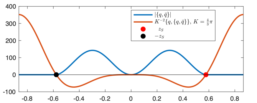
Figure 2. Plots of $|\{q,\bar{q}\}|$ and of (rescaled) $\{q,\{q,\bar{q}\}\}$ above the intersection of the imaginary axis and the fundamental domain in Figure 1. The edges of the hexagon emanate right of $z_{S}$ and left of $-z_{S}$.

Lemma 2.1.

Let

$$H:=\cup_{\pm}\cup_{k=0}^{2}\pm(1+\omega^{k}[0,\tfrac{1}{2}])i/\sqrt{3}+\Lambda,$$

be the hexagon spanned by the stacking points $\pm z_{S}+\Lambda$, $z_{S}=i/\sqrt{3}$ (see Figure 1). Then $q$ given in (2.7) with $\lambda\in\mathbb{R}$ satisfies

$$\{q,\bar{q}\}(\rho)=0\ \text{ if }\ z\in H,\ \rho\in\pi^{-1}(z)\cap q^{-1}(0),$$ (2.10)

where $\pi:T^{*}(\mathbb{C}/\Lambda)\rightarrow\mathbb{C}/\Lambda$ is the natural projection, $\pi(z,\zeta)=z$.

Proof.

We note some basic symmetries relevant to the hexagon. We define the following symplectomorphism (for the standard real symplectic form (2.5); it also preserves the complex one $d\zeta\wedge dz$):

$$R:(z_{S}+z,\bar{z}_{S}+\bar{z},\zeta,\bar{\zeta})\longmapsto(z_{S}+\omega z,\bar{z}_{S}+\bar{\omega}\bar{z},\bar{\omega}\zeta,\omega\bar{\zeta}).$$ (2.11)

Then,

$$R^{*}q=\omega^{2}q,\ \ \ R^{*}\{q,\bar{q}\}=\{q,\bar{q}\},\ \ \ R^{*}\{q,\{q,\bar{q}\}\}=\omega^{2}\{q,\{q,\bar{q}\}\}.$$ (2.12)

Hence it is enough to check (2.10) for $z\in z_{S}[1,\frac{3}{2}]$. Since

$$H_{q}=8\bar{\zeta}\partial_{\bar{z}}+\partial_{z}V\partial_{\zeta}+\partial_{\bar{z}}V\partial_{\bar{\zeta}},$$ (2.13)

we have, when $q=0$,

$$\{q,\bar{q}\}=8\zeta\partial_{z}V-8\bar{\zeta}\overline{\partial_{z}V}=16i\operatorname{Im}(\zeta\partial_{z}V)=\pm 8i\operatorname{Im}\left((\overline{V(z)})^{\frac{1}{2}}\partial_{z}V(z)\right),$$ (2.14)

where $\pm$ depends on $2\bar{\zeta}=\mp(V(z))^{\frac{1}{2}}$ (so that $q=0$). From (2.8) and (2.9) we see that $V$ is real and $\partial_{z}V$ is purely imaginary on $i\mathbb{R}$, and it remains to show that $V(it)<0$ for $1/\sqrt{3}<\pm t\leq\sqrt{3}/2$. For that we calculate

$$U(it)=i\lambda\sum_{\ell=0}^{2}\omega^{\ell}e^{\frac{i}{2}K(it\bar{\omega}^{\ell}-it\omega^{\ell})}=\lambda i(1+2\cos(2\pi(t\sqrt{3}+1)/3)).$$

This means that we need

$$\left(1+2\cos\left({2\pi}(1+t\sqrt{3})/3\right)\right)\left(1+2\cos\left(2\pi(1-t\sqrt{3})/3\right)\right)>0,$$ (2.15)

for $1/\sqrt{3}<t\leq\sqrt{3}/2$. Writing $2\pi(1+t\sqrt{3})/3=\pi+\theta$, ${\pi}/{3}<\theta\leq 2\pi/{3}$, it follows that

$$1+2\cos\left({2\pi}(1+t\sqrt{3})/3\right)=1-2\cos\theta>0.$$

Similarly, with ${2\pi}(1-t\sqrt{3})/3=\theta$ , $-{\pi}/{3}\leq\theta<0,$ we obtain

$$1+2\cos\left({2\pi}(1-t\sqrt{3})/3\right)=1+2\cos\theta>0,$$

and (2.15) follows. ∎

Lemma 2.2.

For the potential given in (1.2) and for $z\in\pm(z_{S}+\omega^{k}(0,\frac{1}{2}z_{S}])$, $z_{S}=i/\sqrt{3}$, $0\leq k\leq 2$ (open edges of the hexagon), $H_{{\rm Re}\,q}(\rho)$, $H_{{\rm Im}\,q}(\rho)$ are linearly independent for $\rho\in\pi^{-1}(z)\cap q^{-1}(0)$. Furthermore,

$$\omega^{2k}\{q,\{q,\bar{q}\}\}(\rho)>0,\ \ \ \rho\in\pi^{-1}(z)\cap q^{-1}(0).$$ (2.16)

Proof.

As in the proof of Lemma 2.1, we use (2.12) so that it is enough to consider $z=it$, $1/\sqrt{3}<\pm t\leq\sqrt{3}/2$. First, the linear independence of the Hamilton vector fields $H_{{\rm Re}\,q}(\rho)$, $H_{{\rm Im}\,q}(\rho)$ follows from (2.13), combined with the fact that $V(it)<0$ for $1/\sqrt{3}<\pm t\leq\sqrt{3}/2$, established in the proof of Lemma 2.1. Next, from (2.13) we see that, at points $\in q^{-1}(0)\cap\pi^{-1}(it)$,

$$\begin{split}\{q,\{q,\bar{q}\}\}&=(8\bar{\zeta}\partial_{\bar{z}}+\partial_{z}V\partial_{\zeta}+\partial_{\bar{z}}V\partial_{\bar{\zeta}})(8\zeta\partial_{z}V-8\bar{\zeta}\overline{\partial_{z}V})\\ &=64(|\zeta|^{2}\partial_{z}\partial_{\bar{z}}V-\bar{\zeta}^{2}\overline{\partial_{z}^{2}V})+8((\partial_{z}V)^{2}-\partial_{\bar{z}}V\overline{\partial_{z}V}).\\ &=16(|V|\partial_{z}\partial_{\bar{z}}V-V\overline{\partial_{z}^{2}V})+8((\partial_{z}V)^{2}-\partial_{\bar{z}}V\overline{\partial_{z}V})\\ &=-16V(\partial_{z}\partial_{\bar{z}}V+\overline{\partial_{z}^{2}V})+8((\partial_{z}V)^{2}-\partial_{\bar{z}}V\overline{\partial_{z}V}).\end{split}$$ (2.17)

where we again used that $V(it)<0$ for $1/\sqrt{3}<\pm t\leq\sqrt{3}/2$. A computation based on (2.7) shows that

$$\begin{gathered}\partial_{\bar{z}}U(z)=\tfrac{1}{2}iKU(\bar{z}),\ \ \ \partial_{z}^{2}U(z)=-\tfrac{1}{4}K^{2}U(\bar{z}).\end{gathered}$$ (2.18)

Hence, using also $\partial_{z}\left(U(\bar{z})\right)=(\partial_{\bar{z}}U)(\bar{z})$ and $\partial_{z}\left(U(-\bar{z})\right)=-(\partial_{\bar{z}}U)(-\bar{z})$, we obtain

$$\begin{split}\partial_{z}V(z)&=\partial_{z}U(z)U(-z)-(\partial_{z}U)(-z)U(z),\\ \partial_{\bar{z}}V(z)&=\partial_{\bar{z}}U(z)U(-z)-(\partial_{\bar{z}}U)(-z)U(z)=\tfrac{1}{2}iK\left(U(\bar{z})U(-z)-U(-\bar{z})U(z)\right),\\ \partial_{z\bar{z}}^{2}V(z)&=\tfrac{1}{2}iK\left((\partial_{\bar{z}}U)(\bar{z})U(-z)-U(\bar{z})(\partial_{z}U)(-z)+(\partial_{\bar{z}}U)(-\bar{z})U(z)-U(-\bar{z})\partial_{z}U(z)\right)\\ &=-\tfrac{1}{2}K^{2}U(z)U(-z)-\tfrac{1}{2}iK\left((\partial_{z}U)(-z)U(\bar{z})+\partial_{z}U(z)U(-\bar{z})\right),\\ \partial_{z}^{2}V(z)&=\partial_{z}^{2}U(z)U(-z)+(\partial_{z}^{2}U)(-z)U(z)-2\partial_{z}U(z)(\partial_{z}U)(-z)\\ &=-\tfrac{1}{4}K^{2}\left(U(\bar{z})U(-z)+U(-\bar{z})U(z)\right)-2\partial_{z}U(z)(\partial_{z}U)(-z).\end{split}$$

We now put

$$\begin{gathered}f(t):=U(it),\ \ g(t):=\partial_{z}U(it),\ \ \ \ \bar{f}(t)=-f(t),\ \ \bar{g}(t)=g(t),\ \ g(t)=g(-t)\\ f(t)=i\lambda(1+2\cos(2\pi(t\sqrt{3}+1)/3)),\ \ \ g(t)=-\tfrac{1}{2}K\lambda(1+2\cos(2\pi t\sqrt{3}/3)).\end{gathered}$$ (2.19)

To simplify notation further we take (as we may) $\lambda=1$ and denote $c:=\cos(2\pi t\sqrt{3}/3)$ and $s:=\sqrt{3}\sin(2\pi t\sqrt{3}/3)$, so that

$$g(t)=-\tfrac{1}{2}K(1+2c),\ \ f(t)=i(1-c-s),\ \ f(-t)=i(1-c+s).$$

Then, using the fact that $s^{2}=3(1-c^{2})$, a lengthy computation gives

$$\begin{split}\tfrac{1}{8}K^{-2}\{q,\{q,\bar{q}\}\}&=(c-1)^{2}(2c+1)(2c-9).\end{split}$$

For $1/\sqrt{3}<t\leq\sqrt{3}/2$, $-1\leq c=\cos(2\pi\sqrt{3}t/3)<-\frac{1}{2}$. Hence $c-1,2c+1,2c-9<0,$ and $\{q,\{q,\bar{q}\}\}>0$, as claimed. ∎

We conclude this section by recording the behaviour of the Poisson brackets at the vertices of the hexagon, where Theorem 2 does not apply. We note first that

$$\begin{gathered}U(z_{S})=0,\ \ \partial_{z}U(z_{S})=0,\ \ \partial_{\bar{z}}U(z_{S})=\tfrac{8}{3}\pi^{2},\\ U(-z_{S})=-4\pi i,\ \ \partial_{z}U(-z_{S})=0,\ \ \partial_{\bar{z}}U(-z_{S})=0.\end{gathered}$$ (2.20)

Hence,

$$\pi^{-1}(\pm z_{S})\cap q^{-1}(0)=\{(\pm z_{S},0)\},\ \ \ dq(\pm z_{S},0)=\pm\tfrac{32}{3}\pi^{3}i\,d\bar{z}\neq 0.$$

Lemma 2.3.

We have

$$H_{q_{j_{1}}}\cdots H_{q_{j_{p}}}\bar{q}\,(\pm z_{S},0)=0,\ p<4,\ \ \forall\,j_{\ell}\in\{1,2\},\ \ q_{1}=q,\ q_{2}=\bar{q},$$ (2.21)

and

$$H_{q}^{4}\bar{q}\,(\pm z_{S},0)=\{q,\{q,\{q,\{q,\bar{q}\}\}\}\}(\pm z_{S},0)\neq 0.$$ (2.22)

Proof.

Since $q$ is even in $z$ it is enough to consider $z_{S}$. Using (2.18) and (2.20) we see that that $V(z+z_{S})=U(-z_{S})\partial_{\bar{z}}U(z_{S})\bar{z}+\frac{1}{2}U(-z_{S})\partial_{z}^{2}U(z_{S})z^{2}+\mathcal{O}(|z|^{3})$, so that

$$p(z,\zeta):=\tfrac{1}{8}q(z_{S}+z,\zeta)=\tfrac{1}{2}\bar{\zeta}^{2}-a\bar{z}-\tfrac{1}{2}bz^{2}+\mathcal{O}(|z|^{3}),\ \ \ a=-\tfrac{4}{3}\pi^{3}i,\ \ b=\tfrac{8}{9}\pi^{4}.$$ (2.23)

Consequently,

$$H_{p}=\bar{\zeta}\partial_{\bar{z}}+a\partial_{\bar{\zeta}}+bz\partial_{\zeta}+\mathcal{O}(|z|^{2})\partial_{\zeta}+\mathcal{O}(|z|^{2})\partial_{\bar{\zeta}}.$$

Then $H_{p}\bar{p}=-b\bar{z}\bar{\zeta}+bz\zeta+\mathcal{O}(|z|^{2}|\zeta|)$, and

$$\begin{split}H_{p}^{2}\bar{p}&=-b\bar{\zeta}^{2}-ab\bar{z}+\mathcal{O}(|z||\zeta|^{2}+|z|^{2}),\\ H_{p}^{3}\bar{p}&=-3ab\bar{\zeta}+\mathcal{O}(|z||\zeta|+|\zeta|^{3}+|z|^{2}),\\ H_{p}^{4}\bar{p}&=-3a^{2}b+\mathcal{O}(|\zeta|+|z|)\neq 0,\ \ 0\leq|z|,|\zeta|\ll 1.\end{split}$$

This proves (2.22) and part of (2.21). Since $H_{p}\bar{p}$ is purely imaginary, we have,

$$H_{\bar{p}}H_{p}\bar{p}=-\overline{H_{p}^{2}\bar{p}},\ \ \ H_{\bar{p}}^{2}H_{p}\bar{p}=-\overline{H_{p}^{3}\bar{p}},\ \ \ H_{p}H_{\bar{p}}H_{p}\bar{p}=-\overline{H_{\bar{p}}H_{p}^{2}\bar{p}}$$

so the only remaining case to check is $H_{\bar{p}}H_{p}^{2}\bar{p}$, and that is again straightforward. ∎

3. Microlocal preliminaries

We review aspects of microlocal analysis needed in the proof of Theorem 2.

3.1. Analytic symbols

In the semiclassical setting we work locally and consider functions defined in open sets (typically neighbourhoods of fixed points) $\Omega\subset\mathbb{C}^{N}$. For a continuous function $\Phi:\Omega\to\mathbb{R}$ (typically plurisubharmonic), Sjöstrand spaces (following terminology of Lebeau [Leb85]), $H_{\Phi}(\Omega)$, are defined as spaces of functions $u:\Omega\times(0,1]\to\mathbb{C}$, satisfying

$$u(\bullet,h)\in\mathscr{O}(\Omega),\ \ \forall\,K\Subset\Omega,\ \varepsilon>0\ \exists\,C\ \forall\,h\in(0,1]\ \forall\,z\in K\ \ |u(z,h)|\leq Ce^{(\Phi(z)+\varepsilon)/h}.$$ (3.1)

For $z_{0}\in\Omega$ and $\Phi\in C(\Omega)$ we also define the space of germs at $z_{0}$:

$$H_{\Phi,z_{0}}:=\bigcup_{\Omega^{\prime}=\operatorname{neigh}_{\mathbb{C}^{N}}(z_{0})\subset\Omega}H_{\Phi}(\Omega^{\prime}).$$ (3.2)

The equivalence relations on these spaces are given as follows:

$$\begin{gathered}u\equiv_{H_{\Phi}(\Omega)}v\ \Longleftrightarrow\ \exists\,\Phi_{0}\in C(\Omega),\ \Phi_{0}<\Phi\ \ u-v\in H_{\Phi_{0}}(\Omega),\\ u\equiv_{H_{\Phi,z_{0}}}v\ \Longleftrightarrow\ \exists\,\Omega^{\prime}=\operatorname{neigh}_{\mathbb{C}^{N}}(z_{0})\subset\Omega,\ u,v\in H_{\Phi}(\Omega^{\prime})\ \text{and}\ \ u\equiv_{H_{\Phi}(\Omega^{\prime})}v.\end{gathered}$$ (3.3)

When the context is clear we may drop $\bullet$ in $\equiv_{\bullet}$ or write $\equiv$ in $\bullet$.

Analytic symbols in $\Omega$ are defined using $\Phi=0$: they are given by the space $H_{0}(\Omega)$. A (formal) classical analytic symbol in $\Omega$ is a (formal) expression

$$\begin{gathered}a(z;h):=\sum_{k=0}^{\infty}h^{k}a_{k}(z),\ \ a_{k}\in\mathscr{O}(\Omega),\\ \forall\,K\Subset\Omega\,\,\exists\,C=C(K)\ \ |a_{k}(z)|\leq C^{k+1}k^{k},\ z\in K,\,\,k=0,1,2,\ldots.\end{gathered}$$ (3.4)

For open $\Omega_{1}\Subset\Omega$ we have a realization of $a(z;h)$ given by the following holomorphic function:

$$a_{\Omega_{1}}(z;h):=\sum_{k=0}^{[(eC(\Omega_{1})h)^{-1}]}a_{k}(z)h^{k},\ \ \Omega_{1}\subset\Omega_{2}\Subset\Omega\ \Rightarrow\ a_{\Omega_{1}}\equiv a_{\Omega_{2}}\text{ in }H_{0}(\Omega_{1}).$$ (3.5)

We refer to [Sj82, §1] or [HiSj15, §2.2] for a detailed account. We recall however the following fundamental result of Boutet de Monvel–Krée. The composition of symbols defined there is motivated by the composition formula for pseudodifferential operators.

Proposition 3.1.

For $a=a(x,\xi;h)$ and $b=b(x,\xi;h)$, formal classical analytic symbols in $\Omega\subset\mathbb{C}_{x}^{n}\times\mathbb{C}_{\xi}^{n}$ we define

$$a\#b(x,\xi;h):=\sum_{\alpha\in\mathbb{N}^{n}}\frac{1}{\alpha!}\partial_{\xi}^{\alpha}a(x,\xi;h)(hD_{x})^{\alpha}b(x,\xi;h).$$ (3.6)

Then $a\#b$ is a classical analytic symbol in $\Omega$. If $a\neq 0$ on $\Omega$ and $\Omega_{0}\Subset\Omega$ is an open set, then the formal classical symbol $b$ defined by

$$a\#b=1$$ (3.7)

is a formal classical analytic symbol in $\Omega_{0}$.

The condition that $a\neq 0$ in $\Omega$ is referred to as the ellipticity of $a$ in $\Omega$.

3.2. Analytic semiclassical wave front sets

Let $U$ be an open set in $\mathbb{R}^{n}$, and suppose that ${(0,h_{0}]\ni}h\mapsto u(h)\in\mathscr{D}^{\prime}(U;\mathbb{C}^{p})$ is a family of vector-valued $h$-tempered distributions in the sense that for every $\omega\Subset U$ there exists $N$ such that $\|u(h)\|_{H^{-N}(\omega)}=\mathcal{O}(h^{-N})$. We follow [Ma02, Definition 3.2.1] and define the semiclassical analytic wave front set, $\operatorname{WF}_{h}(u)\subset T^{*}U$, as follows:

$$\begin{gathered}(y_{0},\eta_{0})\notin\operatorname{WF}_{h}(u)\ \Longleftrightarrow\ \left\{\begin{array}[]{l}\exists\,\delta>0,C>0,\ \Omega=\operatorname{neigh}_{\mathbb{C}^{n}}(y_{0}-i\eta_{0})\\ |T_{h}u(x)|\leq Ce^{(\Phi_{0}(x)-\delta)/h},\ x\in\Omega,\,\,0<h\leq h_{0},\end{array}\right.\\ T_{h}w(x):=\int_{\mathbb{R}^{n}}w(y)\chi(y)e^{i\varphi_{0}(x,y)/h}dy,\ \ \varphi_{0}(x,y):=i(x-y)^{2}/2,\ \ \Phi_{0}(x):=\tfrac{1}{2}|\operatorname{Im}x|^{2},\end{gathered}$$ (3.8)

where $\chi\in C^{\infty}_{\rm{c}}(U)$, $\chi({y})\equiv 1$ in a neighbourhood of $y_{0}$. (We should note that for $h$-independent distributions $u$ this gives the analytic wave front set $\operatorname{WF}_{\rm{a}}(u)$, [HöI, §8.4]; for the $C^{\infty}$ version in the semiclassical setting see [Zw12, §8.4].)

3.3. FBI transforms

We follow [Sj82], [HiSj15, Chapter II] to define generalized FBI transforms and prove an essentially well known result about the composition of complex canonical transformations associated to FBI transforms with real canonical transformations.

Generalized FBI transforms are defined using phase functions generalizing

$$\varphi_{0}(x,y):=i(x-y)^{2}/2,$$

as follows. We assume that $\varphi(x,y)$ is holomorphic in a neighbourhood of $(x_{0},y_{0})\in\mathbb{C}^{n}\times\mathbb{R}^{n}$, and that

$$-\varphi^{\prime}_{y}(x_{0},y_{0})=\eta_{0}\in\mathbb{R}^{n},\quad{\rm det}\,\varphi^{\prime\prime}_{xy}(x_{0},y_{0})\neq 0,\quad{\rm Im}\,\varphi^{\prime\prime}_{yy}(x_{0},y_{0})>0.$$ (3.9)

This phase function defines a complex canonical transformation:

$$\begin{gathered}\kappa_{\varphi}:{\rm neigh}_{\mathbb{C}^{2n}}(y_{0},\eta_{0})\to{\rm neigh}_{\mathbb{C}^{2n}}(x_{0},\xi_{0}),\ \ \xi_{0}:=\varphi^{\prime}_{x}(x_{0},y_{0}),\\ \kappa_{\varphi}:(y,-\varphi_{y}^{\prime}(x,y))\mapsto(x,\varphi_{x}^{\prime}(x,y)).\end{gathered}$$ (3.10)

The image of a real neighbourhood of $(y_{0},\eta_{0})$, $\Lambda_{\Phi}:=\kappa_{\varphi}({\rm neigh}_{\mathbb{R}^{2n}}(y_{0},\eta_{0}))$, is given by

$$\Lambda_{\Phi}=\left\{\left(x,\tfrac{2}{i}{\partial_{x}\Phi}(x)\right);x\in{\rm neigh}_{\mathbb{C}^{n}}(x_{0})\right\}\subset T^{*}\mathbb{C}^{n},\ \ \Phi(x):=\underset{y}{{\rm sup}}(-{\rm Im}\,\varphi(x,y)),$$ (3.11)

where the supremum is taken over a small real neighbourhood of $y_{0}$. The real analytic function $\Phi$ is strictly plurisubharmonic in a neighbourhood of $x_{0}$ and the manifold $\Lambda_{\Phi}$ is I-Lagrangian and R-symplectic. This means that the restriction of the complex symplectic $(2,0)$–form $\sigma=\sum_{j=1}^{n}d\xi_{j}\wedge dx_{j}$ on $T^{*}\mathbb{C}^{n}$ to $\Lambda_{\Phi}$ is real non-degenerate. Letting $\sigma_{{\mathbb{R}}}=\sum_{j=1}^{n}d\eta_{j}\wedge dy_{j}$ be the standard symplectic form on $T^{*}\mathbb{R}^{n}_{y}$ and writing $\sigma_{\Phi}=\sigma|_{\Lambda_{\Phi}}$, we obtain that the map $\kappa_{\varphi}$ in (3.10) can be viewed as a canonical transformation between real symplectic manifolds,

$$\kappa_{\varphi}:({\rm neigh}_{T^{*}\mathbb{R}^{n}}(y_{0},\eta_{0}),\sigma_{{\mathbb{R}}})\rightarrow(\Lambda_{\Phi},\sigma_{\Phi}).$$ (3.12)

We recall the key result [Sj82, Proposition 7.4], [HiSj15, Proposition 2.6.4] which shows that the definition (3.8) of $\operatorname{WF}_{h}(u)$ is independent of the choice of an FBI transform:

Proposition 3.2.

Suppose that $u(h)\in\mathscr{D}^{\prime}(U;\mathbb{C}^{p})$ is an $h$-tempered family of vector-valued distributions in the sense of §3.2 and that for $(x_{0},y_{0})\in\mathbb{C}^{n}\times U$, $\varphi(x,y)$ satisfies (3.9). Then $(y_{0},\eta_{0})\notin\operatorname{WF}_{h}(u)$ if and only if (3.8) holds with $\Omega=\operatorname{neigh}_{\mathbb{C}^{n}}(x_{0})$, $\Phi_{0}(x)$ replaced by $\Phi(x)$, and $T_{h}$ given by

$$T_{h}w(x):=\int_{\mathbb{R}^{n}}\chi(y)w(y)a(x,y;h)e^{i\varphi(x,y)/h}dy,$$ (3.13)

where $a(x,y;h)$ is an elliptic (matrix valued) classical analytic symbol defined in a neighbourhood of $(x_{0},y_{0})$, and $\chi\in C^{\infty}_{\rm{c}}(U)$ satisfies $\chi|_{\operatorname{neigh}_{\mathbb{R}^{n}}(y_{0})}\equiv 1$.

We now consider a real analytic canonical transformation,

$$\kappa:{\rm neigh}_{\mathbb{R}^{2n}}(0,0)\rightarrow{\rm neigh}_{\mathbb{R}^{2n}}(y_{0},\eta_{0}),\ \ \ \kappa(0,0)=(y_{0},\eta_{0}).$$ (3.14)

We will need the following essentially known result – see [Sj83, Section 1] for a related discussion in the linear case (that is the case in which $\varphi(x,y)$ is quadratic).

Proposition 3.3.

There exists a holomorphic function $\psi(x,z)$ near $(x_{0},0)\in\mathbb{C}^{n}\times\mathbb{R}^{n}$, satisfying

$$-\psi^{\prime}_{z}(x_{0},0)=0,\quad{\rm det}\,\psi^{\prime\prime}_{xz}(x_{0},0)\neq 0,\quad{\rm Im}\,\psi^{\prime\prime}_{zz}(x_{0},0)>0,$$ (3.15)

such that, in the notation of (3.10), $\kappa_{\varphi}\circ\kappa=\kappa_{\psi}$,

$$\begin{gathered}\kappa_{\psi}:{\rm neigh}_{\mathbb{C}^{2n}}(0,0)\to{\rm neigh}_{\mathbb{C}^{2n}}(x_{0},\xi_{0}),\ \ \kappa_{\psi}:(z,-\psi^{\prime}_{z}(x,z))\mapsto(x,\psi^{\prime}_{x}(x,z)).\end{gathered}$$ (3.16)

Proof.

The holomorphic canonical transformation

$$\kappa_{1}:=\kappa_{\varphi}\circ\kappa:{\rm neigh}_{\mathbb{C}^{2n}}(0,0)\rightarrow{\rm neigh}_{\mathbb{C}^{2n}}(x_{0},\xi_{0}),$$ (3.17)

is a diffeomorphism from a real neighbourhood of $(0,0)$ to a neighbourhood of $(x_{0},\xi_{0})$ in $\Lambda_{\Phi}$, $\kappa_{1}({\rm neigh}_{\mathbb{R}^{2n}}(0,0))={\rm neigh}_{\Lambda_{\Phi}}(x_{0},\xi_{0})$. Writing $\kappa_{1}(z,\zeta)=(x(z,\zeta),\xi(z,\zeta))$, we claim first that

$$\det\partial_{\zeta}x(0,0)\neq 0.$$ (3.18)

When verifying (3.18), it suffices to check that the complex linear canonical transformation $d\kappa_{1}(0,0)$ satisfies

$$d\kappa_{1}(0,0)(0,\zeta)=(\partial_{\zeta}x(0,0)\zeta,\partial_{\zeta}\xi(0,0)\zeta)=(0,\xi)\Longrightarrow\zeta=0.$$ (3.19)

We first note that

$$d\kappa_{1}(0,0)(\mathbb{R}^{2n})=T_{(x_{0},\xi_{0})}\Lambda_{\Phi}=\left\{(\delta_{x},\delta_{\xi})\in\mathbb{C}^{2n};\delta_{\xi}=\tfrac{2}{i}\left(\Phi^{\prime\prime}_{xx}(x_{0})\delta_{x}+\Phi^{\prime\prime}_{x\bar{x}}(x_{0})\bar{\delta_{x}}\right)\right\}.$$

Let $\iota_{\Phi}=\iota_{\Phi}(x_{0}):\mathbb{C}^{2n}\rightarrow\mathbb{C}^{2n}$ be the unique anti-linear involution which is equal to the identity on the maximally totally real linear space $T_{(x_{0},\xi_{0})}\Lambda_{\Phi}\subset\mathbb{C}^{2n}$ (see [HiSj15, §1.2] for a review of these concepts). It is given by, writing $\Phi^{\prime\prime}=\Phi^{\prime\prime}(x_{0})$,

$$\iota_{\Phi}(x,\xi)=(-(\Phi^{\prime\prime}_{\bar{x}x})^{-1}\Phi^{\prime\prime}_{\bar{x}\bar{x}}\bar{x}-\tfrac{i}{2}(\Phi^{\prime\prime}_{\bar{x}x})^{-1}\bar{\xi},(\tfrac{2}{i}\Phi^{\prime\prime}_{x\bar{x}}-{\tfrac{2}{i}}\Phi^{\prime\prime}_{xx}(\Phi^{\prime\prime}_{\bar{x}x})^{-1}\Phi^{\prime\prime}_{\bar{x}\bar{x}})\bar{x}-\Phi^{\prime\prime}_{xx}(\Phi^{\prime\prime}_{\bar{x}x})^{-1}\bar{\xi}).$$

The strict plurisubharmonicity of $\Phi$ (that is, the strict positivity of $\Phi^{\prime\prime}_{x\bar{x}}$) shows that

$$\begin{split}\tfrac{1}{i}\sigma((0,\xi),\iota_{\Phi}(0,\xi))&=\tfrac{1}{i}\sigma((0,\xi),(-\tfrac{i}{2}(\Phi^{\prime\prime}_{\bar{x}x})^{-1}\bar{\xi},-\Phi^{\prime\prime}_{xx}(\Phi^{\prime\prime}_{\bar{x}x})^{-1}\bar{\xi}))\\ &=-\tfrac{1}{2}\langle(\Phi^{\prime\prime}_{x\bar{x}})^{-1}\xi,\xi\rangle<0,\quad 0\neq\xi\in\mathbb{C}^{n},\end{split}$$ (3.20)

(Here, and elsewhere, if $w,z\in\mathbb{C}^{n}$, $\langle w,z\rangle:=\sum_{j=1}^{n}w_{j}\bar{z}_{j}$.) We also have $d\kappa_{1}(0,0)\circ\Gamma=\iota_{\Phi}(x_{0})\circ d\kappa_{1}(0,0)$, where $\Gamma:\mathbb{C}^{2n}\rightarrow\mathbb{C}^{2n}$ is the complex conjugation map. Combining (3.20) with the fact that $\frac{1}{i}\sigma((0,\zeta),\Gamma(0,\zeta))=\frac{1}{i}\sigma((0,\zeta),(0,\bar{\zeta}))=0$, $\zeta\in\mathbb{C}^{n},$ we conclude that (3.19) holds, and therefore we obtain (3.18). From that, the holomorphic implicit function theorem, and the fact that $\kappa_{1}$ is a canonical transformation we obtain the existence of a holomorphic function $\psi(x,z)$ in a neighbourhood of $(x_{0},0)$ such that $\kappa_{1}=\kappa_{\psi}$ in (3.16).

The first two conditions in (3.15) hold since $\kappa_{\psi}$ is a canonical transformation. It only remains to check the third condition in (3.15). For that we observe that the differential of $\kappa_{\psi}$ at $(0,0)$ is given by

$$d\kappa_{\psi}(0,0):(\delta_{z},-\psi^{\prime\prime}_{zx}\delta_{x}-\psi^{\prime\prime}_{zz}\delta_{z})\mapsto(\delta_{x},\psi^{\prime\prime}_{xx}\delta_{x}+\psi^{\prime\prime}_{xz}\delta_{z}),\quad\psi^{\prime\prime}=\psi^{\prime\prime}(x_{0},0),$$ (3.21)

We then consider the complex Lagrangian plane

$$\begin{gathered}V=V_{x_{0}}:=\{(\delta_{z},-\psi^{\prime\prime}_{zz}\delta_{z});\,\delta_{z}\in\mathbb{C}^{n}\}=d\kappa_{\psi}(0,0)^{-1}(T^{*}_{0}\mathbb{C}^{n}),\\ T^{*}_{0}\mathbb{C}^{n}=\{(0,\xi):\xi\in\mathbb{C}^{n}\}\subset T_{(x_{0},\xi_{0})}(\mathbb{C}^{2n})\end{gathered}$$ (3.22)

and note that for $\xi:=\psi_{xz}^{\prime\prime}\delta_{z}$, (3.20) shows that

$$\begin{split}\tfrac{1}{i}\sigma((\delta_{z},-\psi^{\prime\prime}_{zz}\delta_{z}),\Gamma(\delta_{z},-\psi_{zz}^{\prime\prime}\delta_{z}))&=\tfrac{1}{i}\sigma(d\kappa_{\psi}(0,0)^{-1}(0,\xi),d\kappa_{\psi}(0,0)^{-1}\iota_{\Phi}(0,\xi))\\ &=\tfrac{1}{i}\sigma((0,\xi),\iota_{\Phi}(0,\xi))\leq-c_{0}|\xi|^{2}\leq-c_{1}|\delta_{z}|^{2}.\end{split}$$ (3.23)

The left hand side of (3.23) equals $-2\langle(\operatorname{Im}\psi_{zz}^{\prime\prime})\delta_{z},\delta_{z}\rangle$ and hence $\operatorname{Im}\psi_{zz}^{\prime\prime}>0$. ∎

Remark. The statement (3.20) means that $T_{0}^{*}\mathbb{C}^{n}$ is strictly negative with respect to $T_{(x_{0},\xi_{0})}\Lambda_{\Phi}$. Similarly, (3.23) means that the Lagrangian plane $V$ in (3.22) is strictly negative with respect to $\mathbb{R}^{2n}$ (or simply strictly negative, [Hö3, Definition 21.5.5]). For a detailed presentation of such concepts we refer to [Sj82, Chapter 11], see also [CoHiSj19].

4. Analysis of the principal symbol

Here we essentially follow the arguments of [Hi84, Section 3], specializing them to the setting of Theorem 2. Let $q(y,\eta)$ be a real analytic function defined in a neighbourhood of $(y_{0},\eta_{0})\in T^{*}\mathbb{R}^{2}$, such that

$$q(y_{0},\eta_{0})=0.$$ (4.1)

Assume also that

$$H_{{\rm Re}\,q}(y_{0},\eta_{0})\neq 0.$$ (4.2)

Arguing as in [Hö3, Theorem 21.3.6], [Hi84], using Darboux’s theorem together with the implicit function theorem for holomorphic functions, we conclude that there exists a real analytic canonical transformation

$$\kappa:{\rm neigh}_{T^{*}\mathbb{R}^{2}}(y_{0},\eta_{0})\rightarrow{\rm neigh}_{T^{*}\mathbb{R}^{2}}(0,0),\quad\kappa(y_{0},\eta_{0})=(0,0),$$ (4.3)

and a real analytic function $a$ defined in a neighbourhood of $(y_{0},\eta_{0})$, with $a(y_{0},\eta_{0})\neq 0$, such that

$$(aq)\circ\kappa^{-1}=\eta_{1}+if(y,\eta_{2}).$$ (4.4)

Here $f$ is real analytic and real valued in a neighbourhood of $(0,0)\in\mathbb{R}^{2}\times\mathbb{R}$. We shall now strengthen the assumption (4.2) by assuming that

$$H_{{\rm Re}\,q}(y_{0},\eta_{0}),\quad H_{{\rm Im}\,q}(y_{0},\eta_{0})\quad{\leavevmode\hbox{are linearly independent}},$$ (4.5)

and we shall also assume that

$$\{q,\bar{q}\}(y_{0},\eta_{0})=-2i\{{\rm Re}\,q,{\rm Im}\,q\}(y_{0},\eta_{0})=0.$$ (4.6)

Writing $q=q_{1}+iq_{2}$, $a=a_{1}+ia_{2}$, with $q_{j}$, $a_{j}$ real, and observing that

$$H_{{\rm Re}(aq)}(y_{0},\eta_{0})=a_{1}(y_{0},\eta_{0})H_{q_{1}}(y_{0},\eta_{0})-a_{2}(y_{0},\eta_{0})H_{q_{2}}(y_{0},\eta_{0}),$$ (4.7)

$$H_{{\rm Im}(aq)}(y_{0},\eta_{0})=a_{2}(y_{0},\eta_{0})H_{q_{1}}(y_{0},\eta_{0})+a_{1}(y_{0},\eta_{0})H_{q_{2}}(y_{0},\eta_{0}),$$ (4.8)

we conclude that

$$H_{{\rm Re}\,(aq)}(y_{0},\eta_{0}),\quad H_{{\rm Im}\,(aq)}(y_{0},\eta_{0})\quad{\leavevmode\hbox{are linearly independent}}.$$ (4.9)

We also have

$$\{aq,\overline{aq}\}(y_{0},\eta_{0})=\left|a\right|^{2}\{q,\bar{q}\}(y_{0},\eta_{0})=0.$$ (4.10)

It then follows from (4.4), (4.10) that

$$\{\eta_{1},f\}(0,0)=f^{\prime}_{y_{1}}(0)=0.$$ (4.11)

Furthermore, (4.4), (4.9), (4.11), and Jacobi’s theorem, show that

$$H_{\eta_{1}}(0,0)=\partial_{y_{1}},\ \ \ H_{f}(0,0)=f^{\prime}_{\eta_{2}}(0)\partial_{y_{2}}-f^{\prime}_{y_{2}}(0)\partial_{\eta_{2}}$$ (4.12)

are linearly independent. The real valued real analytic function $(y_{2},\eta_{2})\mapsto f(0,y_{2},\eta_{2})$ has therefore a non-vanishing differential at $(0,0)$, and an application of Darboux’s theorem allows us to conclude that there exists a real analytic canonical transformation

$$\begin{gathered}{\rm neigh}_{T^{*}\mathbb{R}^{2}}(0,0)\longrightarrow{\rm neigh}_{T^{*}\mathbb{R}^{2}}(0,0)\\ (y_{1},\eta_{1};y_{2},\eta_{2})\longmapsto(\widetilde{y}_{1},\widetilde{\eta}_{1};\widetilde{y}_{2},\widetilde{\eta}_{2})=(y_{1},\eta_{1};\widetilde{\kappa}(y_{2},\eta_{2})),\ \ \widetilde{\kappa}(0,0)=(0,0)\end{gathered}$$ (4.13)

such that in these new coordinates, $f(0,y_{2},\eta_{2})=\widetilde{\eta}_{2}$. Since

$$f(y,\eta_{2})=f(0,y_{2},\eta_{2})+y_{1}g(y,\eta_{2}),$$ (4.14)

we can compose the symbol in (4.4) with an additional real analytic canonical transformation of the form (4.13), to obtain a reduction to a symbol of the form

$$\eta_{1}+i\left(\eta_{2}+y_{1}g(y,\eta_{2})\right),$$ (4.15)

where we know thanks to (4.11) that $g(0)=0$.

We summarize this in the following proposition:

Proposition 4.1.

Let $q$ be a real analytic function in a neighbourhood of $(y_{0},\eta_{0})\in T^{*}\mathbb{R}^{2}$, such that $q(y_{0},\eta_{0})=0$. Assume that $H_{{\rm Re}\,q}(y_{0},\eta_{0})$, $H_{{\rm Im}\,q}(y_{0},\eta_{0})$ are linearly independent, and

$$\{q,\bar{q}\}(y_{0},\eta_{0})=0.$$ (4.16)

There exists a real analytic canonical transformation

$$\kappa:{\rm neigh}_{T^{*}\mathbb{R}^{2}}(y_{0},\eta_{0})\rightarrow{\rm neigh}_{T^{*}\mathbb{R}^{2}}(0,0),\quad\kappa(y_{0},\eta_{0})=(0,0),$$ (4.17)

and a real analytic function $a$ defined in a neighbourhood of $(y_{0},\eta_{0})$, with $a(y_{0},\eta_{0})\neq 0$, such that

$$(aq)\circ\kappa^{-1}={q_{1}}(y,\eta):=\eta_{1}+i\left(\eta_{2}+y_{1}g(y,\eta_{2})\right).$$ (4.18)

Here $g$ is real valued real analytic and $g(0)=0$.

We now add an assumption involving the second Poisson bracket:

$$\{q,\{q,\bar{q}\}\}(y_{0},\eta_{0})\neq 0,$$ (4.19)

and seek a stronger analogue of Proposition 4.1 in this case.

A simple computation using (4.1), (4.6) gives then that

$$\{aq,\{aq,\overline{aq}\}\}(y_{0},\eta_{0})=\left|a\right|^{2}a\{q,\{q,\bar{q}\}\}(y_{0},\eta_{0})\neq 0,$$ (4.20)

and therefore, in view of (4.18), we have

$$\{q_{1},\{q_{1},\bar{q}_{1}\}\}(0,0)\neq 0.$$ (4.21)

Here we have, in view of (4.18)

$$\{q_{1},\bar{q}_{1}\}(y,\eta)=\tfrac{2}{i}\{\eta_{1},\eta_{2}+y_{1}g\}=\tfrac{2}{i}\left(g(y,\eta_{2})+y_{1}g^{\prime}_{y_{1}}(y,\eta_{2})\right),$$ (4.22)

and combining (4.22) with the fact that

$$H_{q_{1}}=\partial_{y_{1}}+i\partial_{y_{2}}+{\mathcal{O}}((y,\eta))(\partial_{y},\partial_{\eta}),$$ (4.23)

we get

$$\{q_{1},\{q_{1},\bar{q}_{1}\}\}(0,0)=\tfrac{2}{i}\left(2g^{\prime}_{y_{1}}(0)+ig^{\prime}_{y_{2}}(0)\right)\neq 0.$$ (4.24)

The next step in the normal form construction is a reduction to the case when we have $g^{\prime}_{y_{1}}(0)\neq 0$, $g^{\prime}_{y_{2}}(0)=0$ in (4.24), and when carrying out this step we proceed as in [Hi84, Lemma 3.3]. Let us set $\lambda:=2g^{\prime}_{y_{1}}(0)-ig^{\prime}_{y_{2}}(0)\neq 0$, so that in view of (4.18),

$$(\lambda aq)\circ\kappa^{-1}=\lambda q_{1}(y,\eta)=:q_{2}(y,\eta).$$ (4.25)

Here (4.24) gives that

$$\{q_{2},\{q_{2},\bar{q}_{2}\}\}(0,0)=\left|\lambda\right|^{2}\lambda\{q_{1},\{q_{1},\bar{q}_{1}\}\}(0,0)=-2\left|\lambda\right|^{4}i\in i\mathbb{R}\backslash\{0\}.$$ (4.26)

Writing $\lambda=a+ib$, $a,b\in\mathbb{R}$, we get using (4.18),

$$q_{2}(y,\eta)=(a+ib)\left(\eta_{1}+i\eta_{2}+iy_{1}g\right)=\left(a\eta_{1}-b\eta_{2}-by_{1}g\right)+i\left(b\eta_{1}+a\eta_{2}+ay_{1}g\right).$$ (4.27)

We shall now simplify $q_{2}$ by means of a real linear canonical transformation. To this end, let

$$\kappa_{0}:T^{*}\mathbb{R}^{2}\in(y,\eta)\mapsto((C^{t})^{-1}y,C\eta)\in T^{*}\mathbb{R}^{2},$$ (4.28)

where the invertible real $2\times 2$ matrix $C$ is given by

$$C=\begin{pmatrix}a&-b\\ \ b&\ a\end{pmatrix}.$$ (4.29)

We get using (4.27), (4.28),

$$q_{2}\left(\kappa_{0}^{-1}(y,\eta)\right)=\eta_{1}+i\eta_{2}+G(y,\eta),\quad G(y,\eta)={\mathcal{O}}((y,\eta)^{2}),$$ (4.30)

and therefore, incorporating the non-vanishing factor $\lambda$ into the function $a$ in (4.18) and replacing the canonical transformation $\kappa$ in (4.17) by $\kappa_{0}\circ\kappa$, we conclude that

$$(aq)\circ\kappa^{-1}=q_{2}(y,\eta):=\eta_{1}+i\eta_{2}+G(y,\eta),\quad\quad G(y,\eta)={\mathcal{O}}((y,\eta)^{2}),$$ (4.31)

where

$$\{q_{2},\{q_{2},\bar{q}_{2}\}\}(0,0)\in i\mathbb{R}\backslash\{0\}.$$ (4.32)

Taking advantage of (4.32), we can therefore proceed with the reduction of $q_{2}$ to a normal form, essentially by repeating the arguments above. We have

$$q_{2}(0,0)=0,\quad\partial_{\eta_{1}}q_{2}(0,0)=1,$$ (4.33)

and using the implicit function theorem, we obtain the factorization,

$$q_{2}(y,\eta)=c_{1}(y,\eta)(\eta_{1}+r(y,\eta_{2})),$$ (4.34)

where $c_{1}$ and $r$ are real analytic, with $r(0,0)=0$, $c_{1}(0,0)\neq 0$. Comparing the Taylor expansions of both sides of (4.34) and using (4.31), we conclude that $c_{1}(0,0)=1$. We rewrite (4.34) as follows: $c_{2}q_{2}=\eta_{1}+r(y,\eta_{2})$ , $c_{2}:=c_{1}^{-1}$. Using the Darboux theorem, applied to the system $y_{1}$, $\eta_{1}+{\rm Re}\,r(y,\eta_{2})$, satisfying

$$\{\eta_{1}+{\rm Re}\,r(y,\eta_{2}),y_{1}\}=1,$$

we next obtain a real analytic canonical transformation giving a reduction of $c_{{2}}q_{2}$ to a real analytic function of the form $\eta_{1}+if(y,\eta_{2})$, where $f$ is real valued — indeed, this is essentially a repetition of the arguments in the beginning of the discussion. Continuing in the same vein and repeating the arguments leading to Proposition 4.1 we conclude that there exists a real analytic canonical transformation

$$\kappa_{1}:{\rm neigh}_{T^{*}\mathbb{R}^{2}}(0,0)\rightarrow{\rm neigh}_{T^{*}\mathbb{R}^{2}}(0,0),\quad\kappa_{1}(0,0)=(0,0),$$ (4.35)

such that

$$(c_{{2}}q_{2})\circ\kappa_{1}^{-1}=q_{3}(y,\eta):=\eta_{1}+i\left(\eta_{2}+y_{1}g_{3}(y,\eta_{2})\right),\quad g_{3}(0)=0.$$ (4.36)

Here we know, thanks to (4.32) and the fact that $c_{{2}}(0,0)=1$, that

$$\{c_{{2}}q_{2},\{c_{{2}}q_{2},\overline{c_{{2}}q_{2}}\}\}(0,0)\in i\mathbb{R}\backslash\{0\},$$ (4.37)

and it follows therefore, similarly to (4.24), that

$$\{{q}_{3},\{{q}_{3},\bar{q}_{3}\}\}(0,0)=-2i\left(2\partial_{y_{1}}g_{3}(0)+i\partial_{y_{2}}g_{3}(0)\right)\in i\mathbb{R}\backslash\{0\}.$$ (4.38)

We obtain therefore that $\partial_{y_{1}}g_{3}(0)\neq 0$, $\partial_{y_{2}}g_{3}(0)=0$.

Changing the notation for convenience (replacing $q_{3}$ by $q_{{0}}$ and $g_{3}$ by $g$), we proved the main result of this section:

Proposition 4.2.

Let $q$ be a real analytic function in a neighbourhood of $(y_{0},\eta_{0})\in T^{*}\mathbb{R}^{2}$, such that $q(y_{0},\eta_{0})=0$, and assume that $H_{{\rm Re}\,q}(y_{0},\eta_{0})$ and $H_{{\rm Im}\,q}(y_{0},\eta_{0})$ are linearly independent, and that

$$\{q,\bar{q}\}(y_{0},\eta_{0})=0,\quad\{q,\{q,\bar{q}\}\}(y_{0},\eta_{0})\neq 0.$$ (4.39)

Then there exists a real analytic canonical transformation

$$\kappa:{\rm neigh}_{T^{*}\mathbb{R}^{2}}(y_{0},\eta_{0})\rightarrow{\rm neigh}_{T^{*}\mathbb{R}^{2}}(0,0),\quad\kappa(y_{0},\eta_{0})=(0,0),$$ (4.40)

and a real analytic function $a$ defined in a neighbourhood of $(0,0)$, with $a(0,0)\neq 0$, such that

$$q\circ\kappa^{-1}=a(y,\eta)q_{{0}}(y,\eta),\quad q_{{0}}(y,\eta):=\eta_{1}+i\left(\eta_{2}+y_{1}g(y,\eta_{2})\right),$$ (4.41)

where $g$ is real valued real analytic satisfying $g(0)=0$, $g^{\prime}_{y_{1}}(0)\neq 0$, and $g^{\prime}_{y_{2}}(0)=0$.

5. The complex eikonal equation and plurisubharmonic weights

Let $q(y,\eta)$ be a real analytic function defined in a neighbourhood of $(y_{0},\eta_{0})\in T^{*}\mathbb{R}^{{2}}$, and assume that $q(y_{0},\eta_{0})=0$, $dq(y_{0},\eta_{0})\neq 0$. It follows from [Sj82, Lemma 7.7] (we will provide a complete proof in our setting) that there exists a holomorphic function $\varphi(x,y)$ in a neighbourhood of $(x_{0},y_{0})\in\mathbb{C}^{{2}}\times\mathbb{R}^{{2}}$, for a suitable $x_{0}$ of the form $x_{0}=(0,x_{02})$, satisfying $-\varphi^{\prime}_{y}(x_{0},y_{0})=\eta_{0}\in{\mathbb{R}}^{{2}}$,

$$\operatorname{Im}\varphi^{\prime\prime}_{yy}(x_{0},y_{0})>0,\quad\det\varphi^{\prime\prime}_{xy}(x_{0},y_{0})\neq 0,$$ (5.1)

and such that the following complex eikonal equation holds:

$$\varphi^{\prime}_{x_{1}}(x,y)=q(y,-\varphi^{\prime}_{y}(x,y)).$$ (5.2)

As in (3.10) we associate with $\varphi$ a complex canonical transformation $\kappa_{\varphi}$. The eikonal equation (5.2) is equivalent to

$$q\circ\kappa^{-1}_{\varphi}(x,\xi)=\xi_{1}.$$ (5.3)

We also associate to $\varphi$ the strictly plurisubharmonic function $\Phi$ as in (3.11).

For $q$ with the special properties of §4 we want to construct a special solution of (5.2) with $\Phi$ having favourable properties. For that we follow the approach of [Hi84] (see also [Hi91]) with some simplification due to our special setting.

Following Proposition 4.2, let $a$ be real analytic in a neighbourhood of $(0,0)\in T^{*}\mathbb{R}^{2}$, $a(0)\neq 0$, and put

$$q_{0}(y,\eta)=\eta_{1}+i(\eta_{2}+y_{1}g(y,\eta_{2})),\quad(y,\eta)\in{\rm neigh}_{T^{*}\mathbb{R}^{2}}(0,0),$$ (5.4)

where $g$ is real valued real analytic, and

$$g(0)=0,\quad c:=g^{\prime}_{y_{1}}(0)\neq 0,\quad g^{\prime}_{y_{2}}(0)=0.$$ (5.5)

We shall be concerned with the model symbol $aq_{0}$ constructed in Proposition 4.2, see (4.41).

Taylor’s formula and (5.5) give

$$q_{0}(y,\eta)=\eta_{1}+i\eta_{2}+icy_{1}^{2}+i\alpha y_{1}\eta_{2}+iy_{1}r(y,\eta_{2}),$$ (5.6)

where $\alpha:=g^{\prime}_{\eta_{2}}(0)\in\mathbb{R}$ and

$$r(y,\eta_{2})=\int_{0}^{1}(1-t)g^{\prime\prime}_{(y,\eta_{2}),(y,\eta_{2})}(ty,t\eta_{2})(y,\eta_{2})\cdot(y,\eta_{2})\,dt={\mathcal{O}}((y,\eta_{2})^{2}).$$ (5.7)

We also write

$$a(y,\eta)=a(0)+b(y,\eta),\quad b(y,\eta)=\int_{0}^{{1}}\nabla_{y,\eta}a(ty,t\eta)\cdot(y,\eta)\,dt={\mathcal{O}}((y,\eta)).$$ (5.8)

Since the function $q$ in Proposition 4.2 can be multiplied by a non-vanishing constant factor, we may assume in what follows that $a(0)=1$.

We now introduce a rescaling parameter $\mu\in(0,1)$ and define

$$y=\mu\widetilde{y},\quad\eta=\mu^{2}\widetilde{\eta}.$$ (5.9)

Eventually, $\mu$ will be taken sufficiently small but fixed, that is, independent of $h$.

The transformation (5.9) is not canonical as the symplectic form changes by the factor of $\mu^{3}$, $d\eta\wedge dy=\mu^{3}d\widetilde{\eta}\wedge d\widetilde{y}$. On the level of operators, this corresponds to a rescaling of the semiclassical parameter:

$$(aq_{0})^{w}(y,hD_{y})=(aq_{0})^{w}(\mu\widetilde{y},\mu^{2}\widetilde{h}D_{\widetilde{y}})=(\widetilde{a}\widetilde{q}_{0})^{w}(\widetilde{y},\widetilde{h}D_{\widetilde{y}}),\quad\widetilde{h}:=\mu^{-3}{h},$$ (5.10)

where, in view of (5.6), (5.8),

$$\widetilde{q}_{0}(\widetilde{y},\widetilde{\eta})=q_{0}(\mu\widetilde{y},\mu^{2}\widetilde{\eta})=\mu^{2}\left(\widetilde{\eta}_{1}+i\widetilde{\eta}_{2}+ic\widetilde{y}_{1}^{2}\right)+i\mu^{3}\alpha\widetilde{y}_{1}\widetilde{\eta}_{2}+i\mu\widetilde{y}_{1}r(\mu\widetilde{y},\mu^{2}\widetilde{\eta}_{2}),$$ (5.11)

and

$$\widetilde{a}(\widetilde{y},\widetilde{\eta})=a(\mu\widetilde{y},\mu^{2}\widetilde{\eta})=1+b(\mu\widetilde{y},\mu^{2}\widetilde{\eta}).$$ (5.12)

Dividing $\widetilde{a}\widetilde{q}_{0}$ by $\mu^{2}$ and dropping the tildes, we obtain the following normal form,

$$(aq_{0})(y,\eta)=\left(1+b(\mu y,\mu^{2}\eta)\right)\left(\eta_{1}+i\eta_{2}+icy_{1}^{2}+\mu r_{0,\mu}(y,\eta_{2})\right),$$ (5.13)

where

$$r_{0,\mu}(y,\eta_{2})=i\alpha y_{1}\eta_{2}+iy_{1}\int_{0}^{1}(1-t)g^{\prime\prime}_{(y,\eta_{2}),(y,\eta_{2})}(t\mu y,t\mu^{2}\eta_{2})(y,\mu\eta_{2})\cdot(y,\mu\eta_{2})\,dt,$$ (5.14)

and therefore, we get $(aq_{0})(y,\eta)=\eta_{1}+i\eta_{2}+icy_{1}^{2}+\mu r_{\mu}(y,\eta)$, where

$$\begin{split}&r_{\mu}(y,\eta)=r_{0,\mu}(y,\eta_{2})\\ &\ \ +\left(\eta_{1}+i\eta_{2}+icy_{1}^{2}+\mu r_{0,\mu}(y,\eta_{2})\right){\int_{0}^{1}\left(\nabla_{y,\eta}a\right)(t\mu y,t\mu^{2}\eta)\cdot(y,\mu\eta)\,dt}\end{split}$$

is holomorphic in $(y,\eta)\in{\rm neigh}_{\mathbb{C}^{2}\times\mathbb{C}^{2}}(0,0)$, with $C^{\infty}$ dependence on $\mu\in[0,1)$. We also notice that $r_{\mu}(y,\eta)={\mathcal{O}}((y,\eta)^{2})$, uniformly in $\mu\in[0,1)$.

The Cauchy–Kowalevski theorem (see for instance [Ni72], [Tre22, Chapter 5]) applied to (5.2) with $q=aq_{0}$,

$$\begin{split}\varphi^{\prime}_{x_{1}}(x,y)&=(aq_{0})(y,-\varphi^{\prime}_{y}(x,y))\\ &=-\varphi^{\prime}_{y_{1}}(x,y)-i\varphi^{\prime}_{y_{2}}(x,y)+icy_{1}^{2}+\mu r_{\mu}(y,-\varphi^{\prime}_{y}(x,y)),\end{split}$$ (5.15)

and the initial condition

$$\varphi(0,x_{2},y)=\tfrac{i}{2}(x_{2}-y_{2})^{2}+iy_{1}^{2},$$ (5.16)

has a unique holomorphic solution in a small fixed $\mu$-independent neighbourhood of $(0,0)\in\mathbb{C}^{2}_{x}\times\mathbb{C}^{2}_{y}$. The Cauchy problem obtained by taking leading ($\mu$-independent) terms only on the right hand side of (5.15),

$$\psi^{\prime}_{x_{1}}(x,y)=-\psi^{\prime}_{y_{1}}(x,y)-i\psi^{\prime}_{y_{2}}(x,y)+icy_{1}^{2},$$ (5.17)

with the same Cauchy data,

$$\psi(0,x_{2},y)=\varphi(0,x_{2},y)=\tfrac{i}{2}(x_{2}-y_{2})^{2}+iy_{1}^{2},$$ (5.18)

can be solved exactly:

$$\psi(x,y)=\tfrac{i}{2}(x_{2}-y_{2}+ix_{1})^{2}+i(y_{1}-x_{1})^{2}+\tfrac{1}{3}{ic}\left(y_{1}^{3}-(y_{1}-x_{1})^{3}\right).$$ (5.19)

Combining (5.15), (5.16), (5.17), and (5.18), we then see (from the Cauchy–Kowalevski theorem [Ni72], [Tre22, Chapter 5]) that in the sense of holomorphic functions in a fixed neighbourhood of the origin in $\mathbb{C}^{2}_{x}\times\mathbb{C}^{2}_{y}$, we have

$$\varphi(x,y)=\psi(x,y)+{\mathcal{O}}(\mu).$$ (5.20)

In view of (5.14), (5.15), and (5.16), $\varphi(0)=0$, $\varphi^{\prime}_{x,y}(0)=0$. The eikonal equation also shows that the ${\mathcal{O}}(\mu)$ term in (5.20) vanishes to the third order at the origin. In particular, we have that

$$\varphi^{\prime\prime}_{yy}(0)=\begin{pmatrix}\varphi^{\prime\prime}_{y_{1}y_{1}}&\varphi^{\prime\prime}_{y_{1}y_{2}}\\ \ \varphi^{\prime\prime}_{y_{2}y_{1}}&\varphi^{\prime\prime}_{y_{2}y_{2}}\end{pmatrix}(0)=\begin{pmatrix}2i&0\\ \ 0&i\end{pmatrix}$$ (5.21)

has a positive definite imaginary part, and

$$\varphi^{\prime\prime}_{xy}(0)=\begin{pmatrix}\varphi^{\prime\prime}_{x_{1}y_{1}}&\varphi^{\prime\prime}_{x_{1}y_{2}}\\ \ \varphi^{\prime\prime}_{x_{2}y_{1}}&\varphi^{\prime\prime}_{x_{2}y_{2}}\end{pmatrix}(0)=\begin{pmatrix}-2i&1\\ \ 0&-i\end{pmatrix}$$ (5.22)

is invertible, uniformly in $\mu>0$.

The corresponding weight function $\Phi$ is given by

$$\Phi(x)=-\operatorname{Im}\varphi(x,y(x)),\quad x\in{\rm neigh}_{\mathbb{C}^{2}}(0),$$ (5.23)

where $y(x)\in{\rm neigh}_{\mathbb{R}^{2}}(0)$ is the unique point where the function ${\rm neigh}_{\mathbb{R}^{2}}(0)\ni y\mapsto-\operatorname{Im}\varphi(x,y)$ achieves its maximum. The function $y(x)$ depends real analytically on $x\in{\rm neigh}_{\mathbb{C}^{2}}(0)$ and we have $y(0)=0$, so that $\Phi(0)=0$. In what follows, we shall use the following consequence of the Cauchy-Riemann equations: the function $y(x)\in{\rm neigh}_{\mathbb{R}^{2}}(0)$ in (5.23) is the unique point such that

$$\operatorname{Im}\,\left(\varphi^{\prime}_{y}(x,y(x))\right)=0.$$ (5.24)

It follows then that

$$\begin{split}\frac{2}{i}\frac{\partial\Phi}{\partial x}(x)&=\partial_{x}(\varphi(x,y(x))-\overline{\varphi(x,y(x))})\\ &=\varphi^{\prime}_{x}(x,y(x))+\varphi^{\prime}_{y}(x,y(x))\,\partial_{x}y(x)-\overline{\varphi^{\prime}_{y}(x,y(x))\,\partial_{\overline{x}}y(x)}=\varphi^{\prime}_{x}(x,y(x)),\end{split}$$

and in particular, $\partial_{x}\Phi(0)=0$. Here we have used (5.24) and the fact that $y(x)$ is real.

It will be convenient for us to compute the third order Taylor expansion of the weight function $\Phi$ in (5.23), regarding the $\mathcal{O}(\mu)$ term in (5.20) as a small perturbation.

Lemma 5.1.

We have for $x\in{\rm neigh}_{\mathbb{C}^{2}}(0)$ and $0\leq\mu$ sufficiently small,

$$\Phi(x)=\tfrac{1}{2}(\operatorname{Im}x_{2}+\operatorname{Re}\,x_{1})^{2}+(\operatorname{Im}x_{1})^{2}-\tfrac{1}{3}c(\operatorname{Re}x_{1})^{3}+\mathcal{O}(\left|x_{1}\right|^{4})+\mathcal{O}(\mu)\left|x\right|^{3}.$$ (5.25)

Here we recall that $c\in\mathbb{R}$ is non-vanishing.

Proof.

We shall make use of (5.23), (5.24). Let us write, in view of (5.19), (5.20),

$$\begin{split}\varphi^{\prime}_{y_{1}}(x,y)&=2i(y_{1}-x_{1})+ic(y_{1}^{2}-(y_{1}-x_{1})^{2})+\mu\,\mathcal{O}((x,y)^{2})\\ &=2i(y_{1}-x_{1})+ic(2y_{1}x_{1}-x_{1}^{2})+\mu\,\mathcal{O}((x,y)^{2}),\\ \varphi^{\prime}_{y_{2}}(x,y)&=-i(x_{2}-y_{2}+ix_{1})+\mu\,\mathcal{O}((x,y)^{2}).\end{split}$$

Here we have also used the observation that the $\mathcal{O}(\mu)$ term in (5.20) vanishes to the third order at the origin. We see therefore that (5.24) holds precisely when

$$(2+2c\,\operatorname{Re}x_{1})y_{1}=2\operatorname{Re}x_{1}+c\,\operatorname{Re}(x_{1}^{2})+\mu\,\mathcal{O}((x,y)^{2}),$$ (5.26)

and

$$y_{2}=\operatorname{Re}x_{2}-\operatorname{Im}x_{1}+\mu\,\mathcal{O}((x,y)^{2}).$$ (5.27)

We get therefore, in view of (5.26), (5.27), and the implicit function theorem,

$$\begin{split}y_{1}(x)&=\frac{\operatorname{Re}x_{1}}{1+c\operatorname{Re}x_{1}}+\tfrac{1}{2}c\operatorname{Re}(x_{1}^{2})+\mathcal{O}(\left|x_{1}\right|^{3})+\mathcal{O}(\mu)\left|x\right|^{2}\\ &=\operatorname{Re}x_{1}-c(\operatorname{Re}x_{1})^{2}+\tfrac{1}{2}c\operatorname{Re}(x_{1}^{2})+\mathcal{O}(\left|x_{1}\right|^{3})+\mathcal{O}(\mu)\left|x\right|^{2}\\ &=\operatorname{Re}x_{1}-\tfrac{1}{2}c\left|x_{1}\right|^{2}+\mathcal{O}(\left|x_{1}\right|^{3})+\mathcal{O}(\mu)\left|x\right|^{2},\end{split}$$ (5.28)

$$y_{2}(x)=\operatorname{Re}x_{2}-\operatorname{Im}x_{1}+\mathcal{O}(\mu)\left|x\right|^{2}.$$ (5.29)

Using (5.23), (5.28), and (5.29), we can now compute the weight. We first observe, using (5.29), that

$$\begin{split}-\operatorname{Im}\left(\tfrac{1}{2}{i}(x_{2}-y_{2}(x)+ix_{1})^{2}\right)&=\operatorname{Im}\left(\tfrac{i}{2}\left(\operatorname{Im}x_{2}+\operatorname{Re}\,x_{1}+\mathcal{O}(\mu)\left|x\right|^{2}\right)^{2}\right)\\ &=\tfrac{1}{2}(\operatorname{Im}x_{2}+\operatorname{Re}\,x_{1})^{2}+\mathcal{O}(\mu)\left|x\right|^{3}.\end{split}$$ (5.30)

Next we compute, using (5.28), that

$$\begin{split}-\operatorname{Im}\left(i(y_{1}(x)-x_{1})^{2}\right)&=-\operatorname{Re}\,\left((y_{1}(x)-x_{1})^{2}\right)\\ &=-\operatorname{Re}\left(\left(-i\operatorname{Im}x_{1}-\tfrac{c}{2}\left|x_{1}\right|^{2}+\mathcal{O}(\left|x_{1}\right|^{3})+\mathcal{O}(\mu)\left|x\right|^{2}\right)^{2}\right)\\ &=(\operatorname{Im}x_{1})^{2}+\mathcal{O}(\left|x_{1}\right|^{4})+\mathcal{O}(\mu)\left|x\right|^{3}.\end{split}$$ (5.31)

Similarly,

$$\begin{split}-\operatorname{Im}\left(-\tfrac{i}{3}c(y_{1}(x)-x_{1})^{3}\right)&=\operatorname{Re}\left(\tfrac{1}{3}c(y_{1}(x)-x_{1})^{3}\right)\\ &=\tfrac{1}{3}c\operatorname{Re}\left(\left(-i\operatorname{Im}x_{1}-\tfrac{c}{2}\left|x_{1}\right|^{2}+\mathcal{O}(\left|x_{1}\right|^{3})+\mathcal{O}(\mu)\left|x\right|^{2}\right)^{3}\right)\\ &=\mathcal{O}(\left|x_{1}\right|^{4})+\mathcal{O}(\mu)\left|x\right|^{3},\end{split}$$ (5.32)

and finally,

$$\begin{split}-\operatorname{Im}\left(\tfrac{i}{3}cy_{1}(x)^{3}\right)&=-\tfrac{1}{3}cy_{1}(x)^{3}=-\tfrac{1}{3}c\left(\operatorname{Re}x_{1}+\mathcal{O}(\left|x_{1}\right|^{2})+\mathcal{O}(\mu)\left|x\right|^{2}\right)^{3}\\ &=-\tfrac{1}{3}c(\operatorname{Re}x_{1})^{3}+\mathcal{O}(\left|x_{1}\right|^{4})+\mathcal{O}(\mu)\left|x\right|^{3}.\end{split}$$ (5.33)

Combining (5.19), (5.20), (5.23), (5.30), (5.31), (5.32), and (5.33), we obtain (5.25), completing the proof. ∎

Let $r_{0}>0$ be small enough fixed, i.e. independent of $\mu$, so that the weight function $\Phi$ in (5.25) is defined in a neighborhood of the closure of the open bidisc $D(0,2r_{0})\times D(0,2r_{0})\subset\mathbb{C}^{2}$. Here $D(0,2r_{0})\subset\mathbb{C}$ is the open disc of radius $2r_{0}$, centered at the origin. Let $0<\delta\leq 1$ and let us set

$$\Psi_{\delta}(x_{2})=\inf_{x_{1}\in D(0,2\delta r_{0})}\Phi(x_{1},x_{2}),\quad x_{2}\in D(0,2\delta r_{0}).$$ (5.34)

In order to apply a semiclassical analogue of [Sj82, Theorem 7.9], we need to make the following observation.

Lemma 5.2.

Let $\Psi_{\delta}$ be given in (5.34), and for $\zeta\in D(0,2\delta r_{0})$, let

$$\widetilde{\Psi}_{\delta}(\zeta)=\sup\left\{u(\zeta);\,\,u\,\,{\leavevmode\hbox{subharmonic and}}\,\,u\leq\Psi_{\delta}\,\,{\leavevmode\hbox{on}}\,\,D(0,2\delta r_{0})\right\},$$ (5.35)

be the largest subharmonic minorant of $\Psi_{\delta}$ in the disc $D(0,2\delta r_{0})$. For each $\delta>0$ small enough and for each $\mu>0$ small enough, we have

$$\widetilde{\Psi}_{\delta}(0)<\Phi(0)=0.$$ (5.36)

Proof.

In what follows, in order to fix the ideas, we shall assume that $c>0$ in (5.25). We observe first that, in view of (5.25),

$$\Psi_{\delta}(x_{2})\leq\Phi(-\operatorname{Im}x_{2},x_{2})=f(x_{2})+\mathcal{O}(\left|x_{2}\right|^{4})+\mathcal{O}(\mu)\left|x_{2}\right|^{3},\quad x_{2}\in D(0,2\delta r_{0}),$$ (5.37)

where $f(x_{2}):=\frac{1}{3}c\,(\operatorname{Im}x_{2})^{3}.$ Similarly to (5.35), we introduce for $\zeta\in D(0,2\delta r_{0})$

$$U_{\delta}(\zeta)=\sup\left\{u(\zeta);\,\,u\,\,{\leavevmode\hbox{subharmonic and}}\,\,u\leq f\,\,{\leavevmode\hbox{on}}\,\,D(0,2\delta r_{0})\right\}.$$ (5.38)

An application of [Gr52, Theorem 2] gives that the functions $\widetilde{\Psi}_{\delta}$, $U_{\delta}$, defined in (5.35), (5.38), respectively, are continuous subharmonic on $D(0,2\delta r_{0})$, and we claim that

$$U_{1}(0)<0.$$ (5.39)

Indeed, the submean value property for the subharmonic function $U_{1}$ shows that

$$U_{1}(0)\leq\frac{1}{\pi r_{0}^{2}}\int\!\!\!\int_{D(0,r_{0})}U_{1}(\zeta)\,L(d\zeta)<\frac{1}{\pi r_{0}^{2}}\int\!\!\!\int_{D(0,r_{0})}f(\zeta)\,L(d\zeta)=0.$$ (5.40)

Here $L(d\zeta)$ is the Lebesgue measure in $\mathbb{C}$ and we have also used that the non-negative continuous function $f-U_{1}\geq 0$ satisfies

$$\int\!\!\!\int_{D(0,r_{0})}(f-U_{1})\,L(d\zeta)>0,$$ (5.41)

since $U_{1}$ is subharmonic in $D(0,r_{0})$ and $f$ is strictly superharmonic for $\operatorname{Im}\zeta<0$. We also note that $U_{\delta}(0)=\delta^{3}U_{1}(0)<0$.

It follows from (5.37) that

$$\Psi_{\delta}(\zeta)\leq f(\zeta)+C\delta^{4}+C\mu\,\delta^{3},\quad\left|\zeta\right|<2\delta r_{0},$$ (5.42)

for some constant $C>0$. Given $u$ subharmonic in $D(0,2\delta r_{0})$ such that $u\leq\Psi_{\delta}$ on $D(0,2\delta r_{0})$, we get therefore in view of (5.42),

$$u(\zeta)-C\delta^{4}-C\mu\,\delta^{3}\leq f(\zeta),\quad\left|\zeta\right|<2\delta r_{0}.$$ (5.43)

Here $u-C\delta^{4}-C\mu\,\delta^{3}$ is subharmonic and therefore, recalling (5.38), we get

$$u(\zeta)-C\delta^{4}-C\mu\,\delta^{3}\leq U_{\delta}(\zeta),\quad\left|\zeta\right|<2\delta r_{0}.$$ (5.44)

It follows, in particular, using also (5.39), that

$$\widetilde{\Psi}_{\delta}(0)\leq U_{\delta}(0)+C\delta^{4}+C\mu\,\delta^{3}=\delta^{3}(U_{1}(0)+C\delta+C\mu)<0,$$ (5.45)

provided that $\delta>0$ and $\mu>0$ are small enough. The proof is complete. ∎

The discussion in this section is summarized in the following proposition.

Proposition 5.3.

Suppose that $a$ and $q_{0}$ are as in Proposition 4.2. There exists $c_{0}>0$ such that for each $\mu>0$ sufficiently small, there exists $\varphi=\varphi_{\mu}(x,y)$, a holomorphic function defined in $\{(x,y)\in\mathbb{C}^{2};\,\left|x\right|<c_{0}\mu,\left|y\right|<c_{0}\mu\}$, with the properties

$$\varphi(0,0)=0,\quad\varphi^{\prime}_{x,y}(0,0)=0,\quad{\rm det}\,\varphi^{\prime\prime}_{xy}(0,0)\neq 0,\quad\operatorname{Im}\varphi^{\prime\prime}_{yy}(0,0)>0,$$ (5.46)

such that the associated complex symplectomorphism

$$\kappa_{\varphi}:(y,-\varphi^{\prime}_{y}(x,y))\mapsto(x,\varphi^{\prime}_{x}(x,y))$$ (5.47)

satisfies

$$(aq_{0})\circ\kappa_{\varphi}^{-1}=\xi_{1}.$$ (5.48)

Associated to $\varphi$ is the corresponding weight function $\Phi=\Phi_{\mu}$, given in (5.23), defined for $\left|x\right|\leq\mathcal{O}(\mu)$, enjoying the following property: let us set for $\delta\in(0,1]$,

$$\Psi_{\delta,\mu}(x_{2})=\inf_{\left|x_{1}\right|<c_{1}\delta\mu}\Phi_{\mu}(x_{1},x_{2}),\quad\left|x_{2}\right|<c_{1}\delta\mu,$$ (5.49)

where $c_{1}>0$ is a constant depending only on $a$ and $q_{0}$. Then for every $\delta>0$ small enough and every $\mu>0$ small enough, the largest subharmonic minorant $\widetilde{\Psi}_{\delta,\mu}$ of $\Psi_{\delta,\mu}$ in the disk $D(0,c_{1}\delta\mu)$, defined as in (5.35), satisfies

$$\widetilde{\Psi}_{\delta,\mu}(0)<\Phi_{\mu}(0)=0.$$ (5.50)

Proof.

Let $\varphi_{1}$ be the phase function obtained by solving (5.15) with the initial condition (5.16). We note that this construction was conducted in the rescaled coordinates (5.9) and the neighbourhoods in which it was valid were independent of $\mu$ (this was stressed after (5.16)). Since we also rescaled $h$ to $\widetilde{h}=\mu^{-3}h$ (see (5.10)), it follows from (5.11), (5.12), and (5.15) that if we set

$$\varphi_{\mu}(x,y):=\mu^{3}\varphi_{1}\left({x}/{\mu},{y}/{\mu}\right),$$ (5.51)

then $\varphi_{\mu}$ solves the eikonal equation in the original coordinates, in an $\mathcal{O}(\mu)$–neighborhood of the origin,

$$\partial_{x_{1}}\varphi_{\mu}(x,y)=(aq_{0})(y,-\partial_{y}\varphi_{\mu}(x,y)).$$ (5.52)

Here $q_{0}$ and $a$ are given in (5.4) and (5.8), respectively. Using (5.19), (5.20), (5.21), (5.22), (5.51), and (5.52), we conclude that (5.46) and (5.48) hold.

It follows from (5.23), (5.51) that the weight function associated to $\varphi_{\mu}$ is of the form

$$\Phi_{\mu}(x)=\underset{\left|y\right|\leq c_{0}\mu}{\sup}\left(-\operatorname{Im}\varphi_{\mu}(x,y)\right)=\mu^{3}\Phi\left({x}/{\mu}\right),$$ (5.53)

where $\Phi$ is given in (5.25), and therefore we get, in view of (5.34), (5.49), (5.53), with $c_{1}=2r_{0}$,

$$\Psi_{\delta,\mu}(\zeta)=\mu^{3}\Psi_{\delta}\left({\zeta}/{\mu}\right),\quad\left|\zeta\right|<c_{1}\delta\mu.$$ (5.54)

The largest subharmonic minorant $\widetilde{\Psi}_{\delta,\mu}$ of $\Psi_{\delta,\mu}$ in the disk $D(0,c_{1}\delta\mu)$ satisfies therefore

$$\widetilde{\Psi}_{\delta,\mu}(\zeta)=\mu^{3}\widetilde{\Psi}_{\delta}\left({\zeta}/{\mu}\right),\quad\left|\zeta\right|<c_{1}\delta\mu,$$ (5.55)

where $\widetilde{\Psi}_{\delta}$ is defined in (5.35), and (5.50) follows from Lemma 5.2. ∎

In our applications in the next section, we shall choose $\delta>0$ and $\mu>0$ sufficiently small fixed in (5.49), so that the conclusions of Proposition 5.3 would hold.

6. Proof of Theorem 2

In the spirit of [Hi84], we repeat the strategy of the proofs of [Sj82, Theorem 7.8, 7.9]. Since those results are stated in the scalar case, we take care to show that (not unexpectedly) lower order matricial terms in (1.9) do not affect the argument. The key is the special solution of the eikonal equation (5.2) produced in §5.

We recall from §3.2 that a family $h\mapsto u(h)\in\mathscr{D}^{\prime}(U;\mathbb{C}^{p})$ is $h$-tempered if for every $\omega\Subset U$ there exists $N$ such that $\|u\|_{H^{-N}(\omega)}\leq\mathcal{O}(h^{-N})$. In what follows, $U\subset\mathbb{R}^{2}$ will be a fixed open set while the neighbourhoods $\operatorname{neigh}_{\mathbb{C}^{2}}(\bullet)$ may need to be very small depending on phase functions, cut-offs, amplitudes but not on $u$.

We first consider a general principally scalar system of semiclassical differential operators with analytic coefficients:

$$\begin{gathered}P(y,hD_{y})=Q+hR,\ \ Q=q(y,hD_{y}),\ \ R=(R_{jk}(y,hD_{y}))_{1\leq j,k\leq p},\\ q(y,\eta)=\sum_{|\alpha|\leq m}a_{\alpha}(y)\eta^{\alpha},\ \ R_{jk}(y,\eta)=\sum_{|\alpha|\leq m_{jk}}r_{jk\alpha}(y)\eta^{\alpha},\end{gathered}$$ (6.1)

where $a_{\alpha}$ and $r_{jk\alpha}$ are real analytic in $U$. (Here and later we abuse the notation slightly and, for scalar operators $A$, write $A$ rather than $A\otimes I_{\mathbb{C}^{p}}$, when considering the action of vector valued distributions.)

Proposition 6.1.

Let $P$ be given by (6.1) and let $(y_{0},\eta_{0})\in T^{*}U$ be such that

$$q(y_{0},\eta_{0})=0,\ \ dq(y_{0},\eta_{0})\neq 0.$$ (6.2)

Suppose that $\psi(x,y)$ is holomorphic satisfying (5.1) and (5.2) for $(x,y)\in\operatorname{neigh}_{\mathbb{C}^{2}}(x_{0})\times\operatorname{neigh}_{\mathbb{C}^{2}}(y_{0})$, $\eta_{0}=-\psi_{y}^{\prime}(x_{0},y_{0})\in\mathbb{R}^{2}$, for a suitable $x_{0}\in\mathbb{C}^{2}$. Then there exists a (matrix valued) elliptic classical analytic symbol $a(x,y;h)$ defined near $(x_{0},y_{0})$ and $\chi\in C^{\infty}_{\rm{c}}(U)$, $\chi\equiv 1$ near $y_{0}$, such that

$$T_{h}u(x):=\int_{\mathbb{R}^{n}}\chi(y)u(y)e^{\frac{i}{h}\psi(x,y)}a(x,y;h)dy,\ \ \ \ \ x\in\operatorname{neigh}_{\mathbb{C}^{2}}(x_{0}),$$ (6.3)

satisfies, for every $h$-tempered family $h\mapsto u(h)\in\mathscr{D}^{\prime}(U;\mathbb{C}^{p})$,

$$|hD_{x_{1}}T_{h}u(x)-T_{h}Pu(x)|\leq Ce^{(\Phi(x)-\delta)/h},\ \ x\in\operatorname{neigh}_{\mathbb{C}^{2}}(x_{0}),$$ (6.4)

where $C$ depends on $u$ but $\delta>0$ and $\operatorname{neigh}_{\mathbb{C}^{2}}(x_{0})$ do not. Here, as in (3.11), we set

$$\Phi(x)=\underset{y}{{\sup}}\left(-{\rm Im}\,\psi(x,y)\right),$$ (6.5)

the supremum being taken over a small real neighbourhood of $y_{0}$.

We remark that for any $h$-tempered family $u=u(h)$, there exists $V=\operatorname{neigh}_{\mathbb{C}^{2}}(x_{0})$ such that the holomorphic function $T_{h}u$ satisfies

$$\forall\,\varepsilon>0\ \exists\,C_{\varepsilon}>0,\,|T_{h}u(x)|\leq C_{\varepsilon}e^{(\Phi(x)+\varepsilon)/h},\ \ x\in V,\ h\in(0,h_{0}].$$ (6.6)

The construction of an FBI transform such that (6.4) holds is well known in the scalar case [Sj82, Chapters 7,9] (see also [HiSj15, Theorem 2.9.2]), and our purpose here is to verify that the construction extends to principally scalar systems of the form (6.1).

Proof of Proposition 6.1.

To keep the notation simple, we assume that in (6.1), $m=2$, $m_{jk}=1$, and $p=2$ (the proof can be easily modified for the general case). Our purpose is to construct an elliptic classical analytic symbol of order $0$ in $h$, $a(x,y;h)$, defined in a neighbourhood of $(x_{0},y_{0})$, taking values in $\operatorname{Hom}(\mathbb{C}^{2},\mathbb{C}^{2})$, so that for $T=T_{h}$ given by (6.3), the equation (6.4) holds, for which we use the following shorthand

$$hD_{x_{1}}Tu=TPu\quad{\leavevmode\hbox{in}}\,\,H_{\Phi,x_{0}},$$ (6.7)

for an $h$-tempered family $u=u(h)\in\mathscr{D}^{\prime}(U;\mathbb{C}^{2})$, see (3.2), (3.3). Writing $Q_{y}=Q(y,hD_{y})$, $R_{y}=R(y,hD_{y})$, we have

$$\int e^{i\psi(x,y)/h}a(x,y;h)\chi(y)\left(Q_{y}u(y)\right)dy=\int Q_{y}^{t}(e^{i\psi(x,y)/h}a(x,y;h)\chi(y))u(y)dy,$$ (6.8)

and

$$\int e^{i\psi(x,y)/h}a(x,y;h)\chi(y)R_{y}u(y)dy=\int(R^{t}_{y}(e^{i\psi(x,y)/h}\chi(y)a^{t}(x,y;h)))^{t}u(y)dy.$$ (6.9)

Here $Q^{t}$ is the real transpose of $Q$ and $R^{t}$ is defined as

$$R^{t}:=\begin{pmatrix}R_{11}^{t}&R_{21}^{t}\\ \ R_{12}^{t}&R_{22}^{t}\end{pmatrix},$$ (6.10)

with $R_{jk}^{t}$ being the real transpose of $R_{jk}$ in (6.1). We are led therefore, in view of (6.1), (6.3), (6.7), (6.8), and (6.9), to the following system of transport equations,

$$\left((hD_{x_{1}}+\psi^{\prime}_{x_{1}})\right)(a(x,y;h))=\left(e^{-i\psi(x,y)/h}\circ Q^{t}_{y}\circ e^{i\psi(x,y)/h}\right)(a(x,y;h))\\ +h\left(\left(e^{-i\psi(x,y)/h}\circ R^{t}_{y}\circ e^{i\psi(x,y)/h}\right)a^{t}(x,y;h)\right)^{t}$$ (6.11)

The transpose of $Q$ is given by

$$Q^{t}_{y}=q(y,-hD_{y})+h\ell(y,hD_{y})+h^{2}b(y),$$ (6.12)

where $\ell(y,hD_{y})$ is a semiclassical first order differential operator with real analytic coefficients, and $b$ is a real analytic function. It follows that

$$\begin{split}&e^{-i\psi(x,y)/h}\circ Q^{t}_{y}\circ e^{i\psi(x,y)/h}=q(y,-\psi^{\prime}_{y}(x,y)-hD_{y})\\ &\ \ \ \ \ \ \ \ \ \ \ \ \ \ \ \ \ \ \ +h\ell(y,\psi^{\prime}_{y}(x,y)+hD_{y})+h^{2}b(y)\\ &\ \ \ \ \ \ \ =q(y,-\psi^{\prime}_{y}(x,y))-q^{\prime}_{\eta}(y,-\psi^{\prime}_{y}(x,y))\cdot hD_{y}+(h/2i){\rm tr}\,(q^{\prime\prime}_{\eta\eta}\psi^{\prime\prime}_{yy}(x,y))\\ &\ \ \ \ \ \ \ \ \ \ \ \ \ \ \ \ +q_{2}(y,-hD_{y})+h\ell(y,\psi^{\prime}_{y}(x,y))+h\ell^{\prime}_{\eta}(y,\psi^{\prime}_{y}(x,y))\cdot hD_{y}+h^{2}b(y).\end{split}$$ (6.13)

Here, with the notation in (6.1), we have

$$q_{2}(y,\eta)=\sum_{\left|\alpha\right|=2}a_{\alpha}(y)\eta^{\alpha}.$$

Combining (6.13) with the eikonal equation (5.2), we obtain that

$$hD_{x_{1}}+\psi^{\prime}_{x_{1}}-(e^{-i\psi(x,y)/h}\circ Q^{t}_{y}\circ e^{i\psi(x,y)/h})\\ =hD_{x_{1}}+q^{\prime}_{\eta}(y,-\psi^{\prime}_{y}(x,y))\cdot hD_{y}+hf(x,y)+h^{2}A(y,D_{y}),$$ (6.14)

where $f(x,y)$ is a holomorphic function and $A(y,D_{y})$ is a second order holomorphic differential operator, in a complex neighbourhood of $(x_{0},y_{0})$. We have next (using (6.1) with $m_{jk}=1$),

$$R_{jk}^{t}(y,hD_{y})=R_{jk}(y,-hD_{y})+hd_{jk}(y),\quad 1\leq j,k\leq 2,$$ (6.15)

where the functions $d_{jk}$ are real analytic, and therefore,

$$e^{-i\psi(x,y)/h}\circ R_{jk}^{t}(y,hD_{y})\circ e^{i\psi(x,y)/h}=R_{jk}(y,-\psi^{\prime}_{y}(x,y)-hD_{y})+hd_{jk}(y)\\ =R_{jk}(y,-\psi^{\prime}_{y}(x,y))-\partial_{\eta}R_{jk}(y,-\psi^{\prime}_{y}(x,y))\cdot hD_{y}+hd_{jk}.$$ (6.16)

It follows, in view of (6.10), (6.16), that

$$h\,e^{-i\psi(x,y)/h}\circ R^{t}_{y}\circ e^{i\psi(x,y)/h}=hM(x,y)+h^{2}B(x,y,D_{y}),$$ (6.17)

where $M=(M_{jk})_{1\leq j,k\leq 2}$ is a holomorphic function in a complex neighbourhood of $(x_{0},y_{0})$, with values in $\operatorname{Hom}(\mathbb{C}^{2},\mathbb{C}^{2})$, and $B(x,y,D_{y})=(B_{jk}(x,y,D_{y}))$ is a $2\times 2$ matrix of first order holomorphic differential operators.

Using (6.11), (6.14), (6.17), and viewing the amplitude $a$ as a column vector in $\mathbb{C}^{4}$, we rewrite (6.11) as follows,

$$\left(hL+hE(x,y)+h^{2}C(x,y,D_{x},D_{y})\right)a(x,y;h)=0.$$ (6.18)

Here

$$L=L(x,y,\partial_{x},\partial_{y})=\partial_{x_{1}}+q^{\prime}_{\eta}(y,-\psi^{\prime}_{y}(x,y))\cdot\partial_{y},$$ (6.19)

$E(x,y)\in{\rm Hol}({\rm neigh}_{\mathbb{C}^{4}}(x_{0},y_{0});{\operatorname{Hom}}(\mathbb{C}^{4},\mathbb{C}^{4}))$, and

$$C(x,y,D_{x},D_{y})=(C_{jk}(x,y,D_{x},D_{y}))_{1\leq j,k\leq 4},$$

is a matrix of second order holomorphic differential operators. When analyzing (6.18), we may assume, after a translation, that $x_{0}=y_{0}=0$, and to simplify the notation, we shall write $z=(x,y)\in{\rm neigh}_{\mathbb{C}^{4}}(0)$, $x_{1}=z_{1}$, $z=(z_{1},z^{\prime})$.

The holomorphic vector field $L=L(z,\partial_{z})$ in (6.19) is transversal to the complex hyperplane $H\subset\mathbb{C}^{4}$ given by $z_{1}=0$, and we may introduce therefore holomorphic flow out coordinates $w=(w_{1},\dots,w_{4})$ in a neighbourhood of $0$, centered at $0$, such that the hyperplane $H$ is given by the equation $w_{1}=0$ and $L=\partial_{w_{1}}$ (see also [KLS22, Lemma 2.1]). Passing to the flow out coordinates and changing $w$ to $z$, we may rewrite (6.18) as follows,

$$h\partial_{z_{1}}a(z;h)+\left(hE(z)+h^{2}C(z,D_{z})\right)a(z;h)=0.$$ (6.20)

Here $E\in{\rm Hol}({\rm neigh}_{\mathbb{C}^{4}}(0);{\operatorname{Hom}}(\mathbb{C}^{4},\mathbb{C}^{4}))$ and $C(z,D_{z})$ is a $4\times 4$ matrix of second order holomorphic differential operators in a neighbourhood of $0\in\mathbb{C}^{4}$. We shall solve (6.20) demanding that $a(0,z^{\prime};h)=b(z^{\prime};h)$, where $b$ is a $\mathbb{C}^{4}$–valued classical analytic symbol in a neighbourhood of $0\in\mathbb{C}^{3}$, and as explained in  [KLS22, Section 2.2], when doing so it suffices to solve the initial value problem

$$\left\{\begin{array}[]{ll}h\partial_{z_{1}}a(z;h)+\left(hE(z)+h^{2}C(z,D_{z})\right)a(z;h)=hv(z;h),\\ a(0,z^{\prime};h)=0,\end{array}\right.$$ (6.21)

where $v(z;h)$ is a classical analytic symbol in a neighbourhood of $0\in\mathbb{C}^{4}$, with values in $\mathbb{C}^{4}$. To eliminate the matrix $E(z)$ from the transport equations (6.21), we introduce a fundamental matrix, that is an invertible $F\in{\rm Hol}({\rm neigh}_{\mathbb{C}^{4}}(0);{\operatorname{Hom}}(\mathbb{C}^{4},\mathbb{C}^{4}))$ satisfying

$$\partial_{z_{1}}F(z)+E(z)F(z)=0.$$ (6.22)

Looking for a solution to (6.21) of the form $a(z;h)=F(z)\widetilde{a}(z;h)$, we see that $\widetilde{a}$ should satisfy

$$\left\{\begin{array}[]{ll}h\partial_{z_{1}}\widetilde{a}(z;h)+h^{2}F^{-1}(z)\circ C(z,D_{z})\circ F(z)\,\widetilde{a}(z;h)=hF^{-1}(z)v(z;h),\\ \widetilde{a}(0,z^{\prime};h)=0.\end{array}\right.$$ (6.23)

It follows therefore that when solving (6.21), we may assume that $E(z)=0$.

The analysis of (6.21), when $E(z)=0$, proceeds by means of the method of ”nested neighbourhoods”, developed in [Sj82, Chapter 9] (see also [HiSj15, §2.8]) in the scalar case. An extension to the present matrix valued case is straightforward, and the following discussion is given for the completeness and convenience of the reader only – see also [KLS22], [RoZu02]. Let $\Omega_{0}=\{z\in\mathbb{C}^{4};\left|z_{1}\right|+\left|z^{\prime}\right|<r\}$, where $r>0$ is small enough so that $\overline{\Omega_{0}}$ is a compact subset of the domain of definition $\Omega\subset\mathbb{C}^{4}$ of $v$ and $C(z,D_{z})$ in (6.21). We set

$$\Omega_{t}=\{z\in\mathbb{C}^{4};\left|z_{1}\right|+\left|z^{\prime}\right|<r-t\},\quad 0\leq t<r.$$ (6.24)

Given $\rho>0$, we say that $a\in{\mathcal{A}}_{\rho}$, if $a(z;h)=\sum_{k=0}^{\infty}a_{k}(z)h^{k}$, $a_{k}\in{\rm Hol}(\Omega;\mathbb{C}^{4})$, is such that for all $t\in(0,r)$, we have

$$\underset{\Omega_{t}}{{\rm sup}}\left|a_{k}\right|\leq{f(a,k)}k^{k}t^{-k},\quad k\geq 0,$$ (6.25)

where $f(a,k)$ is the best constant for which (6.25) holds, and

$$\|a\|_{\rho}:=\sum_{k=0}^{\infty}f(a,k)\rho^{k}<\infty.$$ (6.26)

Let $(\partial_{z_{1}}^{-1}a)(z_{1},z^{\prime})=\int_{0}^{z_{1}}a(y_{1},z^{\prime})\,dy_{1}$. We then have the following well known result, see [Sj82, Theorem 9.3], [RoZu02, Lemma 5.5], [KLS22, Lemma 2.2].

Lemma 6.2.

For $a\in{\mathcal{A}}_{\rho}$ of the form $a(z;h)=\sum_{k=2}^{\infty}a_{k}(z)h^{k}$, and $b=(h\partial_{z_{1}})^{-1}a$, we have

$$\|b\|_{\rho}\leq\frac{2e}{\rho}\|a\|_{\rho}.$$ (6.27)

Proof.

We write $b=\sum_{k=2}^{\infty}h^{k-1}\partial_{z_{1}}^{-1}a_{k}=\sum_{k=1}^{\infty}h^{k}b_{k}$, where

$$b_{k}(z)=(\partial_{z_{1}}^{-1}a_{k+1})(z)=\int_{0}^{z_{1}}a_{k+1}(y_{1},z^{\prime})\,dy_{1}=z_{1}\int_{0}^{1}a_{k+1}(\sigma z_{1},z^{\prime})\,d\sigma.$$ (6.28)

It follows from (6.24) that if $z\in\Omega_{t}$, we have $(\sigma z_{1},z^{\prime})\in\Omega_{t+(1-\sigma)\left|z_{1}\right|}$, $0\leq\sigma\leq 1$. Using this and (6.25), we obtain for $z\in\Omega_{t}$,

$$\begin{split}\left|b_{k}(z)\right|&\leq\left|z_{1}\right|f(a,k+1)(k+1)^{k+1}\int_{0}^{1}\frac{d\sigma}{(t+(1-\sigma)\left|z_{1}\right|)^{k+1}}\\ &=f(a,k+1)(k+1)^{k+1}\int_{0}^{\left|z_{1}\right|}\frac{d\sigma}{(t+\sigma)^{k+1}}\\ &\leq f(a,k+1)(k+1)^{k+1}\int_{t}^{\infty}\frac{d\sigma}{\sigma^{k+1}}=f(a,k+1)\frac{(k+1)^{k+1}}{kt^{k}},\quad k\geq 1.\end{split}$$ (6.29)

Thus, for $0<t<r$,

$$\underset{\Omega_{t}}{{\rm sup}}\left|b_{k}\right|\leq\frac{2ef(a,k+1)}{t^{k}}k^{k},\quad k\geq 1,$$ (6.30)

and therefore, $f(b,k)\leq 2ef(a,k+1)$, $k=1,2,\dots$, implying that

$$\|b\|_{\rho}=\sum_{k=1}^{\infty}f(b,k)\rho^{k}\leq\sum_{k=1}^{\infty}2ef(a,k+1)\rho^{k}=\frac{2e}{\rho}\|a\|_{\rho},$$ (6.31)

which gives (6.27). ∎

Applying $(h\partial_{z_{1}})^{-1}$ to (6.21), we get, recalling that $E(z)=0$,

$$a_{j}(z)+\sum_{k=1}^{4}(h\partial_{z_{1}})^{-1}h^{2}C_{jk}(z,D_{z})a_{k}(z)=\partial_{z_{1}}^{-1}v_{j}(z),\quad 1\leq j\leq 4.$$ (6.32)

Next, we have the following result (see [KLS22, Lemma 2.3]):

Lemma 6.3.

Let $a\in{\mathcal{A}}_{\rho}$ be scalar valued and let $Q=Q(z,D_{z})$ be a second order holomorphic differential operator in $\Omega$. Then $(h\partial_{z_{1}})^{-1}h^{2}Q(z,D_{z})a\in{\mathcal{A}}_{\rho}$, with

$$||\,(h\partial_{z_{1}})^{-1}h^{2}Q(z,D_{z})a\,||_{\rho}\leq{\mathcal{O}}(\rho)\|a\|_{\rho}.$$ (6.33)

Proof.

Writing $a(z;h)=\sum_{k=0}^{\infty}a_{k}(z)h^{k}$, we obtain that

$$h^{2}Q(z,D_{z})a=\sum_{k=2}^{\infty}h^{k}Q(z,D_{z})a_{k-2}.$$

For $0<s<t<r$, we get using the Cauchy estimates,

$$\begin{split}\underset{\Omega_{t}}{{\rm sup}}\left|Q(z,D_{z})a_{k-2}\right|&\leq\frac{C}{(t-s)^{2}}\,\underset{\Omega_{s}}{{\rm sup}}\left|a_{k-2}\right|\\ &\leq\frac{C}{(t-s)^{2}}\frac{f(a,k-2)}{s^{k-2}}(k-2)^{k-2},\quad k\geq 2.\end{split}$$ (6.34)

Taking $s=(k-2)t/k<t$, we get using (6.34),

$$\underset{\Omega_{t}}{{\rm sup}}\left|Q(z,D_{z})a_{k-2}\right|\leq\frac{Cf(a,k-2)}{t^{k}}k^{k},\ \ k\geq 3.$$

Therefore, in view of (6.25), $f(Q(z,D_{z})a_{k-2},k)\leq Cf(a,k-2),$ and definition (6.26) gives

$$||\,h^{2}Q(z,D_{z})a\,||_{\rho}\leq C\sum_{k=2}^{\infty}\rho^{k}f(a,k-2)\leq{\mathcal{O}}(\rho^{2})\|a\|_{\rho}.$$ (6.35)

Combining Lemma 6.2 with (6.35), we obtain that

$$||\,(h\partial_{z_{1}})^{-1}h^{2}Q(z,D_{z})a\,||_{\rho}\leq C\rho^{-1}||\,h^{2}Q(z,D_{z})a\,||_{\rho}\leq{\mathcal{O}}(\rho)\|a\|_{\rho},$$

establishing (6.33). ∎

Rewriting (6.32) in the form

$$(1+L)a=\partial_{z_{1}}^{-1}v,\ \ \ (La)_{j}:=\sum_{k=1}^{4}(h\partial_{z_{1}})^{-1}h^{2}C_{jk}(z,D_{z})a_{k}(z),\quad 1\leq j\leq 4,$$ (6.36)

we conclude using Lemma 6.3 that $||\,La\,||_{\rho}\leq{\mathcal{O}}(\rho)\|a\|_{\rho}$, and therefore, for $\rho>0$ small enough, the equation (6.36) has a unique solution $a$ such that $\|a\|_{\rho}<\infty$. Thus, $a$ is a classical analytic symbol in a neighbourhood of the origin. Coming back to (6.20) and demanding that $a|_{z_{1}=0}$ should be an elliptic classical analytic symbol near the origin in $\mathbb{C}^{3}$, we conclude that the classical analytic symbol $a(z;h)$ is elliptic. This completes the construction of a matrix valued FBI transform of the form (6.3), such that (6.7) holds. The proof of Proposition 6.1 is complete. ∎

We can now prove a microlocal version of Theorem 2. When $u$ is independent of $h$, $\operatorname{WF}_{h}(u)\setminus 0$ (here $0$ denotes the zero section in $T^{*}U$) is equal to the standard analytic wave front set $\operatorname{WF}_{\rm a}(u)$ - see [HöI, §8.4,9.6], [Sj82, Chapter 6]. However, the essential aspect here is $h$-dependence.

Theorem 3.

Suppose that $P$ is given by (6.1) and that $u\in\mathscr{D}^{\prime}(U;\mathbb{C}^{2})$ is an $h$-tempered $\mathbb{C}^{2}$-valued distribution. If at some point $\rho\in T^{*}U$ we have

$$q(\rho)=\{q,\bar{q}\}(\rho)=0,\ \ \{q,\{q,\bar{q}\}\}(\rho)\neq 0,\ \ H_{q}(\rho)\not{\!\parallel}\,\,H_{\bar{q}}(\rho),\ \ \rho\notin\operatorname{WF}_{h}(Pu),$$ (6.37)

then $\rho\notin\operatorname{WF}_{h}(u)$.

Proof.

We put $\rho=(y_{0},\eta_{0})$. The first step of the proof is to construct a suitable holomorphic function $\psi$ for which (5.1), (5.2) hold, with $(x_{0},\xi_{0})=(0,0)$, $-\psi^{\prime}_{y}(0,y_{0})=\eta_{0}$.

We first use Proposition 4.2 to obtain, in the notation of that proposition, a real analytic local canonical transformation $\kappa$ such that $q\circ\kappa^{-1}=aq_{0}$. We then use Proposition 5.3 to obtain $\varphi=\varphi_{\mu}$, for $\mu>0$ sufficiently small but fixed, such that we have locally,

$$(aq_{0})\circ\kappa_{\varphi}^{-1}=\xi_{1}.$$ (6.38)

Throughout the following discussion, the parameter $\mu>0$ will be kept fixed and the dependence on $\mu$ will not be indicated explicitly. With (6.38) in place, Proposition 3.3 then shows that there exists a holomorphic function $\psi(x,y)$ defined near $(0,y_{0})\in\mathbb{C}^{2}\times\mathbb{R}^{2}$, satisfying

$$-\psi^{\prime}_{y}(0,y_{0})=\eta_{0},\quad{\rm det}\,\psi^{\prime\prime}_{xy}(0,y_{0})\neq 0,\quad{\rm Im}\,\psi^{\prime\prime}_{yy}(0,y_{0})>0,\quad\kappa_{\varphi}\circ\kappa=\kappa_{\psi}.$$

Hence

$$q\circ\kappa_{\psi}^{-1}=q\circ\kappa^{-1}\circ\kappa_{\varphi}^{-1}=(aq_{0})\circ\kappa_{\varphi}^{-1}=\xi_{1}.$$

This shows that the eikonal equation (5.2) holds for $\psi$. If $\Psi$ is the weight function associated to $\psi$ as in (3.11) then, in the notation of (3.11),

$$\begin{split}\Lambda_{\Psi}&=\kappa_{\psi}(\operatorname{neigh}_{T^{*}\mathbb{R}^{2}}(y_{0},\eta_{0}))=\kappa_{\varphi}\circ\kappa(\operatorname{neigh}_{T^{*}\mathbb{R}^{2}}(y_{0},\eta_{0}))\\ &=\kappa_{\varphi}(\operatorname{neigh}_{T^{*}\mathbb{R}^{2}}(0,0))=\Lambda_{\Phi}.\end{split}$$

Since $\Lambda_{\Psi}$ determines $\Psi$ up to an additive constant, we can choose $\psi$ so that $\Psi=\Phi$ in a neighbourhood of $0\in\mathbb{C}^{2}$.

We now apply Proposition 6.1 to $P$ and conclude that there exist $\delta_{1}>0$, $\varepsilon_{0}>0$, such that (6.4) holds with $x_{0}=0$:

$$hD_{x_{1}}T_{h}u(x)=T_{h}(Pu)(x)+\mathcal{O}(e^{(\Phi(x)-\delta_{1})/h}),\ \ \ \ |x|<\varepsilon_{0}.$$ (6.39)

Since $\rho\notin\operatorname{WF}_{h}(Pu)$, Proposition 3.2 shows that $T_{h}(Pu)(x)=\mathcal{O}(e^{(\Phi(x)-\delta_{2})/h})$, $|x|<\varepsilon_{0}$, for some $\delta_{2}>0$, and therefore (6.39) gives

$$hD_{x_{1}}T_{h}u(x)=\mathcal{O}(e^{(\Phi(x)-\delta_{3})/h}),\ \ \ \ x=(x_{1},x_{2})\in\mathbb{C}^{2},\ \ |x_{1}|<\varepsilon_{1},\,\,|x_{2}|<\varepsilon_{1},$$ (6.40)

for some $\delta_{3}>0$, $\varepsilon_{1}>0$. Since $\Phi(0)=0$, we can find $0<\eta\leq 1$ such that

$$\left|\Phi(x)\right|<\tfrac{1}{4}{\delta_{3}},\quad|x_{1}|<\eta\,\varepsilon_{1},\,\,|x_{2}|<\eta\,\varepsilon_{1}.$$ (6.41)

Hence, (6.40) and (6.41), and integration in $x_{1}$ give

$$T_{h}u(x_{1},x_{2})=T_{h}u(y_{1},x_{2})+\mathcal{O}(1)e^{-\delta_{3}/2h},\ \ |x_{1}|<\eta\,\varepsilon_{1},\,\,|y_{1}|<\eta\,\varepsilon_{1},\,\,|x_{2}|<\eta\,\varepsilon_{1}.$$ (6.42)

Since $u$ is assumed to be $h$-tempered, (6.6) shows that for every $\varepsilon>0$, we have

$$|T_{h}u(y_{1},x_{2})|\leq C_{\varepsilon}e^{(\Phi(y_{1},x_{2})+\varepsilon)/h},\ \ |y_{1}|<\eta\,\varepsilon_{1},\,\,|x_{2}|<\eta\,\varepsilon_{1}.$$ (6.43)

Combining (6.42) and (6.43) we obtain for every $\varepsilon>0$,

$$|T_{h}u(x)|\leq C_{\varepsilon}e^{(\Psi_{\eta}(x_{2})+\varepsilon)/h}+Ce^{-\delta_{3}/2h},\quad|x_{1}|<\eta\,\varepsilon_{1},\,\,|x_{2}|<\eta\,\varepsilon_{1},$$ (6.44)

where

$$\Psi_{\eta}(x_{2})=\inf_{|y_{1}|<\eta\,\varepsilon_{1}}\Phi(y_{1},x_{2}).$$

But then (6.41) and (6.44) show that

$$|T_{h}u(x)|\leq C_{\varepsilon}e^{(\Psi_{\eta}(x_{2})+\varepsilon)/h},\quad|x_{1}|<\eta\,\varepsilon_{1},\,\,|x_{2}|<\eta\,\varepsilon_{1},$$ (6.45)

for every $\varepsilon>0$. Fixing a sufficiently small $\eta>0$ and using (5.49) and (5.50), as described at the end of §1 (see (1.17)) we see, in view of (6.42) and (6.45), that $\left|T_{h}u(x)\right|\leq Ce^{-\delta/h}$ for $x\in\operatorname{neigh}_{\mathbb{C}^{2}}(0)$ and some $\delta>0$. In view of Proposition 3.2 this concludes the proof. ∎

To deduce Theorem 2 from Theorem 3 we need the following result, stated for operators on $\mathbb{R}^{n}$, for all $n$.

Proposition 6.4.

Assume that $P$ is given by (6.1) and that we have

$$|q(x,\xi)|\geq C|\xi|^{m}-C,\quad(x,\xi)\in T^{*}U,\ \ m_{ij}\leq m.$$ (6.46)

If $Pu=0$ near $x_{0}\in\mathbb{R}^{n}$, $u$ is $h$-tempered and

$$\operatorname{WF}_{h}(u)\cap\,q^{-1}(0)\cap\pi^{-1}(x_{0})=\emptyset,$$ (6.47)

then there exists a neighbourhood $\Omega$ of $x_{0}$ and $C_{0},c_{0}>0$ such that

$$|\partial^{\beta}u(x)|\leq C_{0}(|\beta|C_{0})^{|\beta|}e^{-c_{0}/h},\ \ \ x\in\Omega,\ \ \beta\in\mathbb{N}^{n}.$$ (6.48)

Remark. We prove this general result using somewhat advanced methods developed in [GaZw21],[GaZw22] and based on [HeSj86] and [Sj96]. For the concrete application in Theorem 1 we could use the fact that the coefficients of $D(\alpha)$ are globally analytic (in fact, entire in $\mathbb{C}^{2}$) and apply a small modification of [Ma02, Theorem 4.1.5] proved using methods well explained in that text.

Let $u\in\mathscr{D}^{\prime}(U_{0})$, where $U_{0}\subset\mathbb{R}^{n}$ is an open neighbourhood of $x_{0}$. To handle estimates away from $q^{-1}(0)$ we will use a non-holomorphic FBI transform adapted to the study of the behaviour as $|\xi|\to\infty$:

$$T_{\Lambda_{0}}u(x,\xi):=h^{-\frac{3n}{4}}\int_{{\mathbb{R}}^{n}}e^{\frac{i}{h}((x-y)\cdot\xi+\frac{i}{2}\langle\xi\rangle(x-y)^{2})}\langle\xi\rangle^{\frac{n}{4}}\chi(y)u(y)dy,$$ (6.49)

where $\chi\in C^{\infty}_{\rm{c}}(U_{0})$, $\chi(x)=1$ in $\operatorname{neigh}_{\mathbb{R}^{n}}(x_{0})$. Here, to be consistent with the notation below, $\Lambda_{0}=T^{*}\mathbb{R}^{n}$.

In compact sets, the decay of $T_{\Lambda_{0}}$ and the FBI transform from (3.8), $T_{h}$, are equivalent. The only reason this is not a special case of Proposition 3.2 comes from the fact that $T_{\Lambda_{0}}$ is not a holomorphic FBI transform.

Lemma 6.5.

Suppose that $u=u(h)\in\mathscr{D}^{\prime}(U_{0})$ is an $h$-tempered family of distributions, $T_{h}u$ is given in (3.8) and $T_{\Lambda_{0}}u$ is defined by (6.49). If $U$ is a neighbourhood of $z_{0}=x_{0}-i\xi_{0}\in\mathbb{C}^{n}$ such that for some $\delta>0$ and $0<h\leq h_{0}$,

$$|T_{h}u(z)|\leq Ce^{(\Phi(z)-\delta)/h},\ \ z\in U,\ \ \ \Phi(z):=\tfrac{1}{2}|\operatorname{Im}z|^{2},$$ (6.50)

then there exist $V\Subset\mathbb{C}^{2n}$, an open complex neighbourhood of $(x_{0},\xi_{0})\in\mathbb{R}^{2n}$, and $\delta^{\prime}>0,C^{\prime}>0$ such that

$$|T_{\Lambda_{0}}u(x,\xi)|\leq C^{\prime}e^{-\delta^{\prime}/h},\ \ (x,\xi)\in V.$$ (6.51)

Proof.

We write $T_{\Lambda_{0}}\chi u=c_{n}h^{-\frac{3n}{2}}T_{\Lambda_{0}}T_{h}^{*}T_{h}\chi u$ (here we abuse the notation slightly and define $T_{h}$ and $T_{\Lambda_{0}}$ without the cut-off $\chi$) and describe the operator $T_{\Lambda_{0}}T_{h}^{*}$ first. Here the adjoint of $T_{h}$ is taken with respect to $L^{2}(\mathbb{C}^{n},e^{-2\Phi(z)/h}L(dz))$, $c_{n}\neq 0$ – see [HiSj15, Theorem 1.3.3].

The Schwartz kernel of the composition $T_{\Lambda_{0}}T_{h}^{*}$ takes the form

$$K(x,\xi,z)=h^{-\frac{3n}{4}}\langle\xi\rangle^{\frac{n}{4}}e^{-2\Phi(z)/h}\int_{\mathbb{R}^{n}}e^{\frac{i}{h}(x-y)\cdot\xi-\frac{1}{2h}\langle\xi\rangle(x-y)^{2}-\frac{1}{2h}(\overline{z}-y)^{2}}dy\\ =h^{-\frac{3n}{4}}\langle\xi\rangle^{\frac{n}{4}}e^{\frac{i}{h}\left(x\cdot\xi+\operatorname{Re}z\cdot\operatorname{Im}\,z\right)}e^{-\Phi(z)/h}\int_{\mathbb{R}^{n}}e^{-iy\cdot(\xi+\operatorname{Im}z)/h}e^{-\frac{1}{2h}\langle\xi\rangle(x-y)^{2}-\frac{1}{2h}(\operatorname{Re}z-y)^{2}}dy.$$ (6.52)

Following the calculations in the proof of [Ma02, Proposition 3.2.5], we obtain

$$\langle\xi\rangle(x-y)^{2}+(\operatorname{Re}z-y)^{2}=(1+\langle\xi\rangle)\left(y-\frac{\langle\xi\rangle x+\operatorname{Re}z}{1+\langle\xi\rangle}\right)^{2}+\frac{\langle\xi\rangle}{1+\langle\xi\rangle}\left(x-\operatorname{Re}z\right)^{2}.$$ (6.53)

This and (6.52) give

$$\begin{gathered}\begin{split}K(x,\xi,z)&=c_{n}h^{-n/4}\frac{\langle\xi\rangle^{\frac{n}{4}}}{(1+\langle\xi\rangle)^{n/2}}e^{i\Psi_{0}(x,\xi,z)/h}e^{-\Psi_{1}(x,\xi,z)/h}e^{-\Phi(z)/h},\end{split}\\ \Psi_{0}(x,\xi,z):=x\cdot\xi+\operatorname{Re}z\cdot\operatorname{Im}z-\frac{(\langle\xi\rangle x+\operatorname{Re}z)\cdot(\operatorname{Im}z+\xi)}{1+\langle\xi\rangle},\\ \Psi_{1}(x,\xi,z):=\tfrac{1}{2}\frac{\langle\xi\rangle(x-\operatorname{Re}z)^{2}+(\xi+\operatorname{Im}z)^{2}}{1+\langle\xi\rangle}.\end{gathered}$$ (6.54)

Suppose now $(x,\xi)\in V$, a complex neighbourhood of $(x_{0},\xi_{0})$. For any $\varepsilon>0$ we can choose $V$ so that, for some constant $c_{0}>0$ depending only $(x_{0},\xi_{0})$, we have for $(x,\xi)\in V$, $z\in\mathbb{C}^{n}$,

$$\begin{gathered}|\operatorname{Im}\Psi_{0}(x,\xi,z)|\leq\varepsilon\langle\operatorname{Im}z\rangle\langle\operatorname{Re}z\rangle,\ \ \\ \operatorname{Re}\Psi_{1}(x,\xi,z)\geq c_{0}\left((\operatorname{Re}x-\operatorname{Re}z)^{2}+(\operatorname{Re}\xi+\operatorname{Im}z)^{2}\right)-\varepsilon.\end{gathered}$$ (6.55)

We now take $\chi\in C^{\infty}_{\rm{c}}(U;[0,1])$ (with $U$ as in the hypothesis) which is equal to $1$ in $U_{1}=\operatorname{neigh}_{\mathbb{C}^{n}}(x_{0}-i\xi_{0})\Subset U$. We then choose $\varepsilon$ so that with $\delta$ is given in (6.50),

$$\begin{gathered}\varepsilon\langle\operatorname{Im}z\rangle\langle\operatorname{Re}z\rangle<\delta/4,\ \ z\in U\\ \tfrac{1}{4}c_{0}\left((\operatorname{Re}x-\operatorname{Re}z)^{2}+(\operatorname{Re}\xi+\operatorname{Im}z)^{2}\right)>\varepsilon\langle z\rangle^{2},\ \ z\notin U_{1},\ \ (x,\xi)\in V.\end{gathered}$$ (6.56)

We decompose $T_{\Lambda_{0}}u$ as follows

$$T_{\Lambda_{0}}u(x,\xi)=A(x,\xi)+B(x,\xi),\ \ A(x,\xi):=c_{n}h^{-\frac{3n}{2}}(T_{\Lambda_{0}}T_{h}^{*}\chi T_{h}u)(x,\xi).$$

From (6.54), (6.55), (6.56), and (6.50) we obtain

$$\begin{split}|A(x,\xi)|&\leq\mathcal{O}(1)\,h^{-3n/2-n/4}\int_{\mathbb{C}^{n}}\chi(z)|T_{h}(z)|e^{2\varepsilon\langle\operatorname{Re}z\rangle\langle\operatorname{Im}z\rangle/h-\Phi(z)/h}L(dz)\\ &\leq C_{1}e^{-\delta/4h},\ \ (x,\xi)\in V,\end{split}$$

where $C_{1}$ depends only on $(x_{0},\xi_{0})$.

Next, since $u\in\mathscr{D}^{\prime}(U_{0})$ is $h$-tempered and $\chi\in C^{\infty}_{\rm c}(U_{0})$, we have

$$\left|T_{h}\chi u(z)\right|\leq Ch^{-N}\langle z\rangle^{N}e^{\Phi(z)/h},\ \ \ z\in\mathbb{C}^{n},$$

for some $N>0$, see [HiSj15, (1.3.6)]. We use this together with (6.54), (6.55), and (6.56) to obtain for $(x,\xi)\in V$,

$$\left|B(x,\xi)\right|\leq C_{2}\int_{\mathbb{C}^{n}\setminus U_{1}}h^{-N}\langle z\rangle^{N}e^{|\operatorname{Im}\Psi_{0}(z)|/h}e^{-\operatorname{Re}\Psi_{1}(z)/h}L(dz)\leq C_{3}e^{-\varepsilon/h}.$$

By summing the estimates for $A$ and $B$ we obtain (6.51). ∎

Proof of Proposition 6.4.

In view of (6.47) and (3.8) there exists a (complex) neighbourhood, $V$, of $q^{-1}(0)\cap\pi^{-1}(x_{0})\Subset T^{*}\mathbb{R}^{n}$ such that (6.51) holds.

Let $\Gamma_{1}\subset T^{*}\mathbb{R}^{n}$ be an open conic (near infinity) neighbourhood of $\pi^{-1}(x_{0})$ such that $\Gamma_{1}\cap q^{-1}(0)\subset V$ and let $\Gamma_{2}\subset\Gamma_{1}$ be another open conic neighbourhood of $\pi^{-1}(x_{0})$ such that $\Gamma_{2}\cap S^{*}\mathbb{R}^{n}\Subset\Gamma_{1}\cap S^{*}\mathbb{R}^{n}$. Choose $\psi\in S^{0}(T^{*}\mathbb{R}^{n})$ satisfying $\psi|_{\Gamma_{2}}=1$, $\operatorname{supp}\psi\subset\Gamma_{1}$. We then choose $G\in S^{1}(T^{*}\mathbb{R}^{n})$, $\operatorname{supp}G\subset\Gamma_{2}$ satisfying [GaZw21, (2.4)] and

$$|q(x-iG^{\prime}_{\xi}(x,\xi),\xi+iG^{\prime}_{x}(x,\xi)|\geq C\langle\xi\rangle^{m},\ \ (x,\xi)\in\Gamma_{1}\setminus V.$$ (6.57)

We also put $G_{\varepsilon}(x,\xi):=\chi_{0}(\varepsilon\xi)G(x,\xi)$, where $\chi_{0}\in C^{\infty}_{\rm{c}}(\mathbb{R}^{n};[0,1])$, $\chi_{0}(\xi)\equiv 1$ when $|\xi|\leq 1$.

As in [GaZw21, (2.5)] we then define

$$\begin{gathered}T_{\Lambda_{G_{\varepsilon}}}u(x,\xi):=T_{\Lambda_{0}}u(x-i\partial_{\xi}G_{\varepsilon}(x,\xi),\xi+i\partial_{x}G_{\varepsilon}(x,\xi)),\ \ \ u\in\mathscr{S}^{\prime}(\mathbb{R}^{n}).\end{gathered}$$

We note here that since $G_{\varepsilon}$ is compactly supported, the space defined in [GaZw22, (2.6)] satisfies $H_{\Lambda_{G_{\varepsilon}}}^{s}=H_{h}^{s}(\mathbb{R}^{n})$ as a set, but the norm on it is dramatically different.

We now use [GaZw21, Proposition 2.2] (with $h^{m}P(x,D_{x})$ replaced by $\chi P(x,hD)$, with $P(x,hD)$ given by (6.1), with no changes in the proof), to see that, for $\chi_{1}\in C^{\infty}_{\rm{c}}(U_{0})$ equal to one on the support of $\chi$, we have

$$\begin{split}0&=\|T_{\Lambda_{G_{\varepsilon}}}\chi P(x,hD)\chi_{1}u\|^{2}_{L^{2}_{\Lambda_{G_{\varepsilon}}}}\\ &=\langle\Pi_{\Lambda_{G_{\varepsilon}}}\bar{b}_{\varepsilon}\Pi_{\Lambda_{G_{\varepsilon}}}\Pi_{\Lambda_{G_{\varepsilon}}}b_{\varepsilon}\Pi_{\Lambda_{G_{\varepsilon}}}T_{\Lambda_{G_{\varepsilon}}}\chi_{1}u,T_{\Lambda_{G_{\varepsilon}}}\chi_{1}u\rangle_{L^{2}_{\Lambda_{G_{\varepsilon}}}}+\mathcal{O}(h^{\infty})\|\chi_{1}u\|^{2}_{H_{\Lambda_{G_{\varepsilon}}}},\end{split}$$ (6.58)

where

$$b_{\varepsilon}(x,\xi)=q|_{\Lambda_{G_{\varepsilon}}}=q(x-i\partial_{\xi}G_{\varepsilon}(x,\xi),\xi+i\partial_{x}G_{\varepsilon}(x,\xi))+\mathcal{O}(h)_{S^{m}(\Lambda_{G_{\varepsilon}})}.$$

We note that

$$\psi(x,\xi)|q|_{\Lambda_{G_{\varepsilon}}}(x,\xi)|^{2}\geq\psi(x,\xi)\langle\xi\rangle^{2m}/C,\ \ (x,\xi)\notin V.$$ (6.59)

We now use [GaZw22, Proposition 6.3] to see that

$$\Pi_{\Lambda_{G_{\varepsilon}}}\bar{b}_{\varepsilon}\Pi_{\Lambda_{G_{\varepsilon}}}\Pi_{\Lambda_{G_{\varepsilon}}}b_{\varepsilon}\Pi_{\Lambda_{G_{\varepsilon}}}=\Pi_{\Lambda_{G_{\varepsilon}}}|q|_{\Lambda_{G_{\varepsilon}}}|^{2}\Pi_{\Lambda_{G_{\varepsilon}}}+\mathcal{O}(h)_{\langle\xi\rangle^{-2m}L^{2}_{\Lambda_{G_{\varepsilon}}}\to L^{2}_{\Lambda_{G_{\varepsilon}}}}.$$

From the fact that $u$ is $h$-tempered we know that for some $N$,

$$\|\chi_{1}u\|_{H^{-N}_{h}}^{2}\leq Ch^{-2N}.$$ (6.60)

Returning to (6.58) we see that

$$\begin{split}&\langle\psi|q|_{\Lambda_{G_{\varepsilon}}}^{2}\langle\operatorname{Re}\alpha_{\xi}\rangle^{-2N-m}T_{\Lambda_{G_{\varepsilon}}}\chi_{1}u,T_{\Lambda_{G_{\varepsilon}}}\chi_{1}u\rangle_{L^{2}_{\Lambda_{G_{\varepsilon}}}}\\ &\ \ \ \ \leq C\langle(1-\psi)\langle\xi\rangle^{-2N}T_{\Lambda_{G_{\varepsilon}}}\chi_{1}u,T_{\Lambda_{G_{\varepsilon}}}\chi_{1}u\rangle_{L^{2}_{\Lambda_{G_{\varepsilon}}}}+\mathcal{O}(h)\|\langle\operatorname{Re}\alpha_{\xi}\rangle^{-N}T_{\Lambda_{G_{\varepsilon}}}\chi_{1}u\|_{L^{2}_{\Lambda_{G_{\varepsilon}}}}^{2}.\end{split}$$

The left hand side can be bounded from below using (6.59) and in the first term on the right hand side $\Lambda_{G_{\varepsilon}}$ can be replaced by $\Lambda_{0}$ since $G\equiv 0$ near the support of $1-\psi$. We can then bound that term by

$$\|u\|^{2}_{H^{-N}_{\Lambda_{0}}}\simeq\|\chi_{1}u\|_{H^{-N}_{h}}^{2}.$$

Hence we obtain (using the definition of the norm on $L^{2}_{\Lambda_{G_{\varepsilon}}}$ in [GaZw21, (2.6)])

$$\|\chi_{1}u\|^{2}_{H^{-N}_{\Lambda_{G_{\varepsilon}}}}\leq C\|\chi_{1}u\|_{H^{-N}_{h}}^{2}+C\int_{\Lambda_{G_{\varepsilon}}\cap V}|T_{\Lambda_{G_{\varepsilon}}}\chi_{1}u(\alpha)|^{2}e^{-2H_{\varepsilon}(\alpha)/h}d\alpha.$$ (6.61)

Lemma 6.5 shows $|T_{\Lambda_{G_{\varepsilon}}}\chi_{1}u(\alpha)|^{2}|=\mathcal{O}(e^{-\delta^{\prime}/h})$ for $\alpha\in\Lambda_{G_{\varepsilon}}\cap V$. Hence, if $\varepsilon_{0}$ in [GaZw21, (2.4)] is chosen sufficiently small (so that $H_{\varepsilon}$ is small near $V$), the last term on the right hand side is bounded uniformly in $\varepsilon$ and $h$. Using (6.60) we obtain

$$\|\chi_{1}u\|^{2}_{H^{-N}_{\Lambda_{G_{\varepsilon}}}}\leq Ch^{-2N}$$ (6.62)

with $C$ independent of $\varepsilon$.

We now choose yet another conic (near infinity) neighbourhood of $\pi^{-1}(x_{0})$, $\Gamma_{3}\subset\Gamma_{2}$ and such that $G(x,\xi)=\varepsilon_{0}\langle\xi\rangle/2$ in $\Gamma_{3}$ (note that $G$ is supported in $\Gamma_{2}$). Since $G_{\varepsilon}(x,\xi)=\chi_{0}(\varepsilon\xi)G(x,\xi)$, and the estimates are uniform in $\varepsilon$, the monotone convergence theorem, (6.62) and [GaZw21, Proposition 2.5] give

$$\int_{\Gamma_{3}}e^{\varepsilon_{0}\langle\xi\rangle/2h}|T_{\Lambda_{0}}\chi_{1}u(x,\xi)|^{2}dxd\xi\leq e^{-\varepsilon_{0}/6h}.$$

(We first obtain a bound $\mathcal{O}(h^{-2N})$ for a weight $e^{2\varepsilon_{0}\langle\xi\rangle/3}$ which then gives the bound above.)

The inversion formula [GaZw21, (2.2)], [GaZw22, Proposition 2.2] easily shows that $u$ can be holomorphically continued to a neighbourhood of $x_{0}$ in $\mathbb{C}^{n}$ and that it is bounded by $\mathcal{O}(1)e^{-\delta/h}$. We then get (6.48) from Cauchy estimates. ∎

Appendix by Zhongkai Tao and Maciej Zworski

In this appendix we show how to solve the eikonal equation (1.14) at the corners of the hexagon and prove that (1.17) holds for the corresponding weight $\Phi$. Once that is done the proof of exponential decay proceeds the same as that of Theorem 3 (which applied to points in the interior of the edges) combined with global elliptic estimates of Proposition 6.4. However, there is no need for a preparatory canonical transformation of §4 and the analysis of §5 is replaced by this appendix.

We start by recalling (2.23):

$$p(z,\zeta):=q(z_{S}+z,\zeta)=4\bar{\zeta}^{2}+iA\bar{z}-Bz^{2}+\mathcal{O}(|z|^{3}),\ \ \ A,B>0.$$

Making a symplectic change of variables $(w,\zeta_{1})\mapsto(z,\zeta)$, $z=-i\alpha w$ and $\zeta=i\alpha^{-1}\zeta_{1}$, $\alpha=A/B$, we obtain

$$\begin{split}p(z,\zeta)&=p_{1}(w,\zeta_{1})=-4\alpha^{-2}\bar{\zeta}_{1}^{2}-\alpha A\bar{w}+B\alpha^{2}w^{2}+\mathcal{O}(|w|^{3})\\ &=-A^{2}B^{-1}(4B^{3}A^{-4}\bar{\zeta}_{1}^{2}+\bar{w}-w^{2}+\mathcal{O}(|w|^{3})).\end{split}$$

Hence, by a change of variables and by rescaling the semiclasical parameter $h$ by the fixed constant $4B^{3}A^{-4}$, we can assume that the stacking point is given by $w=0$ and that the principal symbol is given by

$$p(w,\zeta)=p_{0}(w,\zeta)+\mathcal{O}(|w|^{3}),\ \ \ p_{0}(w,\zeta):=\bar{\zeta}^{2}+\bar{w}-w^{2}.$$ (A.1)

We consider the eikonal equation (1.14) for (A.1): with $z\in\mathbb{C}^{2}$ and $w,v\in\mathbb{C}$,

$$\partial_{z_{1}}\varphi_{0}(z,w,v)=(\partial_{v}\varphi_{0}(z,w,v))^{2}+v-w^{2}+\mathcal{O}(|(v,w)|^{3}),$$ (A.2)

$\varphi(0,z_{2},w,v)=iwv+wz_{2}$. We note that $v=\bar{w}$ corresponds to the real $y\in\mathbb{R}^{2}$ in (1.14). The boundary condition guarantees that $\varphi$ satisfies (3.9) with $z=x\in\mathbb{C}^{2}$, $x_{0}=0$, $w=y_{1}+iy_{2}$, $y\in\mathbb{R}^{2}$, $(y_{0},\eta_{0})=0$ (corresponding to the characteristic point $(0,0)$ for $p_{0}$), $v=\bar{w}=y_{1}-iy_{2}$; we check that the equation and the initial condition give at $z=(w,v)=(0,0)$,

$$\begin{pmatrix}\partial^{2}_{z_{1}w}\varphi&\partial^{2}_{z_{1}v}\varphi\\ \partial^{2}_{z_{2}w}\varphi&\partial^{2}_{z_{2}v}\varphi\end{pmatrix}=\begin{pmatrix}0&1\\ 1&0\end{pmatrix},\ \ \ \operatorname{Im}\partial_{y}^{2}[\varphi|_{w=y_{1}+iy_{2},v=\bar{w}}]=2I_{\mathbb{R}^{2}}.$$

As for (5.15), the solution exists by the Cauchy–Kowalevski Theorem, for $z\in\operatorname{neigh}_{\mathbb{C}^{2}}(0)$ and $y\in\operatorname{neigh}_{\mathbb{C}^{2}}(0)$. We then have

$$\varphi(z_{1},z_{2},w,\bar{w}) =iw\bar{w}+z_{2}w+\sum_{j=1}^{6}\frac{z_{1}^{j}}{j!}\partial_{z_{1}}^{j}\varphi(0,z_{2},w,\bar{w})+\mathcal{O}(|z_{1}|^{7}).$$

We compute each term:

$$\partial_{z_{1}}\varphi(0,z_{2},w,\bar{w})=\bar{w}-2w^{2}+\mathcal{O}(|w|^{3}).$$

$$\partial_{z_{1}}^{2}\varphi(0,z_{2},w,\bar{w}) =\partial_{z_{1}}(\partial_{\bar{w}}\varphi)^{2}=2\partial^{2}_{\bar{w}z_{1}}\varphi\partial_{\bar{w}}\varphi=2(1+\mathcal{O}(|w|^{2}))(iw)$$

$$=2iw+\mathcal{O}(|w|^{3}),$$

$$\partial_{z_{1}}^{3}\varphi(0,z_{2},w,\bar{w}) =\partial^{2}_{z_{1}}(\partial_{\bar{w}}\varphi)^{2}=2\partial_{\bar{w}}\varphi\partial^{3}_{\bar{w}z_{1}z_{1}}\varphi+2(\partial^{2}_{z_{1}\bar{w}}\varphi)^{2}$$

$$=2iw\partial^{2}_{\bar{w}z_{1}}(\partial_{\bar{w}}\varphi)^{2}+2(1+\mathcal{O}(|w|^{2}))^{2}$$

$$=2+4iw\partial_{\bar{w}}\varphi\partial^{3}_{\bar{w}\bar{w}z_{1}}\varphi+\mathcal{O}(|w|^{2})=2+\mathcal{O}(|w|^{2}),$$

$$\partial_{z_{1}}^{4}\varphi(0,z_{2},w,\bar{w}) =\partial_{z_{1}}^{3}(\partial_{\bar{w}}\varphi)^{2}=2\partial_{\bar{w}}\varphi\partial^{4}_{z_{1}z_{1}z_{1}\bar{w}}\varphi+6\partial^{2}_{\bar{w}z_{1}}\varphi\partial^{3}_{z_{1}z_{1}\bar{w}}\varphi$$

$$=2iw\partial^{3}_{z_{1}z_{1}\bar{w}}(\partial_{\bar{w}}\varphi)^{2}+6(1+\mathcal{O}(|w|^{2}))\partial^{2}_{z_{1}\bar{w}}(\partial_{\bar{w}}\varphi)^{2}$$

$$=2iw(2\partial^{4}_{z_{1}z_{1}\bar{w}\bar{w}}\varphi\partial_{\bar{w}}\varphi+4\partial^{3}_{z_{1}\bar{w}\bar{w}}\varphi\partial^{2}_{z_{1}\bar{w}}\varphi)+\mathcal{O}(1)\partial^{3}_{z_{1}\bar{w}\bar{w}}\varphi\partial_{\bar{w}}\varphi$$

$$=\mathcal{O}(|w|)\partial^{3}_{z_{1}\bar{w}\bar{w}}\varphi+\mathcal{O}(|w|^{2})$$

$$=\mathcal{O}(|w|)\partial^{2}_{\bar{w}\bar{w}}((\partial_{\bar{w}}\varphi)^{2}+\bar{w}-w^{2}+\mathcal{O}(|w|^{3}))+\mathcal{O}(|w|^{2})=\mathcal{O}(|w|^{2}),$$

$$\partial_{z_{1}}^{5}\varphi(0,z_{2},w,\bar{w}) =\partial_{z_{1}}^{4}(\partial_{\bar{w}}\varphi)^{2}=2\partial_{\bar{w}}\varphi\partial^{5}_{z_{1}z_{1}z_{1}z_{1}\bar{w}}\varphi+8\partial^{2}_{z_{1}\bar{w}}\varphi\partial^{4}_{z_{1}z_{1}z_{1}\bar{w}}\varphi+6(\partial^{3}_{z_{1}z_{1}\bar{w}}\varphi)^{2}$$

$$=\mathcal{O}(|w|)+\mathcal{O}(|w|^{4})=\mathcal{O}(|w|),$$

$$\partial_{z_{1}}^{6}\varphi(0,z_{2},w,\bar{w}) =\partial_{z_{1}}^{5}(\partial_{\bar{w}}\varphi)^{2}=2\partial_{\bar{w}}\varphi\partial^{6}_{z_{1}z_{1}z_{1}z_{1}z_{1}\bar{w}}\varphi+10\partial^{2}_{z_{1}\bar{w}}\varphi\partial^{5}_{z_{1}z_{1}z_{1}z_{1}\bar{w}}\varphi+20\partial^{3}_{z_{1}z_{1}\bar{w}}\varphi\partial^{4}_{z_{1}z_{1}z_{1}\bar{w}}\varphi$$

$$=\mathcal{O}(|w|)+\mathcal{O}(1)\partial^{4}_{z_{1}z_{1}z_{1}\bar{w}}(\partial_{\bar{w}}\varphi)^{2}+\mathcal{O}(|w|^{3})$$

$$=\mathcal{O}(1)\partial^{5}_{z_{1}z_{1}z_{1}\bar{w}\bar{w}}\varphi\partial_{\bar{w}}\varphi+\mathcal{O}(1)\partial^{4}_{z_{1}z_{1}\bar{w}\bar{w}}\varphi\partial^{2}_{z_{1}\bar{w}}\varphi+\mathcal{O}(1)\partial^{3}_{z_{1}\bar{w}\bar{w}}\varphi\partial^{3}_{z_{1}z_{1}\bar{w}}\varphi+\mathcal{O}(|w|)$$

$$=\mathcal{O}(1)\partial^{4}_{z_{1}z_{1}\bar{w}\bar{w}}\varphi+\mathcal{O}(|w|)=\mathcal{O}(1)\partial^{3}_{z_{1}\bar{w}\bar{w}}(\partial_{\bar{w}}\varphi)^{2}+\mathcal{O}(|w|)$$

$$=\mathcal{O}(1)\partial^{4}_{z_{1}\bar{w}\bar{w}\bar{w}}\varphi\partial_{\bar{w}}\varphi+\mathcal{O}(|w|)=\mathcal{O}(|w|).$$

In conclusion, we have

$$\varphi=iw\bar{w}+z_{2}w+z_{1}(\bar{w}-2w^{2})+iz_{1}^{2}w+\tfrac{1}{3}z_{1}^{3}+\mathcal{O}(|z_{1}w^{3}|+|z_{1}^{3}w^{2}|+|z_{1}^{5}w|+|z_{1}|^{7}).$$

To obtain $\Phi(z):=\sup_{|w|<\varepsilon,w\in\mathbb{C}}-\operatorname{Im}\varphi(z,w,\bar{w})$, we find the critical point, $w=w(z)$, given by solving

$$0=\partial_{w}\varphi-\overline{\partial_{\bar{w}}\varphi}=2i\bar{w}+z_{2}-\bar{z}_{1}-4wz_{1}+iz_{1}^{2}+\mathcal{O}(|z_{1}w^{2}|+|z_{1}^{3}w|+|z_{1}|^{5}),$$ (A.3)

which, by analytic implicit function theorem, gives an analytic solution $w=w(z)$ near $z=0$:

$$w(z)=\tfrac{1}{2}i(z_{1}-\bar{z}_{2})+\mathcal{O}(|z|^{2}).$$ (A.4)

We then find

$$\Psi(z_{2}):=\inf_{|z_{1}|<\varepsilon}\Phi(z),$$

by looking for the critical point, $z_{1}=z_{1}(z_{2})$, solving

$$0=2i\partial_{z_{1}}\operatorname{Im}\varphi=\bar{w}-2w^{2}+2iz_{1}w+z_{1}^{2}+\mathcal{O}(|w^{3}|+|z_{1}^{2}w^{2}|+|z_{1}^{4}w|+|z_{1}|^{6}),$$ (A.5)

where $w=w(z)$ is given by (A.4). In view of (A.4) the solution, $z_{1}=z_{1}(z_{2})$, satisfies $z_{1}=\bar{z}_{2}+\mathcal{O}(|z_{2}|^{2})$ and we have $w(z_{1}(z_{2}),z_{2})=\mathcal{O}(|z_{2}|^{2})$. Hence we can solve (A.5) up to fifth order terms. Inserting (A.3) into the first term of (A.5), we get (with $w=w(z)$)

$$-\tfrac{1}{2i}(z_{2}-\bar{z}_{1}-4wz_{1}+iz_{1}^{2})-2w^{2}+2iz_{1}w+z_{1}^{2}=\mathcal{O}(|z_{2}|^{5}),$$

or $\frac{1}{2i}(z_{2}-\bar{z}_{1})=\frac{1}{2}z_{1}^{2}-2w^{2}+\mathcal{O}(|z_{2}|^{5})$. It follows that

$$z_{1}=\bar{z}_{2}+iz_{2}^{2}+2\bar{z}_{2}^{2}z_{2}+\mathcal{O}(|z_{2}|^{4}),\quad{w}(z_{1}(z_{2}),z_{2})=-{z}_{2}^{2}+\mathcal{O}(|z_{2}|^{4}).$$

We can then compute the fourth order term. However, we observe that $\mathcal{O}(|z_{2}|^{4})$ terms affect the fifth order term of $\varphi$ only in $z_{2}w+z_{1}\bar{w}$, and do not affect the imaginary part of it, so we conclude

$$\Psi(z_{2})=\tfrac{1}{3}\operatorname{Im}(z_{2}^{3})+|z_{2}|^{2}\operatorname{Im}(z_{2}^{3})+\mathcal{O}(|z_{2}|^{6}).$$

The first term in the expansion of $\Psi$ is harmonic but the second, $|\zeta|^{2}\operatorname{Im}(\zeta^{3})$, is not subharmonic. For any subharmonic function $u(\zeta)\leq|\zeta|^{2}\operatorname{Im}(\zeta^{3})$, $|\zeta|\leq 1$, we have

$$u(0)\leq\pi^{-1}\int_{|\zeta|\leq 1}u(\zeta)\,L(d\zeta)<\pi^{-1}\int_{|\zeta|\leq 1}|\zeta|^{2}\operatorname{Im}(\zeta^{3})\,L(d\zeta)=0.$$

Taking $u$ to be the subharmonic minorant of $|\zeta|^{2}\operatorname{Im}(\zeta^{3})$ in the unit disk (see Lemma 5.2 and its proof) we conclude that

$$\begin{split}\exists\,c_{0}>0,\ \ &u(0)\leq-c_{0}<0,\ \text{for any subharmonic function in $\{|\zeta|\leq 1\}$}\\ &\text{\ \ \ \ \ \ \ \ \ satisfying $u(\zeta)\leq|\zeta|^{2}\operatorname{Im}(\zeta^{3})$.}\end{split}$$ (A.6)

Now suppose there is a (continuous) subharmonic function $u$ in $\{|z|\leq\delta\}$ such that $u(z)\leq\Psi(z)$. Then $\tilde{u}(z)=u(z)-\frac{1}{3}\operatorname{Im}(z^{3})$ is also subharmonic and $\tilde{u}(z)\leq|z|^{2}\operatorname{Im}(z^{3})+\mathcal{O}(|z|^{6})$. After rescaling, $\delta^{-5}\tilde{u}(\delta z)$ is a subharmonic function defined in the unit disk and

$$\delta^{-5}\tilde{u}(\delta z)\leq|z|^{2}\operatorname{Im}(z^{3})+\mathcal{O}(\delta).$$

From (A.6) we have

$$\delta^{-5}u(0)=\delta^{-5}\tilde{u}(0)\leq-c_{0}+\mathcal{O}(\delta)\leq-c_{0}/2<0.$$

for $\delta$ sufficiently small. This gives (1.17) and the proof of exponential decay proceeds as in §6.

References

[Be*21] S. Becker, M. Embree, J. Wittsten, and M. Zworski,
Spectral characterization of magic angles in twisted bilayer graphene, Phys. Rev. B 103, 165113, 2021.
[Be*22] S. Becker, M. Embree, J. Wittsten, and M. Zworski,
Mathematics of magic angles in a model of twisted bilayer graphene,
Probab. Math. Phys. 3(2022), 69–103.
[BHZ22a] S. Becker, T. Humbert, and M. Zworski,
Integrability in the chiral model of magic angles,
Comm. Math. Phys. 403(2023), 1153–1169.
[BHZ22b] S. Becker, T. Humbert, and M. Zworski,
Fine structure of flat bands in a chiral model of magic angles,arXiv:2208.01628.
[BiMa11] R. Bistritzer and A. MacDonald, Moiré bands in twisted double-layer graphene. PNAS, 108, 12233–12237, 2011.
[CGG22] E. Cancès, L. Garrigue, and D. Gontier, A simple derivation of moiré-scale continuous models for twisted bilayer graphene, Phys. Rev. B 107(2023), 155403.
[Ca*18] Y. Cao, V. Fatemi, S. Fang, K. Watanabe, T. Taniguchi, E. Kaxiras, and P. Jarillo-Herrero, Unconventional superconductivity in magic-angle graphene superlattices. Nature 556, 43–50, (2018).
[CoHiSj19] L. Coburn, M. Hitrik, and J. Sjöstrand, Positivity, complex FIOs, and Toeplitz operators,
Pure Appl. Anal. 1 (2019), 327–-357.
[DSZ04]
N. Dencker, J. Sjöstrand and M. Zworski, Pseudospectra of semiclassical differential operators, Comm. Pure Appl. Math. 57(2004), 384–-415.
[GaZw21] J. Galkowski and M. Zworski,
Analytic hypoellipticity of Keldysh operators, Proc. London Math. Soc,
(3) 123(2021), 1–19.
[GaZw22] J. Galkowski and M. Zworski,
Viscosity limits for 0th order pseudodifferential operators, Comm. Pure and Appl. Math. 75(2022), 1798–1869.
[GaZw23] J. Galkowski and M. Zworski,
An abstract formulation of the flat band condition,
arXiv:2307.04896
[Gr52]
J.W. Green, Approximately subharmonic functions,
Proc. A.M.S. 3(1952), 829–833.
[HeSj86] B. Helffer and J. Sjöstrand,
Résonances en limite semi-classique,
Bull. Soc. Math. France 114, no. 24–25, 1986.
[Hi84]
A. Himonas, On analytic microlocal hypoellipticity of linear partial differential operators of principal type.
Comm. Partial Differential Equations 11(1986), 1539–1574.
[Hi91] A. Himonas, On certain partial differential operators of finite odd type, Trans. Amer. Math. Soc. 324 (1991), 889–900.
[HiSj15] M. Hitrik and J. Sjöstrand,
Two minicourses on analytic microlocal analysis,
in “Algebraic and Analytic Microlocal Analysis”, M. Hitrik, D. Tamarkin, B. Tsygan, and S. Zelditch, eds. Springer, 2018,
arXiv:1508.00649.
[HöI] L. Hörmander,
The Analysis of Linear Partial Differential Operators I. Distribution Theory and Fourier Analysis,
Springer Verlag, 1983.
[Hö3] L. Hörmander,
The Analysis of Linear Partial Differential Operators III. Pseudo-Differential Operators,
Springer Verlag, 1985.
[KaKa79] M. Kashiwara and T. Kawai, Some applications of boundary value problems for ellip- tic systems of linear differential equations, Seminar on microlocal analysis, Ann. of Math. Studies no. 93. 39–61, 1979.
[KLS22] K. Krupchyk, T. Liimatainen, and M. Salo, Linearized Calderón problem and exponentially accurate quasimodes for analytic manifolds, Advances in Math. 403 (2022)
[Leb85] G. Lebeau, Deuxième microlocalisation sur les sous-variétés isotropes, Ann. Inst. Fourier 35 (1985), 145–-216.
[Ma02] A. Martinez,
An Introduction to Semiclassical and Microlocal Analysis,
Springer, 2002.
[NaNa23]
L.A. Navarro-Labastida and G.G. Naumis,
3/2 magic angle quantization rule of flat bands in twisted bilayer graphene and its relationship to the quantum Hall effect,
Phys. Rev. B 107(2023), 155428.
[Ni72] L. Nirenberg, An abstract form of the nonlinear Cauchy-Kowalewski theorem, J. Differential Geometry 6 (1972), 561–576.
[Re*21] Y. Ren, Q. Gao, A.H. MacDonald, and Q. Niu,
WKB estimate of bilayer graphene’s magic twist angles, Phys. Rev. Lett. 126, 016404 (2021).
[RoZu02] L. Robbiano and C. Zuily, Analytic theory for the quadratic scattering wave front set and
application to the Schrödinger equation, Astérisque No. 283 (2002), vi+128 pp.
[Sj82] J. Sjöstrand,
Singularités analytiques microlocales, Astérisque, volume 95,
1982.
[Sj83] J. Sjöstrand, Analytic wavefront sets and operators with multiple
characteristics, Hokkaido Math. Journal, 12 (1983), 392–433.
[Sj96] J. Sjöstrand, Density of resonances for strictly convex analytic obstacles, Can. J. Math. 48(1996), 397–447.
[Sj23] J. Sjöstrand, private communications.
[SjVo23] J. Sjöstrand and M. Vogel,
Tunneling for the operator, arXiv:2303.06096.
[TKV19]
G. Tarnopolsky, A. J. Kruchkov, and A. Vishwanath,
Origin of magic angles in twisted bilayer graphene,
Phys. Rev. Lett. 122, 106405, 2019
[Tr84]
J.-M. Trépreau, Sur l’hypoellipticité analytique microlocale des opérateurs de type principal. Comm. Partial Differential Equations 9 (1984), 1119–1146.
[Tre22]
F. Treves, Analytic Partial Differential Equations, Springer, 2022.
[Wa22]A. B. Watson, T. Kong, A. H. MacDonald, and M. Luskin Bistritzer-MacDonald dynamics in twisted bilayer graphene, J. Math. Phys. 64(2023), 031502.
[WaLa21] A. Watson and M. Luskin,
Existence of the first magic angle for the chiral model of bilayer graphene, J. Math. Phys.
62, 091502 (2021).
[Zw12] M. Zworski,
Semiclassical analysis,
Graduate Studies in Mathematics 138, AMS, 2012.