Partial Orderings as Heuristic for Multi-Objective Model-Based Reasoning

Andre Motta (alustos@ncsu.edu), Tim Menzies (timm@ieee.org)

Corresponding Author:

Andre Motta

1910 Entrepreneur Drive 325, Raleigh, NC, 27606

Tel: (919) 985-4080

Email: alustos@ncsu.edu

Abstract

Model-based reasoning is becoming increasingly common in software engineering. The process of building and analyzing models helps stakeholders to understand the ramifications of their software decisions. But complex models can confuse and overwhelm stakeholders when these models have too many candidate solutions. We argue here that a technique based on partial orderings lets humans find acceptable solutions via a binary chop needing $O(log(N))$ queries (or less).

This paper checks the value of this approach via the iSNEAK partial ordering tool. Pre-experimentally, we were concerned that (a) our automated methods might produce models that were unacceptable to humans; and that (b) our human-in-the-loop methods might actual overlooking significant optimizations. Hence, we checked the acceptability of the solutions found by iSNEAK via a human-in-the-loop double-blind evaluation study of 20 Brazilian programmers. We also checked if iSNEAK misses significant optimizations (in a corpus of 16 SE models of size ranging up to 1000 attributes by comparing it against two rival technologies (the genetic algorithms preferred by the interactive search-based SE community [Harman & Jones, 2001]; and the sequential model optimizers developed by the SE configuration community [Nair et al., 2018]).

iSNEAK’s solutions were found to be human acceptable (and those solutions took far less time to generate, with far fewer questions to any stakeholder). Significantly, our methods work well even for multi-objective models with competing goals (in this work we explore models with four to five goals).

These results motivate more work on partial ordering for many-goal model-based problems. To help with that, all our data and scripts are on-line at https://github.com/zxcv123456qwe/iSNEAK.

1 Introduction

Model-based reasoning is an important part of SE. Building and analyzing different models helps stakeholders better understand the ramifications of their decisions. For example, software product line researchers explore a space of inter-connected features in a software design [Mendonca et al., 2009, Chen et al., 2018, Nair et al., 2018, Galindo et al., 2019, Kira & Rendell, 1992, Hierons et al., 2016, El Yamany et al., 2014, Sayyad et al., 2013a, Saber et al., 2017, Pohl et al., 2011].

Complex models can confuse and overwhelm stakeholders. For example, Figure 1 is a model of  Mendonca et al. [2009]’s software product line (SPL) of SCRUM (agile project development) with 128 project management options and 250+ constraints (e.g., if sprints last two weeks, then each individual task must take less than 10 days of programming). Each option comprises (a) an estimated development effort; (b) a purchasing cost (which is non-zero for features from third-party libraries); (c) some number of defects seen in past developments; (d) a “success” number that counts usage in prior successful projects. A project management plan extracted from Figure 1 offers different ways to (e.g.) minimize cost and effort without increasing defects while maximizing the features delivered. But, to say the least, it is hard for humans to explore all trade-offs while also satisfying the multiple model constraints within a space of $2^{128}$ candidate solutions [Lustosa et al., 2021].

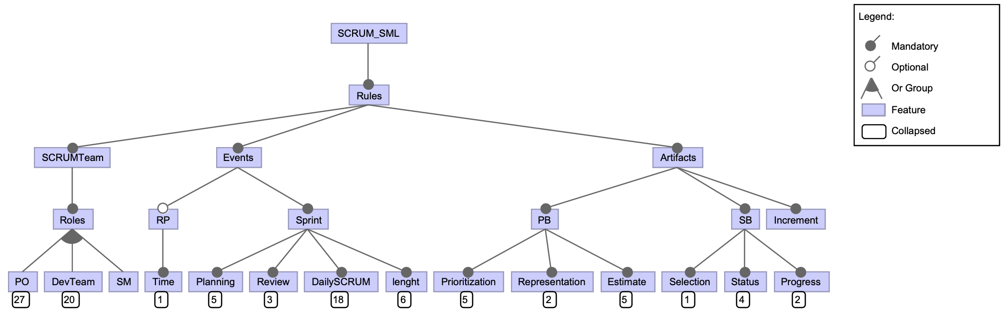
Figure 1: SCRUM Feature Model. Numbers on leaves show #constraints in that part of the model. Not shown here, for space reasons, are “cross-tree constraints” that connect choices in different sub-trees.

When human reasoning fails, often we turn to AI. Modern AI tools like the PicoSAT [Biere, 2008] solver can find millions of solutions that satisfy Figure 1. But now there is a new problem: too many solutions. So now we must ask: Q: How can we help humans choose between all the trade-offs?

Here, we explore interactive tools where human knowledge can guide the the search process. In this paper, we deliver a new state-of-the-art result by asking humans the least questions to find the most desirable solutions. More specifically, we find that a small set of easily computed “hints” can generate an approximate “partial orderings” of the candidate solutions. Using the orderings generated from those “hints”, stakeholders can guide a simple binary chop procedure to recursively prune candidates. In this way, after offering $O(\log(N))$ opinions about $N$ examples, humans can find a small set of most acceptable solutions. Hence, the answer to our question is A: Compute an approximate partial ordering, then let humans apply recursive pruning.

This paper introduces iSNEAK, a tool that tests our partial ordering approach. We show that such partial orderings are useful, even in the case of models with multiple objectives. In essence, iSNEAK is a method for controlling a large space of options with only a few samples of human knowledge. This raises certain concerns and the research questions of this paper are designed to address those concerns:

• When humans comment on small fraction of the search space does their limited knowledge means they are making sub-optimal decisions?

• Also, since human knowledge falls into a small fraction of the total space, do automated algorithm find solutions that are unacceptable to stakeholders?

Note that both these issues are really examples of one high-level problem. Specifically, can a particular kind of knowledge (algorithmic or human insight) lead to poor results? To answer this, we need two research questions that look for drawbacks with iSNEAK’s use of two kinds of knowledge (algorithmic or human insight):

RQ1: Does iSNEAK’s automatic tools generate solutions (using partial orderings) that are unacceptable to humans? To answer this question, we report on a double-blind study with a team of 20 Brazilian programmers, where iSNEAK’s results were overwhelmingly preferred over other approaches since (a) iSNEAK ran two orders of magnitude faster; (b) iSNEAK ’s attribute selection resulted in orders of magnitude fewer questions to the user; and (c) all iSNEAK ’s conclusions were more optimal than those found by other approaches.

RQ2: Does human insight (guided by iSNEAK and partial orderings) miss important solutions? To implement this check, we compare what iSNEAK finds against alternative optimization technologies, some of which explore much further than just the space of ideas understood and condoned by humans. This check explored two classes of algorithms:

• The genetic algorithms preferred by the interactive search-based SE community;

• The sequential model optimizers used by the SE configuration community.

These rival technologies, and iSNEAK were assessed using a set of 16 SE models (of size ranging up to 1000 attributes). Significantly, iSNEAK worked as well or better than anything else, even for multi-objective models with competing goals (in this work we explore models with four to five goals).

The rest of this paper is structured according to guidelines from Wohlin et al. [2012] on how to structure experiments in software engineering. As per their requirements, we first present our Methods which divide into:

• The algorithms we apply to data (in §4.1, §4.2 and §4.1) and

• The case studies used for those algorithms (see §5.3); and

• The protocol we used for human experiments (in §6.1).

The results from those methods are reported in our Results section, which is followed by a Threats to Validity section.

2 Background

In this section, we first introduce our idea of “partial orderings”. Next, we discuss the test domain where we will assess partial orderings (model-based SE).

2.1 Exploring Models via Partial Orderings

This paper argues that an efficient way to explore model optimization is partial orderings. A partial order is an ordering of a set such that, for certain pairs of elements, one precedes the other. Like any heuristic, it is not a complete inference (since there may be pairs for which neither element precedes the other, according to a partial ordering). However, as shown below, it can be remarkably effective.

A repeated result in software engineering (and other domains) [Ratner et al., 2019, Pornprasit & Tantithamthavorn, 2023, Wang et al., 2019, Nair et al., 2017] is that when optimizing for some goals, it is possible to be guided by some easy-to-compute partial heuristic. For example, automatic configuration assessment tools can be built from regression trees with just a few examples. Even if those trees become very poor predictors of performance (in an absolute sense), they can still be useful to rank (in a relative sense) different configurations. E.g., Nair, et al. used those trees to find the top 1% of configurations, even though those models had error rates as high as 90% [Nair et al., 2017]. Also, some researchers [Pornprasit & Tantithamthavorn, 2023] use generative models to improve upon supervised learning. While the results from the generative model may not be of the highest quality, all these outputs provide hints on how to better direct another algorithm (e.g., a machine learner). Further, researchers explored test case selection via crowd-sourcing since this is a fast way to collect many opinions. While the value of one opinion is questionable, they can be useful in the aggregate [Wang et al., 2019].

To say all this another way, SE researchers often guide the search for “good” solutions via some heuristic that can pre-order the space of possible solutions. To demonstrate the power of this approach, we turn to Hamlet’s probable correctness theory [Hamlet, 1987]. That theory says that the confidence of seeing an event occurring at probability $p$ after $n$ trials is $c=1-(1-p)^{n}$, which, if rearranged, tells us how many samples are required to find something:

$$n(c,p)=\frac{log(1-c)}{log(1-p)}$$ (1)

For example, to be 99.9% confident that we have found (say) the top 1% of all solutions, humans must evaluate $\approx 688$ candidates.

Now consider what happens if we can compute some partial ordering over all those solutions. For solutions sorted in that manner, Hoare’s quickselect algorithm needs only explore:

$$\begin{array}[]{rcl}\mathit{evaluations}&=&\log_{2}(n)\\ \mathit{y\mathchar 45\relax evaluations}&=&2\log_{2}(n)\end{array}$$ (2)

of the above $n$ samples. Assuming this binary chop, and repeating the above calculation, the equations say that now we only need to evaluate $\log_{2}(n=688)\approx 10$ times. If the reader finds this calculation to be over-optimistic, we point out that our experimental results in §6.2 show that iSNEAK can find good candidate solutions after just a few dozen evaluations.

One way to summarize this equation is to say that optimization problems can be easier than other tasks like classification or regression. Those other tasks require us to label examples across the entire space while optimization means looking for a small region (and pruning the rest). And that small region can be found via partial ordering.

(Aside: when discussing this work, we are often asked how this work compares to other SE researchers in what they call “partial orderings”. For example, researchers trying to reduce the state space explosion of model checking [Peled, 1998], or simplifying the number of refactoring steps for source code [Morales et al., 2018], apply a technique they call partial order reduction that prunes similar paths leading to the same result. While that work certainly shares some of the intuitions of this work, we note that (a) our partial orderings sort the entire space of solutions; after which we (b) explore $N$ solutions using $O(\log(N))$ evaluations. In this second step, what is important in our work is that our use of partial orderings lets humans guide the algorithms to their conclusions.)

The rest of this section describes model-based SE, which is the test domain used to assess the partial orderings heuristic.

2.2 Model-Based Reasoning in Software Engineering

Amorim et al. [2019] comment that model-based SE is the formalized application of modeling to support system requirements, design, analysis, verification and validation activities. Unlike document-centric approaches, models serve as blueprints for developers to write code, tools automate much of the non-creative work (which translates to gains in productivity and quality). MBSE fosters artifact reuse and product quality, while shortening time to market. They say that MBSE is part of a long-term trend towards model-centric approaches adopted by other engineering disciplines including mechanical, and electrical.

2.3 Increasing Use of Models in SE

Model-based reasoning is increasingly attractive, due to the recent increased access to cloud-based CPU farms. With that compute power, it becomes practical and simple to run many “what-if” queries on models. This means that more options can be explored before committing to one particular design. Consequently, we are seeing much more use of models in software development. The rest of this section offers some examples of that kind of reasoning.

In the realm of cyberphysical realm, it is standard practice [Chowdhury et al., 2018] to deliver hardware along with a simulation system (often written in Simulink or C). Developers then make extensive use of that simulation system during verification.

In requirements engineering, researchers [Mathew et al., 2017, van Lamsweerde, 2009] argue that building and analyzing different models helps stakeholders better understand the ramifications of their decisions. For example, software product line researchers explore a space of inter-connected features in a software design  [Mendonca et al., 2009, Chen et al., 2018, Nair et al., 2018, Galindo et al., 2019, Kira & Rendell, 1992, Hierons et al., 2016, El Yamany et al., 2014, Saber et al., 2017, Pohl et al., 2011]. Software feature models can be reversed engineering from code, then used to debate subsequent possible changes to that system [Sayyad et al., 2013a].

Proponents of domain-specific languages argue for a systems-development life-cycle that begins with (a) defining a domain language [Fowler, 2010], then (b) modeling & executing that system via that language. Low code proponents then add some visual editor to allow for rapid changes to the model [Prinz et al., 2021]).

Safety critical researchers often build (or generate) two models: one to represent the system under study and another to represent the safety properties. Automatic tools then look for violations of the safety properties within the systems model; see  [Holzmann, 2014, Backes et al., 2019].

Models can be used for the generation of runtime systems. This is especially useful for automotive and embedded systems that make extensive use of models (e.g. generating executables from Simulink [mader2013oasis]).

There is now an increased awareness that any software system is a combination of services that can be refactored and packaged separately, or together on some new platform. As more and more monolithic ”on-premise” systems are refactored and reconfigured for the cloud, we have learned that it is important to model the parts of our software and how each part can connect to other parts [Yedida et al., 2023, 2021].

Researchers in search-based software engineering (SBSE) make extensive use of executable models. In this work, there is some set of goals to be achieved, which may be competing, and a model that comments on how domain decisions effect those goals. SBSE is often treated as an optimization problem where some optimization explores all the nuanced way decisions allow us to trade-off competing goals. In our own work, we have applied SBSE to models of cloud-based architectures [Chen & Menzies, 2018] (looking for ways to reduce the cost of the overall design); NASA spaceships [Feather & Menzies, 2002] (looking for cheaper satellites that can handle more error conditions); video encoders [Nair et al., 2018] (looking for better and faster compression control parameters); software process models [Sayyad et al., 2013b] (looking for ways to deliver more functionality, with less cost)

2.4 Why We Need Better Model-based Reasoning

Better model-based reasoning in SE is becoming a legislative necessity. Green [2022] reports on policies demanding humans-in-the-loop auditing of decisions made by software. When faced with large and complex problems, cognitive theory [Simon, 1956] tells us humans use heuristic “cues” to lead them to the most important parts of a model before moving on to their next task. Such cues are essential if humans are to reason about large problems. That said, using cues can introduce their own errors: …people (including experts) are susceptible to “automation bias” (involving) omission errors—failing to take action because the automated system did not provide an alert—and commission error [Green, 2022]. This means that oversight can lead to the opposite desired effect by “legitimizing the use of faulty and controversial (models) without addressing (their fundamental issues”) [Green, 2022].

2.5 Models: Detailed Examples

As an example of the prevalence of SE models, later in this paper, we offer details on the 16 models used in this study. While full details on those models are available in §5.3, the rest of this section offers some summary notes such as the problem solved by each model.

The OSP2 model (for “orbital space plane, version2”) describes the software context of a second generation NASA space plane. Expressed in the terminology of Boehm’s COCOMO system [Boehm et al., 1995], OSP2 lists the range of acceptable software reliability (it must be very high), database size (which is variable), developer experience (which can be changed by management assigning difference developers to the project), and so on. The problem solved by OSP2+iSNEAK is to “generate good management recommendations” that satisfy the constraints of that project, while also minimizing the development time (as judged by the COCOMO model) while also avoing other factors that increase the risk of cost overrun (as judged by other Boehm models).

GROUND, FLIGHT are similar to OSP2, but represent two specialized classes of NASA software (flight software and ground software). The problem solved by these two models are the same as OSP2 (but for special kind of specific software types).

While OSP2,GROUND,FLIGHT assume waterfall style development, the POM3 model concerns itself with agile projects. This paper explores three POM variants:

• POM3a representing a very broad space of projects; and

• POM3b representing safety critical small projects; and

• POM3c representing highly dynamic large projects.

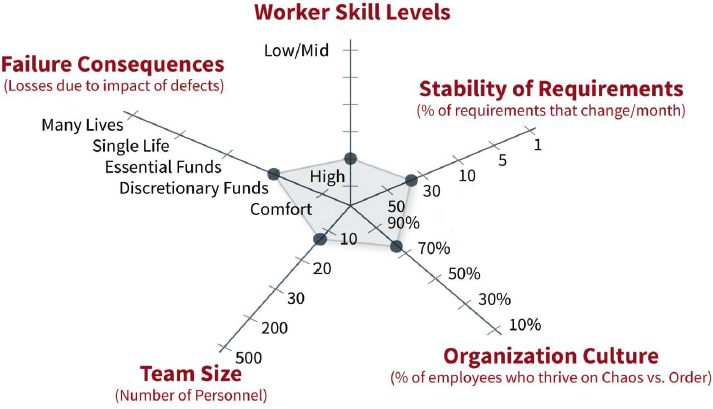
Figure 2: According to Boehm and Turner [Boehm & Turner, 2003a], agile is best suited for projects in the middle of this figure.

The problem solved by the POM3+iSNEAK model is deciding “what tasks to complete in the next sprint?” (where a sprint is a very short period of intense coding with the aim to produce some specific deliverables). POM3 adjusts those choices using knowledge of contextual factors associated with the development project (see Figure 2). These contextual factors were identified by Boehm and Turner’s in their text: ”Balancing Agility and Discipline: A Guide for the Perplexed”’ [Boehm & Turner, 2003a]. Note that while the problems solved by POM3* are all the same, the solutions found are tuned to the different kinds of software represented in those different models.

For all these POM models, the goal is to maximize the number of requirements meet while minimizing the time to completion and idle time (time spent waiting for some other team to complete some required module).

The rest of our models come from the software product line research. Here, a large space of potential software projects are modeled as a tree of features (and super-features are meet via some conjunction/disjunction of sub-trees). Between the tree, there may be “cross-tree constraints”; i.e. things that must be absent or present in one branch to enable a feature in another branch. From one product line, many software designs can be generated, provided that each satisfy the cross-tree constraints. When combined with some optimizing technology like iSNEAK, the problem solved by these models plus iSNEAK is “what product to build?”. To answer that question, an optimizer must trade off between competing goals such as minimizing development time and maximizing number of features delivered. An example software product line was the SCRUM model shown in Figure 1. Another software product line model used in this paper represents options with a BILLING system. Apart from that, this paper will also optimize eight other artificially generated SPL models of increasing size and/or frequency of cross-tree constraints.

We note that model-based reasoning is a victim of its own success. Now that we can build and execute many models, those models can produce too many different solutions. Hence, as stated in our introduction, the problem now becomes “how to understand everything the models are telling us?”. Hence, this paper.

2.6 Why Not Explore Models Using Traditional Optimization Methods?

This paper is about optimization. Optimization problems, like those discussed in our introduction, have been well-studied for decades in the operations research literature [Winston, 2022]. There are many reasons to be cautious about using traditional optimizers for model-based SE. Those optimizers often assume continuous functions with numeric attributes that can be differentiated at all points along a function (differentiability is a key requirement for any classical gradient descent algorithm). Models like Figure 1, on the other hand, have many non-numeric attributes and are not expressed in the equational form needed by traditional optimizers.

Also, traditional optimizers may make unrealistic assumptions about the nature of model goals. Researchers like Harman [Harman & Jones, 2001] note that SE often requires trading off between competing many goals and, in that context, there may not be a single optimal but rather a (small) space of most acceptable solutions which must be debated by stakeholders.

Further, if used “off-the-shelf”, traditional optimizers can waste much time exploring issues that many humans find irrelevant or incomprehensible. While models may contain many variables, any one subject matter expert may only have experience with a small number of them. One result from the user study of this paper is that when stakeholders are asked to comment on all model attributes (e.g., the 128 attributes of Figure 1), they only ever comment on around 20 attributes. This means that, in our experiments on Figure 1, the space where their expertise can be applied is just $\ 2^{20}/2^{128}\approx 10^{-33}$ of the total state space. Hence we seek methods that that can respond well to very small samples of human insight.

3 Our Proposal: The iSNEAK Algorithm

As stated in our introduction, the idea of this paper is a few quick “hints” can let us quickly generate a partial ordering of candidate solutions, which can then be pruned using some $O\log(n)$ variant of a binary chop algorithm.

SWAY sorts candidates via a recursive binary chop inspired by Chen et al.’s SWAY algorithm [Chen et al., 2018]. SWAY recursively evaluated two very distant points east,west, then recurses on the half associated with the “better” of east or west (where “better” is a domination predicate, discussed below).

This algorithm runs on discretized attributes. To discretize numerics, following the advice of Kerber [1992], numbers are initially divided into 16 ranges equal-width bins. Then, while we can find two “mergable” adjacent ranges $r_{1},r_{2}$, we combine them into the range $r_{12}$. “Mergeable” means that the standard deviation of the merged ranges is less than or equal the expected value of the standard deviation of parts. For ranges with $n_{1},n_{2}$ examples, this is:

$$\sigma_{r_{12}}\leq(n_{1}\sigma_{r_{1}}+n_{2}\sigma_{r_{2}})/(n_{1}+n_{2})$$

After that, Chen et al.’s boolean distance metric [Chen et al., 2018] is used to measure the distance between two candidates (as a function of the number of overlapping ranges). With that distance metrics, the two remote points east,west can be found in linear time, using the Faloutsos [Faloutsos & Lin, 1995] heuristic. Formally, this process of clustering via two distance points is defined as a recursive FASTMAP algorithm [Faloutsos & Lin, 1995] which belongs to the Nyström  [Platt, 2004] family of PCA approximations:

• Let $E$ (east) and $W$ (west) be seperated by distance $c$.

• Let $a,b$ be the distance of some example to $E,W$.

• All other examples have distances $a,b$ to $E,W$, respectively and distance $x=(a^{2}+c^{2}-b^{2})/(2ac)$ on a line drawn $E$ to $W$.

• To halve the data, split on the median $x$ value.

When recursively processing $N$ candidates, SWAY halts when it reaches $n=\sqrt{N}$ examples. This stopping threshold was selected based on advice from Webb et al. [Yang & Webb, 2009] on how best to divide data.

SWAY only sorts candidates by the goal attributes used in the Zitzler predicate of Equation 3 (described later in this paper). Hence, SWAY selects solutions that may not fall into the region understood and condoned by humans. To fix SWAY, we note that models have two kinds of attributes:

• Goal attributes such as cost and defects. For example, Figure 1 has the four-goal attributes listed in the introduction.

• Independent attributes like choice of programming language. For example, Figure 1 has 128 independent attributes.

In our experience, when faced with models like Figure 1, humans often have opinions about many of the independent attributes (e.g., SCRUM developers might prefer interactive languages like Python over languages that need a slow batch compile, like “C”).

iSNEAK attempts to repair SWAY as follows. Whereas SWAY prunes based on the goal attributes, iSNEAK mostly uses the independent attributes to find a small set of short questions that sorts then prunes, candidates. The core of iSNEAK is (a) a recursive clustering algorithm that creates a binary tree of clusters and (b) a attribute selection algorithm that reports what is the smallest set of ranges that most distinguishes between sibling sub-trees. To prune a binary tree of clusters, iSNEAK repeatedly looks for the largest sub-trees that can be most distinguished by the fewest independent attributes. Readers familiar with the ML literature will recognize our use of the INFO-GAIN entropy-based attribute selector [Hall & Holmes, 2003]. We use this attribute selector since our current results suggest that it is remarkably effective (but in future work, we plan to explore other attribute selectors).

Here are the full details on the iSNEAK algorithm:

1. iSNEAK’s starts with $N$ unevaluated candidates.

2. iSNEAK uses SWAY’s recursive FASTMAP clustering, but now, after labeling candidates according to the distance to two remote east,west points, iSNEAK then forks two branches for all the candidates nearest to either east or west. To say that another way, while SWAY always prunes one of these branches, iSNEAK always explores both branches.

3. In the tree of clusters generated by iSNEAK, each subtree has two sibling branches. iSNEAK calculates $e_{1},e_{2}$ being the sum of the entropy in the two branches, as well as $e_{0}$ which is the same calculation over both branches.

4. iSNEAK sorts subtrees by $S{\times}(e_{0}-e_{1}){\times}(e_{0}-e_{2})$ where $S$ is the number of candidates in a subtree and $(e_{0}-e_{i})$ is the reduction in entropy seen after selecting the $e_{i}$ branch (and pruning the other). The subtree with largest $S{\times}(e_{0}-e_{1}){\times}(e_{0}-e_{2})$ is the one where we can best prune the most candidates. For this sub-tree, we apply INFO-GAIN to find up to six attributes that most distinguish the branches. We then ask the stakeholder to select their preferred ranges in those selected attributes.

5. To decide which of the branches we should prune, we select at random one candidate from each branch. For those example we calculate their y-evaluation score to generate goals $g_{1},..g_{G}$. We then add a new goal $g_{G+1}$ which is the ratio of preferred ranges in that example. Using the Zitzler formula of Equation 3 (described later in this paper), we then select the example with the “better” goals $g_{1},..g_{G},g_{G+1}$ (and here, ask Zitzler to try maximizing $g_{G+1}$).

6. If $\sqrt{N}$ candidates remain, then exit. Else, we loop to step 3.

After iSNEAK finds $\sqrt{N}$ candidates, these are passed to SWAY which then returns $\sqrt{\sqrt{N}}$ best candidates that are within the approved range of options for an oracle.

4 Alternatives to iSNEAK

In order to assess iSNEAK, this section (and the next) describe rival technologies that have been applied to many-goal model-based reasoning in SE:

• Genetic algorithms, used for interactive search-based SE;

• Sequential model optimizers, used for SE configuration.

4.1 SBSE and Interactive search-based SE

Search-based SE methods explore design trade-offs using evolutionary programs that work in generations $G_{i}$ of examples:

1. Generation $G_{0}$ is the initial population.

2. Each new generation $G_{i+1}$ is built by

   1. Randomly mutating the $G_{i}$ solutions,

   2. Then selecting the best individuals,

   3. y-evaluating these individuals

   4. Then mixing together (also known as crossover) parts of two best individuals to create a new example for $G_{i+1}$

This kind of reasoning must assess and compare solutions (in step 2b of the above). In single-objective optimization problems, a simple sorting function can rank goals between candidates. However, when dealing with many-objective reasoning, candidates must be ranked across many goals. As the number of goals increases, simple schemes such as boolean domination find it harder to distinguish different candidates. Following Sayyad et al. [2013c]’s advice we use Zitzler’s continuous domination predicate [Zitzler & Künzli, 2004] to rank candidate solutions in order to evaluate the effectiveness of our algorithms. This predicate favors $a$ over $b$ model if jumping from $a$ “loses” most:

$$\begin{array}[]{rcl}\textit{worse}(a,b)&=&\textit{loss}(A,B)>\textit{loss}(a,b)\\ \textit{loss}(a,b)&=&\sum_{j=1}^{n}-e^{\Delta(j,a,b,n)}/n\\ \Delta(j,a,y,n)&=&w_{j}(y_{j}^{a}-y_{j}^{b})/n\end{array}$$ (3)

where “$n$” is the number of objectives and $w_{j}\in\{-1,1\}$ depending on whether we seek to maximize goal $x_{j}$ and $o_{j,A},o_{j,B}$ are the scores seen for objective $o_{j}$ for $A,B$, respectively.

Interactive SBSE (iSBSE) is a variant of SBSE that tries to include humans in the reasoning process. One drawback with these iSBSE tools is cognitive fatigue. Typical control policies for genetic algorithms are to 100 individuals in $G_{0}$, which are then mutated for a hundred generations [Holland, 1992]. Most stakeholders can only accurately evaluate a small fraction of the 100*100=10,000 individuals generated in this way.

To reduce cognitive fatigue, iSBSE researchers augment genetic algorithms with tools that enable pruning the search space, without having to ask the stakeholders too many questions. For example, Palma et al. [2011] use a constraint solver (the MAX-SMT algorithm) to evaluate pair-wise comparisons of partial model solutions to decrease their search space. We do not compare iSNEAK against this method since their technique has scaling problems:

• Their biggest model had 50 variable constraints.

• iSNEAK, on the other hand, has been successfully applied to a 1000 variable model: see §6.2.

In other work, Lin et al. [2016]’s iSBSE code refactoring tool calculates and recommends refactoring “paths” from the starting point to the target with each path being a sequence of atomic refactorings. Then, stakeholders interactively examines the recommended steps to accept, reject, or ignore them. These interactions will then be used as feedback to calculate the next recommendation. But like Palma et al., Lin et al. did not demonstrate that their methods can scale to the same size models as we process later in this paper.

In yet other work, Araújo et al. [2017] combined an interactive genetic algorithm with a machine learner. Initially, humans are utilized to evaluate examples, but once there are enough examples to train a surrogate; i.e., a model learned via machine learner that can comment on solutions, this surrogate starts answering queries without having to trouble the stakeholders.

THe Araújo et al. tool is a useful candidate for comparative studies with iSNEAK. Their inputs representations could be readily adapted to our models. Also, they recommended exploring software product lines such as Figure 1 as future work. Accordingly, the study compares iSNEAK against Araújo et al.

1. SAMPLE: From $N$ examples, a small sample of $m$ candidate solutions are y-evaluated. 2. GENERALIZE: Using the sample of $m$ y-evaluated solutions, a surrogate is built via machine learning. 3. EXPLORE: The surrogate make guesses about the remaining $N-m$ number of non y-evaluated candidates. 4. ACQUIRE: The “most interesting” guess (as determined by an acquisition function is then y-evaluated. 5. LOOP: $m=m+1$; Exit if $m>\mathit{budget}$. Else goto step 2.

Table 1: Sequential Model-Based Optimization: general framework. Step 4 of Table 2 shows a specific acquisition function.

4.2 Sequential Model-Based Optimization

Recall that Araújo et al. reduced the number of questions to the stakeholders by building a surrogate. Once that surrogate is available then when new solutions are generated, these are evaluated by the surrogate (without having to ask the stakeholders any questions).

1. SAMPLE: From $N$ examples, a sample of $m_{0}=60$ candidate solutions are y-evaluated. 2. GENERALIZE: Using the sample of $m$ evaluated solutions, a regression tree is built by CART [Leo Breiman, 1984], one tree per model objective. 3. EXPLORE: These CART models make guesses about the remaining $N-m$ non y-evaluated candidates. 4. ACQUIRE: In FLASH, the “most interesting” guess is the one that has maximum objective values across $n$ random projections. (a) Each non-y-evaluated candidate has $G$ goals $(g_{1},g_{2}..,g_{G})$ (computed by the CART model learned in step 2). FLASH normalizes all these goals 0..1 for min..max. (b) Each non-y-evaluated candidate has $G$ weights $(w_{1},w_{2},...w_{G})$ where $w_{i}=(-1,1)$ for goals being minimized or maximized (respectively); (c) Each non-y-evaluated candidate’s goals is multiplied by a set of $G$ random weights $(r_{1},r_{2},..r_{G})$ where $0\leq r_{i}\leq 1$. (d) The most interesting non y-evaluated candidate has max $\frac{1}{N-m}\sum_{i}^{G}g_{i}{\times}w_{i}{\times}r_{i}$ 5. LOOP: $m=m+1$; Exit if $m>(\mathit{budget}=120)$. Else goto step 2.

Table 2: A variant of SMBO, as seen in FLASH [Nair et al., 2018]. FLASH’s use of random projections (in step 4c) was inspired by earlier work on the MOEA/D algorithm [Zhang & Li, 2007]. The control parameters shown in this figure ($m_{0}=60,\mathit{budget}=120$) come from prior work [Nair et al., 2018].

The use of surrogates is an important technique in the automatic configuration literature. Traditional configuration methods require the evaluation of many candidates. For example, in 2013, Apel et al. proposed the use of the CART regression tree learner to generate a model from some historical examples that could be used to assess configuration options for future configuration problems [Guo et al., 2013]. That said, literature reviews in this field such as Ochoa et al. [2018] lament the narrow range of algorithms used in this area. Firstly many of these tools still require a large number of pre-evaluated candidates. Secondly, the configuration tools reported by Ochoa et.al. (that reportedly supposedly support human interaction), often use a human ranking of attributes that is fixed for all candidates [Ochoa et al., 2018]. Hence those reportedly interactive tools can overlook nuances related to specific examples.

Nair et al. use surrogates in a differfent way. In their tool, new examples are assessed on a case-by-case basis by sequential model-based optimization [Hutter et al., 2011, Zuluaga et al., 2013] (SMBO). Table 1 shows their acquisition function loop that uses the surrogate to guess which candidate should be reviewed next.

Acquisition functions are the core of tools that use SMBO. While working on automatic software configuration, Nair et al. explored several acquisition functions [Nair et al., 2018]. For SE models, they found that standard SMBO methods (using Gaussian Process Models) did not scale very well. Instead, they found that regression tree models based on CART [Leo Breiman, 1984] scaled up to the kinds of large models seen in SE. Following their recommendations, this paper will use their FLASH sequential model optimizer, described in Table 2. Note step 4d, where one new example is evaluated. This is the point where some oracle would be asked for their opinion on a candidate (e.g., some human could be asked a question or some model could be executed to obtain y-values).

5 Methods

5.1 Generating Candidates

Chen et al. [2018] found that if they generated very large initial populations (e.g., 10,000 candidates), then their recursive binary chop could very quickly find solutions as good, or better, as genetic algorithms that take an initial population of (say) 100 candidates then mutate them over 100 generations. Following their advice, iSNEAK uses various mechanisms to generate those 10,000 candidates:

• For models expressed that can be expressed as logical constraints (e.g., software product lines like Figure 1) candidate solutions were generated via PicoSAT v0.6.3.

• Our other models (specifically XOMO and POM3 variants) came with their own procedural engine for generating examples.

5.2 Source Code for Rival Algorithms

Arcuri et al. [Arcuri & Briand, 2011] recommend that algorithms need to be compared against some simple baseline. For that purpose, we use a Non-Interactive Genetic Algorithm (NGA) which is the same genetic algorithm used by Araújo et al. but without human interactions. This approach serves as a baseline for comparison towards answering our second research question, where we only perform y-evaluations to optimize our models. For the population control parameters of NGA, we used the advice of Holland et al. [Holland, 1992]; i.e., 100 valid candidates and is run for 100 generations, thus generating 100 new candidates each time. As to the cross-over and mutation method, we retained the Araújo et al. settings; i.e., 90% crossover and a mutation rate set to $1/A$ (where $A$ is the number of attributes in that model).

iSNEAK is also compared to a state-of-the-art evolutionary method; specifically, FLASH [Nair et al., 2018] and the Araújo et al. iSBSE [Araújo et al., 2017] algorithm We choose their algorithms for their recency and superior performance (compared to other methods in their field [Zuluaga et al., 2013]). Also, the Araújo et al. [2017] algorithm, on the other hand, is engineered to accept a wide range of models as input.

The code for FLASH, written in Python, comes from the Nair et al. repository. Araújo et al. did not offer a reproduction package for their work so we reimplemented their code from their descriptions.

5.3 Case Studies: Models Used in this Study

Table 3 offers statistics on all the models used in this study.

The models POM3A, POM3B, POM3C, OSP2, FLIGHT and GROUND are small and have no constraints (so all solutions generated to these models are valid). All the other models are much larger and have many constraints that only 1% to 3% of the solution space is valid.

OSP2, GROUND and FLIGHT are variants of XOMO [Menzies & Richardson, 2005] which combine four different COCOMO-like software process models in order to calculate metrics for project’s success. The XOMO model, is a general framework for Monte Carlo simulations that combine four COCOMO-like software process models from Boehm’s group at the University of California. Containing between 6 and 12 variables on each of it’s variants, the XOMO model is a representation of real situations in a software project. Under this model, a user can obtain four objective scores: (1) project risk; (2) development effort; (3) predicted defects; (4) total time for development. The model was developed with data collected from hundreds of commercial and Defense Department projects [Boehm & Turner, 2003b]. As to its risk model, it is defined as a rule based algorithm on certain variables on these models associated with risk (e.g.: demanding more reliability whilst decreasing analyst capability). As such XOMO measures risk as the percent of triggered rules

	“Free” variables	Constraint	Number
	(i.e., values that can be adjusted).	ratio	of goals
OSP2	6	0	5
POM3A	9	0	4
POM3B	9	0	4
POM3C	9	0	4
FLIGHT	11	0	5
GROUND	12	0	5
BILLING	88	1.02	4
125FEAT	125	0.25	4
SCRUM	128	0.97	4
250FEAT	250	0.25	4
.25 C.D.	500	0.25	4
.50 C.D.	500	0.50	4
.75 C.D.	500	0.75	4
1.00 C.D.	500	1.00	4
500FEAT	500	0.25	4
1000FEAT	1000	0.25	4

Table 3: Number of variables being optimized and constraint ratio. For the models on the first few rows, the constraint ratio is zero (since every solution from those models is valid). For the other models, the constraint ratio is the number of constraints per clause.

POM3A, POM3B, and POM3C are variants of POM3 with increasing complexity (where “complexity” is measured as the number of constraints per variable). POM3 in general is a model for exploring the management process of agile development [Boehm & Turner, 2003b, a, Port et al., 2008]. The objective of POM3 is to find an effective configuration of its attributes in order to achieve better project success metrics, also being a many-goal problem. POM3 simulates the Boehm & Turner [2003b] model of agile programming, where teams select tasks as they appear in the scrum backlog. The idea of this model is to design a better management process for agile development that seeks to: (1) increase completion rates; (2) reduce idle rates; (3) reduce overall cost.

The BILLING and SCRUM models were obtained from the SXFM SPLOT-Research web site. In these software product line models, we seek to minimize costs, efforts, and predicted defects while maximizing features associated with previous success.

The SCRUM model of Fig. 1 is a software product line model defining the possible legal configurations of the SCRUM organizational framework. BILLING is a software product line model containing valid configurations for a billing software system. In both models, due to their constraints, less than 2% of its configurations are valid.

The SPLOT website has a tool for artificially generating models. This tool is useful for stress testing an algorithm by e.g., generating models of increasing complexity. We used eight such models:

• We increased features size while using the same ratio of constraints to features for 125FEAT, 250FEAT, 500FEAT. 1000FEAT.

• In 0.25 C.D, 0.75 C.D, 0.50 C.D and 1.00 C.D, the number of features was kept constant (at 500) while the ratio of constraints to features was increased.

These last ten models were taken from the SXFM format and converted into the Dimacs format using FeatureIDE [Kastner et al., 2009]. And from the Dimacs format, we use a PicoSAT to generate a database of valid solutions for each.

5.4 Manual and Automatic Oracles

We conducted two studies:

• Human-in-the-loop, to see if human trust or accept our solutions.

• Fully automated, to test dozens of models.

In the former, humans were the oracle. In the latter, each attribute was given a randomly assigned priority (and approved answers where those using attributes that maximized the sum of that priority).

5.5 Evaluation Metrics (distance to heaven)

To evaluate the optimally of solutions found by different methods, we must see where our solutions fall within the space of all solutions. To that end we:

• Ran one method (NGA, iSBSE, FLASH, etc) to collect a small number of recommended candidates.

• Evaluated and Y-Evaluated all candidates and ranked them all;

• Find the recommended candidates ranks within all candidates.

For ranking all candidates, using the Ziztler predicate, we can obtain a vector Z containing all candidates sorted from best to worst. The “distance to heaven” of a specific recommended candidate, denoted $x$ by its index $i_{x}$ within $Z$ as follows:

$$\mathit{d2h}_{x}=i_{x}/|Z|$$ (4)

Note that this number ranges from 0 to 1 and solutions with lower numbers are better (since they are closest to heaven).

6 Experimental Results

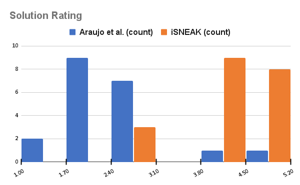
Figure 3: RQ1 results. Distribution of ratings given by human experts to presented solutions. The x-axis denotes human ratings and the y-axis shows the frequency counts by which humans offered those ratings.

6.1 RQ1: Does iSNEAK’s automatic approach generate solutions that are unacceptable to humans?

RQ1 addresses the core issue that motivated this paper; i.e., how can we make AI deliver solutions that humans agree with? As mentioned in §1, stakeholders may have preferences for a tiny fraction of the total space. Hence, it is possible that automated tools like iSNEAK will differ from what a stakeholder considers acceptable. RQ1 tests for the presence of that problem.

The RQ1 experiment was performed in accordance with the Investigator Review Board policies of the North Carolina State University. Note that in the following experiments, human input is used in all the comparison algorithms studied here (i.e., both iSNEAK and Araújo et al.) Within the experiment, we only asked humans to compare iSNEAK with the iSBSE method proposed by Araújo et al. Neither FLASH nor NGA was used here. We make this choice for two reasons:

• Every added component to a human-in-the-loop study increases the effort associated with our human subjects. Hence we were keen to minimize their cognitive load.

• Secondly, FLASH and the NGA behaved so poorly in our automatic trials that there was no pressing need to test them in RQ1.

To obtain human subjects, we reached out to our contacts in the Brazilian I.T. community where one manager granted us access to 20 of her developers, on the condition we took no more than two hours of their time (for initial briefing and running the experiments). Our choice of subjects lead to certain decisions for our experimental design. We had to use a model with attributes that our subjects understood. In consultation with the manager, we reviewed several models (before speaking to subjects) and the decision was that POM3a was the most approachable for our subjects.

For this experiment, subjects were selected by their manager. All subjects had at least 4 years of experience in the field and 3 years of experience in an agile team. Subjects were made aware that the manager endorsed their participation in this study. No added incentives were offered to subjects except a commitment that if in the future they wanted to use the tool, we would make it freely available and support their use. Subjects and their specific results were guaranteed anonymity from their manager. Thus, the experiment did not collect logins, names, or IP addresses.

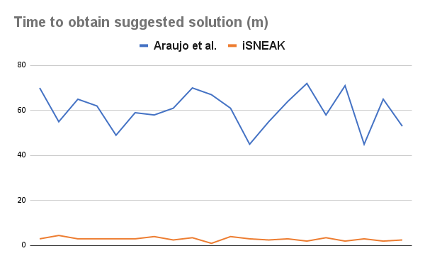
Figure 4: RQ1 results: Human effort required for each solution, in minutes

Prior to collecting data, we ran a short (under 20 minutes) in-person meeting with all participants (including the manager of that group, who also worked as a subject). Subjects were introduced to the goals of the work and briefed on the models. After that, subjects had 1.5 hours to complete the experiment during which time, they were asked not to talk to each other about their experiences. During the experiment, subjects were silently observed in a company office by one of the authors. Subjects installed and ran our software locally on their own machines. At the end of the experiment, subjects rated two configurations (using a score of 0 to 5, 0 being the worst).

In order to control for experimental-subject bias, after running both the Araújo et al.’s tool and iSNEAK tools, the two obtained solutions were presented in a randomized order (so that the iSNEAK solutions did not always appear in the same place on the screen). This meant that our subjects never knew from which tool came each solution they were asked to evaluate at the end.

As seen in Fig. 3, our subjects strongly preferred iSNEAK. The median score for iSNEAK’s solutions was 4 while the median score for Araújo et al.’s solutions was 2. Hence for RQ1, we say: For models we could show to our subjects in their available time, SNEAK’s solutions are acceptable.

We have recorded the time it took each participant to obtain a solution with each tool. As seen in Fig. 4, iSNEAK requires orders of magnitude less human time in order to obtain preferable solutions.

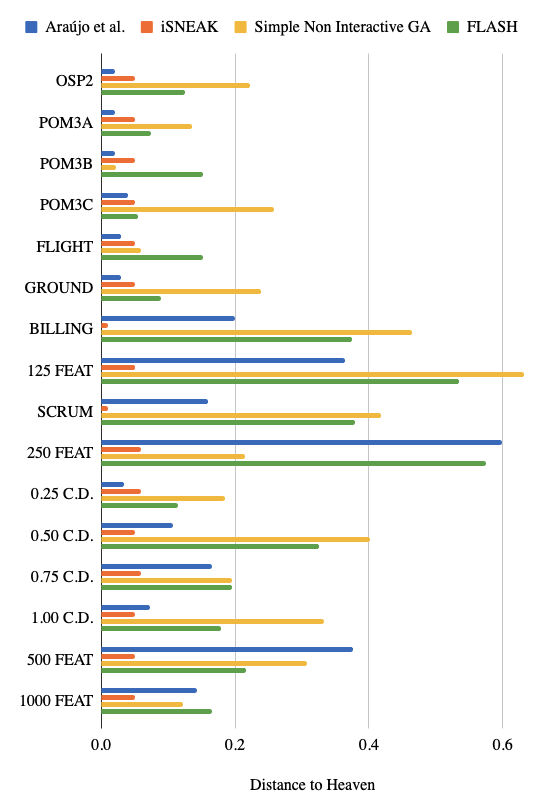
Figure 5: RQ2 results. Median d2h values seen over 20 runs (Log scale on the Y axis). For a definition of d2h, see Equation 4 in §5.4. Note that lower values are better.

6.2 RQ2: Does human insight (guided by iSNEAK and partial orderings) miss important solutions?

RQ2 addresses the following question: are human opinions detrimental to optimization, or, if we generate solutions using the methods of RQ1, will we achieve sub-optimal results?

To answer this question, we explore numerous models other than the POM3a model used for RQ1. To facilitate this process, we used some oracle that can comment on 320 results; i.e., 20 repeats over 16 models (many of which are unfamiliar to specific subject matter experts). Hence we needed to build an automatic oracle.

To do this, before any interaction in each run, our oracle would randomly assign priority values for all of the model’s variables. Then using those priority values it would be able to consistently respond to any oracle questions posed by our algorithms. These priority values are set according to a random seed.

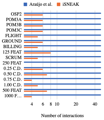
Figure 6: RQ2 results. Any iSBSE tool will, $I$ times, ask a stakeholder about $S$ attribute. Shown here are the $I,S$ numbers seen in 20 runs (different random number seeds each time).

Fig. 6a : Number of interactions $I$ (medians from 20 runs). Here, lower values are better. Note that the blue bars have a fixed top value since that parameter is hard-wired into the Araújo et al. architecture.

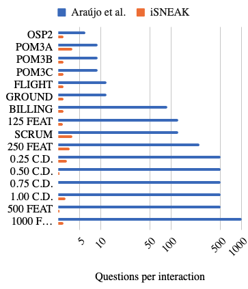
Fig. 6b: Median questions $S$ (in 20 repeats) asked per interaction. Here, lower values are better.

All results come from 20 repeated runs (with different random number seeds) of an automatic oracle exploration of our models.

Fig. 5 comments on the effectiveness of iSNEAK’s questions. Usually, iSNEAK can find results within 2% to 3% of the best solution ever seen for a model. More specifically, in Fig. 5:

• For all models, the simple GA usually performs worst.

• FLASH always ranks third or fourth best.

• Araújo et al.’s tools have medians better than iSNEAK for
  unconstrained models (the first 6 models). But for models with constraints (i.e., from BILLING downwards), iSNEAK out-performs Araújo et al. Sometimes, those wins are very significant: e.g., see BILLING here iSNEAK’s median d2h scores are an order of magnitude better than the other algorithms.

• When iSNEAK lost to Araújo et al., the difference is usually very small (the actual d2h performance deltas from the best results are $\{1,2,2,3,3,3\}\%$).

Fig. 6a shows that when Araújo et al. y-evaluates its 10,000 candidates, it pauses around 50 times to ask stakeholders some questions. As shown in Fig. 6b, these questions cover all the attributes in the model, which means the size of the interaction for Araújo et al. scales linearly with the number of variables in the model. On the other hand, iSNEAK pauses around 20 times, and when it does, it asks far fewer questions, and as seen in Fig. 6b the size of iSNEAK’s interactions has no direct relationship with the size of the model.

Just to clarify, the reason Araújo et al. asks more questions than iSNEAK is that when Araújo et al., ask the stakeholders questions, those questions mention every attribute in the model (e.g., all 128 attributes of Figure 1). On the other hand, before iSNEAK asks a question, it applies the attribute selection methods of §3 in order to isolate the most informative attributes.

We answer RQ2 as follows: For large and complex models with many constraints, iSNEAK is the clear winner (of the systems studied here). To be clear, sometimes iSNEAK is defeated by other methods– but only by a very small amount and only in simple models (that are both very small and have no constraints). More importantly, measured by the human cost to find a solution, iSNEAK is clearly the preferred method. We say cost is number of interactions times number of questions per interaction. Using Fig. 5, we compare the cost for our different systems. iSNEAK’s oracle cost was 1%,4% of Araújo et al. for the constrained and unconstrained models

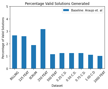
Figure 7: Valid Solutions over 20 runs (Technical aside: to handle these invalid solutions, we added a post-processor to the Araújo et al. algorithm that rejected invalid solutions.)

6.3 Other Issues

We have other reasons to recommend iSNEAK over the methods of Araújo et al.: 100% of all the solutions explored by iSNEAK are valid. The reason for this is simple: we let PicoSAT, or the model generative tool, generate valid solutions, then we down-sample from that space. Genetic algorithms, on the hand, such as those used in Araújo et al. mutate examples without consideration of the logical constraints of a domain.

This is a significant and important aspect of iSNEAK. Fig. 7 showed what happens when we take the solutions generated by Araújo et al.’s genetic algorithm [Araújo et al., 2017] for the SPL models, then applied the model constraints to those solutions. As seen in that figure, most of the solutions generated by their methods are not valid. This also applies to NGA and FLASH, which waste most of their time evaluating invalid solutions.

7 Discussion

7.1 Threats to Validity

As with any empirical study, biases can affect the final results. Therefore, any conclusions made from this work must be considered with the following issues in mind.

Evaluation Bias - In our RQ1 experiments, we studied 20 software engineers using iSNEAK to select for a good POM3A [Boehm & Turner, 2003b, a, Port et al., 2008] solution (a model for exploring the management process of agile development). Although the number of professionals could be higher to provide us with a more reliable evaluation of the approach, we have mitigated this by selecting only professionals with at least 4 years of experience in the field and 3 years of experience in being in an agile team.

Sampling Bias - This threatens any empirical study using datasets. i.e, what works here may not work everywhere. For example, we have applied iSNEAK to two real-life models of different software product lines, six XOMO and POM3 models, and eight artificially generated feature models of varying characteristics (see §5.3). But, the behavior of iSNEAK on significantly larger models (i.e., hundreds of thousands of attributes) still needs to be evaluated.

Another concern is that if the models studied here are “trivial” in some sense, then there may be very little value added by iSNEAK. We believe these these models are not trivial for several reasons. In fact, for all practical purposes, these models have a search space so large that it cannot be enumerated. Consider, for example, the SCRUM model with its 128 binary options. From Figure 7, we see that (usually) 98% of thee randomly generated solutions might violate domain constraints. That still leaves a space for at least $2^{128}*0.02=10^{38}$ solutions. In our experience with PicoSAT, it takes 12 hours to generate 100 million solutions. Hence $2^{128}*0.02$ solutions would require nearly $10^{26}$ years to enumerate.

Algorithm bias Our reasons for using the the Araújo et al. [2017] algorithm were described in §4.1, but future work needs to explore other algorithms. There are many other state-of-the-art optimizers such as OPTUNA [Akiba et al., 2019] and HYPEROPT [Bergstra et al., 2013] and many more aside.

7.2 Related Work

The connection of this work to other optimization methods was discussed above. As to the connection of this work to our prior work, this paper extends work by Chen, Menzies et al. on fully automatic methods for exploring models [Chen et al., 2018] via recursive random projections. Here, we change that search method such that some oracle can interject themselves at each level of the recursion. This is very significant change. Before, the reasoning was some black-box approach that cannot be guided by human preference. Now, we can show that humans+AI can work together to find good solutions with very little effort.

As to our own prior work with iSNEAK, in an unpublished draft, we applied an earlier version of this algorithm to the problem of learning from very small data sets. This paper differs from that prior work in several significant ways. Firstly, that article lacked any facility for human-in-the-loop interaction. But here, as discussed in §5.4, we exploit that facility in two important ways:

• In one of our studies, we ask humans for their opinions during the optimization process (and those opinions are used to guide the results).

• In another of our studies, that explores many models, we guide the inference with an “artificial human” with their own built-in bias (that we create as part of this study, see §5.4).

Secondly, that prior article was a hyperparameter optimization study where a SNEAK-like algorithm was used to control a second algorithm (a Random Forest predictor). Here, there is no second algorithm (so the output of iSNEAK is the final output).

Thirdly, that prior article was focused on a highly specific “small data” problem: tuning learners to explore tiny data sets (60 rows or less). This article, on the other hand, is a “big data” study that explores much bigger problems:

• That article explored data with just five independent variables while here, we explore data sets with up to 1000 independent variables.

• That article explored data data sets with 60 rows (or less) while this article explores samples of model output of size 10,000.

7.3 Future Work

Going forward, these results needs to be applied to more models. Also, we need more results from more human-in-the-loop studies. Further, here we found that the iSNEAK pre-processor helped one particular optimizer (SWAY) and it could be insightul to check if this pre-processor is helpful for other optimizers.

Furthermore, Ochoa et al. [2018] propose a set of challenges that need to be addressed for semi-automatic configuration tools including (a) tuning all the control parameters of tools in iSNEAK; (b) supporting multi-stakeholder environments; (c) reasoning about qualitative requirements (such as the non-functional requirements explored by Mathew et al. [2017]); (d) real-time perpetual re-evaluation of solutions in highly dynamic environments (e.g., drones proving assistance within disaster sites); and (e) exploring different algorithms.

As to this last point (exploring different algorithms), we note that this work used a particular clustering algorithm (FASTMAP) and a particular attribute selector (INFOGAIN). Clearly, future work should explore better clustering and attribute selection algorithms.

More generally, there is an as-yet unexplored connection between our work here and semi-supervised learning (SSL). Given a few evaluated examples, SSL tries to spread out those labels across related areas in the data set [Liu et al., 2016, Chapelle et al., 2006]. A key assumption of SSL is that higher-dimensional data sets can be approximated by a lower-dimensional manifold, without little to no loss of signal [Chapelle et al., 2006]. When such manifolds exist, then the number of queries required to understand data is just the number of queries needed to understand the manifold. A common way to find that manifold is to apply some dimensionality reduction method such as PCA. We saw in §3 that iSNEAK uses an analog for PCA. Hence, in some sense it could be said that iSNEAK is a semi-supervised learner. That said, we have yet to find an algorithm from the SSL literature that improves on the results of §6.2. Nevertheless, this could be a fruitful direction for future study; i.e.

• For all the SSL algorithms, see if any of them do better than iSNEAK.

8 Conclusion

When human knowledge falls within a small fraction of the total space then it is vanishingly unlikely that a fully automated algorithm will select solutions that are comprehensible and acceptable. However, as our RQ1 results show, it is possible to select solutions that make sense to human subject matter experts.

Also, when humans guide the reasoning, but can only comment on a tiny fraction of the total problem, this limited knowledge might lead to sub-optimial results. However, as shown by our RQ2 results, it is possible for AI tools to respect human preferences while still delivering highly optimal solutions.

The key to this process are quickly computed “hints” that produce approximate partial orderings of the data. In our first round of “hinting”, iSNEAK partially orders, then prunes, recursive partitions of the data (using questions to some oracle about the independent attributes). Next, in a second round of “hinting” we used Equation 3 to order, then prune the data (using queries to the goal attributes).

We say this process offers two lessons. Firstly, “there’s more than one way to knit a sweater”. That is, given data containing goal attributes and independent attributes, there are many regions within the independent attribute space that lead to good performance in the goal space. This must be so since all the randomized automatic oracles used in RQ2 still found good candidates. This is a wonderful conclusion since it means that our models contain a large number of useful and acceptable choices that can satisfy the needs of a wide range of humans.

Secondly, “there is power in letting go”. If we seek a way to label all solution candidates (as done in classification or regression tasks), this can lead to extensive sampling and cognitive fatigue. But if we only seek a small region of best results, and if we have effective partial ordering heuristics, then we do not need to study everything. In fact, for optimization tasks, as shown by the mathematics of §2.3 and the results of §6.2, the best thing we can do with data is to quickly discard most of it.

Conflict of Interest Statement

The authors declared that they have no conflict of interest.

Data Availability Statement

All our data and scripts are on-line at https://github.com/zxcv123456qwe/iSNEAK. Permission is granted, free of charge, to any person obtaining a copy of this software and associated documentation files (the ”Software”), to deal in the Software without restriction, including without limitation the rights to use, copy, modify, merge, publish, distribute, sublicense, and/or sell copies of the Software, and to permit persons to whom the Software is furnished to do so, subject to the conditions of the MIT License.

References

- Akiba et al. [2019] Akiba, T., Sano, S., Yanase, T., Ohta, T., & Koyama, M. (2019). Optuna: A next-generation hyperparameter optimization framework. In Proceedings of the 25th ACM SIGKDD international conference on knowledge discovery & data mining (pp. 2623–2631).
- Amorim et al. [2019] Amorim, T., Vogelsang, A., Pudlitz, F., Gersing, P., & Philipps, J. (2019). Strategies and best practices for model-based systems engineering adoption in embedded systems industry. In 2019 IEEE/ACM 41st International Conference on Software Engineering: Software Engineering in Practice (ICSE-SEIP) (pp. 203–212). doi:10.1109/ICSE-SEIP.2019.00030.
- Araújo et al. [2017] Araújo, A. A., Paixao, M., Yeltsin, I., Dantas, A., & Souza, J. (2017). An architecture based on interactive optimization and machine learning applied to the next release problem. ASE, (pp. 623–671).
- Arcuri & Briand [2011] Arcuri, A., & Briand, L. (2011). A practical guide for using statistical tests to assess randomized algorithms in software engineering. In Proceedings of the 33rd ICSE ICSE ’11 (p. 1–10). New York, NY, USA: Association for Computing Machinery. URL: https://doi.org/10.1145/1985793.1985795. doi:10.1145/1985793.1985795.
- Backes et al. [2019] Backes, J., Bolignano, P., Cook, B., Gacek, A., Luckow, K. S., Rungta, N., Schaef, M., Schlesinger, C., Tanash, R., Varming, C., & Whalen, M. (2019). One-click formal methods. IEEE Software, 36, 61–65. doi:10.1109/MS.2019.2930609.
- Bergstra et al. [2013] Bergstra, J., Yamins, D., Cox, D. D. et al. (2013). Hyperopt: A python library for optimizing the hyperparameters of machine learning algorithms. In Proceedings of the 12th Python in science conference (p. 20). Citeseer volume 13.
- Biere [2008] Biere, A. (2008). Picosat essentials. Journal on Satisfiability, Boolean Modeling and Computation, 4, 75–97.
- Boehm et al. [1995] Boehm, B., Clark, B., Horowitz, E., Westland, C., Madachy, R., & Selby, R. (1995). Cost models for future software life cycle processes: Cocomo 2.0. Annals of software engineering, .
- Boehm & Turner [2003a] Boehm, B., & Turner, R. (2003a). Balancing agility and discipline: A guide for the perplexed. Addison-Wesley Professional.
- Boehm & Turner [2003b] Boehm, B., & Turner, R. (2003b). Using risk to balance agile and plan-driven methods. Computer, 36, 57–66.
- Chapelle et al. [2006] Chapelle, O., Schölkopf, B., & Zien, A. (Eds.) (2006). Semi-Supervised Learning. The MIT Press. URL: http://dblp.uni-trier.de/db/books/collections/CSZ2006.html.
- Chen & Menzies [2018] Chen, J., & Menzies, T. (2018). Riot: a novel stochastic method for rapidly configuring cloud-based workflows. In IEEE Cloud 2018.
- Chen et al. [2018] Chen, J., Nair, V., Krishna, R., & Menzies, T. (2018). “sampling” as a baseline optimizer for search-based software engineering. IEEE Transactions on Software Engineering, 45, 597–614.
- Chowdhury et al. [2018] Chowdhury, S. A., Mohian, S., Mehra, S., Gawsane, S., Johnson, T. T., & Csallner, C. (2018). Automatically finding bugs in a commercial cyber-physical system development tool chain with slforge. In 2018 IEEE/ACM 40th International Conference on Software Engineering (ICSE) (pp. 981–992). doi:10.1145/3180155.3180231.
- El Yamany et al. [2014] El Yamany, A. E., Shaheen, M., & Sayyad, A. S. (2014). Opti-select: An interactive tool for user-in-the-loop feature selection in software product lines. In 18th International Software Product Line Conference Proceedings (pp. 126–129).
- Faloutsos & Lin [1995] Faloutsos, C., & Lin, K.-I. (1995). Fastmap: a fast algorithm for indexing, data-mining and visualization of traditional and multimedia datasets. SIGMOD Rec., 24, 163–174. URL: http://doi.acm.org/10.1145/568271.223812.
- Feather & Menzies [2002] Feather, M. S., & Menzies, T. (2002). Converging on the optimal attainment of requirements. In 10th Anniversary IEEE Joint International Conference on Requirements Engineering (RE 2002), 9-13 September 2002, Essen, Germany (pp. 263–272). IEEE Computer Society. URL: https://doi.org/10.1109/ICRE.2002.1048537. doi:10.1109/ICRE.2002.1048537.
- Fowler [2010] Fowler, M. (2010). Domain Specific Languages. (1st ed.). Addison-Wesley Professional.
- Galindo et al. [2019] Galindo, J. A., Benavides, D., Trinidad, P., Gutiérrez-Fernández, A.-M., & Ruiz-Cortés, A. (2019). Automated analysis of feature models: Quo vadis? Computing, 101, 387–433.
- Green [2022] Green, B. (2022). The flaws of policies requiring human oversight of government algorithms. Computer Law & Security Review, 45, 105681.
- Guo et al. [2013] Guo, J., Czarnecki, K., Apel, S., Siegmund, N., & Wasowski, A. (2013). Variability-aware performance prediction: A statistical learning approach. In 2013 28th IEEE/ACM International Conference on Automated Software Engineering (ASE) (pp. 301–311). doi:10.1109/ASE.2013.6693089.
- Hall & Holmes [2003] Hall, M., & Holmes, G. (2003). Benchmarking attribute selection techniques for discrete class data mining. IEEE Transactions on Knowledge and Data Engineering, 15, 1437–1447. doi:10.1109/TKDE.2003.1245283.
- Hamlet [1987] Hamlet, R. G. (1987). Probable correctness theory. Information processing letters, 25, 17–25.
- Harman & Jones [2001] Harman, M., & Jones, B. F. (2001). Search-based software engineering. IST, 43, 833–839.
- Hierons et al. [2016] Hierons, R. M., Li, M., Liu, X., Segura, S., & Zheng, W. (2016). Sip: Optimal product selection from feature models using many-objective evolutionary optimization. ACM Transactions on Software Engineering and Methodology (TOSEM), 25, 1–39.
- Hoare [1961] Hoare, C. A. R. (1961). Algorithm 65: Find. Commun. ACM, 4, 321–322.
- Holland [1992] Holland, J. H. (1992). Genetic algorithms. Scientific American, 267, 66–73. URL: http://www.jstor.org/stable/24939139.
- Holzmann [2014] Holzmann, G. J. (2014). Mars code. Communications of the ACM, 57, 64–73.
- Hutter et al. [2011] Hutter, F., Hoos, H. H., & Leyton-Brown, K. (2011). Sequential model-based optimization for general algorithm configuration. In International Conference on Learning and Intelligent Optimization (pp. 507–523). Springer.
- Kastner et al. [2009] Kastner, C., Thum, T., Saake, G., Feigenspan, J., Leich, T., Wielgorz, F., & Apel, S. (2009). Featureide: Aalerdi Valerdi [2010] reports that his panels of human experts required three meetings (three hours each) to reach convergence on the influence of 10 variables on 10 examples (in the domain of cost estimation). tool framework for feature-oriented software development. In 2009 IEEE 31st ICSE (pp. 611–614). IEEE.
- Kerber [1992] Kerber, R. (1992). Chimerge: Discretization of numeric attributes. In Proceedings of the tenth national conference on Artificial intelligence (pp. 123–128).
- Kira & Rendell [1992] Kira, K., & Rendell, L. A. (1992). The feature selection problem: Traditional methods and a new algorithm. In Proceedings of the Tenth National Conference on Artificial Intelligence AAAI’92 (p. 129–134). AAAI Press.
- van Lamsweerde [2009] van Lamsweerde, A. (2009). Reasoning about alternative requirements options. In Conceptual Modeling: Foundations and Applications: Essays in Honor of John Mylopoulos. URL: https://doi.org/10.1007/978-3-642-02463-4_20. doi:10.1007/978-3-642-02463-4_20.
- Leo Breiman [1984] Leo Breiman, C. J. S. R. O., Jerome Friedman (1984). Classification and Regression Trees. Chapman and Hall/CRC.
- Lin et al. [2016] Lin, Y., Peng, X., Cai, Y., Dig, D., Zheng, D., & Zhao, W. (2016). Interactive and guided architectural refactoring with search-based recommendation. In 2016 24th ACM SIGSOFT Proceedings (pp. 535–546).
- Liu et al. [2016] Liu, J., Timsina, P., & El-Gayar, O. (2016). A comparative analysis of semi-supervised learning: The case of article selection for medical systematic reviews. Information Systems Frontiers, . URL: https://doi.org/10.1007/s10796-016-9724-0. doi:10.1007/s10796-016-9724-0.
- Lustosa et al. [2021] Lustosa, A., Patel, J., Malapati, V. S. T., & Menzies, T. (2021). Sneak: Faster interactive search-based se. URL: https://arxiv.org/abs/2110.02922. doi:10.48550/ARXIV.2110.02922.
- Mathew et al. [2017] Mathew, G., Menzies, T., Ernst, N. A., & Klein, J. (2017). “short” er reasoning about larger requirements models. In 2017 IEEE 25th International RE Conference (pp. 154–163). IEEE.
- Mendonca et al. [2009] Mendonca, M., Branco, M., & Cowan, D. (2009). Splot: software product lines online tools. In 24th ACM SIGPLAN Proceedings (pp. 761–762).
- Menzies & Richardson [2005] Menzies, T., & Richardson, J. (2005). Xomo: Understanding development options for autonomy. In COCOMO forum. volume 2005.
- Morales et al. [2018] Morales, R., Chicano, F., Khomh, F., & Antoniol, G. (2018). Efficient refactoring scheduling based on partial order reduction. Journal of Systems and Software, 145, 25–51. URL: https://www.sciencedirect.com/science/article/pii/S0164121218301523. doi:https://doi.org/10.1016/j.jss.2018.07.076.
- Nair et al. [2017] Nair, V., Menzies, T., Siegmund, N., & Apel, S. (2017). Using bad learners to find good configurations. In Proceedings of the 2017 11th Joint Meeting on Foundations of Software Engineering (pp. 257–267).
- Nair et al. [2018] Nair, V., Yu, Z., Menzies, T., Siegmund, N., & Apel, S. (2018). Finding faster configurations using flash. TSE, (pp. 1–1). doi:10.1109/TSE.2018.2870895.
- Ochoa et al. [2018] Ochoa, L., Gonzalez-Rojas, O., Juliana, A. P., Castro, H., & Saake, G. (2018). A systematic literature review on the semi-automatic configuration of extended product lines. Journal of Systems and Software, 144, 511–532.
- Palma et al. [2011] Palma, F., Susi, A., & Tonella, P. (2011). Using an smt solver for interactive requirements prioritization. In 19th ACM SIGSOFT Proceedings (pp. 48–58).
- Peled [1998] Peled, D. (1998). Ten years of partial order reduction. In CAV (pp. 17–28). volume 98.
- Platt [2004] Platt, J. (2004). Fastmap, metricmap, and landmark mds are all nyström algorithms. AISTATS 2005 - Proceedings of the 10th International Workshop on Artificial Intelligence and Statistics, .
- Pohl et al. [2011] Pohl, R., Lauenroth, K., & Pohl, K. (2011). A performance comparison of contemporary algorithmic approaches for automated analysis operations on feature models. In 2011 26th IEEE/ACM ASE (ASE 2011) (pp. 313–322). doi:10.1109/ASE.2011.6100068.
- Pornprasit & Tantithamthavorn [2023] Pornprasit, C., & Tantithamthavorn, C. K. (2023). Deeplinedp: Towards a deep learning approach for line-level defect prediction. IEEE Transactions on Software Engineering, 49, 84–98. doi:10.1109/TSE.2022.3144348.
- Port et al. [2008] Port, D., Olkov, A., & Menzies, T. (2008). Using simulation to investigate requirements prioritization strategies. In 2008 23rd IEEE/ACM ASE (pp. 268–277). IEEE.
- Prinz et al. [2021] Prinz, N., Rentrop, C., & Huber, M. (2021). Low-code development platforms-a literature review. In AMCIS.
- Ratner et al. [2019] Ratner, A., Hancock, B., Dunnmon, J., Sala, F., Pandey, S., & Ré, C. (2019). Training complex models with multi-task weak supervision. In Proceedings of the AAAI Conference on Artificial Intelligence (pp. 4763–4771). volume 33.
- Saber et al. [2017] Saber, T., Brevet, D., Botterweck, G., & Ventresque, A. (2017). Is seeding a good strategy in multi-objective feature selection when feature models evolve? IST, .
- Sayyad et al. [2013a] Sayyad, A. S., Ingram, J., Menzies, T., & Ammar, H. (2013a). Optimum feature selection in software product lines: Let your model and values guide your search. In 2013 1st International Workshop on Combining Modelling and Search-Based Software Engineering (CMSBSE) (pp. 22–27). IEEE.
- Sayyad et al. [2013b] Sayyad, A. S., Ingram, J., Menzies, T., & Ammar, H. (2013b). Scalable product line configuration: A straw to break the camel’s back. In Proceedings of the 28th IEEE/ACM International Conference on Automated Software Engineering ASE’13 (pp. 465–474). Piscataway, NJ, USA: IEEE Press. URL: https://doi.org/10.1109/ASE.2013.6693104. doi:10.1109/ASE.2013.6693104.
- Sayyad et al. [2013c] Sayyad, A. S., Menzies, T., & Ammar, H. (2013c). On the value of user preferences in search-based software engineering: A case study in software product lines. In 2013 35Th ICSE (ICSE) (pp. 492–501). IEEE.
- Simon [1956] Simon, H. A. (1956). Rational choice and the structure of the environment. Psychological Review, 63, 129–138.
- Valerdi [2010] Valerdi, R. (2010). Heuristics for systems engineering cost estimation. IEEE Systems Journal, 5, 91–98.
- Wagner et al. [2007] Wagner, T., Beume, N., & Naujoks, B. (2007). Pareto-, aggregation-, and indicator-based methods in many-objective optimization. In Proceedings of the 4th International Conference on Evolutionary Multi-Criterion Optimization EMO’07 (p. 742–756). Berlin, Heidelberg: Springer-Verlag.
- Wang et al. [2019] Wang, J., Wang, S., Chen, J., Menzies, T., Cui, Q., Xie, M., & Wang, Q. (2019). Characterizing crowds to better optimize worker recommendation in crowdsourced testing. IEEE Transactions on Software Engineering, 47, 1259–1276.
- Winston [2022] Winston, W. L. (2022). Operations research: applications and algorithms. Cengage Learning.
- Wohlin et al. [2012] Wohlin, C., Runeson, P., Höst, M., Ohlsson, M. C., & Regnell, B. (2012). Experimentation in Software Engineering.. Springer.
- Yang & Webb [2009] Yang, Y., & Webb, G. I. (2009). Discretization for naive-bayes learning: Managing discretization bias and variance. Mach. Learn., 74, 39–74. URL: https://doi.org/10.1007/s10994-008-5083-5. doi:10.1007/s10994-008-5083-5.
- Yedida et al. [2021] Yedida, R., Krishna, R., Kalia, A., Menzies, T., Xiao, J., & Vukovic, M. (2021). Lessons learned from hyper-parameter tuning for microservice candidate identification. In 2021 36th IEEE/ACM International Conference on Automated Software Engineering (ASE) (pp. 1141–1145). IEEE.
- Yedida et al. [2023] Yedida, R., Krishna, R., Kalia, A., Menzies, T., Xiao, J., & Vukovic, M. (2023). An expert system for redesigning software for cloud applications. Expert Systems with Applications, 219, 119673.
- Zhang & Li [2007] Zhang, Q., & Li, H. (2007). Moea/d: A multiobjective evolutionary algorithm based on decomposition. IEEE Transactions on evolutionary computation, 11, 712–731.
- Zitzler & Künzli [2004] Zitzler, E., & Künzli, S. (2004). Indicator-based selection in multiobjective search. In International conference on parallel problem solving from nature (pp. 832–842). Springer.
- Zuluaga et al. [2013] Zuluaga, M., Sergent, G., Krause, A., & Püschel, M. (2013). Active learning for multi-objective optimization. In international conference on ML (pp. 462–470). PMLR.