Sparse Fréchet Sufficient Dimension Reduction with Graphical Structure Among Predictors

Abstract

Fréchet regression has received considerable attention to model metric-space valued responses that are complex and non-Euclidean data, such as probability distributions and vectors on the unit sphere. However, existing Fréchet regression literature focuses on the classical setting where the predictor dimension is fixed, and the sample size goes to infinity. This paper proposes sparse Fréchet sufficient dimension reduction with graphical structure among high-dimensional Euclidean predictors. In particular, we propose a convex optimization problem that leverages the graphical information among predictors and avoids inverting the high-dimensional covariance matrix. We also provide the Alternating Direction Method of Multipliers (ADMM) algorithm to solve the optimization problem. Theoretically, the proposed method achieves subspace estimation and variable selection consistency under suitable conditions. Extensive simulations and a real data analysis are carried out to illustrate the finite-sample performance of the proposed method.

Key words: Dimension reduction, Fréchet regression, sufficient variable selection, Weighted inverse regression ensemble

1 Introduction

1.1 Background

Regression models with general types of responses have recently received extensive attention from statisticians and field experts due to their wide applications in real-world problems. See, for instance, various regression models for images, shapes, tensors, and densities (Peyré, 2009; Small, 2012; Li and Zhang, 2017; Petersen and Müller, 2016). Recently, Petersen and Müller (2019) introduced Fréchet regression model with random object response in a metric space and predictor in Euclidean space. Tucker et al. (2021) further proposed a variable selection method for Fréchet regression for metric-space valued responses. Bhattacharjee and Müller (2021) investigated a single index Fréchet regression model and interpreted the index as the direction in the predictor space along which the variability of the response is maximized.

Sufficient dimension reduction (SDR) is a natural extension of single index models to multiple index models. To be specific, SDR aims to seek a $p\times d$ matrix $\bm{\beta}$, typically $d$ is much smaller than $p$, such that

$$Y\mathchoice{\mathrel{\hbox to0.0pt{$\displaystyle\perp$\hss}\mkern 2.0mu{\displaystyle\perp}}}{\mathrel{\hbox to0.0pt{$\textstyle\perp$\hss}\mkern 2.0mu{\textstyle\perp}}}{\mathrel{\hbox to0.0pt{$\scriptstyle\perp$\hss}\mkern 2.0mu{\scriptstyle\perp}}}{\mathrel{\hbox to0.0pt{$\scriptscriptstyle\perp$\hss}\mkern 2.0mu{\scriptscriptstyle\perp}}}X\mid\bm{\beta}^{\mathrm{\scriptscriptstyle T}}X.$$ (1.1)

In other words, given the linear combination of predictors $\bm{\beta}^{\mathrm{\scriptscriptstyle T}}X$, the response $Y$ is statistically independent of $p$-dimensional predictor vector $X$. This way, the dimension of predictor $p$ reduces to $d$, the dimension of $\bm{\beta}^{\mathrm{\scriptscriptstyle T}}X$, often referred to as the structural dimension in SDR literature. It’s worth noting that the matrix $\bm{\beta}$ satisfying (1.1) is not identifiable since (1.1) still holds if replacing $\bm{\beta}$ with $\bm{\beta}A$ for any $d\times d$ non-singular matrix $A$. On the other hand, the column space of $\bm{\beta}$, denoted by $\mathrm{Span}(\bm{\beta})$, is identifiable. And the parameter of interest in SDR is the central subspace $\mathcal{S}_{Y\mid X}$, defined as the smallest column space of $\bm{\beta}$ satisfying (1.1). The first SDR method, sliced inverse regression (SIR), was introduced by Li (1991). Since then, a variety of SDR approaches have been proposed, including sliced average variance estimation (SAVE; Cook and Weisberg 1991), principal Hessian direction (pHd; Li 1992), cumulative mean estimation (CUME; Zhu et al. 2010), and the Fourier transform approach (Weng and Yin, 2018, 2022). For further discussion, we refer to related chapters in Li (2018).

While classical SDR approaches can not handle regression with non-Euclidean responses, Fréchet SDR methods have recently been developed for metric-space valued responses and Euclidean predictors. Zhang et al. (2021) considered transforming the Fréchet regression into traditional regression by mapping the metric-space valued response to a real-valued response. Ying and Yu (2022) proposed a Fréchet SDR approach with a novel kernel matrix by taking advantage of the metric distance of the random objects. These two methods are developed in the classical regime where the sample size $n$ is larger than the dimension of predictors $p$. They suffer from two issues for a high-dimensional regime where $p$ is much larger than $n$. First, their methods require computing the inverse of a $p\times p$ covariance matrix, which is a challenging problem when $p$ is greater than $n$ (Li and Yin, 2008). Second, the estimated linear combinations from their methods contain all the $p$-dimensional predictors, which often makes it difficult to interpret the extracted components (Tan et al., 2020). Over the last two decades, many sparse SDR approaches have been proposed to achieve dimension reduction and variable selection simultaneously. There are two lines of research: one is to solve the original problem by solving a sequence of subproblems with lower dimensions (Yin and Hilafu, 2015; Yu et al., 2016a, b); and the other way is to construct an equivalent optimization problem without the inverse of covariance matrix (Li and Yin, 2008; Tan et al., 2018; Lin et al., 2019; Qian et al., 2019; Tan et al., 2020; Tang et al., 2020; Weng, 2022; Zeng et al., 2022). Despite the vast literature on sparse SDR, few consider graph or network data, which are commonly encountered in real problems, for instance, gene data in biological studies and fMRI data in clinical and research activities. The linear model has been extended to incorporate the graphical structure among predictors, see, for instance, Li and Li (2008); Zhu et al. (2013). Yu and Liu (2016) incorporated the predictor’s structure node-by-node under the linear regression framework, which was extended to linear discriminant analysis in Liu et al. (2019). Beyond the linear model, it will be interesting to develop SDR methods that can leverage the graphical information to improve the classical SDR method.

In this paper, we propose a unified sparse Fréchet SDR framework for regression with metric-space valued responses and predictors with graphical structure in the high-dimensional regime where dimension $p$ can be much larger than sample size $n$. The main idea is to formulate the matrix of interest as a quadratic optimization problem and then employ a graph-based penalization to simultaneously achieve dimension reduction and variable selection. Our proposed framework can be applied to most SDR methods, including SIR, CUME, pHd, and more. Theoretically, we establish the consistency of subspace estimation and variable selection under proper conditions. For the computation, we provide an efficient ADMM algorithm to solve the optimization problem. Extensive simulations and a real data analysis are carried out to illustrate the superior performance of proposed estimators.

1.2 Notation

For a matrix $A=(a_{ij})\in{\mathbb{R}}^{m\times n}$, its Frobenius norm is $\|A\|_{{\mathrm{\scriptscriptstyle F}}}=(\sum_{i,j}a^{2}_{ij})^{1/2}$, its spectral (operator) norm $\|A\|$ is the largest singular value of $A$, its max norm is $\|A\|_{\text{max}}=\max_{i,j}|a_{ij}|$, and its infinity norm is $\|A\|_{\infty}=\max_{1\leq i\leq m}\sum_{j=1}^{n}|a_{ij}|$. For a finite set $I$, let $|I|$ and ${I^{\mathrm{c}}}$ denote its cardinality and complement, respectively. For two index sets $I$ and $J$, $A_{IJ}$ stands for the $|I|\times|J|$ submatrix formed by $a_{ij}$ with $(i,j)\in I\times J$. For any positive integer $k$, $[k]$ denotes the set $\{1,2,\cdots,k\}$, and let ${A}_{I}=A_{I[n]}$ be the submatrix formed by $a_{ij}$ with $(i,j)\in I\times[n]$. For ${\mathscr{S}}\subseteq\{(i,j),i\in[m],j\in[n]\}$, let $A_{\mathscr{S}}=\{a_{ij},(i,j)\in{\mathscr{S}}\}$. Throughout, $c_{0},C_{0},c_{1},C_{1},\cdots,$ are universal constants independent of $n$ and $p$, and can vary from place to place.

1.3 Organization of the paper

The rest of the paper is organized as follows. Section 2 describes a weighted inverse regression ensemble and introduces a convex optimization problem incorporating graphical structure among predictors. In Section 3, we propose an ADMM algorithm to solve the convex optimization problem. Section 4 establishes subspace estimation and variable selection consistency of the proposed method. In Section 5, numerical comparisons demonstrate the necessity of including the graphical structure and show the merit of the proposed loss function. The proofs of theoretical results are given in Appendix C.

2 Fréchet SDR with graphical structure

2.1 Preliminary

Consider Fréchet regression with a response variable $Y$ in a metric space equipped with metric $m(\cdot)$ and $p$-dimensional predictor vector $X$. Let $F$ be the joint distribution of $(X,Y)$, and assume the conditional distributions $F_{Y\mid X}$ and $F_{X\mid Y}$ exist. Let us mention a few quick examples of such responses: (i) For responses in Euclidean space ${\mathbb{R}}^{q}$, the metric $m(y,\tilde{y})=\left\lVert y-\tilde{y}\right\rVert$ is the Euclidean distance, and the regression problem becomes multiple response regression. (ii) For responses that live in a unit sphere, then $m(y,\tilde{y})=\arccos(y^{\mathrm{\scriptscriptstyle T}}\tilde{y})$ is the geodesic distance between $y$ and $y^{\prime}$. (iii) For responses that are distribution functions, one metric for such metric space is the 2-Wasserstein distance, defined as $m(y,\tilde{y})=[{\int_{0}^{1}\{y^{-1}(t)-\tilde{y}^{-1}(t)\}^{2}dt}]^{1/2}$, where $y$ and $\tilde{y}$ are two distribution functions, and $y^{-1}(\cdot),\tilde{y}^{-1}(\cdot)$ are the corresponding quantile functions.

Classical SDR aims to find a $p\times d$ matrix $\bm{\beta}=[\beta_{1},\cdots,\beta_{d}]$ such that $Y\mathchoice{\mathrel{\hbox to0.0pt{$\displaystyle\perp$\hss}\mkern 2.0mu{\displaystyle\perp}}}{\mathrel{\hbox to0.0pt{$\textstyle\perp$\hss}\mkern 2.0mu{\textstyle\perp}}}{\mathrel{\hbox to0.0pt{$\scriptstyle\perp$\hss}\mkern 2.0mu{\scriptstyle\perp}}}{\mathrel{\hbox to0.0pt{$\scriptscriptstyle\perp$\hss}\mkern 2.0mu{\scriptscriptstyle\perp}}}X\mid\bm{\beta}^{T}X$. Most SDR methods are often equivalent to the generalized eigenvalue problem $\Lambda\beta_{i}=\lambda_{i}\Sigma\beta_{i},(i=1,2,\ldots,d)$ (Li, 2018), where $\Lambda$ is a method-specific kernel matrix and $\Sigma=\mbox{var}(X)$ is the covariance matrix of predictors. Furthermore, $\beta_{1},\cdots,\beta_{d}$ can be cast as the first $d$ leading eigenvectors of $B=\Sigma^{-1}\Lambda\Sigma^{-1}$. Hence, the row and column sparsity of $B$ is equivalent to the row sparsity of $\beta_{i},(i=1,2,\ldots,d)$. When the linearity condition holds, namely, $E(X\mid\bm{\beta}^{\mathrm{\scriptscriptstyle T}}X)$ is linear in $X$, we have $\mathrm{Span}(\bm{\beta})=\mathrm{Span}(\beta_{1},\cdots,\beta_{d})\subseteq\mathcal{S}_{Y\mid X}$ (Cook, 1998). If additionally the coverage condition that $\mathrm{Span}(\beta_{1},\cdots,\beta_{d})=\mathcal{S}_{Y\mid X}$ holds, then $(\beta_{1},\cdots,\beta_{d})$ forms a basis of $\mathcal{S}_{Y\mid X}$.

While classical SDR methods only consider responses in Euclidean space, Ying and Yu (2022) recently proposed Fréchet SDR to handle responses in a more general metric space. This literature introduced a weighted inverse regression ensemble (WIRE) with the following kernel matrix

$$\Lambda=-E\{(X-\mu)(\widetilde{X}-\mu)^{\mathrm{\scriptscriptstyle T}}m(Y,\widetilde{Y})\}\in{\mathbb{R}}^{p\times p},$$ (2.1)

where $(\widetilde{X},\widetilde{Y})$ is an independent copy of $(X,Y)$ and $\mu=E(X)$. In the above definition, the weight $m(Y,\widetilde{Y})$ is the distance metric between $Y$ and $\widetilde{Y}$. This metric makes it possible to conduct SDR for response in general metric space. We in this paper extend WIRE to estimate $\mathcal{S}_{Y\mid X}$ in the high-dimensional setting. To this end, we first need to estimate $B=\Sigma^{-1}\Lambda\Sigma^{-1}$. Once we obtain a norm consistent estimate $\widehat{B}$ of $B$, we can extract its $d$ leading eigenvectors $(\hat{\beta}_{1},\cdots,\hat{\beta}_{d})$. Let $\widehat{\bm{\beta}}=[\hat{\beta}_{1},\cdots,\hat{\beta}_{d}]$, then the estimated central subspace is the column space of $\widehat{\bm{\beta}}$. In the next subsection, we provide a unified framework to obtain such $\widehat{B}$ by solving a convex optimization.

2.2 Graphical weighted inverse regression ensemble

When the dimension of predictors $p$ is large, typically, only a few predictors are relevant to the response. Sufficient variable selection aims to find a subset $S\subseteq[p]$, such that $Y\mathchoice{\mathrel{\hbox to0.0pt{$\displaystyle\perp$\hss}\mkern 2.0mu{\displaystyle\perp}}}{\mathrel{\hbox to0.0pt{$\textstyle\perp$\hss}\mkern 2.0mu{\textstyle\perp}}}{\mathrel{\hbox to0.0pt{$\scriptstyle\perp$\hss}\mkern 2.0mu{\scriptstyle\perp}}}{\mathrel{\hbox to0.0pt{$\scriptscriptstyle\perp$\hss}\mkern 2.0mu{\scriptscriptstyle\perp}}}X\mid X_{S}$. This paper aims to simultaneously achieve SDR and variable selection by finding a row-sparse matrix $\bm{\beta}$. As mentioned before, we need first estimate $B=\Sigma^{-1}\Lambda\Sigma^{-1}$. A natural idea is to plug in the sample estimates of $\Sigma^{-1}$ and $\Lambda$, however, estimating $\Sigma^{-1}$ is a challenging problem in high-dimensional setting (Li and Yin, 2008). To circumvent this problem, we provide a unified framework to estimate $B$ efficiently. Let $\mbox{vec}(B)$ denote the vectorization of the matrix $B$ and $\otimes$ denote the Kronecker product. Then we can rewrite $\mbox{vec}(B)$ as $(\Sigma\otimes\Sigma)^{-1}\mbox{vec}(\Lambda)$, which is the minimizer of the following quadratic function,

$$\mbox{vec}(B)^{\mathrm{\scriptscriptstyle T}}(\Sigma\otimes\Sigma)\mbox{vec}(B)/2-\mbox{vec}(B)^{\mathrm{\scriptscriptstyle T}}\mbox{vec}(\Lambda).$$ (2.2)

This observation motivates us to estimate $B$ by solving an optimization problem. Given data $\{(x_{i},y_{i}),i=1,\ldots,n\}$, we first estimate $\Sigma$ and $\Lambda$ by their sample counterparts $\widehat{\Sigma}=n^{-1}\sum_{i=1}^{n}\left(x_{i}-\bar{x}\right)\left(x_{i}-\bar{x}\right)^{\mathrm{\scriptscriptstyle T}}$, and $\widehat{\Lambda}=-\{n(n-1)\}^{-1}\sum_{1\leq i\neq j\leq n}(x_{i}-\bar{x})(x_{j}-\bar{x})^{\mathrm{\scriptscriptstyle T}}m(y_{i},y_{j})$, where $\bar{x}=\frac{1}{n}\sum_{i=1}^{n}x_{i}$. To obtain our objective function, we rewrite (2.2) into matrix form, replace $\Sigma$ and $\Lambda$ by their sample estimates, and impose a sparse-inducing penalty on $B$. Therefore, we propose to estimate $B$ by the following optimization problem

$$\widehat{B}=\operatorname*{arg\,min}_{\Theta\in{\mathbb{R}}^{p\times p}}\frac{1}{2}\hbox{\rm tr}(\Theta^{\mathrm{\scriptscriptstyle T}}\widehat{\Sigma}\Theta\widehat{\Sigma}-2\Theta^{\mathrm{\scriptscriptstyle T}}\widehat{\Lambda})+\lambda g(\Theta),$$ (2.3)

where $g$ is a convex penalty function whose strength is tuned by the parameter $\lambda>0$. This optimization problem avoids directly estimating $\Sigma^{-1}$ and can be efficiently solved by the ADMM algorithm presented in Section 3. The penalty function can be problem-specific, for example, Tang et al. (2020) utilized $\ell_{1}$ norm penalty to detect high-dimensional interactions; Zeng et al. (2022) imposed double penalties to detect structure dimension and select variables automatically. For high-dimensional predictors with graphical structures, we propose a novel penalty function that can leverage the graphical information and deal with correlated predictors.

When $X=(X_{1},\ldots,X_{p})^{\mathrm{\scriptscriptstyle T}}$ is a Gaussian vector with covariance matrix $\Sigma$. A well-known result in graphical models states that $X_{i}$ and $X_{j}$ are not connected if and only if $X_{i}$ and $X_{j}$ are independent given $\{X_{k},k\in[p],k\neq i,j\}$ (Lauritzen, 1996). For Gaussian vector $X$, the conditional independence between $X_{i}$ and $X_{j}$ given other variables is equivalent to $\omega_{ij}=0$, where $\omega_{ij}$ is the $(i,j)$ entry of $\Omega=\Sigma^{-1}$. To utilize the graphical information among predictors $X$, we first write $B=\Omega\Lambda\Omega=\Omega A$ with $A=\Lambda\Omega$. Thus, $B=\sum_{i=1}^{p}\omega_{i}a_{i}^{\mathrm{\scriptscriptstyle T}}=\sum_{i=1}^{p}Q^{(i)}$, where $\omega_{i}=(\omega_{i1},\cdots,\omega_{ip})^{\mathrm{\scriptscriptstyle T}}$ is the $i$th row of $\Omega$, $a_{i}\in{\mathbb{R}}^{p}$ is the $i$th row of $A$, and $Q^{(i)}=\omega_{i}a_{i}^{\mathrm{\scriptscriptstyle T}}\in{\mathbb{R}}^{p\times p}$. If $X_{i}$ is not connected with $X_{j}$, then $\omega_{ij}=\omega_{ji}=0$, hence the $j$th row of $Q^{(i)}$ will be all zeros. In other words, each $Q^{(i)}$ is a row-sparse matrix. Because $B$ is symmetric, the row sparsity of $B$ is equivalent to its column sparsity, we can always find $Q^{(i)}$ such that $\sum_{i}Q^{(i)}$ is row-sparse and column-sparse. Without loss of generality, we assume that there is a latent decomposition of $B$ into $p$ matrices $V^{(1)},V^{(2)},\cdots,V^{(p)}\in{\mathbb{R}}^{p\times p}$ such that $B=\sum_{i=1}^{p}V^{(i)}$, where $V^{(i)}$ are row- and column-sparse. With this decomposition of $B$, instead of putting a penalty on $B$, we impose penalties on each $V^{(i)}$ to induce a sparse estimate of $B$. The desired penalty term should shrink some $V^{(i)}$ to $0$, and force the nonzero entries of other $V^{(i)}$s belong to ${\mathscr{N}}_{i}=N_{i}\times S,(i=1,2,\cdots,p)$, where $N_{i}=\{k:\omega_{ki}\neq 0,1\leq k\leq p\}$ is the neighborhood of $i$th predictor, and $S=\{i\in[p]:B_{i}\neq 0\}$ is the index set of active variables. Hence, we consider each matrix $V^{(i)}$ as a group and propose the following optimization with the penalty utilizing graphical information,

$$\min_{\Theta,V^{(1)},\cdots,V^{(p)}}\frac{1}{2}\hbox{\rm tr}\{\Theta^{\mathrm{\scriptscriptstyle T}}(\widehat{\Sigma}\Theta\widehat{\Sigma}-2\widehat{\Lambda})\}+\lambda\sum_{i=1}^{p}\tau_{i}\|V^{(i)}\|_{{\mathrm{\scriptscriptstyle F}}},$$ (2.4)

$$\qquad\text{s.t. }\quad\sum_{i=1}^{p}V^{(i)}=\Theta,\quad\text{and}\quad\hbox{\rm supp}(V^{(i)})\subseteq{\mathscr{N}}_{i},i\in[p],$$

where $\hbox{\rm supp}(U)=\{(i,j):U_{ij}\neq 0\}$ and $\tau_{i}>0$. We refer to the minimizer of (2.4) as Graphical Weighted Inverse Regression Ensemble (GWIRE). The optimization problem (2.4) can be recast as a special case of (2.3) with the following graphical penalty,

$$\|\Theta\|_{G,\tau}=\min_{\sum_{i=1}^{p}V^{(i)}=\Theta,\ \hbox{\rm supp}(V^{(i)})\subseteq{\mathscr{N}}_{i}}\sum_{i=1}^{p}\tau_{i}\|V^{(i)}\|_{{\mathrm{\scriptscriptstyle F}}}.$$

This function $\|\Theta\|_{G,\tau}$ is a norm, therefore convex (Obozinski et al., 2011), so many algorithms can be used to solve the optimization problem.

The optimization problem (2.4) provides a unified framework for SDR methods including SIR, CUME, pHd, and WIRE. When the graphical structure is unknown, we can use the estimated precision matrix (Friedman et al., 2008) to recover the predictors’ neighborhood information.

3 Estimation procedure

3.1 ADMM Algorithm for GWIRE

This section employs the ADMM algorithm (Boyd et al., 2011, Section 6.3) to solve the optimization problems (2.4). ADMM algorithm has found its applications in recent SDR literature, see, for example, Tan et al. (2020); Tang et al. (2020); Weng (2022); Zeng et al. (2022). The principle of ADMM is to convert the original problem into a sequence of sub-problems involving only the smooth loss function or the convex penalty function.

We first rewrite optimization problem (2.4) into an augmented Lagrangian dual problem.

$$\mathcal{L}_{\rho}(\Theta,\{V^{(i)}\}^{p}_{i=1},W)=\frac{1}{2}\hbox{\rm tr}\{\Theta^{\mathrm{\scriptscriptstyle T}}(\widehat{\Sigma}\Theta\widehat{\Sigma}-2\widehat{\Lambda})\}+\lambda\sum_{i=1}^{p}\tau_{i}\|V^{(i)}\|_{{\mathrm{\scriptscriptstyle F}}}+\frac{\rho}{2}\|\Theta+W-V\|_{{\mathrm{\scriptscriptstyle F}}}^{2},$$ (3.1)

where $V=\sum_{i=1}^{p}V^{(i)}$, $W\in{\mathbb{R}}^{p\times p}$ is the dual variable, and $\rho$ is a positive penalty parameter. Given initial values for each $V^{(i)}$ and $W$, we solve (3.1) by iterating the following three steps:

$$\Theta^{k+1} =\operatorname*{arg\,min}_{\Theta:\Theta=\Theta^{{\mathrm{\scriptscriptstyle T}}}}\mathcal{L}_{\rho}(\Theta,\{V^{(i),k}\}^{p}_{i=1},W^{k})$$ (3.2)

$$V^{(i),k+1} =\operatorname*{arg\,min}_{V^{(i)}}\mathcal{L}_{\rho}(\Theta^{k+1},\{V^{(j),k+1}\}_{j<i},V^{(i)},\{V^{(j),k}\}_{j>i},W^{k}),\text{ for each }i\in[p]$$ (3.3)

$$\qquad\text{ s.t. }\quad\{j\in[p]:\|V^{(i)}_{j}\|\neq 0\}\subseteq N_{i}$$

$$W^{k+1} =W^{k}+\Theta^{k+1}-V^{k+1},\text{ where }V^{k+1}=\sum_{i=1}^{p}V^{(i),k+1}.$$ (3.4)

The above three steps are easy to implement. The optimization problem (3.2) is strongly convex since the Hessian of $\mathcal{L}_{\rho}(\Theta,V,W)$ with respect to $\Theta$ is positive definite, i.e., $\frac{\partial^{2}\mathcal{L}_{\rho}}{\partial\Theta\partial\Theta^{T}}=\widehat{\Sigma}\otimes\widehat{\Sigma}+\rho I\succ 0.$ Thus, the problem (3.2) has a unique solution, which can be derived using Proposition 3.1.

Proposition 3.1.

Given any $p$ dimensional positive semi-definite matrix $\widehat{\Sigma}$, $p$ dimensional symmetric matrices $V,W$, and $\widehat{\Lambda}$. Let $P\Gamma P^{T}$ be the spectral decomposition of $\widehat{\Sigma}$, with ordered eigenvalues $\gamma_{1}\geq\gamma_{2}\geq\cdots\geq\gamma_{p}\geq 0$. Define

$$\widehat{\Theta}=\operatorname*{arg\,min}_{\Theta\in{\mathbb{R}}^{p\times p}}\frac{1}{2}\hbox{\rm tr}\{\Theta^{\mathrm{\scriptscriptstyle T}}(\widehat{\Sigma}\Theta\widehat{\Sigma}-2\widehat{\Lambda})\}+\frac{\rho}{2}\|\Theta+W-V\|^{2}_{{\mathrm{\scriptscriptstyle F}}}.$$

Then $\widehat{\Theta}$ has the following expression

$$\widehat{\Theta}=L-P\{C\circ(P^{\mathrm{\scriptscriptstyle T}}LP)\}P^{T},$$ (3.5)

where $L=\widehat{\Lambda}/\rho+V-W$, $C$ is a $p\times p$ matrix with $(i,j)$th entry $C_{ij}={\gamma_{i}\gamma_{j}}/(\gamma_{i}\gamma_{j}+\rho)$, and $\circ$ denotes the Hadamard product of matrices.

The solution $\Theta^{k+1}$ in (3.2) is given in (3.5) with $V$ replaced by $\{V^{k}+(V^{k})^{{\mathrm{\scriptscriptstyle T}}}\}/2$ and $W$ by $W^{k}$. To solve (3.3), by first-order optimality conditions, we have the following closed-form expression of $V^{(i),k+1}$,

$$\begin{array}[]{lll}V^{(i),k+1}_{N_{i}}&=&\bigl{(}1-\frac{\lambda\tau_{i}}{\rho\|U^{i,k+1}_{N_{i}}\|_{{\mathrm{\scriptscriptstyle F}}}}\bigr{)}_{+}U^{i,k+1}_{N_{i}},\\ V^{(i),k+1}_{N_{i}^{c}}&=&0,\end{array}$$ (3.6)

where $(a)_{+}=\max\{a,0\}$ denotes the positive part of a real number $a$ and $U^{i,k+1}=\Theta^{k+1}+W^{k}-\sum_{j<i}V^{(j),k+1}-\sum_{j>i}V^{(j),k}$. Updating $W$ in (3.4) is straightforward because it is just a simple operation of matrices.

For the stopping rule, we adopt the criteria in Boyd et al. (2011). We stop the iteration when $\|\Theta^{k}-\Theta^{k-1}\|_{{\mathrm{\scriptscriptstyle F}}}\leq\epsilon^{\mathrm{pri}}$ and $\rho\|V^{k}-V^{k-1}\|_{\mathrm{\scriptscriptstyle F}}\leq\epsilon^{\mathrm{dual}},$ where $\epsilon^{\mathrm{pri}}>0$ and $\epsilon^{\mathrm{dual}}$ are feasibility tolerances for the primal and dual feasibility conditions. In summary, the ADMM algorithm for solving GWIRE (2.4) is presented below.

Initialize the algorithm with $W^{0}$, $V^{(i),0}$, and $k=0$.

repeat

      

1. $\Theta^{k+1}\leftarrow L-P\{C\circ(P^{\mathrm{\scriptscriptstyle T}}LP)\}P^{\mathrm{\scriptscriptstyle T}}$, where $L=\widehat{\Lambda}/\rho+\{V^{k}+(V^{k})^{{\mathrm{\scriptscriptstyle T}}}\}/2-W^{k}$;

2. $V^{(i),k+1}_{N_{i}}\leftarrow\left(1-\frac{\lambda\tau_{i}}{\rho\|U^{i,k+1}_{N_{i}}\|_{{\mathrm{\scriptscriptstyle F}}}}\right)_{+}U^{i,k+1}_{N_{i}}$, for $i\in[p]$, where $U^{i,k+1}=\Theta^{k+1}+W^{k}-\sum_{j<i}V^{(j),k+1}-\sum_{j>i}V^{(j),k}$;

3. $W^{k+1}\leftarrow W^{k}+\Theta^{k+1}-\{V^{k+1}+(V^{k+1})^{{\mathrm{\scriptscriptstyle T}}}\}/2$;

4. $k=k+1$;

until $\|\Theta^{k}-\Theta^{k-1}\|_{{\mathrm{\scriptscriptstyle F}}}\leq\epsilon^{\mathrm{pri}}$ and $\rho\|V^{k}-V^{k-1}\|_{{\mathrm{\scriptscriptstyle F}}}\leq\epsilon^{\mathrm{dual}}$;

Let $\widetilde{B}=V^{k}$, and $\widehat{S}=\{i:\widetilde{B}_{i}\neq 0\}$, then set the columns of $\widetilde{B}$ in $\widehat{S}^{c}$ to 0.

output: $\widehat{B}=(\widetilde{B}+\widetilde{B}^{{\mathrm{\scriptscriptstyle T}}})/2$ and $\widehat{S}$.

Algorithm 1 Algorithm for solving GWIRE.

3.2 Implementation details

When implementing the ADMM algorithm 1, we take $\rho=1$, $V^{(i)}=0$, and $W=0$. For the weight $\tau_{i}$ in (2.4), we use $\tau_{i}=\sqrt{|N_{i}|}$ to take into account the number of neighbors for each variable. We now provide a data-driven method to choose the tuning parameter $\lambda$ and the structural dimension $d$. To select $d$, we first fix $\lambda=\lambda_{\max}/5$ to estimate $\widehat{B}$ by Algorithm 1, where $\lambda_{\max}=\max\{\|\widehat{\Lambda}_{N_{i}}\|_{{\mathrm{\scriptscriptstyle F}}}/\tau_{i},i=1,\cdots,p\}$ is the minimum $\lambda$ that leads to an all-zeros $\widehat{B}$. To apply Luo and Li (2016) for estimating $d$, we generate 100 bootstrap sample and obtain the bootstrap estimates $\{\widehat{B}^{b}:b=1,...,100\}$. Define the eigenvalues and eigenvectors for $\widehat{B}$ as $\{\hat{\phi}_{1},\cdots,\hat{\phi}_{p},\hat{\beta}_{1},\cdots,\hat{\beta}_{p}\}$, and similarly for $\widehat{B}^{b}$ as $\{\hat{\phi}_{1}^{b},\cdots,\hat{\phi}_{p}^{b},\hat{\beta}_{1}^{b},\cdots,\hat{\beta}_{p}^{b}\}$. For each $k<|\widehat{S}|$, let $\hat{\bm{\beta}}(k)=[\hat{\beta}_{1},\cdots,\hat{\beta}_{k}]$ and $\hat{\bm{\beta}}^{b}(k)=[\hat{\beta}_{1}^{b},\cdots,\hat{\beta}_{k}^{b}]$. We further define two functions from $\{0,\cdots,|\widehat{S}|-1\}$ to ${\mathbb{R}}$, $f(k)=f^{0}(k)/\{1+\sum_{i=0}^{|\widehat{S}|-1}f^{0}(i)\}$ and $h(k)=\hat{\phi}_{k+1}/(1+\sum_{i=0}^{|\widehat{S}|-1}\hat{\phi}_{i+1})$, where

$$f^{0}(k)=\begin{cases}0,&\text{if }k=0,\\ 100^{-1}\sum^{100}_{b=0}[1-|\det\{\hat{\bm{\beta}}^{{\mathrm{\scriptscriptstyle T}}}(k)\hat{\bm{\beta}}^{b}(k)\}|],&\text{if }k=1,\cdots,|\widehat{S}|-1.\end{cases}$$

Then, we estimate $d$ by $\hat{d}$ that minimizes the $f(k)+h(k)$,

$$\hat{d}=\operatorname*{arg\,min}\{f(k)+h(k):k=0,\cdots,|\widehat{S}|-1\}.$$ (3.7)

We now select the tuning parameter $\lambda$ by $10$-fold cross-validation using $d$ (or $\hat{d}$ if $d$ is unknown). For the candidate set of $\lambda$, we consider a sequence of $30$ log-spaced values from $0.05\lambda_{\max}$ to $\lambda_{\max}$. For each $k=1,\cdots,10$, we solve the optimization problem (2.4) for each $\lambda$ and denote the solution by $\widehat{B}^{-k}(\lambda)$, and the sample covariance matrix by $\widehat{\Sigma}^{-k}$ using all the observations outside the $k$th fold. Then we obtain the estimated directions by spectral decomposition of $\widehat{B}^{-k}(\lambda)$. Let $\hat{\beta}_{1}^{-k}(\lambda),\ldots,\hat{\beta}_{p}^{-k}(\lambda)$ denote the sorted eigenvectors of $\widehat{B}^{-k}(\lambda)$ corresponding to decreasing eigenvalues, we further use the structural dimension $d$ to obtain the useful directions as $\hat{\bm{\beta}}^{-k}(d;\lambda)=[\hat{\beta}_{1}^{-k}(\lambda),\ldots,\hat{\beta}_{d}^{-k}(\lambda)]$. We also standardize $\hat{\bm{\beta}}^{-k}(d;\lambda)$ such that $\{\hat{\bm{\beta}}^{-k}(d;\lambda)\}^{{\mathrm{\scriptscriptstyle T}}}\widehat{\Sigma}^{-k}\hat{\bm{\beta}}^{-k}(d;\lambda)=I_{d}$. Finally, we choose the $\lambda$ that minimize the following criterion from Chen et al. (2010),

$$\frac{1}{10}\sum^{10}_{k=1}-\hbox{\rm tr}[\{\hat{\bm{\beta}}^{-k}(d;\lambda)\}^{\mathrm{\scriptscriptstyle T}}\widehat{\Lambda}^{k}\hat{\bm{\beta}}^{-k}(d;\lambda)].$$

4 Theoretical results

In this section, we show subspace estimation and variable selection consistency for GWIRE. To be specific, Theorem 4.2 states non-asymptotic estimation error bound of $\widehat{B}$ and variable selection consistency. Theorem 4.3 further provides the rate of convergence between estimated and true central subspace under the Frobenius norm. To begin with, we provide the optimality conditions for GWIRE in the following proposition.

Proposition 4.1.

A symmetric matrix $\widehat{B}\in{\mathbb{R}}^{p\times p}$ is a solution of (2.4) if and only if $\widehat{B}$ can be decomposed as $\widehat{B}=\sum_{i=1}^{p}V^{(i)}$, where each $V^{(i)}$ satisfies (a) $V^{(i)}_{{\mathscr{N}}_{i}^{c}}=0$; (b) either $V^{(i)}_{{\mathscr{N}}_{i}}\neq 0$ and $(\widehat{\Lambda}-\widehat{\Sigma}\widehat{B}\widehat{\Sigma})_{{\mathscr{N}}_{i}}=\lambda{\tau_{i}V^{(i)}_{{\mathscr{N}}_{i}}}/{\|V^{(i)}_{{\mathscr{N}}_{i}}\|_{{\mathrm{\scriptscriptstyle F}}}}$, or $V^{(i)}_{{\mathscr{N}}_{i}}=0$ and $\|(\widehat{\Lambda}-\widehat{\Sigma}\widehat{B}\widehat{\Sigma})_{{\mathscr{N}}_{i}}\|_{{\mathrm{\scriptscriptstyle F}}}\leq\lambda\tau_{i}$.

Proposition 4.1 is a direct consequence of the sub-gradient conditions for the latent group Lasso problem in (Obozinski et al., 2011, Lemma 11) and (Yu and Liu, 2016, Proposition 1). With the sub-gradient conditions, we are ready to investigate the error bound for GWIRE. Recall $B=\Sigma^{-1}\Lambda\Sigma^{-1}$, denote by ${\mathscr{S}}=\{(i,j):B_{ij}\neq 0\}$ the set of nonzero positions of $B$ and its cardinality by $s=|{\mathscr{S}}|$. Let $s^{*}=|S|$ be the number of nonzero rows of $B$, $\Gamma=\Sigma\otimes\Sigma$ with $\Gamma_{(i,j),(k,l)}=\Sigma_{ik}\Sigma_{jl}$, and $\Gamma_{{\cal A}_{1},{\cal A}_{2}}=\{\Gamma_{(i,j),(k,l)},(i,j)\in{\cal A}_{1},(k,l)\in{\cal A}_{2}\}.$ The following assumptions will be useful.

1. The covariate vector $X=(X_{1},\dots,X_{p})^{\mathrm{\scriptscriptstyle T}}$ is a sub-Gaussian random vector,
   i.e., $E\{\exp(c_{0}|e^{\mathrm{\scriptscriptstyle T}}X|^{2})\}\leq c_{1}<\infty$ for any unit vector $e$.

2. The neighborhood set $N_{i}\subseteq S$ for $i\in S$.

3. The irrepresentability condition holds, i.e., $\|\Gamma_{{\mathscr{S}}^{c},{\mathscr{S}}}\Gamma^{-1}_{{\mathscr{S}},{\mathscr{S}}}\|_{\infty}<\alpha/\tau_{*}$,
   where $\alpha=\min_{i\in S^{c}}{\tau_{i}}/{\sqrt{d_{i}s^{*}}}$ with $d_{i}=|N_{i}|$, and $\tau_{*}=\max_{i\in S}\tau_{i}$.

4. Consider the asymptotic regime: $s(\log p/n)^{1/2}\|\Gamma_{{\mathscr{S}},{\mathscr{S}}}^{-1}\|_{\infty}\rightarrow 0$.

5. The sample kernel matrix $\widehat{\Lambda}$ is consistent in the sense that $pr\big{(}\|\widehat{\Lambda}-\Lambda\|_{\text{max}}>f(n,p)\big{)}\to 0$, where $f(n,p)$ depends on $(n,~{}p)$ and goes to zero as $n\to\infty$.

Assumption 1 is a common assumption in high dimensional regressions. Assumption 2 means if a predictor is active, then its connected predictors are also active, which is also assumed in Yu and Liu (2016). Assumptions 3 and 4 are useful for establishing the variable selection consistency and are commonly assumed in Lasso-related literature. Assumption 5 guarantees the sample kernel matrix is a good estimate of the population kernel matrix.

Let $~{}\Delta=\|(\Gamma-\mbox{$\widehat{\Gamma}$})\mbox{vec}{(B)}\|_{\text{max}}+\|\widehat{\Lambda}-\Lambda\|_{\text{max}}$, and $~{}\varepsilon=s\|\Gamma_{{\mathscr{S}},{\mathscr{S}}}^{-1}\|_{\infty}\|\Gamma-\mbox{$\widehat{\Gamma}$}\|_{\text{max}}$. Theorem 4.2 provides the error bound for $\widehat{B}$ under the max norm and the variable selection consistency.

Theorem 4.2.

Assume Assumptions 2 and 3 hold. For GWIRE estimator $\widehat{B}$ in (2.4) with $\lambda>\Delta({1+\|\Gamma_{{\mathscr{S}}^{c},{\mathscr{S}}}\Gamma^{-1}_{{\mathscr{S}},{\mathscr{S}}}\|_{\infty}})/\{\alpha-\tau_{*}\|\Gamma_{{\mathscr{S}}^{c},{\mathscr{S}}}\Gamma^{-1}_{{\mathscr{S}},{\mathscr{S}}}\|_{\infty}-(\alpha+\tau_{*})\varepsilon\}$,
if $\varepsilon<\min\{({\alpha-\tau_{*}\|\Gamma_{{\mathscr{S}}^{c},{\mathscr{S}}}\Gamma^{-1}_{{\mathscr{S}},{\mathscr{S}}}\|_{\infty}})/({\alpha+\tau_{*}}),1\}$, then

$$\widehat{B}_{{\mathscr{S}}^{c}}={0},\quad\text{~{}and~{}}\|\widehat{B}-B\|_{\text{max}}\leq\|\Gamma_{{\mathscr{S}},{\mathscr{S}}}^{-1}\|_{\infty}\frac{\tau_{*}+\alpha}{1+\|\Gamma_{{\mathscr{S}}^{c},{\mathscr{S}}}\Gamma^{-1}_{{\mathscr{S}},{\mathscr{S}}}\|_{\infty}}\lambda.$$ (4.1)

If in addition the minimum value of the $B_{{\mathscr{S}}}$ is bounded from below as $\min_{(i,j)\in{\mathscr{S}}}|B_{ij}|>2\lambda\tau_{*}\|\Gamma_{{\mathscr{S}},{\mathscr{S}}}^{-1}\|_{\infty}$, then the variable selection is consistent $\widehat{\mathscr{S}}={\mathscr{S}}$.

Recall that the estimated directions $\widehat{\bm{\beta}}=[\hat{\beta}_{1},\ldots,\hat{\beta}_{d}]$ consists of the first $d$ leading eigenvectors of $\widehat{B}$. We adopt the general loss $\|\widehat{\bm{\beta}}\widehat{\bm{\beta}}^{\mathrm{\scriptscriptstyle T}}-\bm{\beta}\bm{\beta}^{\mathrm{\scriptscriptstyle T}}\|_{{\mathrm{\scriptscriptstyle F}}}$ from Tan et al. (2020) to evaluate the distance between the central subspace and its estimate. Theorem 4.3 guarantees the central subspace estimation and variable selection consistency.

Theorem 4.3.

Assume Assumptions 1–5 and $\min_{(i,j)\in{\mathscr{S}}}|B_{ij}|>2\lambda\tau_{*}\|\Gamma_{{\mathscr{S}},{\mathscr{S}}}^{-1}\|_{\infty}$ hold. For GWIRE estimator $\widehat{B}$ in (2.4) with $\lambda=c_{2}\{(\log p/n)^{1/2}+f(n,p)\}$ for sufficiently large $c_{2}$, we have

$$\quad\|\widehat{\bm{\beta}}\widehat{\bm{\beta}}^{\mathrm{\scriptscriptstyle T}}-\bm{\beta}\bm{\beta}^{\mathrm{\scriptscriptstyle T}}\|_{{\mathrm{\scriptscriptstyle F}}}=O_{P}[\phi_{d}^{-1}s_{0}\|\Gamma_{{\mathscr{S}},{\mathscr{S}}}^{-1}\|_{\infty}\{(\log p/n)^{1/2}+f(n,p)\}],\quad\mbox{~{}and~{}}\quad\widehat{S}=S,$$

where $s_{0}$ is the maximum number of non-zero elements for each row of $B$, and $\phi_{d}$ is the $d$th largest eigenvalue of $B$.

Theorems 4.2 and 4.3 are stated for the GWIRE estimator using sample kernel matrix $\widehat{\Lambda}$ for WIRE. If the response variable is a scalar in ${\mathbb{R}}$, classical SDR kernel matrices (for example, SIR, CUME, pHd, etc) can be used to replace $\widehat{\Lambda}$, Theorem 4.3 still holds provided that Assumption 5 can be verified. We present Proposition 4.4 to verify assumption 5 for the WIRE kernel matrix, and similar lemmas for other SDR methods are provided in Appendix C.

Proposition 4.4.

Assume that Assumption 1 holds and that the metric is bounded from above $m(Y,\widetilde{Y})\leq C$. Then for some positive constants $c_{3},c_{4},c_{5}$,

$$pr\{\|\widehat{\Lambda}-\Lambda\|_{\text{max}}\geq c_{3}({{\log p}/{n}})^{1/2}\}\leq c_{4}p^{-c_{5}-1}.$$ (4.2)

The assumption that $m(Y,\tilde{Y})\leq C$ is mild as we can otherwise take a non-degenerate measurable function of $m$ (for instance $g(t)=\frac{t}{1+t}$) such that it is bounded after transformation (Ying and Yu, 2022). Proposition 4.4 together with Theorem 4.3 imply that

$$\|\widehat{\bm{\beta}}\widehat{\bm{\beta}}^{\mathrm{\scriptscriptstyle T}}-\bm{\beta}\bm{\beta}^{\mathrm{\scriptscriptstyle T}}\|_{{\mathrm{\scriptscriptstyle F}}}=O_{P}[\phi_{d}^{-1}s_{0}\|\Gamma_{{\mathscr{S}},{\mathscr{S}}}^{-1}\|_{\infty}(\log p/n)^{1/2}],$$

which provides the rates of convergence for the central subspace estimation under the Frobenius norm.

5 Synthetic and real data analysis

5.1 Synthetic data analysis

In this section, we investigate the numerical performance of the GWIRE using synthetic data. Recall our proposed method GWIRE uses a carefully chosen penalty to incorporate the graphical structure among predictors, we compare GWIRE with the following two estimates using common sparsity-inducing penalties ($\ell_{1}$ penalty and group-lasso penalty),

$$\widehat{B}_{\text{SWIRE-I}}=\operatorname*{arg\,min}_{\Theta\in{\mathbb{R}}^{p\times p}}\frac{1}{2}\hbox{\rm tr}(\Theta^{\mathrm{\scriptscriptstyle T}}\widehat{\Sigma}\Theta\widehat{\Sigma})-\hbox{\rm tr}(\Theta^{\mathrm{\scriptscriptstyle T}}\widehat{\Lambda})+\lambda\|\Theta\|_{1},$$ (5.1)

$$\widehat{B}_{\text{SWIRE-II}}=\operatorname*{arg\,min}_{\Theta\in{\mathbb{R}}^{p\times p}}\frac{1}{2}\hbox{\rm tr}(\Theta^{\mathrm{\scriptscriptstyle T}}\widehat{\Sigma}\Theta\widehat{\Sigma})-\hbox{\rm tr}(\Theta^{\mathrm{\scriptscriptstyle T}}\widehat{\Lambda})+\lambda\sum^{p}_{i=1}\|\Theta^{{\mathrm{\scriptscriptstyle T}}}e_{i}\|_{2},$$ (5.2)

where SWIRE is short for Sparse Weighted Inverse Regression Ensemble. See more details in Appendix B. We adopt the following criteria to assess the performance of different estimates: (1) General loss $\|\widehat{\bm{\beta}}\widehat{\bm{\beta}}^{\mathrm{\scriptscriptstyle T}}-\bm{\beta}\bm{\beta}^{\mathrm{\scriptscriptstyle T}}\|_{{\mathrm{\scriptscriptstyle F}}}$, where ${\bm{\beta}}$ and $\widehat{\bm{\beta}}$ are normalized. (2) True recovery: $I\{S=\widehat{S}\}$; (3) False positive: $|\widehat{S}\cap S^{c}|$; and (4) False negative: $|S\cap\widehat{S}^{c}|$.

We start with two examples with metric-space valued responses and graphical structured predictors. Throughout this section, the covariates $X\in{\mathbb{R}}^{p}$ are sampled from a centered multivariate Gaussian distribution with covariance matrix $\Sigma$. We consider two diagonal-block covariance structures: (1) $\Sigma_{[25],[25]}^{(1)}=I_{5}\otimes(0.16I_{5}+J_{5})$, $\Sigma_{ii}^{(1)}=1$ for $i>25$, and $\Sigma_{ij}^{(1)}=0$ for the other entries, where $I_{5}$ is a $5\times 5$ identity matrix and $J_{5}$ is a $5\times 5$ matrix of ones. Let $\Omega^{(1)}=(\Sigma^{(1)})^{-1}$, then $\Omega^{(1)}$ is also a diagonal-block matrix with the first five blocks are $I_{5}\otimes(0.16I_{5}+J_{5})^{-1}$. (2) The second structure allows some deviation from Assumption 2. We use the $\Omega^{(2)}=\Omega^{(1)}$ from the first structure but change the entries $\Omega_{5,6}^{(2)}=\Omega_{6,5}^{(2)}=\Omega_{10,11}^{(2)}=\Omega_{11,10}^{(2)}=0.1$, such that $\Omega^{(2)}$ connects the first block with the second block and the second block with the third one. Then let $\Sigma^{(2)}=(\Omega^{(2)})^{-1}$.

Example 5.1.

(Distribution) We consider a single index model and set the coefficient $\beta=e_{1}+\cdots+e_{10}$, where $e_{i}$ is the $i$th canonical basis vector in ${\mathbb{R}}^{p}$. The response $Y$ is generated as the distribution with quantile function $Q_{Y}(\tau)=\mu_{Y}+\Phi^{-1}(\tau),$ where $\mu_{Y}\mid X\sim N(\beta^{\mathrm{\scriptscriptstyle T}}X,0.1^{2})$ and $\Phi(\cdot)$ is the cumulative distribution function of standard normal. We use $m(Y,\widetilde{Y})/\{1+m(Y,\widetilde{Y})\}$ to quantify the distance between distributions $Y$ and $\widetilde{Y}$, where $m(\cdot,\cdot)$ denotes the 2-Wasserstein distance.

Example 5.2.

(Unit sphere) We consider a multiple index model with $d=2$. The coefficient vectors are $\beta_{1}=0.2(e_{1}+\cdots+e_{5})$ and $\beta_{2}=0.2(e_{6}+\cdots+e_{10})$. The response $Y\in{\mathbb{R}}^{4}$ is then generated as

$$Y_{1} =\cos(\epsilon)\sin\{\beta_{1}^{\mathrm{\scriptscriptstyle T}}(X+\bm{1}_{p})\}\sin\{\beta_{2}^{\mathrm{\scriptscriptstyle T}}(X+\bm{1}_{p})\},$$

$$Y_{2} =\cos(\epsilon)\sin\{\beta_{1}^{\mathrm{\scriptscriptstyle T}}(X+\bm{1}_{p})\}\cos\{\beta_{2}^{\mathrm{\scriptscriptstyle T}}(X+\bm{1}_{p})\},$$

$$Y_{3} =\cos(\epsilon)\cos\{\beta_{1}^{\mathrm{\scriptscriptstyle T}}(X+\bm{1}_{p})\},$$

$$Y_{4} =\sin(\epsilon),$$

where $\epsilon\sim N(0,0.1^{2})$, and $\bm{1}_{p}$ is a all-ones vector with length $p$. By construction, the response $Y$ lives in a $3$-dimensional unit sphere because $\|Y\|_{2}=1$, and we use the geodesic distance $\arccos(Y^{\mathrm{\scriptscriptstyle T}}\widetilde{Y})$ to characterize the distance between $Y$ and $\tilde{Y}$ in the unit sphere.

We first use the true dimension $d$ and graphical information in $\Omega$ to compare GWIRE, SWIRE-I, and SWIRE-II. For each combination of $(n,p)$, we repeat the simulation $100$ times. Tables 1 and 2 present simulation results using $\Sigma^{(1)}$ for Examples 5.1 and 5.2, respectively. The results show that GWIRE outperforms the other two methods in subspace estimation with the smallest general loss and variable selection with the highest true recovery rates. This is because the GWIRE approach takes into account the graphical information. Without considering the graphical structure among predictors, SWIRE-I tends to select more null variables yielding higher false positives, and SWIRE-II misses many active variables with higher false negatives.

Table 1: Average and standard deviation of general loss, true recovery, false positive, and false negative over $100$ simulations with various sample sizes and dimensions using the covariance matrix $\Sigma^{(1)}$ and true $d$ in Example 5.1.

$(\bm{n,p}$)	Methods	General Loss	True Recovery	False Positive	False Negative
$(500,1000)$	GWIRE	$0.09(0.03)$	$0.99(0.10)$	$0.01(0.10)$	$0.00(0.00)$
	SWIRE-I	$0.44(0.09)$	$0.71(0.46)$	$0.62(1.41)$	$0.00(0.00)$
	SWIRE-II	$0.42(0.14)$	$0.64(0.48)$	$0.20(0.91)$	$0.35(0.63)$
$(500,1500)$	GWIRE	$0.09(0.03)$	$0.98(0.14)$	$0.03(0.22)$	$0.00(0.00)$
	SWIRE-I	$0.38(0.09)$	$0.74(0.44)$	$0.47(1.03)$	$0.00(0.00)$
	SWIRE-II	$0.40(0.13)$	$0.66(0.48)$	$0.19(0.63)$	$0.26(0.50)$
$(500,2000)$	GWIRE	$0.08(0.03)$	$0.97(0.17)$	$0.03(0.17)$	$0.00(0.00)$
	SWIRE-I	$0.34(0.08)$	$0.80(0.40)$	$0.32(0.89)$	$0.00(0.00)$
	SWIRE-II	$0.40(0.13)$	$0.71(0.46)$	$0.05(0.26)$	$0.27(0.51)$
$(700,2000)$	GWIRE	$0.07(0.02)$	$0.98(0.14)$	$0.02(0.14)$	$0.00(0.00)$
	SWIRE-I	$0.33(0.08)$	$0.70(0.46)$	$0.64(1.48)$	$0.00(0.00)$
	SWIRE-II	$0.32(0.11)$	$0.85(0.36)$	$0.10(0.46)$	$0.10(0.36)$

Table 2: Average and standard deviation of general loss, true recovery, false positive, and false negative over $100$ simulations with various sample sizes and dimensions using the covariance matrix $\Sigma^{(1)}$ and true $d$ in Example 5.2.

$(\bm{n,p}$)	Methods	General Loss	True Recovery	False Positive	False Negative
$(500,1000)$	GWIRE	$0.22(0.08)$	$1.00(0.00)$	$0.00(0.00)$	$0.00(0.00)$
	SWIRE-I	$0.68(0.15)$	$0.62(0.49)$	$0.73(1.65)$	$0.09(0.38)$
	SWIRE-II	$0.51(0.22)$	$0.65(0.48)$	$0.19(0.60)$	$0.33(0.67)$
$(500,1500)$	GWIRE	$0.19(0.06)$	$1.00(0.00)$	$0.00(0.00)$	$0.00(0.00)$
	SWIRE-I	$0.60(0.14)$	$0.72(0.45)$	$0.84(2.05)$	$0.02(0.14)$
	SWIRE-II	$0.47(0.20)$	$0.68(0.47)$	$0.34(1.17)$	$0.21(0.54)$
$(500,2000)$	GWIRE	$0.17(0.05)$	$0.98(0.14)$	$0.02(0.14)$	$0.00(0.00)$
	SWIRE-I	$0.54(0.14)$	$0.78(0.42)$	$0.53(1.63)$	$0.02(0.14)$
	SWIRE-II	$0.45(0.19)$	$0.71(0.46)$	$0.19(0.63)$	$0.18(0.41)$
$(700,2000)$	GWIRE	$0.17(0.06)$	$0.97(0.17)$	$0.06(0.37)$	$0.00(0.00)$
	SWIRE-I	$0.52(0.13)$	$0.79(0.43)$	$0.80(2.85)$	$0.01(0.10)$
	SWIRE-II	$0.38(0.18)$	$0.80(0.40)$	$0.26(1.28)$	$0.10(0.33)$

Recall that Assumption 2 requires the predictor connected to the active variable should also be active. However, this assumption is difficult to check in practice. To assess the robustness of GWIRE when this assumption is slightly violated, we report the comparison results for covariates generated from $\Sigma^{(1)}$ and $\Sigma^{(2)}$ under $(n,p)=(1000,2000)$ in Table 3. The results reveal that the performance of GWIRE using $\Sigma^{(2)}$ is almost as good as using $\Sigma^{(1)}$, and GWIRE estimate has the best performance compared to SWIRE-I and SWIRE-II in all criteria.

Table 3: Average and standard deviation of general loss, true recovery, false positive, and false negative over $100$ simulations with two covariance matrices using true $d$ when $(n,p)=(1000,2000)$ in Examples 5.1 and 5.2.

Example		Methods	General Loss	True Recovery	False Positive	False Negative
5.1	$\Sigma^{(1)}$	GWIRE	$0.07(0.02)$	$0.96(0.20)$	$0.04(0.20)$	$0.00(0.00)$
		SWIRE-I	$0.32(0.07)$	$0.79(0.41)$	$0.41(1.11)$	$0.00(0.00)$
		SWIRE-II	$0.25(0.07)$	$0.91(0.29)$	$0.10(0.33)$	$0.00(0.00)$
	$\Sigma^{(2)}$	GWIRE	$0.10(0.05)$	$0.97(0.17)$	$0.03(0.17)$	$0.00(0.00)$
		SWIRE-I	$0.28(0.06)$	$0.75(0.44)$	$0.87(2.35)$	$0.00(0.00)$
		SWIRE-II	$0.24(0.07)$	$0.89(0.31)$	$0.24(0.81)$	$0.00(0.00)$
5.2	$\Sigma^{(1)}$	GWIRE	$0.17(0.07)$	$1.00(0.00)$	$0.00(0.00)$	$0.00(0.00)$
		SWIRE-I	$0.51(0.11)$	$0.75(0.44)$	$0.76(1.97)$	$0.00(0.00)$
		SWIRE-II	$0.33(0.14)$	$0.83(0.38)$	$0.29(1.17)$	$0.07(0.29)$
	$\Sigma^{(2)}$	GWIRE	$0.22(0.14)$	$0.98(0.16)$	$0.01(0.10)$	$0.05(0.50)$
		SWIRE-I	$0.48(0.11)$	$0.69(0.46)$	$0.80(1.94)$	$0.01(0.10)$
		SWIRE-II	$0.30(0.13)$	$0.81(0.39)$	$0.49(1.55)$	$0.05(0.26)$

Table 4: Proportions of correct structural dimension $d$ over $100$ simulations in Examples 5.1 and  5.2.

	Example 5.1 ($\bm{d=1}$)		Example 5.2 ($\bm{d=2}$)
$\bm{(n,p)}$	$\bm{\Sigma^{(1)}}$	$\bm{\Sigma^{(2)}}$	$\bm{\Sigma^{(1)}}$	$\bm{\Sigma^{(2)}}$
$(500,1000)$	$0.92$	$0.76$	$0.92$	$0.84$
$(500,1500)$	$0.71$	$0.54$	$0.88$	$0.76$
$(500,2000)$	$0.71$	$0.64$	$0.70$	$0.71$
$(700,2000)$	$1.00$	$1.00$	$0.94$	$0.94$
$(1000,2000)$	$1.00$	$1.00$	$1.00$	$0.98$

When the structural dimension $d$ is unknown, we use $\hat{d}$ in (3.7) to estimate $d$ for GWIRE. Table 4 shows proportions of correct estimation of $d$ over 100 simulations. When the sample size increases with fixed $p=2000$, the percentages of correct estimation of $d$ achieve as high as $100\%$. When the graphical information among predictors is unknown, we use the graphical Lasso (Friedman et al., 2008) to estimate the precision matrix and obtain the neighborhood information from $\widehat{\Omega}$. Table 5 presents the estimation results of Examples 5.1 and 5.2 using estimated graph information. It shows that with the estimated graph information, GWIRE still has good performance in terms of estimation and variable selection with small general losses and high recovery rates.

Table 5: Average and standard deviation of general loss and true recovery using true $d$ for GWIRE over $100$ simulations with the estimated precision matrix as neighbor information when $(n,p)=(1000,2000)$ in Examples 5.1 and 5.2.

		Example 5.1		Example 5.2
$\bm{(n,p)}$	Neighbor	General Loss	True Recovery	General Loss	True Recovery
$(500,1000)$	$\widehat{\Omega}^{(1)}$	$0.08(0.03)$	$0.99(0.10)$	$0.22(0.08)$	$0.97(0.17)$
	$\widehat{\Omega}^{(2)}$	$0.09(0.03)$	$0.97(0.17)$	$0.25(0.10)$	$0.96(0.20)$
$(500,1500)$	$\widehat{\Omega}^{(1)}$	$0.08(0.03)$	$1.00(0.00)$	$0.18(0.06)$	$0.98(0.14)$
	$\widehat{\Omega}^{(2)}$	$0.08(0.03)$	$0.98(0.14)$	$0.22(0.11)$	$0.96(0.20)$
$(500,2000)$	$\widehat{\Omega}^{(1)}$	$0.08(0.03)$	$0.96(0.20)$	$0.17(0.06)$	$0.99(0.10)$
	$\widehat{\Omega}^{(1)}$	$0.08(0.03)$	$0.99(0.10)$	$0.17(0.05)$	$0.98(0.14)$
$(700,2000)$	$\widehat{\Omega}^{(1)}$	$0.07(0.02)$	$0.98(0.14)$	$0.17(0.06)$	$0.99(0.10)$
	$\widehat{\Omega}^{(2)}$	$0.07(0.02)$	$0.98(0.14)$	$0.18(0.07)$	$0.96(0.20)$
$(1000,2000)$	$\widehat{\Omega}^{(1)}$	$0.07(0.02)$	$0.99(0.10)$	$0.17(0.07)$	$1.00(0.00)$
	$\widehat{\Omega}^{(2)}$	$0.07(0.02)$	$0.99(0.10)$	$0.17(0.08)$	$0.99(0.10)$

We further consider two examples that have univariate responses and graph-structured predictors. Our goal is to illustrate the effectiveness of the proposed optimization (2.4) with classical SDR kernel matrices (SIR and CUME), whose estimators are referred to as GSIR and GCUME.

Example 5.3.

$Y=\exp(\beta^{\mathrm{\scriptscriptstyle T}}X+0.5\epsilon)$, where $\beta=e_{1}+\cdots+e_{10}$, $X\sim N(0,\Sigma^{(1)})$, $\epsilon\sim N(0,1)$, and $X\perp\epsilon$.

Example 5.4.

$Y=\exp(\beta_{1}^{\mathrm{\scriptscriptstyle T}}X)\text{sign}(\beta_{2}^{\mathrm{\scriptscriptstyle T}}X)+0.2\epsilon$, where $\beta_{1}=e_{1}+\cdots+e_{5}$ and $\beta_{2}=e_{6}+\cdots+e_{10}$, $X\sim N(0,\Sigma^{(1)})$, $\epsilon\sim N(0,1)$, and $X\perp\epsilon$.

Table 6: Average and standard deviation of general loss and true recovery using true $d$ over $100$ simulations with various sample sizes and dimensions with the covariance matrix $\Sigma^{(1)}$ in Examples 5.3 and 5.4. We use 10 slices for GSIR.

		Example 5.3		Example 5.4
$\bm{(n,p)}$	Methods	General Loss	True Recovery	General Loss	True Recovery
$(500,1000)$	GSIR	$0.05(0.02)$	$1.00(0.00)$	$0.17(0.18)$	$0.96(0.20)$
	GCUME	$0.08(0.02)$	$1.00(0.00)$	$0.34(0.07)$	$0.91(0.29)$
$(500,1500)$	GSIR	$0.05(0.02)$	$1.00(0.00)$	$0.12(0.04)$	$0.99(0.10)$
	GCUME	$0.07(0.02)$	$0.99(0.10)$	$0.20(0.06)$	$0.92(0.27)$
$(500,2000)$	GSIR	$0.05(0.02)$	$0.99(0.10)$	$0.12(0.03)$	$0.99(0.10)$
	GCUME	$0.06(0.01)$	$1.00(0.00)$	$0.18(0.08)$	$0.91(0.29)$
$(700,2000)$	GSIR	$0.04(0.01)$	$0.99(0.10)$	$0.13(0.13)$	$0.98(0.14)$
	GCUME	$0.06(0.02)$	$1.00(0.00)$	$0.17(0.06)$	$0.93(0.26)$
$(1000,2000)$	GSIR	$0.03(0.01)$	$1.00(0.00)$	$0.13(0.14)$	$0.99(0.10)$
	GCUME	$0.06(0.01)$	$1.00(0.00)$	$0.17(0.05)$	$0.95(0.22)$

Table 6 displays the estimation results of GSIR and GCUME under different $(n,p)$. GSIR and GCUME have excellent performance in terms of small general loss and high recovery rate.

5.2 Real data analysis: bike rental data

In this section, we apply our proposed GWIRE approach to analyze daily bike rental data (Fanaee-T and Gama, 2014) at Washington, D.C. from UCI Machine Learning Repository. This dataset spans the years 2011 and 2012 for 730 days after deleting one day with missing values. We construct the response for each day to be the 24 observed frequency of bike rental counts. Each response characterizes a categorical distribution taking values in $\{0,...,23\}$. For two discrete distribution $P=(p_{0},\cdots,p_{23})$ and $Q=(q_{0},\cdots,q_{23})$, we use $H(P,Q)/\{1+H(P,Q)\}$ to measure their distance, where $H(P,Q)=\{\sum^{23}_{i=0}(\sqrt{p_{i}}-\sqrt{q_{i}})^{2}/2\}^{1/2}$ is the Hellinger distance. We consider the following eight predictors from the data:

• Holiday: Indicator of a public holiday celebrated in Washington D.C.

• Working: Indicator of neither the weekend nor a holiday

• Temp: Daily mean temperature

• Atemp: Feeling temperature

• Humid: Daily mean humidity

• Wind: Daily mean windspeed

• BW: Indicator of bad weather (misty and/or cloudy)

• RBW: Indicator of really bad weather (snowy and/or rainy)

According to the data description, the predictors Holiday and Working are correlated because a holiday day is also a non-working day. The other six predictors characterizing the weather in different aspects are also corrected. For instance, an indicator of bad weather often means low temperature and high-speed wind. Hence, it’s reasonable to assume a graphical structure among these eight predictors, and we estimate the neighborhood information using graphical Lasso (Friedman et al., 2008).

Before applying our proposal GWIRE to this dataset, we first standardize the predictors by removing the mean and scaling to unit variance. To illustrate the performance of GWIRE, we create additional $1000$ independent predictors from the standard normal distribution. That is, we have in total of $1008$ predictors, of which at most eight of them are relevant to the response. We apply GWIRE and its competitors SWIRE-I and SWIRE-II to estimate the matrix $B$. We consider the structural dimension to be 2 and extract two directions $\hat{\beta}_{1}$ and $\hat{\beta}_{2}$ for visualization and illustration. The three methods (GWIRE, SWIRE-I, SWIRE-II) do not select Humid, Wind, and any noise variables, and Table 7 presents the corresponding coefficients for the original 8 predictors. The GWIRE leverages graphical structure and selects six features except for Humid and Wind, while SWIRE-I and SWIRE-II only select four and two features, respectively. This is because when predictors are highly correlated, GWIRE tends to choose a group of correlated variables, while SIWRE and SWIRE-II only pick some predictors from the corrected predictors. Besides the difference in variable selection, the three estimates provide similar information from extracted directions. The first direction has high loading on the predictor Working, while the second has high loading on predictors characterizing the temperature, especially Temp and Atemp.

We further plot the bike rental counts versus the sufficient predictors $X^{{\mathrm{\scriptscriptstyle T}}}\hat{\beta}_{1}$ and $X^{{\mathrm{\scriptscriptstyle T}}}\hat{\beta}_{2}$ from GWIRE. Figure 1(a) shows that the first sufficient predictor captures the shape of curves, which reflects different rental bike patterns on working and non-working days. Figure 1 (b,c) show that with the increase of the second sufficient predictor, the peak of curves first goes up and then goes down beyond a certain point. This reflects that people are more willing to use bicycles when the temperature is appropriate and less likely to use bicycles when it is too cold or too hot. This phenomenon is made clear in Figure 1 (d,e).

Table 7: Coefficients of the first two directions for three methods: GWIRE, SWIRE-I, and SWIRE-II.

	GWIRE		SWIRE-I		SWIRE-II
	$\bm{\hat{\beta}_{1}}$	$\bm{\hat{\beta}_{2}}$	$\bm{\hat{\beta}_{1}}$	$\bm{\hat{\beta}_{2}}$	$\bm{\hat{\beta}_{1}}$	$\bm{\hat{\beta}_{2}}$
Holiday	0.02	-0.02	0.02	0.00	0.00	0.00
Working	1.00	-0.05	1.00	0.00	1.00	-0.00
Temp	0.03	0.75	0.00	0.93	0.00	1.00
Atemp	0.04	0.65	0.00	0.37	0.00	0.00
Humid	0.00	0.00	0.00	0.00	0.00	0.00
Wind	0.00	0.00	0.00	0.00	0.00	0.00
BW	-0.02	-0.11	0.00	0.00	0.00	0.00
RBW	-0.00	-0.02	0.00	0.00	0.00	0.00

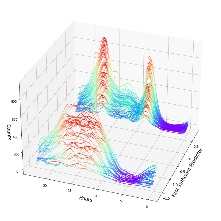
(a) First Direction

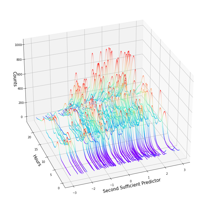
(b) Working Days

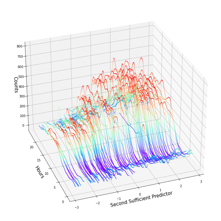
(c) Non-Working Days

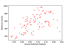
(d) Working Days

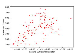
(e) Non-Working Days

Figure 1: (a) Plot of rental bike counts versus the first sufficient predictor in randomly selected 100 days; (b)(c) Plots of rental bike counts versus the second sufficient predictor for working days and non-working days based on the GWIRE estimates; (d)(e) Plots of the maximum counts of bike rental distributions versus the second sufficient predictor on working days and non-working days.

6 Discussion

This paper constructs a general framework for Fréchet SDR with a metric-space valued response and high-dimensional predictors. In particular, we propose a novel optimization problem to avoid the inverse of a large covariance matrix and leverage graphical information among predictors. We also establish the subspace estimation and variable selection consistency for the proposed estimator. Furthermore, most SDR approaches including SIR and CUME can be used in our procedure. We conclude with two open directions associated with this work. (a) It is of independent interest to construct confidence intervals (ellipsoids) and tests for coefficients of SDR. (b) Another direction is to extend our procedure to situations where predictors are tensors, functions, or random objects in metric space.

References

• Bhattacharjee and Müller (2021) Satarupa Bhattacharjee and Hans-Georg Müller. Single index Fréchet regression. arXiv:2108.05437, 2021.
• Boyd et al. (2011) Stephen Boyd, Neal Parikh, Eric Chu, Borja Peleato, and Jonathan Eckstein. Distributed optimization and statistical learning via the alternating direction method of multipliers. Foundations and Trends® in Machine learning, 3(1):1–122, 2011.
• Chen et al. (2010) Xin Chen, Changliang Zou, and R. Dennis Cook. Coordinate-independent sparse sufficient dimension reduction and variable selection. Ann. Statist., 38(6):3696–3723, 2010. ISSN 0090-5364. doi: 10.1214/10-AOS826. URL https://doi.org/10.1214/10-AOS826.
• Cook (1998) R Dennis Cook. Regression Graphics: Ideas for Studying Regressions through Graphics. John Wiley & Sons, 1998.
• Cook and Weisberg (1991) R Dennis Cook and Sanford Weisberg. Discussion of ‘sliced inverse regression for dimension reduction’. J. Amer. Statist. Assoc., 86(414):328–332, 1991.
• Fanaee-T and Gama (2014) Hadi Fanaee-T and Joao Gama. Event labeling combining ensemble detectors and background knowledge. Progress in Artificial Intelligence, 2(2):113–127, 2014.
• Friedman et al. (2008) Jerome Friedman, Trevor Hastie, and Robert Tibshirani. Sparse inverse covariance estimation with the graphical lasso. Biostatistics, 9(3):432–441, 2008.
• Lauritzen (1996) Steffen L Lauritzen. Graphical models, volume 17. Clarendon Press, 1996.
• Li (2018) Bing Li. Sufficient dimension reduction: Methods and applications with R. Chapman and Hall/CRC, 2018.
• Li and Li (2008) Caiyan Li and Hongzhe Li. Network-constrained regularization and variable selection for analysis of genomic data. Bioinformatics, 24(9):1175–1182, 2008.
• Li (1991) Ker-Chau Li. Sliced inverse regression for dimension reduction. J. Amer. Statist. Assoc., 86(414):316–342, 1991. ISSN 0162-1459. URL http://links.jstor.org/sici?sici=0162-1459(199106)86:414<316:SIRFDR>2.0.CO;2-V&origin=MSN. With discussion and a rejoinder by the author.
• Li (1992) Ker-Chau Li. On principal Hessian directions for data visualization and dimension reduction: another application of Stein’s lemma. J. Amer. Statist. Assoc., 87(420):1025–1039, 1992. ISSN 0162-1459. URL http://links.jstor.org/sici?sici=0162-1459(199212)87:420<1025:OPHDFD>2.0.CO;2-J&origin=MSN.
• Li and Yin (2008) Lexin Li and Xiangrong Yin. Sliced inverse regression with regularizations. Biometrics, 64(1):124–131, 323, 2008. ISSN 0006-341X. doi: 10.1111/j.1541-0420.2007.00836.x. URL https://doi.org/10.1111/j.1541-0420.2007.00836.x.
• Li and Zhang (2017) Lexin Li and Xin Zhang. Parsimonious tensor response regression. J. Amer. Statist. Assoc., 112(519):1131–1146, 2017. ISSN 0162-1459. doi: 10.1080/01621459.2016.1193022. URL https://doi.org/10.1080/01621459.2016.1193022.
• Lin et al. (2019) Qian Lin, Zhigen Zhao, and Jun S. Liu. Sparse sliced inverse regression via Lasso. J. Amer. Statist. Assoc., 114(528):1726–1739, 2019. ISSN 0162-1459. doi: 10.1080/01621459.2018.1520115. URL https://doi.org/10.1080/01621459.2018.1520115.
• Liu et al. (2019) Jianyu Liu, Guan Yu, and Yufeng Liu. Graph-based sparse linear discriminant analysis for high-dimensional classification. J. Multivariate Anal., 171:250–269, 2019. ISSN 0047-259X. doi: 10.1016/j.jmva.2018.12.007. URL https://doi.org/10.1016/j.jmva.2018.12.007.
• Luo and Li (2016) Wei Luo and Bing Li. Combining eigenvalues and variation of eigenvectors for order determination. Biometrika, 103(4):875–887, 2016.
• Obozinski et al. (2011) Guillaume Obozinski, Laurent Jacob, and Jean-Philippe Vert. Group lasso with overlaps: the latent group lasso approach. arXiv:1110.0413, 2011.
• Petersen and Müller (2016) Alexander Petersen and Hans-Georg Müller. Functional data analysis for density functions by transformation to a Hilbert space. Ann. Statist., 44(1):183–218, 2016. ISSN 0090-5364. doi: 10.1214/15-AOS1363. URL https://doi.org/10.1214/15-AOS1363.
• Petersen and Müller (2019) Alexander Petersen and Hans-Georg Müller. Fréchet regression for random objects with Euclidean predictors. Ann. Statist., 47(2):691–719, 2019. ISSN 0090-5364. doi: 10.1214/17-AOS1624. URL https://doi.org/10.1214/17-AOS1624.
• Peyré (2009) Gabriel Peyré. Manifold models for signals and images. Computer vision and image understanding, 113(2):249–260, 2009.
• Qian et al. (2019) Wei Qian, Shanshan Ding, and R. Dennis Cook. Sparse minimum discrepancy approach to sufficient dimension reduction with simultaneous variable selection in ultrahigh dimension. J. Amer. Statist. Assoc., 114(527):1277–1290, 2019. ISSN 0162-1459. doi: 10.1080/01621459.2018.1497498. URL https://doi.org/10.1080/01621459.2018.1497498.
• Small (2012) Christopher G Small. The statistical theory of shape. Springer Science & Business Media, 2012.
• Tan et al. (2020) Kai Tan, Lei Shi, and Zhou Yu. Sparse SIR: optimal rates and adaptive estimation. Ann. Statist., 48(1):64–85, 2020. ISSN 0090-5364. doi: 10.1214/18-AOS1791. URL https://doi.org/10.1214/18-AOS1791.
• Tan et al. (2018) Kean Ming Tan, Zhaoran Wang, Tong Zhang, Han Liu, and R Dennis Cook. A convex formulation for high-dimensional sparse sliced inverse regression. Biometrika, 105(4):769–782, 2018.
• Tang et al. (2020) Cheng Yong Tang, Ethan X. Fang, and Yuexiao Dong. High-dimensional interactions detection with sparse principal Hessian matrix. J. Mach. Learn. Res., 21:Paper No. 19, 25, 2020. ISSN 1532-4435.
• Tucker et al. (2021) Danielle C. Tucker, Yichao Wu, and Hans-Georg Müller. Variable selection for global Fréchet regression. J. Amer. Statist. Assoc., 0(0):1–15, 2021. doi: 10.1080/01621459.2021.1969240. URL https://doi.org/10.1080/01621459.2021.1969240.
• Weng (2022) Jiaying Weng. Fourier transform sparse inverse regression estimators for sufficient variable selection. Comput. Statist. Data Anal., 168:Paper No. 107380, 19, 2022. ISSN 0167-9473. doi: 10.1016/j.csda.2021.107380. URL https://doi.org/10.1016/j.csda.2021.107380.
• Weng and Yin (2018) Jiaying Weng and Xiangrong Yin. Fourier transform approach for inverse dimension reduction method. J. Nonparametr. Stat., 30(4):1049–1071, 2018. ISSN 1048-5252. doi: 10.1080/10485252.2018.1515432. URL https://doi.org/10.1080/10485252.2018.1515432.
• Weng and Yin (2022) Jiaying Weng and Xiangrong Yin. A minimum discrepancy approach with Fourier transform in sufficient dimension reduction. Statist. Sinica, 32(Special onlline issue):2381–2403, 2022. ISSN 1017-0405.
• Yin and Hilafu (2015) Xiangrong Yin and Haileab Hilafu. Sequential sufficient dimension reduction for large $p$, small $n$ problems. J. R. Stat. Soc. Ser. B. Stat. Methodol., 77(4):879–892, 2015. ISSN 1369-7412. doi: 10.1111/rssb.12093. URL https://doi.org/10.1111/rssb.12093.
• Ying and Yu (2022) Chao Ying and Zhou Yu. Fréchet sufficient dimension reduction for random objects. Biometrika, 02 2022. ISSN 1464-3510. doi: 10.1093/biomet/asac012. URL https://doi.org/10.1093/biomet/asac012.
• Yu and Liu (2016) Guan Yu and Yufeng Liu. Sparse regression incorporating graphical structure among predictors. J. Amer. Statist. Assoc., 111(514):707–720, 2016. ISSN 0162-1459. doi: 10.1080/01621459.2015.1034319. URL https://doi.org/10.1080/01621459.2015.1034319.
• Yu et al. (2016a) Zhou Yu, Yuexiao Dong, and Jun Shao. On marginal sliced inverse regression for ultrahigh dimensional model-free feature selection. Ann. Statist., 44(6):2594–2623, 2016a. ISSN 0090-5364. doi: 10.1214/15-AOS1424. URL https://doi.org/10.1214/15-AOS1424.
• Yu et al. (2016b) Zhou Yu, Yuexiao Dong, and Li-Xing Zhu. Trace pursuit: a general framework for model-free variable selection. J. Amer. Statist. Assoc., 111(514):813–821, 2016b. ISSN 0162-1459. doi: 10.1080/01621459.2015.1050494. URL https://doi.org/10.1080/01621459.2015.1050494.
• Zeng et al. (2022) Jing Zeng, Qing Mai, and Xin Zhang. Subspace estimation with automatic dimension and variable selection in sufficient dimension reduction. J. Amer. Statist. Assoc., 0(0):1–13, 2022. doi: 10.1080/01621459.2022.2118601. URL https://doi.org/10.1080/01621459.2022.2118601.
• Zhang et al. (2021) Qi Zhang, Lingzhou Xue, and Bing Li. Dimension reduction and data visualization for Fréchet regression. arXiv:2110.00467, 2021.
• Zhu et al. (2010) Li-Ping Zhu, Li-Xing Zhu, and Zheng-Hui Feng. Dimension reduction in regressions through cumulative slicing estimation. J. Amer. Statist. Assoc., 105(492):1455–1466, 2010. ISSN 0162-1459. doi: 10.1198/jasa.2010.tm09666. URL https://doi.org/10.1198/jasa.2010.tm09666.
• Zhu et al. (2013) Yunzhang Zhu, Xiaotong Shen, and Wei Pan. Simultaneous grouping pursuit and feature selection over an undirected graph. J. Amer. Statist. Assoc., 108(502):713–725, 2013. ISSN 0162-1459. doi: 10.1080/01621459.2013.770704. URL https://doi.org/10.1080/01621459.2013.770704.