Accelerated Bayesian Inference for Molecular Simulations using Local Gaussian Process Surrogate Models

Abstract

While Bayesian inference is the gold standard for uncertainty quantification and propagation, its use within physical chemistry encounters formidable computational barriers. These bottlenecks are magnified for modeling data with many independent variables, such as X-ray/neutron scattering patterns and electromagnetic spectra. To address this challenge, we apply a Bayesian framework accelerated via local Gaussian process (LGP) surrogate models. We show that the time-complexity of LGPs scales linearly in the number of independent variables, in stark contrast to the computationally expensive cubic scaling of conventional Gaussian processes. To illustrate the method, we trained a LGP surrogate model on the experimental radial distribution function of liquid neon, and observed a remarkable 288,000-fold speed-up compared to molecular dynamics with insignificant loss in predictive accuracy. We conclude that LGPs are robust and efficient surrogate models, poised to expand the application of Bayesian inference in molecular simulations to a broad spectrum of ever-advancing experimental data.

1 Introduction

Molecular simulations are becoming increasingly able to estimate complex experimental observables, including scattering patterns from neutron and X-ray sources and spectra from near-infrared [1], terrahertz [2], sum frequency generation [3, 4], and nuclear magnetic resonance [5]. Recent interest in these experiments to study hydrogen bonding networks of water at interfaces [6, 7], electrolyte solutions [8], and biological systems [9] has motivated the continued advancement of simulations to calculate these properties from first-principles [10, 11, 12]. However, the significant computational expense of molecular simulation greatly limits our understanding of how experimental, model, and parametric uncertainty impact these predictions. Without this understanding, it is difficult to know whether a model is an appropriate representation of nature or if it is simply over-fitting to a given training set. Therefore, what is needed is a computationally efficient and rigorous uncertainty quantification/propagation (UQ/P) method to link molecular models to complex experimental data.

Bayesian methods are the gold standard for these aims [13], with examples spanning from neutrino and dark matter detection [14], materials discovery and characterization [15, 16, 17], quantum dynamics [18, 19], to molecular simulation [20, 21, 22, 23, 24, 25, 26, 27, 28, 29, 30]. The Bayesian probabilistic framework is a rigorous, systematic approach to quantify probability distribution functions on model parameters and credibility intervals on model predictions, enabling robust and reliable parameter optimization and model selection [31, 32]. Interest in Bayesian methods for molecular simulation has surged [33, 34, 35, 36, 37] due to its flexible and reliable estimation of uncertainty, ability to identify weaknesses or missing physics in molecular models, and systematically quantify the credibility of simulation predictions. Additionally, standard inverse methods including relative entropy minimization, iterative Boltzmann inversion, and force matching have been shown to be approximations to a more general Bayesian field theory [38].

The biggest problem plaguing Bayesian inference is its massive computational cost. The two major computational pinch points are (1) sampling in high-dimensional spaces, commonly known as the "curse of dimensionality", and (2) the large number of model evaluations required to get accurate uncertainty estimates. For molecular simulation, these bottlenecks are magnified because molecular simulations are expensive. Therefore, rigorous and accurate uncertainty estimation is challenging, or even impossible, without accelerating the simulation prediction time. One way to achieve this speed-up is by approximating simulation outputs with an inexpensive machine learning model. These so-called surrogate models have been developed from neural networks [28, 39], polynomial chaos expansions [40, 41], configuration-sampling-based methods [42] and Gaussian processes [43, 44, 45].

Gaussian processes (GPs) are a compelling choice as surrogate models thanks to several distinct advantages. GPs are non-parametric, kernel-based function approximators that can interpolate function values in high-dimensional input spaces. GPs with an appropriately selected kernel also have analytical derivatives and Fourier transforms, making them well-suited for physical quantities such as potential energy surfaces [46] and structural correlations [47]. Additionally, kernels can encode physics-informed prior knowledge, alleviating the "black box" nature inherent to many machine learning algorithms. In fact, a comparison of various nonlinear regressors for molecular representations of ground-state electronic properties in organic molecules demonstrated that kernel regressors drastically outperformed other techniques, including convolutional graph neural networks [48].

Despite the numerous advantages of GPs, their adoption for Bayesian inference in physical chemistry remains limited. Bayesian inference on the self-diffusion coefficient and radial distribution function (RDF) of gaseous and liquid argon has been demonstrated using a highly-parallelizable transitional Markov chain Monte Carlo method with an adaptive GP surrogate model [49, 50]. These studies clearly show that using advanced sampling methods can drastically reduce computational cost. However, prior work in physical chemistry applications has not emphasized improving the computational efficiency of the GP surrogate model directly. This is significant since GPs have a cubic time-complexity in the number of independent variables (e.g. frequencies measured along a spectrum or radii measured along a RDF), which becomes more expensive as we include more data types into the Bayesian inference and as experimental measurements obtain higher ranges and resolution.

There is an emerging class of accelerated GP methods that are well-equipped to handle large sets of experimental data. Local Gaussian processes (LGPs) are constructed by separating a GP into a set of GPs trained at distinct locations in the input space [44, 51, 52, 53]. Computation on the LGP subset is trivially parallelizable and easily implemented in high-performance computing (HPC) architectures [54, 55]. State-of-the-art LGP models have been used to design Gaussian approximation potentials (GAPs) [56], a type of machine learning potential used to study atomic [57, 58, 59] and electron structures [60, 56], as well as nuclear magnetic resonance chemical shifts [61]. However, to our knowledge LGPs have not been applied as molecular simulation surrogate models for complex experimental observables.

In this study, we detail a simple and effective LGP surrogate model approach for complex experimental measurements common in physical chemistry. We show that the LGP approximation reduces the GP surrogate model evaluation time-complexity with respect to the number of QOIs from cubic to linear. The computational speed-up results from reducing the dimensionality of matrix operations and therefore enables Bayesian UQ/P on large scale experimental datasets. For example, consider that a typical Fourier transformed infrared spectroscopy (FT-IR) measurement may contain data between 4000-400 cm^-1 at a resolution of 2 cm^-1, giving a total number of QOIs around $\eta=1800$. According to the time-complexity scaling in $\eta$, we estimate that a LGP would accelerate this computation compared to a standard GP by approximately 3,240,000x.

As a direct application of the method, we trained a LGP surrogate model on a neutron scattering derived RDF for liquid neon (Ne). The LGP surrogate is found to reproduce the $\eta=73$ independent variable output space approximately 288,000x faster than molecular dynamics (MD) and 3500x faster than a conventional GP with accuracy comparable to the uncertainty in the reported experimental data (RMSE = 0.02). Accelerated Bayesian inference of the RDF under a ($\lambda$-6) Mie model is then used to draw conclusions on model behavior, uncertainty, and adequacy. Surprisingly, we find evidence that the ($\lambda$-6) Mie model is too inflexible to match fine structural details of liquid neon, highlighting opportunities for improving force field optimization and design.

2 Computational Methods

Bayes’ law, derived from the definition of conditional probability, is a formal statement of revising one’s prior beliefs based on new observations. Bayes’ theorem for a given model, set of model input parameters, $\boldsymbol{\theta}$, and set of experimental QOIs, $\mathbf{y}$, is expressed as,

$$p(\boldsymbol{\theta}|\mathbf{y})\propto p(\mathbf{y}|\boldsymbol{\theta})p(\boldsymbol{\theta})$$ (1)

where $p(\boldsymbol{\theta})$ is the ’prior’ probability distribution over the model parameters, $p(\mathbf{y}|\boldsymbol{\theta})$ is the ’likelihood’ of observing $\mathbf{y}$ given parameters $\boldsymbol{\theta}$, and $p(\boldsymbol{\theta}|\mathbf{y})$ is the ’posterior’ probability that the underlying parameter $\boldsymbol{\theta}$ models or explains the observation $\mathbf{y}$. Equality holds in eq (1) if the right-hand-side is normalized by the ’marginal likelihood’, $p(\mathbf{y})$, but including this term explicitly is unnecessary since the posterior probability distribution can be normalized post hoc. In molecular simulations, $\boldsymbol{\theta}$ is the set of parameters that we want to optimize in the selected model, usually the force field parameters in the Hamiltonian, to the experimental QOI that we expect the simulation to reproduce. The observations, $\mathbf{y}$, can be any QOI or combination of QOIs (e.g. RDFs, spectra, densities, diffusivities, etc). This construction, known as the standard Bayesian scheme, is generalizable to any physical model and its corresponding parameters including density functional theory, ab initio molecular dynamics, and path integral molecular dynamics.

Calculating the posterior distribution then just requires prescription of prior distributions on the model input parameters and evaluation of the likelihood function. In this work, we employ Gaussian distributions for both the prior and likelihood functions, which is a standard choice according to the central limit theorem. The Gaussian likelihood has the form,

$$p(\mathbf{y}|\boldsymbol{\theta})=\bigg{(}\frac{1}{\sqrt{2\pi}\sigma_{n}}\bigg{)}^{\eta}\exp\bigg{[}-\frac{1}{2\sigma_{n}^{2}}\sum_{i}\ [\mathbf{y}_{\boldsymbol{\theta}}-\mathbf{y}]^{2}\bigg{]}$$ (2)

where $\eta$ is the number of observables in $\mathbf{y}$, $\sigma_{n}$ is a nuisance parameter describing the unknown variance of the Gaussian likelihood, and $\mathbf{y}_{\boldsymbol{\theta}}$ is the model predicted observables at model input $\boldsymbol{\theta}$. Note that in some cases a different likelihood function may be more appropriate based on physics-informed prior knowledge of the distribution of the observable of interest (e.g. the multinomial likelihood in relative entropy minimization between canonical ensembles [62]).

The computationally expensive part of calculating eq 2 is determining $\mathbf{y}_{\boldsymbol{\theta}}$ at a sufficient number of points in the parameter space. Generally, this can be achieved by calculating $\mathbf{y}_{\boldsymbol{\theta}}$ at dense, equally spaced points in the parameter space of interest (grid method), sampling the parameter space with Markov chain Monte Carlo (MCMC) to estimate the posterior with a histogram (approximate sampling method), or assuming that the posterior distribution has a specific functional form (i.e. Laplace approximation). Regardless of the selected method, each of these posterior distribution characterization techniques require a prohibitive number of molecular simulations (often on the order of $10^{5}-10^{6}$) to adequately sample the parameter space, which is completely infeasible for even modest sized molecular systems.

2.1 Gaussian Process Surrogate Models

GPs accelerate the Bayesian likelihood evaluation by approximating $\mathbf{y}_{\boldsymbol{\theta}}$ with an inexpensive matrix calculation. Therefore, GP surrogate models offer a cost-effective substitute for computationally expensive molecular simulations. By leveraging matrix-based approximations, this ML-accelerated approach enables the efficient calculation of extensive sets of thermodynamic data at a scale that is infeasible for molecular simulations.

A Gaussian process is a stochastic process such that every finite set of random variables (position, time, etc) has a multivariate normal distribution [43]. The joint distribution over all random variables in the system therefore defines a probability distribution over functions. The expectation of this distribution maps a set of model parameters, $\boldsymbol{\theta}^{*}$, and independent variables, $\mathbf{r}$, to the most probable QOI function, $S(\mathbf{r}|\boldsymbol{\theta}^{*})$, such that,

$$\mathbb{E}[GP]:\boldsymbol{\theta}^{*}\times\mathbf{r}\mapsto S(\mathbf{r}|\boldsymbol{\theta}^{*})$$ (3)

where the expectation operator is written in terms of a kernel matrix, $\mathbf{K}$, training set parameter matrix, $\mathbf{\hat{X}}$, and training set output matrix, $\mathbf{\hat{Y}}$, according to the equation,

$$\mathbb{E}[\textit{GP}(\boldsymbol{\theta}^{*},\mathbf{r})]=\mathbf{K}_{(\boldsymbol{\theta}^{*},\mathbf{r}),\mathbf{\hat{X}}}[\mathbf{K}_{\mathbf{\hat{X}},\mathbf{\hat{X}}}+\sigma_{noise}^{2}\mathbf{I}]^{-1}\mathbf{\hat{Y}}$$ (4)

where $\sigma_{noise}^{2}$ is the variance due to noise and $\mathbf{I}$ is the identity matrix. Note that in general the independent variables, $\mathbf{r}$, can be multidimensional. As an example, consider the case where we want a GP to map a set of force field parameters to the angular RDF of a liquid. We now have a 2-dimensional space of independent variables since the angular RDF gives the atomic density along the radial and angular dimensions. Another example is if one wanted to build a GP for an RDF and FT-IR spectra simultaneously. In the following mathematical development, we assume that the QOI is 1-dimensional for the sake of notational convenience and note that extending the argument to higher-dimensional observables is trivial.

The kernel matrix, $\mathbf{K}$, quantifies the relatedness between input parameters and can be selected based on prior knowledge of the physical system. A standard kernel for physics-based applications is the squared-exponential (or radial basis function) since the resulting GP is infinitely differentiable, smooth, continuous, and has an analytical Fourier transform [63]. The squared-exponential kernel function between input points $(\boldsymbol{\theta}_{m},r_{m})$ and $(\boldsymbol{\theta}_{n},r_{n})$ is given by,

$$K_{mn}=\alpha^{2}\exp\bigg{(}-\frac{(r_{m}-r_{n})^{2}}{2\ell_{r}^{2}}-\sum_{o=1}^{\text{dim}(\boldsymbol{\theta})}\frac{(\theta_{o,m}-\theta_{o,n})^{2}}{2\ell_{\theta_{o}}^{2}}\bigg{)}$$ (5)

where $o$ indexes over dim($\boldsymbol{\theta}$) and the hyperparameters $\alpha^{2}$ and $\ell_{A}$ are the kernel variance and correlation length scale of parameter $A$, respectively. Hyperparameter optimization can be performed by log marginal likelihood maximization, $k$-fold cross validation [43] or marginalization with an integrated acquisition function [64], but can be computationally expensive and is usually avoided if accurate estimates of the hyperparameters can be made from prior knowledge of the chemical system.

To train a standard GP surrogate model, we need to generate $N$ training samples in the input parameter space and run a molecular simulation for each training set sample to calculate $N$ predictions over the number of target QOIs, $\eta$. The training set, $\mathbf{\hat{X}}$, is then a ($N\eta$ $\times$ dim($\boldsymbol{\theta}$) + 1) matrix of the following form,

$$\mathbf{\hat{X}}=\begin{bmatrix}\theta_{1,1}&\theta_{2,1}&\ldots&r_{1}\\ \theta_{1,1}&\theta_{2,1}&\ldots&r_{2}\\ \vdots&\vdots&\vdots&\vdots\\ \theta_{1,1}&\theta_{2,1}&\ldots&r_{\eta}\\ \theta_{1,2}&\theta_{2,2}&\ldots&r_{1}\\ \vdots&\vdots&\vdots&\vdots\\ \theta_{1,N}&\theta_{2,N}&\ldots&r_{\eta}\\ \end{bmatrix}$$ (6)

where the $\theta_{i,j}$ are the $i^{th}$ model parameter for sample index $j$ and $r_{k}$ are the independent variables of the target QOI. Note that the training sample index, $j=1,...,N$, is updated in the model parameters only after $\eta$ rows spanning the domain of the observable, giving $N\eta$ total rows. Therefore, the training set matrix represents all possible combinations of the training parameters in the $\boldsymbol{\theta}$ parameter input space.

The training set observations, $\mathbf{\hat{Y}}$, is then a ($N\eta$ $\times$ 1) column vector of the observable outputs from the training set,

$$\mathbf{\hat{Y}}=[S(\boldsymbol{\theta}_{1},r_{1}),...,S(\boldsymbol{\theta}_{1},r_{\eta}),S(\boldsymbol{\theta}_{2},r_{1}),...,S(\boldsymbol{\theta}_{N},r_{\eta})]^{T}$$ (7)

where $S(\boldsymbol{\theta}_{j},r_{k})$ is the training set observation of model parameters $\theta_{j}$ at independent variable $r_{k}$. The expectation of the GP for a new set of parameters, $S(\mathbf{r}|\boldsymbol{\theta}^{*})$, is then a ($\eta$ x 1) column vector calculated with eq (4) to give the most probable QOI output,

$$S^{*}(\mathbf{r}|\boldsymbol{\theta}^{*})=[S^{*}(r_{1}|\boldsymbol{\theta}^{*}),...,S^{*}(r_{\eta}|\boldsymbol{\theta}^{*})]^{T}.$$ (8)

The GP expectation calculation is burdened by the inversion of the training-training kernel matrix with $\mathcal{O}(N^{3}\eta^{3})$ time complexity and the ($\eta$ $\times$ $N\eta$) $\times$ ($N\eta$ $\times$ $N\eta$) $\times$ ($N\eta$ $\times$ 1) matrix product with $\mathcal{O}(N^{2}\eta^{3})$ time complexity. Note that these estimates are for naive matrix multiplication. Regardless, the cubic scaling in $\eta$ dominates the time-complexity for observables with many QOIs. For example, to build a GP surrogate model for the density of a noble gas ($\eta=1$) with Lennard-Jones interactions (dim($\boldsymbol{\theta}$) = 2) would give a training set matrix of ($2N\times 3)$. Similarly, a surrogate model for an infrared spectrum of water from 600-4000 cm^-1 at a resolution of $4$ cm^-1 ($\eta=850$) estimated with a 3 point water model of Lennard-Jones type interactions (dim($\boldsymbol{\theta}$) = 6) would generate a training set matrix of size (850$N$ $\times$ 7). Clearly, the complexity of the output QOI causes a significant increase in the computational cost of matrix operations.

2.2 The Local Gaussian Process Surrogate Model

The time-complexity of the training-kernel matrix inversion and the matrix product can be substantially reduced by fragmenting the full Gaussian process of eq (4) into $\eta$ Gaussian processes along the independent variables of the QOI. Under this construction, an individual $GP_{k}$ is trained to map a set of model parameters to an individual QOI,

$$\mathbb{E}[GP_{k}]:\boldsymbol{\theta}\mapsto S(r_{k})$$ (9)

where $\mathbf{r}$ is no longer an input parameter. The training set matrix, $\mathbf{\hat{X^{\prime}}}$, is now a ($N$ $\times$ dim($\boldsymbol{\theta}$)) matrix,

$$\mathbf{\hat{X^{\prime}}}=\begin{bmatrix}\theta_{1,1}&\theta_{2,1}&\ldots\\ \theta_{1,2}&\theta_{2,2}&\ldots\\ \vdots&\vdots&\vdots\\ \theta_{1,N}&\theta_{2,N}&\ldots\\ \end{bmatrix}$$ (10)

while the training set observations, $\mathbf{\hat{Y^{\prime}}}_{k}$, is a ($N$ $\times$ 1) column vector of the QOIs from the training set at $r_{k}$,

$$\mathbf{\hat{Y}^{\prime}}_{k}=[S(\boldsymbol{\theta}_{1},r_{k}),...,S(\boldsymbol{\theta}_{N},r_{k})]^{T}$$ (11)

where the $k$ indexes over independent variables. The LGP surrogate model prediction for the observable at $r_{k}$, $S_{loc}^{*}(r_{k})$, at a new set of parameters, $\boldsymbol{\theta}^{*}$, is just the expectation of the $k^{th}$ Gaussian process given the training set data,

$$S_{loc}^{*}(r_{k})=\mathbb{E}[\textit{GP}_{k}(\boldsymbol{\theta}^{*})]=\mathbf{K}_{\boldsymbol{\theta}^{*},\mathbf{\hat{X^{\prime}}}}[\mathbf{K}_{\mathbf{\hat{X^{\prime}}},\mathbf{\hat{X^{\prime}}}}+\sigma_{noise}^{2}\mathbf{I}]^{-1}\mathbf{\hat{Y^{\prime}}}_{k}$$ (12)

We can then just combine the local results from the subset of $\eta$ GPs to obtain a prediction for the QOIs,

$$S_{loc}^{*}(\mathbf{r})=[S_{loc}^{*}(r_{1}),...,S_{loc}^{*}(r_{\eta})]^{T}.$$ (13)

By reducing the dimensionality of the relevant matrices, the time complexity of the matrix calculations are drastically reduced compared to a standard GP. The single step inversion of the training-training kernel matrix is now of $\mathcal{O}(N^{3})$ time complexity while the $\eta$ step (1 $\times$ $N$) $\times$ ($N$ $\times$ $N$) $\times$ ($N$ $\times$ 1) matrix products are reduced to $\mathcal{O}(N^{2}\eta)$ time complexity. If the number of training samples, $N$, the number of independent variables, $\eta$, and the number of model evaluations, $G$, are equal between the full and LGP algorithms, then a LGP approximation reduces the evaluation time complexity in a standard GP from cubic-scaling, $\eta^{3}$, to embarrassingly parallel linear-scaling, $\eta$.

In summary, a local Gaussian process is an approximation in which all of the QOIs are modeled as independent random variables, each described by their own Gaussian process. This amounts to assuming that the random variables are independent and identically distributed (i.i.d.), which may or may not be true for a given experimental observation. For time-independent data including scattering measurements and spectroscopy, this approximation is appropriate since each observation is an independent measurement at each independent variable. In contrast, this approximation would not hold for time-dependent data in which a measurement at time $t$ depends on previous measurements $t_{i}<t$.

We show that complex experimental observables can be reconstructed by this set of LGPs through a series of relatively straightforward matrix operations with linear time-complexity with respect to the number of independent variables. We also note that the LGP has all of the primary advantages of Bayesian methods, including built-in UQ and analytical derivatives and Fourier transforms. In the following section, we show the computational enhancement and accuracy of the LGP approach by modeling the RDF of neon at 42$K$. We then use the surrogate model within a Bayesian framework to exemplify the power of UQ/P for molecular simulations.

3 A Local Gaussian Process Surrogate for the RDF of Liquid Ne

To explore the computational advantages of LGP surrogate models for Bayesian inference, we studied the experimental RDF of liquid Ne [65] under a ($\lambda$-6) Mie fluid model. The ($\lambda$-6) Mie force field is flexible Lennard-Jones type potential with variable repulsive exponent,

$$v^{Mie}_{2}(r)=\frac{\lambda}{\lambda-6}\bigg{(}\frac{\lambda}{6}\bigg{)}^{\frac{6}{\lambda-6}}\epsilon\bigg{[}\bigg{(}\frac{\sigma}{r}\bigg{)}^{\lambda}-\bigg{(}\frac{\sigma}{r}\bigg{)}^{6}\bigg{]}$$ (14)

where $\lambda$ is the short-range repulsion exponent, $\sigma$ is the collision diameter ($\mathrm{\text{\r{A}}}$), and $\epsilon$ is the dispersion energy (kcal/mol) [66].

MD simulations were performed from a sobol sampled set spanning a prior range based on existing force field models [67, 68, 69] ($\lambda=[5,20]$, $\sigma=[1.5,4.0]$, and $\epsilon=[0,0.5]$) to generate a RDF training set matrix of the form in eq 10. The number of training simulations performed was $N=480$, the number of $r$ points in the experimental RDF was $\eta=73$, and the number of surrogate model calls is $G=8\times 10^{5}$. The number of points $\eta$ in the radial distribution was calculated by dividing the reported $r_{max}-r_{min}\approx 15.3$ by the effective $r$-space resolution given by, $\Delta r=\pi/Q_{max}$, where $\Delta r=0.21$ $\mathrm{\text{\r{A}}}$ for reported $Q_{max}=15$ $$\mathrm{\text{\r{A}}}$^{-1}$. The total number of training simulations was selected based on a sequential sampling approach in which 160 simulations were performed and progressively narrowed based on the RMSE between the simulation and experimental RDF. Three iterations (480 total) was found to provide an RMSE similar to the reported experimental uncertainty. Details on the MD simulations, training set, and Bayesian framework are provided in the Appendix.

3.1 Computational Efficiency and Accuracy

Now that we have constructed the training set matrix, we simply evaluate the expectation at each $r$ according to eq (12) and combine the results into a single array as in eq (13). The average computational time to evaluate the RDF and invert the training set matrix are shown below in Table 1. The LGP surrogate model is found to accelerate the model QOI prediction time compared to MD by a factor of 287,984. Furthermore, this 5 orders-of-magnitude speed-up is shown to outpace a standard GP by 3 orders-of-magnitude (3533x). The total time to compute the Bayesian posterior distribution with MCMC was thereby reduced from an estimated $\sim$4.9 years for MD or $\sim$22 days for a standard GP surrogate model, to less than 9 minutes on our local cluster. In fact, the LGP is so fast that we can calculate the Bayesian likelihood without introducing non-trivial sampling techniques such as active learning and/or translational Markov chain Monte Carlo.

Table 1: Average relative time and speed-up to QOI evaluation and training set matrix inversion for a standard and local Gaussian process for a RDF with $\eta=73$ points.

Model	Time to QOI (s)	Speed Up ($t/t_{sim}$)	Inv. Time (s)	Inv. Speed Up ($t_{GP}/t_{LGP}$)
Simulation	86.25	1	-	-
GP	1.06	81.19	87	1
LGP	0.0003	287,984	0.02	4183

We’ve established that the LGP is fast, but is it accurate? In other words, does the LGP provide QOI predictions that are within a reasonable level of accuracy to serve as a true surrogate model for the MD? To evaluate the accuracy of the local predictions, we ran a 160 sample test set around the posterior distribution and computed the root mean squared error (RMSE) between simulated and LGP predicted radial distributions. The results are summarized in Figure 1.

The total RMSE over the test set gives a value of 0.02, which is excellent considering that this is less than the uncertainty reported in the experimental measurement ($\sim$0.03). A plot of the RMSE as a function $r$-coordinate reveals period and asymptotically decaying accuracy in $r$ corresponding approximately to the peak positions, which is expected because the magnitude of the RDF exhibits similar behavior. Overall, the LGP RMSE is considered excellent for a RDF, but could be improved by including additional training set samples.

Figure 1: (a)-(c) Test set samples over each parameter plotted against the RMSE between simulated and LGP data. (d) Average RMSE over the 160 test set samples as a function of $r$,

One notable limitation of the LGP surrogate model is that it may have numerical instabilities that reduce the accuracy of the GP posterior distribution [70, 71]. For this work, we argue that this limitation is minor since we do not use the GP posterior distribution directly; rather, we use only its expectation. However, if an application requires a high accuracy estimation of GP posterior distribution (e.g. active learning or forecasting), more advanced greedy approximation methods may be required [71, 70, 72, 73].

3.2 Learning from Surrogate Models with Bayesian Analysis

Our fast and accurate LGP surrogate model now allows us to explore the underlying probability distributions on the ($\lambda$-6) Mie parameter space. This example is provided to show how one can use Bayesian analysis to learn about correlations between model parameters, relationships between model parameters and the QOI, and model adequacy. This knowledge can provide deep insight into the nature of the model and provide quantifiable evidence for whether or not the model is appropriate for a target application.

Bayesian inference yields a probability distribution function over the model parameters called the joint posterior probability distribution. The maximum of the joint posterior, referred to as the maximum a posteriori (MAP), represents the set of parameters with the highest probability of explaining the given experimental data. In force field design, the MAP would be an appropriate choice for an optimal set of model parameters. However, the power of the Bayesian approach lies in the fact that, not only can we identify the optimal parameters, but we can also examine the probability distribution of the parameters around these optima. For instance, the width of the distribution provides evidence for how important a parameter in the model is for representing the target data. For a given parameter, a wide distribution indicates that the parameter has little influence on the model prediction. On the other hand, a narrow distribution indicates that the parameter is critical to the model prediction. Additionally, the joint posterior may exhibit multiple peaks, or modes. A multimodal joint posterior suggests that there are multiple sets of model parameters that reproduce the target data, which may be a symptom of model inadequacy. Finally, the symmetry of the distribution provides information on relationships and correlations between parameters, providing a framework to diagnose subtle relationships that may otherwise go unnoticed.

Usually, the joint posterior distribution is a high-dimensional quantity that cannot be visualized directly. However, we can visualize the joint posterior along one dimension by integrating out the contributions over all other parameters. The resulting distributions are called marginal distributions. Marginal distributions computed over the ($\lambda$-6) Mie potential parameters optimized to the RDF of liquid Ne are shown in Figure 2.

Figure 2: (a)-(c) 1D marginal distributions for the ($\lambda$-6) Mie fluid parameters. Blue lines are the prior distributions and red dotted lines represent the maximum a posterior (MAP). (d)-(f) 2D marginal histograms showing parameter correlations. Red marker indicates the 2D MAP.

For each parameter, the resulting marginal posterior distributions are unimodal and symmetric. This result is not surprising in the context of recent results that show iterative Boltzmann inversion, which is a maximum likelihood approach to the structural inverse problem, is convex for Lennard-Jones type fluids [74]. Observing the 2D marginal distributions in the second row of Figure 2, we can also see that each of the parameters are correlated to one other. For example, the negative correlation between $\sigma$ and $\epsilon$ suggests that increasing the size of the particle should be accompanied by a decrease in the effective particle attraction. Conceptually this makes sense, if the particles are larger, then they would need to have a weaker attractive force to give the same atomic structure. This result is consistent with Bayesian analysis on liquid Ar [49]. Quantitative analysis of model sensitivity can also be performed with probabilistic derivatives of the QOI with respect to model parameters (see Appendix).

One surprising characteristic of the posterior distribution is that it is extremely narrow. Recall that narrow distributions indicate that the parameters are important, or have tight control, over the model quality-of-fit to the experimental data. From our Bayesian analysis, we can therefore confidently conclude that detailed interatomic force information is contained within the experimental RDF. This observation is in stark contrast to over 60 years of prior literature which has unanimously asserted that only the excluded volume or collision diameter can be ascertained from experimental scattering data [75, 76, 77]. In fact, the Bayesian analysis shows that we can actually determine values for $\lambda$, $\sigma$, and $\epsilon$ within $\pm 1.5$, $\pm 0.03$\mathrm{\text{\r{A}}}$$, and $\pm 0.005$ kcal/mol with 95% certainty. This result leads to two important conclusions. First, scattering data effectively constrains the force field model parameter space. Second, scattering data must be accurate to design structure-optimized force fields.

The joint posterior can also be used for model parameter optimization. Specifically, the optimal parameters are given by the MAP, corresponding to the maximum of the joint posterior distribution. The MAP is presented in Table 2 along with two other existing force fields for liquid Ne.

Table 2: Summary of ($\lambda-6)$ Mie potential parameters optimized for Ne. Values for the repulsive exponent parameter are rounded to the nearest integer.

Force Field	QOI	$\lambda$	$\sigma$ ($\mathrm{\text{\r{A}}}$)	$\epsilon$ (kcal/mol)
Mick (2015)	VLE	11	2.794	0.064
SOPR (2022)	RDF	11	2.778	0.063
This Work	RDF	9.27	2.774	0.059

We can clearly see that the optimal repulsive exponent and dispersion energy prediction are lower than the Mick [68] and structure optimized potential refinement (SOPR) [69] models, while the optimal collision diameter is the same. Interestingly, the optimal $\epsilon$ parameter derived from SOPR falls just outside of the 95% credibility interval, despite being trained on the same experimental RDF. The difference between the Mie fluid and SOPR model is that the former is parametric while the latter is non-parametric, both of which have strengths and weaknesses. Specifically, parametric models are less complex but may not be flexible enough to describe subtle details of the experimental observation. On the other hand, non-parametric models can describe nuanced experiments but may over-fit to non-physical features of the data. It is then natural to wonder: Is the Mie model missing important physics? Or is the SOPR model over-fitting to imperfect data?

We can investigate these questions further by propagating parameter uncertainty through the Mie model to construct a distribution of RDF predictions - referred to as the posterior predictive. The posterior predictive quantifies of how accurately we know the QOI given experimental, model, and parametric uncertainty. If the model is adequate, the Bayesian credibility interval ($\mu\pm 2\sigma$) should contain approximately 95% of the experimental data. The posterior predictive and residuals ($g_{exp}(r)-\mu(r)$) for the liquid Ne RDF are shown in Figure 3.

Figure 3: (a) RDF mean and credibility interval propagated from the parameter uncertainty quantified with Bayesian inference. (b) Residual analysis comparing the experimental data with the Bayesian posterior distribution.

We notice that the residuals between the experiment and posterior predictive mean are evenly distributed but often lie outside of the 95% credibility interval. Therefore, the Mie model captures the general structural behavior of Ne but fails to describe nuanced features present in the RDF data. This result suggests that there are potentially missing physics that could be incorporated to better present the structural behavior of the fluid. We therefore suspect that the non-parametric SOPR model is capturing these more realistic interactions, which is supported by its excellent agreement with structure and thermodynamic properties. Of course, this remains an open hypothesis and should be scrutinized through empirical testing and uncertainty quantification of the SOPR method.

In summary, we have shown that a LGP surrogate model enables rapid and accurate uncertainty quantification and propagation with Bayesian inference. We then showed how the posterior distribution is an indispensable tool to learn subtle relationships between model parameters, identify how important each model parameter is to describe the outcome of experiments, and quantify our degree of belief that our model adequately describes our observations. The power of Bayesian inference is evident.

4 Conclusions

We have shown that local Gaussian process surrogate models trained on an experimental RDF of liquid neon improves the computational speed of QOI prediction nearly 300,000-fold with exceptional accuracy from only 480 training simulations. The 3 orders-of-magnitude evaluation time speed-up for a local versus standard Gaussian process was shown to accelerate Bayesian inference without the need for advanced sampling techniques such as on-the-fly learning. Furthermore, since the LGP linearly scales with the number of output QOIs, we expect significantly higher speed-up for more complex data, such as infrared spectra or high resolution scattering experiments, or for multiple data sources simultaneously (e.g. scattering, spectra, density, diffusivity, etc). We conclude that local Gaussian processes are an accurate and reliable surrogate modeling approach that can be extremely useful for Bayesian inference of molecular models over a broad array of complex experimental data.

5 Acknowledgements

This study is supported by the National Science Foundation Award No. CBET-1847340. We would like to thank Sean T. Smith and Philip J. Smith for their invaluable advice on the implementation of Gaussian processes.

6 Author Contributions

BL Shanks - conceptualization, formal analysis, code development, manuscript writing and preparation. HW Sullivan - conceptualization, formal analysis, code development, manuscript preparation. AR Shazed - molecular simulations. MP Hoepfner - conceptualization, funding acquisition, manuscript preparation.

7 Appendix

Appendix A Notes on Gaussian Process Hyperparameter Selection

The kernel of the Gaussian process depends on a set of hyperparameters that can influence the surrogate model prediction. A standard approach to selecting hyperparameters is to maximize the model evidence [43] or apply an expected improvement criterion based on an integrated acquisition function [64]. Here we have applied a brute force search based on minimizing the leave-one-out cross validation (LOOCV) error, which creates a limitation in the uncertainty quantification since we are not accounting for hyperparameter uncertainty. However, the self-consistency of our approach with other methods, including vapor-liquid equilibria optimized [68] and structure optimized potential refinement [69], suggests that this choice is appropriate for structural modeling in these systems. However, implementation of a fully Bayesian treatment of the Gaussian process hyperparameters may be necessary in more complex structural problems.

Appendix B Molecular Dynamics Simulation of Mie Fluids

Computer generated radial distribution functions were calculated using molecular dynamics (MD) simulations in the HOOMD-Blue package [78]. Simulations were initiated with a lattice configuration of 864 particles and compressed to a reduced density of $\rho=0.02477$ atom/$$\mathrm{\text{\r{A}}}$^{3}$ and temperature $T=42.2$ K. The HOOMD $NVT$ integrator was used for a 0.25 nanosecond equilibration step and a 0.25 nanosecond production step (dt = 0.5 femtosecond). Potentials were truncated at $3\sigma$ with an analytical tail correction, and radial distribution functions were calculated using the Freud package [79].

B.1 Constructing the Surrogate Model Training Set

To generate a useful training set, we need dense samples of model parameters in the region of the parameter space that can well-represent the target quantity-of-interest (QOI). However, it is not known a priori where this region is, particularly if there is no prior knowledge of what model parameters best represent the target observable. In this work, we use a sequential sampling approach in which we sample a wide range of parameters, determine the best-fit to the target observable, and then narrow the parameter range around this point for the next set of training samples. We repeated this procedure three times with 160 samples per iteration. A visualization of this procedure is shown below in Figure 4.

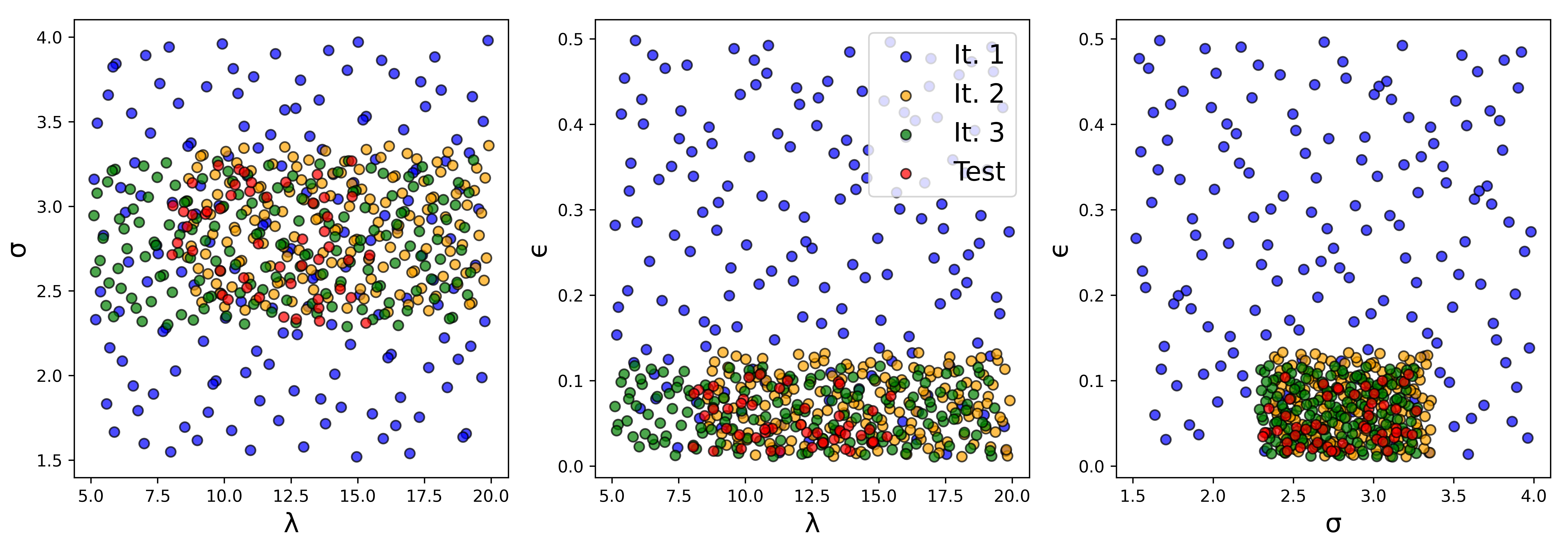
Figure 4: 2D training and sample parameter set used to train and evaluate the local Gaussian process surrogate model.

The updated range on the training set samples are centered on the parameters that provided the lowest RMSE compared to the experiment and the range was narrowed by a fixed interval based on inspection of the RMSE between the training set and the experimental data. One could also use an adaptive or on-the-fly learning approach in which the uncertainty in the local GP prediction is used to decide whether or not a new simulation is needed. This approach was used in prior work [49, 80] but was unnecessary in this study due to the efficiency and accuracy of the local GP.

Appendix C The Standard Bayesian Framework

Bayesian inference was implemented to calculate parameter probability distributions as a function of structure factor uncertainty. For simplicity of notation, let $\theta=\{\lambda,\sigma,\epsilon,s_{n}\}$ represent the model parameters and $\mathcal{Y}=S_{d}(Q)$ be the structure factor observations. The nuisance parameter, $s_{n}$, represents the width of the Gaussian likelihood and is considered an unknown model parameter since nothing is known about this parameter a priori. Calculating the posterior probability distribution with Bayesian inference then requires two components: (1) prescription of prior distributions on the model parameters, $p(\theta)$, and (2) evaluation of the likelihood, $p(\mathcal{Y}|\theta)$. The prior distribution over the $(\lambda-6)$ Mie parameters is assumed to be a multivariate normal distribution,

$$\theta\sim\mathcal{N}(\mu_{\theta},s^{2}_{\theta})$$ (15)

where $\mu_{\theta}$ and $s^{2}_{\theta}$ are the prior mean and variance of each $(\lambda-6)$ Mie parameter in $\theta$, respectively. A wide, multivariate normal distribution was selected because it is non-informative and conjugate to the Gaussian likelihood equation. The prior on the nuisance parameter is assumed to be log-normal,

$$\log s_{n}\sim\mathcal{N}(\mu_{s_{n}},s_{s_{n}}^{2})$$ (16)

where $\mu_{s_{n}}$ and $s_{s_{n}}$ are the prior mean and variance of the nuisance parameter. The log-normal prior imposes the constraint that the nuisance parameter is non-negative, which is obviously true because a negative variance in the observed data is undefined. For reference, the prior parameters used in this study are summarized in Table 3.

Table 3: Prior parameters on the ($\lambda$-6) Mie model parameters.

Parameter	Distribution	$\mu$	$s$
$\lambda$		12.0	9
$\sigma$	Normal	2.7	1.8
$\epsilon$		0.112	0.225
$s_{n}$	Log-Normal	1	1

The likelihood function is assumed to be Gaussian according to the central limit theorem,

$$p(\mathcal{Y}|\theta)\propto\frac{1}{s_{n}^{n_{samples}}}\exp\bigg{[}-\frac{1}{2s^{2}_{n}}\sum_{i}\ [{S}_{\theta_{i}}(Q_{j})-S_{d}(Q_{j})]^{2}\bigg{]}$$ (17)

where ${S}_{\theta}(Q_{i})$ is the molecular simulation predicted QOI and $j$ indexes over discrete independent variables of the QOI. Bayes’ theorem is then expressed as,

$$p(\theta|\mathcal{Y})\propto p(\mathcal{Y}|\theta)p(\theta)$$ (18)

where equivalence holds up to proportionality. This construction is acceptable since the resulting posterior distribution can be normalized post hoc to find a valid probability distribution.

To populate the Bayesian likelihood distribution, Markov Chain Monte Carlo (MCMC) samples are passed to the surrogate model, evaluated, and compared to the experimental RDF. 800,000 MCMC samples were calculated using the emcee package [81] using 160 walkers and a 1000 sample burn-in. The acceptance ratio obtained from this sampling procedure was $\sim$0.3 and the autocorrelation between steps was 15 moves.

Appendix D Sensitivity Analysis with Gaussian Process Derivatives

One of the most useful applications of Bayesian inference is parameter sensitivity analysis. As was shown in the main text, studying the correlations and shape of the joint posterior distribution can reveal insight into how parameters influence the prediction of a QOI. However, the joint posterior is not the only method to study parameter sensitivity. Specifically, analytical derivatives of the local GP surrogate model can directly quantify the differential rate of change of the QOI to a model parameter. As a demonstration, figure 5 plots local GP derivatives calculated for the ($\lambda$-6) Mie parameters.

We can now precisely study how each parameter changes the radial distribution function. For instance, the repulsive exponent derivative exhibits a small magnitude and has a minimum at the radial distribution function half maximum. This behavior suggests that increasing the repulsive exponent, which determines the "hardness" of the particles, steepens the slope of the first peak. This makes sense, just consider that in a hard-particle model there is a discontinuous jump at the hard-particle radius (infinite slope) that progressively softens with the introduction of an exponential repulsive decay function. In the case of the collision diameter, zeros of the derivative occur at structure factor peaks and troughs, while local extrema align with the half-maximum positions. Consequently, increasing the effective particle size shifts the radial distribution function to the right while maintaining relatively constant peak heights. Regarding the dispersion energy, its derivative displays zeros at the half-maximum positions of the structure factor and local extrema at peaks and troughs. This behavior indicates that an increase in the dispersion energy leads to an increased magnitude of the radial distribution function peaks and greater liquid structuring.

It is also possible to relate GP derivatives with thermodynamic variable derivatives. Let’s take as an example the $\epsilon$-derivative of the radial distribution function. We find that an increase in the dispersion energy deepens the interatomic potential well, resulting in greater attraction and a more structured liquid. Noting that the reduced temperature, $T^{*}$, is inversely related to $\epsilon$ for a Mie fluid by,

$$T^{*}=\frac{k_{B}T}{\epsilon}$$ (19)

then the $g(r)$ derivative with respect to $\epsilon$ at constant $T$, is equal to the $g(r)$ derivative with respect to the reduced thermodynamic beta,

$$\frac{\partial g(r)}{\partial\epsilon}=\frac{\partial g(r)}{\partial\beta^{*}}$$ (20)

where $\beta^{*}=T^{*}/k_{B}T$. In summary, an increase in $\epsilon$ is equivalent to a decrease in temperature. We should therefore expect that the $\epsilon$ derivative and temperature derivative to behave the same; specifically, a decrease in temperature should increase result in greater fluid structuring without significantly impacting peak positions. Unsurprisingly, this behavior is exactly what was observed in recent work that computed temperature derivatives of the O-O pair radial distribution function in water using a fluctuation theory approach [82]. This qualitative agreement suggests that Gaussian process surrogate models can also offer additional insight into thermodynamic derivatives of microscopic quantities.

Figure 5: Derivatives of the local GP along the radial distribution function calculated from eq (5).

References

- [1] Mirosław Antoni Czarnecki, Yusuke Morisawa, Yoshisuke Futami and Yukihiro Ozaki “Advances in Molecular Structure and Interaction Studies Using Near-Infrared Spectroscopy” In Chem. Rev. 115.18, 2015, pp. 9707–9744 DOI: 10.1021/cr500013u
- [2] Charles A. Schmuttenmaer “Exploring Dynamics in the Far-Infrared with Terahertz Spectroscopy” In Chem. Rev. 104.4, 2004, pp. 1759–1780 DOI: 10.1021/cr020685g
- [3] Satoshi Nihonyanagi, Shoichi Yamaguchi and Tahei Tahara “Ultrafast Dynamics at Water Interfaces Studied by Vibrational Sum Frequency Generation Spectroscopy” In Chem. Rev. 117.16, 2017, pp. 10665–10693 DOI: 10.1021/acs.chemrev.6b00728
- [4] Saman Hosseinpour et al. “Structure and Dynamics of Interfacial Peptides and Proteins from Vibrational Sum-Frequency Generation Spectroscopy” In Chem. Rev. 120.7, 2020, pp. 3420–3465 DOI: 10.1021/acs.chemrev.9b00410
- [5] Mor Mishkovsky and Lucio Frydman “Principles and Progress in Ultrafast Multidimensional Nuclear Magnetic Resonance” In Annu. Rev. Phys. Chem. 60.1, 2009, pp. 429–448 DOI: 10.1146/annurev.physchem.040808.090420
- [6] Sean A. Roget, Kimberly A. Carter-Fenk and Michael D. Fayer “Water Dynamics and Structure of Highly Concentrated LiCl Solutions Investigated Using Ultrafast Infrared Spectroscopy” In . Am. Chem. Soc. 144.9, 2022, pp. 4233–4243 DOI: 10.1021/jacs.2c00616
- [7] Peng Li et al. “Hydrogen bond network connectivity in the electric double layer dominates the kinetic pH effect in hydrogen electrocatalysis on Pt” In Nat. Catal 5.10, 2022, pp. 900–911 DOI: 10.1038/s41929-022-00846-8
- [8] Tao Wang et al. “Hydrogen-bond network manipulation of aqueous electrolytes with high-donor solvent additives for Al-air batteries” In Energy Storage Mater. 45, 2022, pp. 24–32 DOI: 10.1016/j.ensm.2021.11.030
- [9] Wenting Meng et al. “Modeling the Infrared Spectroscopy of Oligonucleotides with 13C Isotope Labels” In J. Phys. Chem. B 127.11, 2023, pp. 2351–2361 DOI: 10.1021/acs.jpcb.2c08915
- [10] Thomas Bally and Paul R. Rablen “Quantum-Chemical Simulation of 1H NMR Spectra. 2. Comparison of DFT-Based Procedures for Computing Proton–Proton Coupling Constants in Organic Molecules” In J. Org. Chem. 76.12, 2011, pp. 4818–4830 DOI: 10.1021/jo200513q
- [11] Martin Thomas et al. “Computing vibrational spectra from ab initio molecular dynamics” In Phys. Chem. Chem. Phys. 15.18, 2013, pp. 6608–6622 DOI: 10.1039/C3CP44302G
- [12] Michael Gastegger, Jörg Behler and Philipp Marquetand “Machine learning molecular dynamics for the simulation of infrared spectra” In Chem. Sci. 8.10, 2017, pp. 6924–6935 DOI: 10.1039/C7SC02267K
- [13] Apostolos F. Psaros et al. “Uncertainty quantification in scientific machine learning: Methods, metrics, and comparisons” In J. Comput. Phys. 477, 2023, pp. 111902 DOI: 10.1016/j.jcp.2022.111902
- [14] Philipp Eller et al. “A flexible event reconstruction based on machine learning and likelihood principles” In Nucl. Instrum. Methods Phys. Res. A: Accel. Spectrom. Detect. Assoc. Equip. 1048, 2023, pp. 168011 DOI: 10.1016/j.nima.2023.168011
- [15] Milica Todorovic, Michael U. Gutmann, Jukka Corander and Patrick Rinke “Bayesian inference of atomistic structure in functional materials” In Npj Comput. Mater. 5.1, 2019 URL: https://www.duo.uio.no/handle/10852/75551
- [16] Yunxing Zuo et al. “Accelerating materials discovery with Bayesian optimization and graph deep learning” In Mater. Today. 51, 2021, pp. 126–135 DOI: 10.1016/j.mattod.2021.08.012
- [17] Lincan Fang et al. “Exploring the Conformers of an Organic Molecule on a Metal Cluster with Bayesian Optimization” In J. Chem. Inf. Model. 63.3, 2023, pp. 745–752 DOI: 10.1021/acs.jcim.2c01120
- [18] R. V. “Bayesian machine learning for quantum molecular dynamics” In Phys. Chem. Chem. Phys. 21.25, 2019, pp. 13392–13410 DOI: 10.1039/C9CP01883B
- [19] Z. Deng et al. “Bayesian optimization for inverse problems in time-dependent quantum dynamics” In J. Chem. Phys. 153.16, 2020, pp. 164111 DOI: 10.1063/5.0015896
- [20] Søren L. Frederiksen, Karsten W. Jacobsen, Kevin S. Brown and James P. Sethna “Bayesian Ensemble Approach to Error Estimation of Interatomic Potentials” In Phys. Rev. Lett. 93.16, 2004, pp. 165501 DOI: 10.1103/PhysRevLett.93.165501
- [21] Ben Cooke and Scott C. Schmidler “Statistical Prediction and Molecular Dynamics Simulation” In Biophys. J. 95.10, 2008, pp. 4497–4511 DOI: 10.1529/biophysj.108.131623
- [22] Fabien Cailliez and Pascal Pernot “Statistical approaches to forcefield calibration and prediction uncertainty in molecular simulation” In J. Chem. Phys. 134.5, 2011, pp. 054124 DOI: 10.1063/1.3545069
- [23] Kathryn Farrell, J. Oden and Danial Faghihi “A Bayesian framework for adaptive selection, calibration, and validation of coarse-grained models of atomistic systems” In J. Comput. Phys. 295, 2015, pp. 189–208 DOI: 10.1016/j.jcp.2015.03.071
- [24] S. Wu et al. “A hierarchical Bayesian framework for force field selection in molecular dynamics simulations” In Philos. Trans. R. Soc. A 374.2060, 2016, pp. 20150032 DOI: 10.1098/rsta.2015.0032
- [25] Paul N. Patrone et al. “Uncertainty quantification in molecular dynamics studies of the glass transition temperature” In Polymer 87, 2016, pp. 246–259 DOI: 10.1016/j.polymer.2016.01.074
- [26] Richard A. Messerly, Thomas A. Knotts and W. Wilding “Uncertainty quantification and propagation of errors of the Lennard-Jones 12-6 parameters for n-alkanes” In J. Chem. Phys. 146.19, 2017, pp. 194110 DOI: 10.1063/1.4983406
- [27] Ritabrata Dutta, Zacharias Faidon Brotzakis and Antonietta Mira “Bayesian calibration of force-fields from experimental data: TIP4P water” In J. Chem. Phys. 149.15, 2018, pp. 154110 DOI: 10.1063/1.5030950
- [28] Mingjian Wen and Ellad B. Tadmor “Uncertainty quantification in molecular simulations with dropout neural network potentials” In Npj Comput. Mater. 6.1, 2020, pp. 1–10 DOI: 10.1038/s41524-020-00390-8
- [29] Malthe K. Bisbo and Bjørk Hammer “Efficient Global Structure Optimization with a Machine-Learned Surrogate Model” In Phys. Rev. Lett. 124.8, 2020, pp. 086102 DOI: 10.1103/PhysRevLett.124.086102
- [30] Yu Xie et al. “Uncertainty-aware molecular dynamics from Bayesian active learning for phase transformations and thermal transport in SiC” In Npj Comput. Mater. 9.1, 2023, pp. 1–8 DOI: 10.1038/s41524-023-00988-8
- [31] Andrew Gelman, John B. Carlin, Hal S. Stern and Donald B. Rubin “Bayesian Data Analysis” New York: ChapmanHall/CRC, 1995 DOI: 10.1201/9780429258411
- [32] Bobak Shahriari et al. “Taking the Human Out of the Loop: A Review of Bayesian Optimization” In Proc. IEEE 104.1, 2016, pp. 148–175 DOI: 10.1109/JPROC.2015.2494218
- [33] Félix Musil, Michael J. Willatt, Mikhail A. Langovoy and Michele Ceriotti “Fast and Accurate Uncertainty Estimation in Chemical Machine Learning” In J. Chem. Theory Comput. 15.2, 2019, pp. 906–915 DOI: 10.1021/acs.jctc.8b00959
- [34] Fabien Cailliez et al. “Bayesian calibration of force fields for molecular simulations” In Uncertainty Quantification in Multiscale Materials Modeling Elsevier, 2020, pp. 169–227 URL: https://linkinghub.elsevier.com/retrieve/pii/B9780081029411000067
- [35] Jonathan Vandermause et al. “On-the-fly active learning of interpretable Bayesian force fields for atomistic rare events” In Npj Comput. Mater. 6.1, 2020, pp. 1–11 DOI: 10.1038/s41524-020-0283-z
- [36] Jürgen Köfinger and Gerhard Hummer “Empirical optimization of molecular simulation force fields by Bayesian inference” In Eur. Phys. J. B 94.12, 2021, pp. 245 DOI: 10.1140/epjb/s10051-021-00234-4
- [37] Jonathan Vandermause et al. “Active learning of reactive Bayesian force fields applied to heterogeneous catalysis dynamics of H/Pt” In Nat. Commun. 13.1, 2022, pp. 5183 DOI: 10.1038/s41467-022-32294-0
- [38] Jörg C. Lemm “Bayesian Field Theory” JHU Press, 2003
- [39] Chunhui Li, Benjamin Gilbert, Steven Farrell and Piotr Zarzycki “Rapid Prediction of a Liquid Structure from a Single Molecular Configuration Using Deep Learning” In J. Chem. Inf. Model., 2023 URL: https://doi.org/10.1021/acs.jcim.3c00472
- [40] Roger G. Ghanem and Pol D. Spanos “Stochastic Finite Elements: A Spectral Approach” Courier Corporation, 2003
- [41] Liam C. Jacobson, Robert M. Kirby and Valeria Molinero “How Short Is Too Short for the Interactions of a Water Potential? Exploring the Parameter Space of a Coarse-Grained Water Model Using Uncertainty Quantification” In J. Phys. Chem. B 118.28, 2014, pp. 8190–8202 DOI: 10.1021/jp5012928
- [42] Richard A. Messerly, S. Razavi and Michael R. Shirts “Configuration-Sampling-Based Surrogate Models for Rapid Parameterization of Non-Bonded Interactions” In J. Chem. Theory Comput. 14.6, 2018, pp. 3144–3162 DOI: 10.1021/acs.jctc.8b00223
- [43] Carl Edward Rasmussen and Christopher K.. Williams “Gaussian processes for machine learning” Cambridge, Mass: MIT Press, 2006
- [44] Duy Nguyen-Tuong, Matthias Seeger and Jan Peters “Model Learning with Local Gaussian Process Regression” In Adv Robot. 23.15, 2009, pp. 2015–2034 DOI: 10.1163/016918609X12529286896877
- [45] Matthew J. Burn and Paul L.. Popelier “Creating Gaussian process regression models for molecular simulations using adaptive sampling” In J. Chem. Phys. 153.5, 2020, pp. 054111 DOI: 10.1063/5.0017887
- [46] J. Dai and R.. Krems “Interpolation and Extrapolation of Global Potential Energy Surfaces for Polyatomic Systems by Gaussian Processes with Composite Kernels” In J. Chem. Theory Comput. 16.3, 2020, pp. 1386–1395 DOI: 10.1021/acs.jctc.9b00700
- [47] Nuoyan Yang, Spencer Hill, Sergei Manzhos and Tucker Carrington “A local Gaussian Processes method for fitting potential surfaces that obviates the need to invert large matrices” In J. Mol. Spectrosc. 393, 2023, pp. 111774 DOI: 10.1016/j.jms.2023.111774
- [48] Felix A. Faber et al. “Prediction Errors of Molecular Machine Learning Models Lower than Hybrid DFT Error” In J. Chem. Theory Comput. 13.11, 2017, pp. 5255–5264 DOI: 10.1021/acs.jctc.7b00577
- [49] Panagiotis Angelikopoulos, Costas Papadimitriou and Petros Koumoutsakos “Bayesian uncertainty quantification and propagation in molecular dynamics simulations: A high performance computing framework” In J. Chem. Phys. 137.14, 2012, pp. 144103 DOI: 10.1063/1.4757266
- [50] Lina Kulakova et al. “Data driven inference for the repulsive exponent of the Lennard-Jones potential in molecular dynamics simulations” In Sci. Rep. 7.1, 2017, pp. 16576 DOI: 10.1038/s41598-017-16314-4
- [51] Kamalika Das and Ashok N. Srivastava “Block-GP: Scalable Gaussian Process Regression for Multimodal Data” In 2010 IEEE International Conference on Data Mining, 2010, pp. 791–796 DOI: 10.1109/ICDM.2010.38
- [52] Chiwoo Park and Daniel Apley “Patchwork Kriging for Large-scale Gaussian Process Regression”
- [53] Nick Terry and Youngjun Choe “Splitting Gaussian processes for computationally-efficient regression” In PLoS One 16.8, 2021, pp. e0256470 DOI: 10.1371/journal.pone.0256470
- [54] Robert B. Gramacy and Daniel W. Apley “Local Gaussian Process Approximation for Large Computer Experiments” In J. Comput. Graph. Stat. 24.2, 2015, pp. 561–578 DOI: 10.1080/10618600.2014.914442
- [55] Jack Broad, Richard J. Wheatley and Richard S. Graham “Parallel Implementation of Nonadditive Gaussian Process Potentials for Monte Carlo Simulations” In J. Chem. Theory Comput. 19.13, 2023, pp. 4322–4333 DOI: 10.1021/acs.jctc.3c00113
- [56] Volker L. Deringer et al. “Gaussian Process Regression for Materials and Molecules” In Chem. Rev. 121.16, 2021, pp. 10073–10141 DOI: 10.1021/acs.chemrev.1c00022
- [57] Miguel A. Caro et al. “Growth Mechanism and Origin of High sp3 Content in Tetrahedral Amorphous Carbon” In Phys. Rev. Lett. 120.16, 2018, pp. 166101 DOI: 10.1103/PhysRevLett.120.166101
- [58] Volker L. Deringer et al. “Realistic Atomistic Structure of Amorphous Silicon from Machine-Learning-Driven Molecular Dynamics” In J. Phys. Chem. Lett. 9.11, 2018, pp. 2879–2885 DOI: 10.1021/acs.jpclett.8b00902
- [59] Volker L. et al. “Towards an atomistic understanding of disordered carbon electrode materials” In Chem. Comm. 54.47, 2018, pp. 5988–5991 DOI: 10.1039/C8CC01388H
- [60] Bingqing Cheng, Guglielmo Mazzola, Chris J. Pickard and Michele Ceriotti “Evidence for supercritical behaviour of high-pressure liquid hydrogen” In Nature 585.7824, 2020, pp. 217–220 DOI: 10.1038/s41586-020-2677-y
- [61] Federico M. Paruzzo et al. “Chemical shifts in molecular solids by machine learning” In Nat. Commun. 9.1, 2018, pp. 4501 DOI: 10.1038/s41467-018-06972-x
- [62] M. Shell “The relative entropy is fundamental to multiscale and inverse thermodynamic problems” In J. Chem. Phys. 129.14, 2008, pp. 144108 DOI: 10.1063/1.2992060
- [63] Luca Ambrogioni and Eric Maris “Integral Transforms from Finite Data: An Application of Gaussian Process Regression to Fourier Analysis” In AISTATS PMLR, 2018, pp. 217–225 URL: https://proceedings.mlr.press/v84/ambrogioni18a.html
- [64] Jasper Snoek, Hugo Larochelle and Ryan P Adams “Practical Bayesian Optimization of Machine Learning Algorithms” In Adv. Neural Inf. Process. 25 Curran Associates, Inc., 2012 URL: https://proceedings.neurips.cc/paper/2012/hash/05311655a15b75fab86956663e1819cd-Abstract.html
- [65] M.. Bellissent-Funel et al. “Neutron diffraction of liquid neon and xenon along the coexistence line” In Phys. Rev. B 45.9, 1992, pp. 4605–4613 DOI: 10.1103/PhysRevB.45.4605
- [66] Gustav Mie “Zur kinetischen Theorie der einatomigen Körper” In Ann. Phys. 316.8, 1903, pp. 657–697 DOI: 10.1002/andp.19033160802
- [67] Jadran Vrabec, Jürgen Stoll and Hans Hasse “A Set of Molecular Models for Symmetric Quadrupolar Fluids” In J. Phys. Chem. B 105.48, 2001, pp. 12126–12133 DOI: 10.1021/jp012542o
- [68] Jason R. Mick et al. “Optimized Mie potentials for phase equilibria: Application to noble gases and their mixtures with n-alkanes” In J. Chem. Phys. 143.11, 2015, pp. 114504 DOI: 10.1063/1.4930138
- [69] Brennon L. Shanks, Jeffrey J. Potoff and Michael P. Hoepfner “Transferable Force Fields from Experimental Scattering Data with Machine Learning Assisted Structure Refinement” In J. Phys. Chem. Lett., 2022, pp. 11512–11520 DOI: 10.1021/acs.jpclett.2c03163
- [70] Leslie Foster et al. “Stable and Efficient Gaussian Process Calculations”
- [71] Carl Edward Rasmussen and Joaquin Quiñonero-Candela “Healing the relevance vector machine through augmentation” In Proceedings of the 22nd international conference on Machine learning, ICML ’05 New York, NY, USA: Association for Computing Machinery, 2005, pp. 689–696 DOI: 10.1145/1102351.1102438
- [72] Jonas Wacker and Maurizio Filippone “Local Random Feature Approximations of the Gaussian Kernel” In Procedia Computer Science 207, Knowledge-Based and Intelligent Information & Engineering Systems: Proceedings of the 26th International Conference KES2022, 2022, pp. 987–996 DOI: 10.1016/j.procs.2022.09.154
- [73] Yifan Lu et al. “Robust and Scalable Gaussian Process Regression and Its Applications”, 2023, pp. 21950–21959 URL: https://openaccess.thecvf.com/content/CVPR2023/html/Lu_Robust_and_Scalable_Gaussian_Process_Regression_and_Its_Applications_CVPR_2023_paper.html
- [74] Martin Hanke “Well-Posedness of the Iterative Boltzmann Inversion” In J. Stat. Phys. 170.3, 2018, pp. 536–553 DOI: 10.1007/s10955-017-1944-2
- [75] Glen T. Clayton and LeRoy Heaton “Neutron Diffraction Study of Krypton in the Liquid State” In Phys. Rev. 121.3, 1961, pp. 649–653 DOI: 10.1103/PhysRev.121.649
- [76] P. Jovari “Neutron diffraction and computer simulation study of liquid CS2 and CSe2” In Mol. Phys. 97.11, 1999, pp. 1149–1156 DOI: 10.1080/00268979909482915
- [77] Jean-Pierre Hansen and I.. McDonald “Theory of Simple Liquids: with Applications to Soft Matter” San Diego: Academic Press, 2013
- [78] Joshua A. Anderson, Jens Glaser and Sharon C. Glotzer “HOOMD-blue: A Python package for high-performance molecular dynamics and hard particle Monte Carlo simulations” In Comput. Mater. Sci. 173, 2020, pp. 109363 DOI: 10.1016/j.commatsci.2019.109363
- [79] Vyas Ramasubramani et al. “freud: A software suite for high throughput analysis of particle simulation data” In Comput. Phys. Commun. 254, 2020, pp. 107275 DOI: 10.1016/j.cpc.2020.107275
- [80] Panagiotis Angelikopoulos, Costas Papadimitriou and Petros Koumoutsakos “X-TMCMC: Adaptive kriging for Bayesian inverse modeling” In Comput. Methods. Appl. Mech. Eng. 289, 2015, pp. 409–428 DOI: 10.1016/j.cma.2015.01.015
- [81] Daniel Foreman-Mackey, David W. Hogg, Dustin Lang and Jonathan Goodman “emcee: The MCMC Hammer” In Publ. Astron. Soc. Pac. 125.925, 2013, pp. 306 DOI: 10.1086/670067
- [82] Zeke A. Piskulich and Ward H. Thompson “On the temperature dependence of liquid structure” In J. Chem. Phys. 152.1, 2020, pp. 011102 DOI: 10.1063/1.5135932