Transversity PDFs of the proton from lattice QCD with physical quark masses

Abstract

We present a lattice QCD calculation of the transversity isovector- and isoscalar-quark parton distribution functions (PDFs) of the proton utilizing a perturbative matching at next-to-leading-order (NLO) accuracy. Additionally, we determine the isovector and isoscalar tensor charges for the proton. In both calculations, the disconnected contributions to the isoscalar matrix elements have been ignored. The calculations are performed using a single ensemble of $N_{f}=2+1$ highly-improved staggered quarks simulated with physical-mass quarks and a lattice spacing of $a=0.076$ fm. The Wilson-clover action, with physical quark masses and smeared gauge links obtained from one iteration of hypercubic (HYP) smearing, is used in the valence sector. Using the NLO operator product expansion, we extract the lowest four to six Mellin moments and the PDFs from the matrix elements via a neural network. In addition, we calculate the $x$-dependence of the PDFs with hybrid-scheme renormalization and the recently developed leading-renormalon resummation technique, at NLO with the resummation of leading small-$x$ logarithms.

I Introduction

A significant goal of hadron physics is the determination of the full structure of nucleons. There has been much progress towards this end, both experimentally and theoretically. Experimentally, the leading-twist parton distributions functions (PDFs) for both the unpolarized and longitudinally polarized proton have been determined with high precision through global analyses Alekhin et al. (2017); Hou et al. (2021); Bailey et al. (2021); Ball et al. (2022) of experimental data collected for example at HERA, the Tevatron, the LHC, etc. In addition, to obtain the full collinear structure at leading twist requires the transversity PDF, which gives the difference in the probability to find a parton aligned and anti-aligned with the transversely polarized hadron. However, the transversity PDF is less well constrained experimentally, but measurements of the single transverse-spin asymmetries from semi-inclusive deep-inelastic scattering (SIDIS) processes by COMPASS Adolph et al. (2015) and HERMES Airapetian et al. (2020), as well as dihadron production in SIDIS by COMPASS Adolph et al. (2012, 2014) and HERMES Airapetian et al. (2008), and $pp$ collisions by RHIC Yang (2009); Fatemi (2012); Adamczyk et al. (2015), have led to a series of extractions of the transversity PDF Bacchetta et al. (2011, 2013); Anselmino et al. (2013); Kang et al. (2015); Martin et al. (2015); Radici et al. (2015); Anselmino et al. (2015); Kang et al. (2016); Radici et al. (2016); Lin et al. (2018); Radici and Bacchetta (2018); Benel et al. (2020); Anselmino et al. (2020); D’Alesio et al. (2020); Cammarota et al. (2020); Gamberg et al. (2022); Cocuzza et al. (2023a, b). However, the uncertainties can still be as large as 40% or more in the valence region Cocuzza et al. (2023b). One of the major goals of the JLab 12 GeV upgrade and the upcoming Electron-Ion Collider (EIC) is to gain more information on the spin structure of the nucleon, including the transversity PDF Dudek et al. (2012); Burkert et al. (2023).

On the theoretical side, there has been significant development in the first-principles calculations of PDFs through lattice QCD (see reviews in Refs. Cichy and Constantinou (2019); Zhao (2019); Radyushkin (2020); Ji et al. (2021a); Constantinou (2021); Constantinou et al. (2021); Cichy (2022)). Among them, the two most widely used approaches utilize either the quasi-PDF within the framework of large-momentum effective theory (LaMET) Ji (2013, 2014); Ji et al. (2021a) or the pseudo-PDF Radyushkin (2017); Orginos et al. (2017). Both the quasi-PDF and pseudo-PDF are defined from the matrix elements of a gauge-invariant equal-time bilinear operator in a boosted hadron state Ji (2013), which can be directly simulated on the lattice. In the LaMET approach, the PDF can be calculated from the quasi-PDF through a power expansion and effective theory matching at large hadron momentum, with controlled precision for a range of moderate $x$. On the other hand, the pseudo-PDF method relies on a short-distance factorization in coordinate space Ji et al. (2017); Radyushkin (2018); Izubuchi et al. (2018), which allows for a model-independent extraction of the lowest Mellin moments Izubuchi et al. (2018) or a model-dependent extraction of the $x$-dependent PDF. Both methods require larger hadron momenta to extract more information on the PDF, and can complement each other in practical calculations Ji (2022); Holligan et al. (2023).

Over the past decade, there have been a few calculations of the transversity PDF from lattice QCD using both the quasi- Chen et al. (2016); Alexandrou et al. (2018); Liu et al. (2018); Alexandrou et al. (2019, 2021); Yao et al. (2022) and pseudo-PDF Egerer et al. (2022) approaches, which were all carried out with a next-to-leading-order (NLO) perturbative matching correction. Among them, the first physical pion mass calculations Alexandrou et al. (2018); Liu et al. (2018); Alexandrou et al. (2019) were accomplished with the regularization-independent momentum subtraction (RI/MOM) scheme Constantinou and Panagopoulos (2017); Alexandrou et al. (2017); Chen et al. (2018); Stewart and Zhao (2018) for the lattice renormalization, which is flawed by the introduction of non-perturbative effects at large quark-bilinear separation. To overcome this problem, the hybrid scheme Ji et al. (2021b) was proposed to subtract the Wilson line mass with a matching to the $\overline{\rm MS}$ scheme at large quark-bilinear separation, which was used in the recent calculation of Ref. Yao et al. (2022) with continuum and physical pion mass extrapolations. More recently, a systematic way to remove the renormalon ambiguity in the Wilson-line mass matching, called leading-renormalon resummation (LRR), was proposed in Refs. Holligan et al. (2023); Zhang et al. (2023).

In this work we carry out a lattice QCD calculation of the proton isovector and isoscalar quark transversity PDFs at physical quark masses, where the latter have been calculated without the inclusion of disconnected diagrams. This is an extension of our previous calculation of the proton isovector unpolarized PDF Gao et al. (2023). Here we utilize both methods for calculation, which can help to understand the significance of the different systematics within them. In particular, for the quasi-PDF method, we adopt the hybrid scheme with LRR and work at NLO with leading-logarithmic (LL) resummation that accounts for PDF evolution, which gives us a reliable estimate of the sysmtematic uncertainty in the small-$x$ region Zhang et al. (2023).

The rest of the paper is organized as follows. First, in Sec. II, we review the setup of our lattice calculation. Then in Sec. III we describe our analysis strategy to extract the ground-state matrix elements, which includes an estimate for the tensor charge. In Sec. IV we use the ground-state matrix elements to extract the lowest few Mellin moments from the leading-twist OPE. We then move on to the determination of the transversity PDF with the pseudo-PDF method in Sec. V and the quasi-PDF method in Sec. VI. And, finally, we conclude in Sec. VII.

II Lattice Details

Our setup is nearly identical to that used in our previous work on the unpolarized proton PDF Gao et al. (2023), and is also similar to our work on the pion valence PDF Gao et al. (2022a, b). There are only two differences here: i) the specific correlators needed for the transversity PDF, which were, in fact, computed at the same time as the correlators needed for the unpolarized PDF; and ii) an increase in statistics for the $P_{z}=\frac{2\pi 6}{L}$, $t_{\rm sep}=12a$ data. Therefore, we only repeat the most pertinent details here.

The calculations are performed on a $64^{3}\times 64$ ensemble of $N_{f}=2+1$ highly-improved staggered quarks (HISQ) Follana et al. (2007) with masses tuned to their physical values and a lattice spacing of $a=0.076$ fm, which was generated by the HotQCD collaboration Bazavov et al. (2019). For the valence quarks, the tree-level tadpole-improved Wilson-clover action is used with physical quark masses and a single iteration of HYP smearing Hasenfratz and Knechtli (2001).

In order to build a nucleon operator with good overlap onto a highly-boosted nucleon state, the quark fields are smeared using Coulomb-gauge momentum smearing Bali et al. (2016) as described in App. A of Ref. Izubuchi et al. (2019). Within this method, for a given desired momentum $P_{z}\equiv\frac{2\pi n_{z}}{L}$ of the nucleon, the momentum smearing assumes a quark boost of $\frac{2\pi k_{z}}{L}$, where $n_{z},k_{z}\in\mathbb{Z}$. For an optimal signal, $k_{z}$ should be about half of $n_{z}$.

We use the Qlua software suite Pochinsky (2008–present) for calculating the quark propagators and subsquently constructing the final correlators. The needed inversions are performed using the multigrid solver in QUDA Clark et al. (2010); Babich et al. (2011) and utilize all-mode averaging (AMA) Shintani et al. (2015) to reduce the total computational cost. The residual used in our solver is $10^{-10}$ and $10^{-4}$ for exact and sloppy solves, respectively.

Some of the more important details, including the total statistics achieved, can be found in Tab. 1.

Ensembles	$m_{\pi}$	$N_{\rm cfg}$	$n_{z}$	$k_{z}$	$t_{\rm sep}/a$	(#ex,#sl)
$a,L_{t}\times L_{s}^{3}$	(GeV)
$a=0.076$ fm	0.14	350	0	0	6	(1, 16)
$64\times 64^{3}$			0	0	8,10	(1, 32)
			0	0	12	(2, 64)
			1	0	6,8,10,12	(1, 32)
			4	2	6	(1, 32)
			4	2	8,10,12	(4, 128)
			6	3	6	(1, 20)
			6	3	8	(4, 100)
			6	3	10	(5, 140)
			6	3	12	(13, 416)*

Table 1: The more important details on the ensemble and the statistics gathered for our calculation. The integer momentum $n_{z}$ of the nucleon and the corresponding integer boost momentum $k_{z}$ of the quarks are given. The sink-source separations used are given by $t_{\rm sep}$. And, finally, the number of samples used for the exact and sloppy solves is given by #ex and #sl, respectively. The asterisk indicates where extra samples were generated as compared to our previous work in Ref. Gao et al. (2023).

II.1 Correlation functions

We use the standard interpolating operator for the nucleon, given by

$$N_{\alpha}(x,t)=\varepsilon_{abc}u_{a\alpha}(x,t)(u_{b}(x,t)^{T}C\gamma_{5}d_{c}(x,t)),$$ (1)

where $C=\gamma_{t}\gamma_{y}$ is the charge-conjugation matrix. These are then used to construct the two-point correlation functions as follows

$$\begin{split}C^{\rm 2pt}_{\mathcal{P}}&(\vec{p},t_{\rm sep};\vec{x},t_{0})=\\ &\sum_{\vec{y}}e^{-i\vec{p}\cdot(\vec{y}-\vec{x})}\mathcal{P}^{\rm 2pt}_{\alpha\beta}\braket{N^{(s)}_{\alpha}(\vec{y},t_{\rm sep}+t_{0})\overline{N}^{(s^{\prime})}_{\beta}(\vec{x},t_{0})},\end{split}$$ (2)

where the superscripts on the nucleon operators specify whether the quarks are smeared ($s=S$) or not ($s=P$), and $\mathcal{P}^{\rm 2pt}$ is a projection operator. As described in Ref. Gao et al. (2023), we always use smeared quarks at the source time, but consider both smeared and unsmeared quarks at the sink time, which helps to more reliably extract the spectrum by looking for agreement between the independent analysis of both correlators.

The three-point correlators computed are given by

$$\begin{split}C^{\rm 3pt}_{\mathcal{P},\Gamma,f}&(\vec{p},\vec{q},t_{\rm sep},t_{\rm ins},z;\vec{x},t_{0})=\\ &\sum_{\vec{y},\vec{z}_{0}}e^{-i\vec{p}\cdot(\vec{y}-\vec{x})}e^{-i\vec{q}\cdot(\vec{x}-\vec{z}_{0})}\mathcal{P}^{\rm 3pt}_{\alpha\beta}\\ &\times\braket{N_{\alpha}(\vec{y},t_{\rm sep}+t_{0})\mathcal{O}^{f}_{\Gamma}(\vec{z}_{0}+z\hat{z},t_{\rm ins}+t_{0})\overline{N}_{\beta}(\vec{x},t_{0})},\end{split}$$ (3)

where $\mathcal{P}^{\rm 3pt}$ is a projection operator, $\vec{p}$ is the momentum of the sink nucleon, $\vec{q}$ is the momentum transfer, and the inserted operator is

$$\begin{split}\mathcal{O}&{}_{\Gamma}^{f}(\vec{z}_{0}+z\hat{z},t_{\rm ins}+t_{0})=\overline{\psi}^{f}(\vec{z}_{0},t_{\rm ins}+t_{0})\Gamma\\ &\times W(\vec{z}_{0},t_{\rm ins}+t_{0};\vec{z}_{0}+z\hat{z},t_{\rm ins}+t_{0})\psi^{f}(\vec{z}_{0}+z\hat{z},t_{\rm ins}+t_{0}),\end{split}$$ (4)

where $\Gamma$ is a product of gamma matrices, $\psi^{f}(\vec{z},t)$ is a quark field of flavor $f$, and $W$ is a straight Wilson line of length $z$ connecting the quark fields. For the three-point functions, we only consider nucleon operators built from smeared quarks. The Wilson line is formed from products of the HYP-smeared gauge links and is needed to construct a gauge-invariant operator. In this work, we consider the light quark flavors $f=u,d$ separately, allowing us to access the isovector ($u-d$) and isoscalar ($u+d$) combinations. Note, however, that all disconnected contributions are ignored, leading to uncontrolled errors due to their neglect in the isoscalar combination. This approximation is expected to be reasonable given that estimates from PNDME for the disconnected contributions to the tensor charge have indicated they are smaller than the statistical error on the connected contributions Bhattacharya et al. (2015a, b). In what follows, we only consider zero momentum transfer $\vec{q}=0$ and the sink momenta are always in the $z$-direction $\vec{p}=\frac{2\pi n_{z}}{L}\hat{z}\equiv P_{z}\hat{z}$. We use four different values for the sink momenta $n_{z}\in\left\{0,1,4,6\right\}$ which in physical units corresponds to $P_{z}=\left\{0,0.25,1.02,1.53\right\}$ GeV. The statistics gathered and quark boosts used for each $n_{z}$ are given in Tab. 1.

In this work, we are interested in the tensor charge and the transversity PDF, which can be accessed with $\Gamma\propto\sigma^{zj}$ (with $j$ being either $x$ or $y$) and

$$\mathcal{P}^{\rm 3pt}=\frac{1}{2}(1+\gamma_{t})(1-i\gamma_{5}\hat{s}\cdot\vec{\gamma})$$ (5)

which projects the nucleon to positive parity and its spin to be aligned along the direction given by $\hat{s}$. Here we use $\Gamma=-i\sigma^{zy}=-i\gamma_{z}\gamma_{y}$ and $\hat{s}=\hat{x}$. Throughout the remainder of the text, we use $\delta$ to denote the specific operator and polarization used, which is motivated by the standard usage of $\delta q(x)$ in the literature for the transversity PDF.

In order to guarantee the cancellation of amplitudes that appear in the spectral decompositions of the three- and two-point functions, we set $\mathcal{P}^{\rm 2pt}=\mathcal{P}^{\rm 3pt}\equiv\mathcal{P}$, and we will denote this in the two-point functions by $C^{\rm 2pt}_{S_{x}}$.

III Ground-state matrix elements

In this section, we extract the ground-state bare matrix elements from the three-point correlation fucntions. Our analysis strategy is nearly identical to that used in our previous work of Ref. Gao et al. (2023), and we repeat the most important details here for convenience. The only difference in the strategy is the choice in our preferred fit ranges. In this work, the quality of our data has increased, giving us more confidence in our fits, and therefore, we end up excluding less time insertions from our final fits.

Our approach first extracts the spectrum and ratios of amplitudes from the two-point correlation functions in order to use these as priors on the parameters shared in our fits to the ratio of three-point to two-point functions. Although the two-point correlation functions differ slightly from those used in our previous work in Ref. Gao et al. (2023), because $\mathcal{P}^{\rm 2pt}$ is different, we do not include any discussions here, as the analysis strategy is identical and the results only change by a slight increase in the error. The increase in error can be understood from the fact that the change in $\mathcal{P}^{\rm 2pt}$ amounts to only using a single spin polarization, as opposed to averaging over both spin polarizations as done previously.

III.1 Analysis strategy

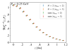
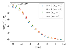
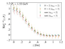
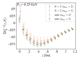
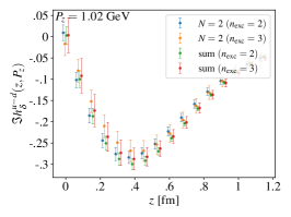
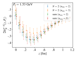
Figure 1: The Wilson-line length dependence of the (upper) real and (lower) imaginary parts of the isovector ground-state bare matrix elements from two-state and summation fits with $n_{\rm exc}=2,3$ for the three nonzero values of momentum considered (one for each column). The results shown are averaged with the negative $z$ fits.

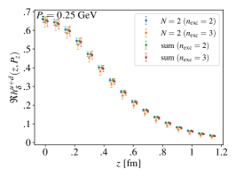
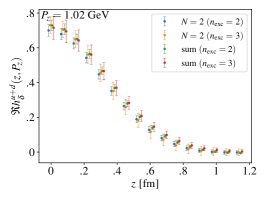
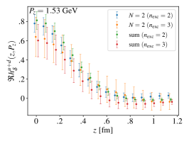
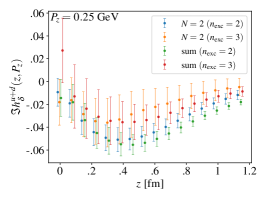
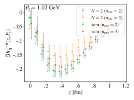
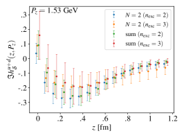
Figure 2: The same as Fig. 1, but for the isoscalar matrix elements.

We follow the standard approach for extracting the bare matrix elements, which begins by forming an appropriate ratio of the three-point to two-point correlation functions given by

$$R^{f}_{\delta}(P_{z},t_{\rm sep},t_{\rm ins},z)\equiv\frac{C^{\rm 3pt}_{\delta,f}(\vec{p}=P_{z}\hat{z},\vec{q}=0,t_{\rm sep},t_{\rm ins},z)}{C^{\rm 2pt}_{S_{x}}(\vec{p},t_{\rm sep})}.$$ (6)

The main reason for this choice is that it can be shown that

$$\lim_{t_{\rm ins},t_{\rm sep}\to\infty}R^{f}_{\delta}(P_{z},t_{\rm sep},t_{\rm ins},z)=h_{\delta;0,0}^{f}(z,P_{z}),$$ (7)

where $h_{\delta;0,0}^{f}(z,P_{z})$ is the desired bare ground-state matrix element. Since the values of $t_{\rm sep}$ considered here are not likely in the asymptotic region, we include the effects from the lowest $N$ states by substituting the spectral decompositions of the three- and two-point functions truncated at the $N$th state. After some algebra, we find

$$\begin{split}&R^{f}_{\delta}(P_{z},t_{\rm sep},t_{\rm ins},z;N)=\\ &\frac{\sum_{m,n=0}^{N-1}h^{\prime f}_{\delta;m,n}\prod_{l,k,r=1}^{m}e^{-\Delta_{l,l-1}t_{\rm sep}}e^{(\Delta_{k,k-1}-\Delta_{r,r-1})t_{\rm ins}}}{1+\sum_{i=1}^{N-1}r_{i}\prod_{j=1}^{i}e^{-\Delta_{j,j-1}t_{\rm sep}}},\end{split}$$ (8)

where $\Delta_{i,j}\equiv E_{i}-E_{j}$, $r_{i}\equiv|A_{\alpha}^{(i)}(P_{z})|^{2}/|A_{\alpha}^{(0)}(P_{z})|^{2}$, $A_{\alpha}^{(n)}(P_{z})\equiv\bra{\Omega}N_{\beta}\mathcal{P}_{\beta\alpha}\ket{n,P_{z}}$ ($\ket{\Omega}$ is the vacuum state and $\ket{n,P_{z}}$ is the $n$-th nucleon state with momentum $P_{z}$), and

$$h^{\prime f}_{\delta;m,n}\equiv\frac{A^{(m)}_{\alpha}(P_{z})A^{(n)}_{\alpha}(P_{z})^{\ast}h^{f}_{\delta;m,n}(z,P_{z})}{A^{(0)}_{\alpha}(P_{z})A^{(0)}_{\alpha}(P_{z})^{\ast}}.$$ (9)

The parameters $h^{\prime f}_{\delta;m,n}$ depend on $z$ and $P_{z}$, but this dependence is suppressed to save space. For convenience, we typically suppress the indices on the matrix elements when referring to the ground state matrix element (i.e. $h^{f}_{\delta}(z,P_{z})\equiv h^{f}_{\delta;0,0}(z,P_{z})$). As the excited-state matrix elements are never used, this should not cause any confusion. We fit the ratio of data in Eq. 6 to $R^{f}_{\delta}(P_{z},t_{\rm sep},t_{\rm ins},z;N)$, where $h^{\prime f}_{\delta;m,n}$, $\Delta_{i,j}$, and $r_{i}$ are the fit parameters. The parameters $\Delta_{i,j}$ and $r_{i}$ are priored using the fit results from the two-point functions (see Ref. Gao et al. (2023) for details). In this work, we only consider $N=1,2$, as our limited data tends to lead to unreliable fits when $N>2$.

In order to reduce the effects from unaccounted for excited-states as much as possible, we remove some of the data points nearest the sink and source times. We do this in a symmetric way, i.e. for each $t_{\rm ins}$ not included in the fit, we also do not include $t_{\rm sep}-t_{\rm ins}-1$. We define $n_{\rm exc}$ to be the number of insertion times removed on each side of the middle point for each $t_{\rm sep}$. Therefore, for each $t_{\rm sep}$, the insertion times included in the fit are $t_{\rm ins}\in[n_{\rm exc}+1,t_{\rm sep}-n_{\rm exc}-1]$. However, making $n_{\rm exc}$ too large can leave too little data left, and therefore we only consider $n_{\rm exc}\leq 3$. As described in our previous work of Ref. Gao et al. (2023), the two-point function fits show contributions from three states for $t_{\rm sep}\leq n_{\rm exc}+1$ requiring the use of an effective value for the prior on the gap $\Delta_{1,0}$ that takes into account effects from higher states. The specific value used for the prior on the gap comes from the two-state fit to the two-point function with the lower fit range $t_{\rm min}=n_{\rm exc}+1$.

As an additional consistency check on our fit results, we also make use of the summation method, which involves first summing $R^{f}_{\delta}(P_{z},t_{\rm sep},t_{\rm ins},z)$ over the subset $t_{\rm ins}\in[n_{\rm exc}+1,t_{\rm sep}-n_{\rm exc}-1]$ for each $t_{\rm sep}$

$$S^{f}_{\delta}(P_{z},t_{\rm sep},z;n_{\rm exc})\equiv\sum_{t_{\rm ins}=n_{\rm exc}+1}^{t_{\rm sep}-n_{\rm exc}-1}R^{f}_{\delta}(P_{z},t_{\rm sep},t_{\rm ins},z),$$ (10)

which reduces the leading contamination from excited states. The bare ground-state matrix element can then be extracted from a linear fit to the sum as

$$S^{f}_{\delta}(P_{z},t_{\rm sep},z;n_{\rm exc})=B_{0}+t_{\rm sep}h^{f}_{\delta}(z,P_{z}).$$ (11)

In Figs. 1 and 2, we show comparisons of the two-state and summation fit results for the isovector and isoscalar combinations, respectively, as a function of the Wilson line length for both $n_{\rm exc}=2$ and $3$. We see generally good agreement across these different fits, and, with the better data quality as compared to the unpolarized case, we choose our preferred fit as the two-state fit to the ratio Eq. 6 with $n_{\rm exc}=2$.

Several representative fits, all using our preferred fit strategy, are shown in App. B. There we include the fits to the zero-momentum local matrix elements, relevant for the tensor charge, in Fig. 18 for the isovector and isoscalar combinations. We also include various fits to the non-local matrix elements, relevant for information on the PDFs, in Figs. 19 and 20 for the isovector combination and in Figs. 21 and 22 for the isoscalar combination.

III.2 Tensor charge $g_{T}$

Although the focus of this work is based on the non-local matrix elements, we first turn our attention to the local ones which give us access to the nucleon tensor charge $g_{T}$. The bare matrix elements must be renormalized in a standard scheme (like $\overline{\text{MS}}$) in order to make comparisons with phenomenological results and other lattice determinations. The matrix elements are multiplicatively renormalizable, and we first determine the ratio of renormalization constants $Z_{T}/Z_{V}$ in the RI-MOM scheme which is then converted to $\overline{\text{MS}}$ at the scale $\mu=2$ GeV (see App. A for details). Then, using the ratio of bare charges $g_{T}^{\rm bare}/g_{V}^{\rm bare}$ along with the expectation of $Z_{V}g_{V}^{\rm bare}=1$, the renormalized tensor charge $g_{T}=Z_{T}g_{T}^{\rm bare}$ can be determined. Using our estimate for $Z_{T}/Z_{V}$, we find

$$\begin{split}g_{T}^{u-d}=1.05(2),\;\;\overline{\text{MS}}(\mu=2\;\text{GeV}),\\ g_{T}^{u+d}=0.64(2),\;\;\overline{\text{MS}}(\mu=2\;\text{GeV}).\end{split}$$ (12)

In Tab. 2, we show a comparison of our results to the other $N_{f}=2+1$ results given in the FLAG review 2021 Aoki et al. (2022).

	$g_{T}^{u-d}$	$g_{T}^{u}$	$g_{T}^{d}$
This work	1.05(2)	0.84(2)	-0.21(1)
NME Park et al. (2022)	0.95(5)(2)
RBC/UKQCD Abramczyk et al. (2020)	1.04(5)
Mainz Harris et al. (2019); Djukanovic et al. (2019)	$0.965(38)(^{13}_{41})$	0.77(4)(6)	-0.19(4)(6)
LHPC Hasan et al. (2019)	0.972(41)
JLQCD Yamanaka et al. (2018)	1.08(3)(3)(9)	0.85(3)(2)(7)	-0.24(2)(0)(2)
LHPC Green et al. (2012)	1.038(11)(12)
RBC/UKQCD Aoki et al. (2010)	0.9(2)

Table 2: Comparison of our extracted tensor charges with those in the FLAG review 2021 Aoki et al. (2022) with $N_{f}=2+1$. The results are ordered by year.

IV Mellin Moments from the Leading-twist OPE

We now move on to the extraction of the lowest few Mellin moments using the leading-twist OPE approximation. Here we avoid the need for the renormalization factors, which depend on the Wilson-line length $z$ and the lattice spacing $a$, by forming the renormalization-group invariant ratio Fan et al. (2020)

$$\mathcal{M}^{f/f^{\prime}}_{\delta}(\lambda,z^{2};P_{z}^{0})=\frac{h^{f}_{\delta}(z,P_{z})}{h^{f^{\prime}}_{\delta}(z,P_{z}^{0})}\big{/}\frac{h^{f}_{\delta}(0,P_{z})}{h^{f^{\prime}}_{\delta}(0,P_{z}^{0})},$$ (13)

where $\lambda\equiv zP_{z}$ is known as the Ioffe time. In the literature, this ratio is referred to as the Ioffe time pseudo-distribution (pseudo-ITD). In order to cancel the renormalization factors, the $z=0$ matrix elements are not necessary, but this choice is favorable in that it enforces a normalization and cancels correlations. In this work, we only consider the case with $P_{z}^{0}=0$, commonly referred to as the reduced pseudo-ITD Orginos et al. (2017); Joó et al. (2019, 2020); Bhat et al. (2021); Karpie et al. (2021); Egerer et al. (2021); Bhat et al. (2022). Additionally, since there are no gluons involved in the case of the transversity distributions, the leading-twist OPE expansion of the pseudo-ITD does not depend on the flavor combination $f^{\prime}$, even if $f\neq f^{\prime}$, and we, therefore, opt to omit the $f^{\prime}$ from our notation in order to not be overly cumbersome. In what follows, when extracting the isovector flavor combination, $f=f^{\prime}=u-d$, and for the isoscalar flavor combination, $f=u+d$ and $f^{\prime}=u-d$.

Then, using the leading-twist OPE approximation, we can write down the reduced pseudo-ITD as an expansion in Mellin moments

$$\begin{split}\mathcal{M}^{f}_{\delta}(\lambda,z^{2},P_{z}^{0}=0)=\sum_{n=0}\frac{C^{\delta}_{n}(\mu^{2}z^{2})}{C^{\delta}_{0}(\mu^{2}z^{2})}&\frac{(-i\lambda)^{n}}{n!}\frac{\braket{x^{n}}^{f}_{\delta}(\mu)}{\braket{x^{0}}^{f}_{\delta}(\mu)}\\ &+\mathcal{O}(\Lambda^{2}_{\rm QCD}z^{2}),\end{split}$$ (14)

where $C^{\delta}_{n}(\mu^{2}z^{2})$ are the Wilson coefficients for the transversity computed in the ratio scheme up to NLO in the strong coupling $\alpha_{s}(\mu)$, which at fixed order are given by Chen et al. (2016); Egerer et al. (2022)

$$\begin{split}C_{n,{\rm NLO}}^{\delta}(\mu^{2}z^{2})=1+\frac{\alpha_{s}(\mu)C_{F}}{2\pi}&\Bigg{[}2\ln(\frac{\mu^{2}z^{2}e^{2\gamma_{E}+1}}{4})\sum_{j=2}^{n+1}\frac{1}{j}\\ &-2\Bigg{(}\sum_{j=1}^{n}\frac{1}{j}\Bigg{)}^{2}-2\sum_{j=1}^{n}\frac{1}{j^{2}}\Bigg{]},\end{split}$$ (15)

$C_{F}=4/3$, and $\braket{x^{n}}^{f}_{\delta}(\mu)$ is the $n$th Mellin moment of the transversity PDF of flavor $f$ defined at the factorization scale $\mu$, i.e.

$$\braket{x^{n}}^{f}_{\delta}(\mu)=\int_{-1}^{1}\mathrm{d}x\,x^{n}\delta q^{f}(x,\mu),$$ (16)

where $\delta q^{f}(x,\mu)$ is the transversity PDF of a quark with flavor $f$ for $x\geq 0$ and of its antiquark for $x<0$. Estimates for the strong coupling itself are determined from Ref. Petreczky and Weber (2022), and we exclusively work at the scale $\mu=2$ GeV, resulting in $\alpha_{s}(\mu=2$ GeV$)=0.2930$. Further, we also consider the effects from target mass corrections (TMCs), which can be incorporated with the following substitution

$$\braket{x^{n}}^{f}_{\delta}\to\braket{x^{n}}^{f}_{\delta}\sum_{k=0}^{n/2}\frac{(n-k)!}{k!(n-2k)!}\bigg{(}\frac{m^{2}_{N}}{4P^{2}_{z}}\bigg{)}^{k}.$$ (17)

As the Wilson coefficients are all real, it is clear from Eq. 14 that the real and imaginary parts of the reduced pseudo-ITD, $\mathcal{M}_{\delta}^{f}(\lambda,z^{2},0)$, can be written solely in terms of the even and odd moments, respectively. Therefore, we choose to separately fit the real and imaginary parts of the reduced pseudo-ITD to

$$\begin{split}\real\mathcal{M}^{f}_{\delta}&(\lambda,z^{2},P_{z}^{0}=0)=\\ &\sum_{n=0}^{\lfloor N_{\rm max}/2\rfloor}\frac{C^{\delta}_{2n}(\mu^{2}z^{2})}{C^{\delta}_{0}(\mu^{2}z^{2})}\frac{(-i\lambda)^{2n}}{(2n)!}\braket{x^{2n}}^{\prime f}_{\delta},\\ \imaginary\mathcal{M}^{f}_{\delta}&(\lambda,z^{2},P_{z}^{0}=0)=\\ &\sum_{n=1}^{\lceil N_{\rm max}/2\rceil}\frac{C^{\delta}_{2n-1}(\mu^{2}z^{2})}{C^{\delta}_{0}(\mu^{2}z^{2})}\frac{(-i\lambda)^{2n-1}}{(2n-1)!}\braket{x^{2n-1}}^{\prime f}_{\delta},\end{split}$$ (18)

respectively, where the reduced moments $\braket{x^{n}}^{\prime f}_{\delta}\equiv\braket{x^{n}}^{f}_{\delta}/\braket{x^{0}}^{f}_{\delta}$ with $n>0$ are the fit parameters. The $n=0$ reduced moment is identically one, which is enforced explicitly in the fit. Additionally, $g_{T}^{f}\equiv\braket{x^{0}}^{f}_{\delta}$, which implies that the reduced moments are the original moments in units of the tensor charge, and we express all results as such.

We start the analysis as before in Ref. Gao et al. (2023) by first assessing the validity of the leading-twist approximation (i.e. how important are the $\mathcal{O}(\Lambda^{2}_{\rm QCD}z^{2})$ corrections which are ignored). To this end, we perform fits to Eq. 18 at only a single value for $z^{2}$ (referred to as a fixed-$z^{2}$ analysis) and look for any dependence of the extracted moments on the specific value of $z^{2}$. Observing little or no dependence on $z^{2}$ would suggest that the higher-twist contributions are negligible within our statistics and that the leading-twist approximation is valid.

As $z$ increases, the higher-moment terms in Eq. 14 begin to become important. We can determine when these higher-moment terms are expected to be non-negligible by using the leading-twist OPE with the moments extracted from the global analysis of JAM3D-22 Gamberg et al. (2022). We found that including two $n\neq 0$ moments in the OPE for both the real and imaginary parts is necessary for $z>4a\sim 0.304$ fm, and that a third $n\neq 0$ moment becomes necessary for $z>8a\sim 0.608$ fm. However, using only one value of $z^{2}$ allows for up to two moments to be fit to both the real and imaginary data, as the number of non-zero $P_{z}$ considered is three. Therefore, for the fixed-$z^{2}$ analysis, the largest value of $z$ used is $z=8a$ and we use two moments in the fits when $z>4a$.

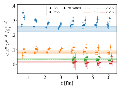
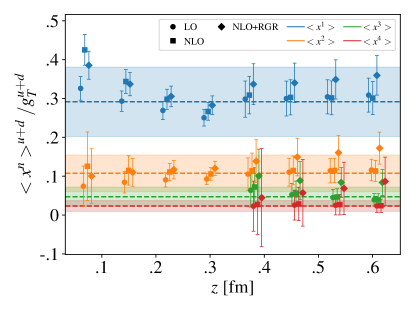
Figure 3: Results for the lowest four Mellin moments of the (upper) isovector and (lower) isoscalar PDF as a function of $z$ from fits of the reduced pseudo-ITD at fixed $z$ with $n_{z}\in[1,4,6]$ to the leading-twist OPE using LO, fixed-order NLO, and NLO+RGR Wilson coefficients evaluated at $\mu=2$ GeV, all of which include TMCs. Only the first two moments are extracted for $z\leq 4a$. The horizontal dashed lines and bands correspond to the central values and errors, respectively, of the moments extracted from the global analysis of JAM3D-22 Gamberg et al. (2022) defined at the scale $Q=2$ GeV.

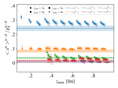
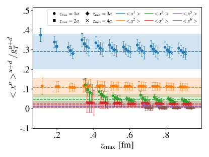
Figure 4: Results for the lowest four Mellin moments of the (upper) isovector and (lower) isoscalar PDF from uncorrelated fits of the reduced pseudo-ITD to the leading-twist OPE as a function of $z_{\rm max}$, with $z\in[z_{\rm min},z_{\rm max}]$ and $n_{z}\in[1,4,6]$. The results use the fixed-order NLO Wilson coefficients evaluated at $\mu=2$ GeV and include TMCs. Only the first two moments are considered for $z_{\rm max}\leq 4a$. The next two moments, $\braket{x^{3}}$ and $\braket{x^{4}}$ are included for $4a<z_{\rm max}\leq 8a$. And, two more moments, $\braket{x^{5}}$ and $\braket{x^{6}}$ are included for $z_{\rm max}>8a$. The horizontal dashed lines are the same as in Fig. 3.

Our results for the fixed-$z^{2}$ analysis for both the isovector and isoscalar combinations are show in Fig. 3. All results shown always include TMCs. Initially, we only considered the LO and fixed-order NLO Wilson coefficients in the analysis. However, the fixed-order NLO results show significant $z$ dependence for $\braket{x}$ at small values of $z$. This is not completely unexpected, as discretization errors Gao et al. (2020) and large logs can be significant for small values of $z$, see Appendix B in Ref. Gao et al. (2022b). Note, however, in that work, the analysis was done for the pion PDF, where the large logs become important at somewhat smaller $z$ compared to the range of $z$ where we see strong dependence here. To better understand the effects of large logs for the transversity PDF of the proton, we also use the NLO Wilson coefficients combined with renormalization group resummation (RGR) at next-to-leading logarithm (NLL) accuracy, given by

$$\begin{split}&C^{\delta}_{n,{\rm NLO+RGR}}(\mu^{2}z^{2})=C^{\delta}_{n,{\rm NLO}}(\mu_{0}^{2}z^{2})\\ &\;\;\;\;\;\times e^{-\frac{\gamma_{n}^{(1)}\textup{ln}\frac{a_{s}(\mu)}{a_{s}(\mu_{0})}}{\beta_{0}}-\frac{(-\beta_{1}\gamma_{n}^{(1)}+\beta_{0}\gamma_{n}^{(2)})\textup{ln}\frac{\beta_{0}+\beta_{1}a_{s}(\mu)}{\beta_{0}+\beta_{1}a_{s}(\mu_{0})}}{\beta_{0}\beta_{1}}},\end{split}$$ (19)

where $a_{s}=\alpha_{s}/(2\pi)$, $\beta_{n}$ is the $n$th order coefficient of the $\beta$ function, and $\gamma_{n}^{(1)}$ and $\gamma_{n}^{(2)}$ are the anomalous dimensions of the $n$th moments Vogelsang (1998); Ji et al. (2022). The RGR evolve the running coupling $\alpha_{s}$ from the physical scale $\mu_{0}=2e^{-\gamma_{E}}/z$ to the factorization scale $\mu$. As can be seen from Fig. 3, the use of the NLO+RGR Wilson coefficients produces results mostly consistent with the NLO case at small $z$. This suggests the significant $z$ dependence at small $z$ is mainly a discretization effect rather than due to large logs.

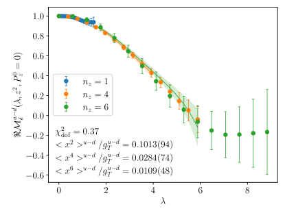
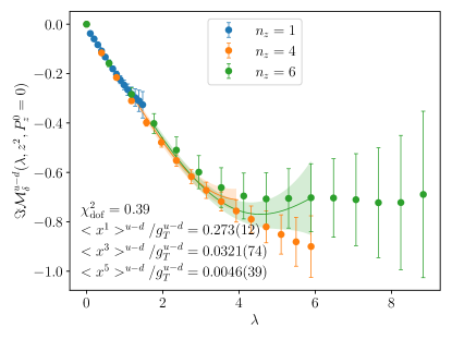
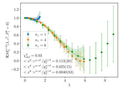
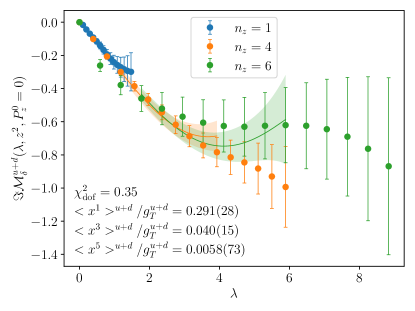
Figure 5: The (left) real and (right) imaginary parts of the (upper) isovector and (lower) isoscalar reduced pseudo-ITD for the three momentum used in this work. The data come from our preferred fit strategy described in Sec. III.1. The fit ranges used are $z\in[3a,10a]$. The shaded bands correspond to the fits using the leading-twist OPE with fixed-order NLO Wilson coefficients and TMCs evaluated at $\mu=2$ GeV and including three moments in both the real and imaginary parts.

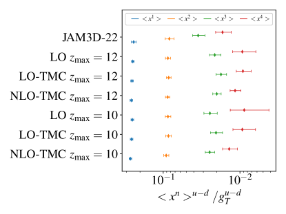
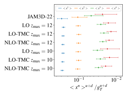
Figure 6: Summary plots of our extracted (left) isovector and (right) isoscalar moments from the leading-twist OPE approximation evaluated at $\mu=2$ GeV for various fitting strategies compared to the results from JAM3D-22 Gamberg et al. (2022) defined at the scale $Q=2$ GeV. Two $z_{\rm max}$ are considered, as well as Wilson coefficients at LO and fixed-order NLO.

Next, we move on to including a range of values of $z$ in our fits, considering various ranges $z\in[z_{\rm min},z_{\rm max}]$. With the extra data, we can include an extra moment in the fits for $z>8a$. The results for both the isovector and isoscalar moments are shown in Fig. 4. Given the small effect from the RGR which also becomes unstable when $a_{s}(\mu_{0})$ runs close to the Landau pole, we opt to use the fixed-order NLO Wilson coefficients, and also always include TMCs for the final results. There is some dependence on the choice of $z_{\rm min}$, as expected from the fixed-$z^{2}$ analysis results, however it is rather mild. Our preferred fit range is $z\in[3a,10a]$, which removes most of the effects from discretization errors and large logs at small $z$ and keeps $z_{\rm max}$ small enough to likely keep higher-twist contributions negligible. The results of these preferred fits are shown in Fig. 5. Finally, we show a summary of the results from different strategies and their comparison to JAM3D-22 Gamberg et al. (2022) in Fig. 6.

It is interesting to note the rather good agreement with the global analysis from JAM3D-22, especially for the lowest two moments, whereas we found tension for the lowest non-trivial moment in the unpolarized case Gao et al. (2023). However, comparing the matrix elements presented here versus those from the unpolarized ones, there is some hint of smaller excited-state contamination in the matrix elements of this work, which may be responsible for the better agreement.

V PDF from leading-twist OPE: DNN reconstruction

V.1 Method

It has been shown that we can extract the Mellin moments of transversity PDFs by applying the OPE formula to the ratio-scheme renormalized matrix elements, model independently. Limited by the finite $\lambda=zP_{z}$, the lattice data is only sensitive to the first few moments while the higher ones are factorially suppressed. As a result, to predict the $x$ dependence of the PDFs, one needs to introduce additional prior knowledge or a reasonable choice of model. Commonly used models are usually of the form

$$q(x)=Ax^{\alpha}(1-x)^{\beta}(1+\textup{sub-leading~{}terms}),$$ (20)

which is inspired by the end-point behavior of the PDFs. However, the sub-leading terms may play an important role, particularly in moderate regions of $x$, and one may find reasonable models for the sub-leading terms that give acceptable fits to the data. But, unless the data is precise, the model could introduce an uncontrolled bias. The use of a deep neural network (DNN) is a flexible way to maximally avoid any model bias — but cannot remove the bias entirely, as a nueral network is still a model — which is capable of approximating any functional form given a complicated enough network structure. As proposed in Ref. Gao et al. (2023), we parametrize the PDFs by,

$$q(x;\alpha,\beta,\bm{\theta})\equiv Ax^{\alpha}(1-x)^{\beta}[1+\epsilon(x)\sin({f_{\rm DNN}(x,\bm{\theta})})],$$ (21)

where $f_{\textup{DNN}}(x,\bm{\theta})$ is a DNN multistep iterative function, constructed layer by layer. The initial layer consists of a single node, denoted as $a_{1}^{1}$, which represents the input variable $x$. Subsequently, in the hidden layers, a linear transformation is performed using the equation:

$$z_{i}^{(l)}=b_{i}^{(l)}+\sum_{j}W_{ij}^{(l)}a_{j}^{(l-1)}.$$ (22)

Here, $z_{i}^{(l)}$ is the intermediate result obtained by adding the bias term $b_{i}^{(l)}$ to the sum of the weighted inputs from the previous layer, represented by $W_{ij}^{(l)}a_{j}^{(l-1)}$. Following this linear transformation, a nonlinear activation function $\sigma^{(l)}(z_{i}^{(l)})$ is applied, and the resulting output serves as the input to the next layer, represented by $a_{i}^{(l)}$. We specifically employed the exponential linear unit activation function $\sigma_{\textsf{elu}}(z)=\theta(-z)(e^{z}-1)+\theta(z)z$. Lastly, the final layer generates the output $f_{\text{DNN}}(x,\bm{\theta})$, which is subsequently utilized to evaluate $q(x;\alpha,\beta,\mathbf{\theta})$. The lower indices $i=1,...,n^{(l)}$ are used to identify specific nodes within the $l$th layer, where $n^{(l)}$ denotes the number of nodes in the $l$th layer. The upper indices, enclosed in parentheses, $l=1,...,N$, are employed to indicate the individual layers, where $N$ corresponds to the number of layers, representing the depth of the DNN. The parameters of the DNN, namely the biases $b_{i}^{(l)}$ and weights $W_{ij}^{(l)}$, represented by $\bm{\theta}$, are subject to optimization (training) by minimizing the loss function defined as

$$\begin{split}J(\bm{\theta})\equiv\frac{\eta}{2}\bm{\theta}\cdot\bm{\theta}+\frac{1}{2}\chi^{2}(\bm{\theta},\alpha,\beta,...).\end{split}$$ (23)

The first term in the loss function serves the purpose of preventing overfitting and ensuring that the function represented by the DNN remains well-behaved and smooth. The details of the $\chi^{2}$ function can be found in the appendix of Ref. Gao et al. (2023). Due to the limited statistics, a simple network structure such as $\{1,16,16,1\}$ (indicating the number of nodes in each layer) is sufficient to provide a smooth approximation of the sub-leading contribution. In practice, we experimented with different values of $\eta$ ranging from $10^{0}$ to $10^{-2}$ and considered network structures of sizes $\{1,16,16,1\}$, $\{1,16,16,16,1\}$, and $\{1,32,32,1\}$. However, the results remained consistent across these variations. Therefore, we opted for $\eta=0.1$ and selected a DNN structure with four layers, including the input and output layers, specified as $\{1,16,16,1\}$.

To balance the model bias and data precision, the contribution of the DNN is limited by $|\epsilon(x)\sin(f_{\rm DNN})|\lesssim\epsilon(x)$, which can be fully removed by setting $\epsilon(x)=0$. It is also possible to control the size of the DNN parametrized sub-leading contribution at each specific $x$. However, in this work, given the limited statistics, we simply fix $\epsilon(x)$ to be a small constant, e.g. $0.1$.

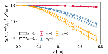
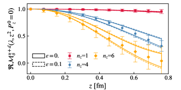
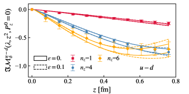
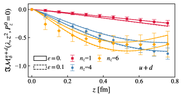
Figure 7: The DNN training results using the (left) isovector and (right) isoscalar reduced pseudo-ITD matrix elements in the range $z\in[2a,10a]$ for the (upper) real part and (lower) imaginary part (lower panel) are shown. The results using $\epsilon=0$ and $\epsilon=0.1$ are shown as the solid and dotted curves, respectively.

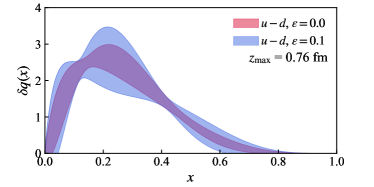
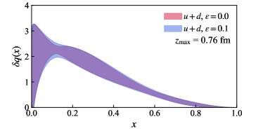
Figure 8: The DNN represented PDFs using the matrix elements in the range $z\in[2a,10a]$ for the (upper) isovector and (lower) isoscalar cases are shown. The results with $\epsilon=0$ and $\epsilon=0.1$ are shown as the red and blue bands, respectively.

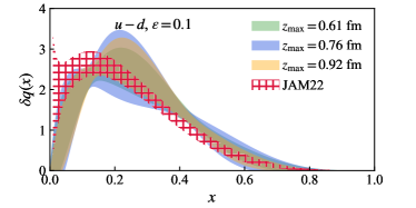
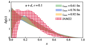
Figure 9: The DNN represented PDFs using the matrix elements in the range $z\in[2a,z_{\rm{max}}]$ for the (upper) isovector and (lower) isoscalar cases are shown. For comparison, we also show the global analysis results from JAM3D-22 Gamberg et al. (2022).

V.2 DNN represented PDF

To train the PDFs, we re-write the short distance factorization as,

$$\tilde{h}^{f}_{\delta}(z,P_{z},\mu)=\int_{-1}^{1}d\alpha\,\mathcal{C}^{\delta}(\alpha,\mu^{2}z^{2})\,\int_{-1}^{1}dy\,e^{-iy\alpha\lambda}\delta q^{f}(y,\mu),$$ (24)

where the renormalized matrix elements $\tilde{h}^{f}_{\delta}(z,P_{z},\mu)$ are directly connected to the $x$-dependent PDFs $\delta q^{f}(x,\mu)$, and $\mathcal{C}^{\delta}(\alpha,\mu^{2}z^{2})$ can be determined from the Wilson coefficients $C_{n}^{\delta}(\mu^{2}z^{2})$ Izubuchi et al. (2018); Ji et al. (2022). In this section we use the NLO fixed-order Wilson coefficients. In our case, the real and imaginary parts of the reduced pseudo-ITD $\mathcal{M}^{\frac{f}{f^{\prime}}}_{\delta}(\lambda,z^{2},P_{z}^{0}=0)$ are related to $\delta q^{f,-}(x)$ and $\delta q^{f,+}(x)$, defined as

$$\begin{split}&\delta q^{f,-}(x)\equiv\delta q^{f}(x)-\delta q^{\bar{f}}(x),\\ &\delta q^{f,+}(x)\equiv\delta q^{f}(x)+\delta q^{\bar{f}}(x),\end{split}$$ (25)

in the region $x\in[0,1]$ and where $\delta q^{f}(x)$ and $\delta q^{\bar{f}}(x)$ are the quark and anti-quark transversity distributions of flavor $f$, respectively. However, as observed in the literature Egerer et al. (2022); Yao et al. (2022), with the current lattice accuracy, the anti-quark distributions are mostly consistent with zero. We therefore ignore the anti-quark contribution and fit the real and imaginary parts together to $\delta q^{f}(x;\alpha,\beta,\bm{\theta})=\delta q^{f,-}(x)=\delta q^{f,+}(x)$.

We use the matrix elements in the range $z\in[2a,z_{\rm max}]$ for the parameter training, skipping $z=a$ in order to avoid the most serious discretization effects. In Fig. 7, we show the fit results for $z_{\rm max}=10a$ with $\epsilon=0$ and $\epsilon=0.1$ which both lead to a good description of the data. The corresponding PDFs are shown in Fig. 8, and the results from $\epsilon=0.1$ exhibit slightly larger errors but mostly overlap with the $\epsilon=0$ case. It is evident that the effects of the DNN were minimal which is likely a result of the limited statistics. We anticipate the DNN playing a more significant role when more precise data becomes available. In what follows, we use the results with $\epsilon=0.1$.

The short distance factorization could suffer from power corrections at large values of $z^{2}$. To check this, we vary the $z_{\rm max}$ used to train the PDFs to investigate such systematic errors. As shown in Fig. 9, by slightly increasing $z_{\rm max}$, the results do not change significantly within the large errors, suggesting that higher-twist effects are less important compared to the statistics of our data. For comparison, we also show the most recent global analysis results from JAM3D-22 Gamberg et al. (2022), and overall agreement is observed.

VI $x$-space Matching

We now move on to our final method for extracting information on the transversity PDF. This method utilizes LaMET to match the quasi-PDF — determined from the Fourier transform of hybrid-renormalized matrix elements — to the light-cone PDF.

VI.1 Hybrid renormalization

It is well known that the bare matrix elements can be multiplicatively renormalized by removing the linear divergence originating from the Wilson line self energy and the overall logarithmic divergence

$$h^{f}_{\delta}(z,P_{z})=Z_{T}(a)e^{-\delta m(a)z}e^{-\bar{m}_{0}z}\tilde{h}_{\delta}^{f}(z,P_{z}),$$ (26)

where $\tilde{h}_{\delta}^{f}$ is the renormalized matrix element, $\delta m(a)$ contains the Wilson-line self-energy linear UV divergences, $Z_{T}(a)$ contains the logarithmic UV divergences, and $\bar{m}_{0}$ is used to fix the scheme dependence present in $\delta m(a)$. The Wilson-line self-energy divergence term $\delta m(a)$ can be extracted from physical matrix elements, like those involving Wilson loops. Here we use the value $a\delta m(a)=0.1597(16)$ determined from the static quark-antiquark potential taken from Refs Bazavov et al. (2014, 2016); Bazavov et al. (2018a, b); Petreczky et al. (2022). The scheme dependence in $\delta m(a)$ can be attributed to a renormalon ambiguity, but can be fixed to a particular scheme by appropriate determiation of $\bar{m}_{0}$ Gao et al. (2022a); Zhang et al. (2023), and here we choose the $\overline{\rm MS}$ scheme. Our strategy for determining $\bar{m}_{0}$ is to compare the $P_{z}=0$ bare matrix elements $h_{\delta}^{f}(z,P_{z}=0)$ to the Wilson coefficient $C_{0}^{\delta}(\mu^{2}z^{2})$ computed in the $\overline{\rm MS}$ scheme

$$h_{\delta}^{f}(z,P_{z}=0)=Z_{T}(a)e^{-\delta m(a)z}e^{-\bar{m}_{0}z}C_{0}^{\delta}(\mu^{2}z^{2}).$$ (27)

In order to remove $Z_{T}(a)$ and hopefully cancel some of the discretization effects, we next divide (27) by itself with $z$ shifted by one unit of the lattice spacing. Then, after rearranging, we arrive at

$$e^{a\delta m(a)}\frac{h^{f}_{\delta}(z,P_{z}=0,a)}{h^{f}_{\delta}(z-a,P_{z}=0,a)}=e^{-a\bar{m}_{0}}\frac{C_{0}^{\delta}(\mu^{2}z^{2})}{C_{0}^{\delta}(\mu^{2}(z-a)^{2})}.$$ (28)

Before proceeding, we must first discuss the specifics of the Wilson coefficents used.

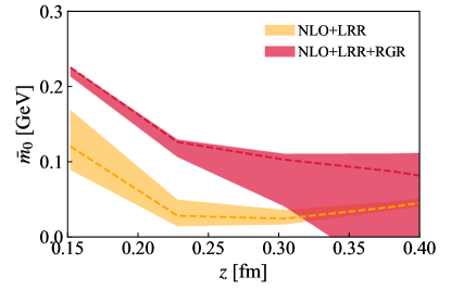
Figure 10: The $\bar{m}_{0}$ determined using NLO+LRR and NLO+LRR+RGR Wilson coefficients are shown. The bands come from the scale variation.

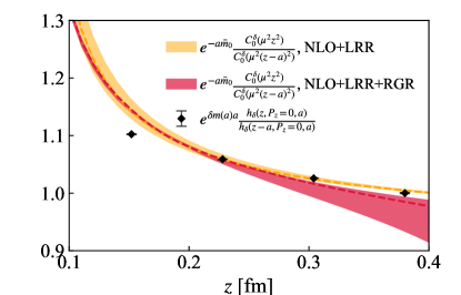
Figure 11: The ratio of $P_{z}=0$ matrix elements (black points) defined in Eq. (28) are shown. The bands are infered from the NLO+LRR and NLO+LRR+RGR Wilson coefficients respectively with scale variation.

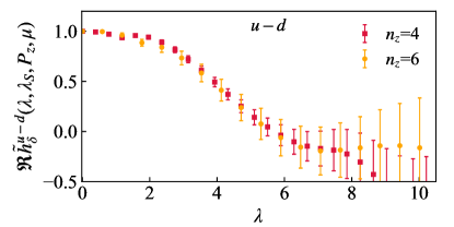
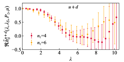
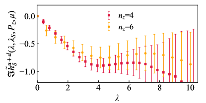
Figure 12: The (upper) real and (lower) imaginary parts of the renormalized matrix elements in the hybrid scheme for the (left) isovector and (right) isoscalar cobminations.

The renormalon ambiguity, by definition, is an artifact that arises from the summation prescription of the perturbative series in the QCD coupling $\alpha_{s}$. Therefore, we use the Wilson coefficients after leading renormalon resummation (LRR) given in Ref. Zhang et al. (2023) under the large-$\beta_{0}$ approximation by

$$\begin{split}C^{\delta}_{{0,\rm{LRR}}}(\alpha_{s}(\mu),&z^{2}\mu^{2})=\int_{0,{\rm PV}}^{\infty}d\omega e^{-\frac{4\pi\omega}{\beta_{0}\alpha_{s}(\mu)}}\frac{2C_{F}}{\beta_{0}}\frac{1}{\omega}\\ &\times\left[\frac{\Gamma(1-\omega)e^{\frac{5}{3}\omega}(z^{2}\mu^{2}/4)^{\omega}}{(1-2\omega)\Gamma(1+\omega)}-1\right].\end{split}$$ (29)

To be consistent with the known fixed-order Wilson coefficients at NLO, in practice, we use

$$\begin{split}&C_{0}^{\delta\prime}(\alpha_{s}(\mu),z^{2}\mu^{2})=C^{\delta}_{{0,\rm{LRR}}}(\alpha_{s}(\mu),z^{2}\mu^{2})\\ &+\left[C^{\delta}_{{0,\rm{NLO}}}(\alpha_{s}(\mu),z^{2}\mu^{2})-C^{\delta}_{{0,\rm{LRR,NLO}}}(\alpha_{s}(\mu),z^{2}\mu^{2})\right]\end{split}$$ (30)

where the $C^{\delta}_{{0,\rm{LRR,NLO}}}$ is the NLO expansion of $C^{\delta}_{{0,\rm{LRR}}}$ and the fixed-order NLO Wilson coefficient is given by

$$\begin{split}C^{\delta}_{{0,\rm{NLO}}}(\alpha_{s}(\mu),z^{2}\mu^{2})=1+\frac{\alpha_{s}(\mu)}{2\pi}C_{F}\left[2\ln(\frac{\mu^{2}z^{2}e^{2\gamma_{E}}}{4})+2\right].\end{split}$$ (31)

In addition, we can also resum the large logarithms $\ln(\mu^{2}z^{2}e^{2\gamma_{E}}/4)$ by the renormalization group resummation (RGR) Gao et al. (2021). Using these coefficients, the $\bar{m}_{0}$ determined using Eq. (28) are shown in Fig. 10 as a function of $z$. The bands of NLO+LRR come from the scale variation of $\mu$ in the Wilson coefficients by a factor of $\sqrt{2}$. When using RGR, the running coupling is evolved from the physical scale $\mu_{0}=2ke^{-\gamma_{E}}/z$ to the factorization scale $\mu$ Gao et al. (2021); Holligan et al. (2023). And we vary $k\in[1/\sqrt{2},1,\sqrt{2}]$ to estimate the scale uncertainty. It can be observed that the scale uncertainties in the RGR case are smaller at small $z$, benefiting from the resummation, while they become larger at large $z$ as they become close to the Landau pole. In addition, plateaus can be observed after $z\geq 3a\sim 0.228$ fm when the discretization effects become negligible, though the uncertainty bands for the NLO+LRR+RGR case are larger with the running coupling when $z>0.25$ fm. To avoid discretization effects at small $z$ and the Landau pole at large $z$, we choose values at $z=3a$ which give $\bar{m}_{0}=28(2)$ MeV and $129(2)$ MeV for NLO+LRR and NLO+LRR+RGR cases, respectively. In Fig. 11, we show the data points defined on the left-hand side of Eq. 28 using the computed matrix elements and $\delta m(a)$, along with the ratios defined on the right-hand side of Eq. 28 using $\bar{m}_{0}$ chosen above and Wilson coefficients at NLO+LRR (orange bands) and NLO+LRR+RGR (red bands).

The hybrid scheme renormalized matrix elements are given by

$$\begin{split}\tilde{h}^{f}_{\delta}(\lambda,\lambda_{s}&,P_{z},\mu)=\theta(z_{s}-z)\frac{h^{f}_{\delta}(z,P_{z},a)}{h^{f}_{\delta}(z,0,a)}\\ &+\theta(z-z_{s})\frac{h^{f}_{\delta}(z,P_{z},a)}{h^{f}_{\delta}(z_{s},0,a)}e^{(\delta m(a)+\bar{m}_{0})(z-z_{s})},\end{split}$$ (32)

with $z_{s}=3a$. In Fig. 12 we show the hybrid renormalized matrix elements for the isovector case (left panels) and isoscalar case (right panels) for momenta $n_{z}=4,6$. It can be seen that the large momentum matrix elements show a slow $P_{z}$ evolution and a good scaling in $\lambda$ within the statistical errors, suggesting we have good convergence in momentum.

VI.2 Extrapolation to large $\lambda$

Due to the finite extent of the lattice, one can only calculate the matrix elements up to some maximum $\lambda_{\rm max}\equiv z_{\rm max}P_{z}^{\rm max}$. Further, the signal deteriorates as $\lambda$ is increased. This poses a problem, as the matrix elements need to be Fourier transformed to obtain the quasi-PDF, and truncating the integral will lead to unphysical oscillations in the resulting quasi-PDF. Therefore, we choose to perform an extrapolation of the data to infinity before performing the Fourier transform. In practice, we estimate the Fourier transform with a discrete sum up to some value $\lambda_{L}=z_{L}P_{z}$ at which point an integral of the extrapolated function takes over. There are a few considerations when deciding upon an appropriate value for $\lambda_{L}$. In this work, we choose a value in the region where either the signal is no longer reliable or the values of the matrix elements are nearly consistent with zero. As in our previous work in Ref. Gao et al. (2023), the extrapolation itself is done by performing a fit in this region using the exponential decay model

$$\frac{Ae^{-m_{\rm eff}\lambda/P_{z}}}{|\lambda|^{d}},$$ (33)

where the fit parameters are constrained by $m_{\rm eff}>0.1$ GeV, $A>0$, and $d>0$. Using this constraint on $m_{\rm eff}$ helps to ensure the extrapolation falls off at a reasonable rate and does not significantly change the results in the regions of $x$ for which we trust the LaMET procedure. A detailed derivation which motivates the use of this model can be found in App. B of Ref. Gao et al. (2022a). Results of the extrapolation fits for the largest two momenta are shown in Fig. 13.

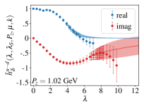
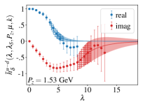
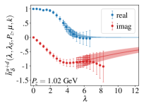
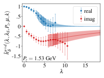
Figure 13: The (upper) isovector and (lower) isoscalar hybrid renormalized matrix elements with (left) $P_{z}=4\frac{2\pi}{L}$ and (right) $P_{z}=6\frac{2\pi}{L}$. The hatches show the range of data used for the fit to the extrapolation model and the bands are the result of that fit starting from $\lambda_{L}$. The hybrid renormalized data makes use of the NLO+LRR+RG Wilson coefficients computed at $\mu_{0}=2e^{-\gamma_{E}}/z$ (i.e. $k=1$) and subsequently evolved to $\mu=2$ GeV.

VI.3 The quasi-PDF from a Fourier transform

The quasi-PDF is defined as the Fourier transform of the renormalized matrix elements

$$\delta\tilde{q}^{f}(y,z_{s},P_{z},\mu)=\int\frac{dzP_{z}}{2\pi}e^{iyP_{z}z}\tilde{h}^{f}_{\delta}(z,z_{s},P_{z},\mu),$$ (34)

and is the LO approximation to the light-cone PDF within the LaMET framework. To perform this integral, we first exploit the symmetry of the renormalized matrix elements about $z=0$, i.e. $\tilde{h}^{f}_{\delta}(z,z_{s},P_{z},\mu)=\tilde{h}^{f}_{\delta}(-z,z_{s},P_{z},\mu)^{\ast}$, to rewrite the integral only over positive $z$

$$\begin{split}\delta\tilde{q}^{f}(y,z_{s},P_{z},\mu)=&\int_{0}^{\infty}\frac{dzP_{z}}{\pi}\real\tilde{h}^{f}_{\delta}(z,z_{s},P_{z},\mu)\cos(zP_{z}y)\\ -\int_{0}^{\infty}&\frac{dzP_{z}}{\pi}\imaginary\tilde{h}^{f}_{\delta}(z,z_{s},P_{z},\mu)\sin(zP_{z}y).\end{split}$$ (35)

Finally, we split the integrals up into two regions: i) $0\leq z\leq z_{L}$ where the integral is performed via a sum over the lattice data for $\tilde{h}^{f}_{\delta}(z,z_{s},P_{z},\mu)$ and ii) $z_{L}<z<\infty$ where the integral is performed using the resulting extrapolation for $\tilde{h}^{f}_{\delta}(z,z_{s},P_{z},\mu)$

$$\begin{split}\delta\tilde{q}^{f}&(y,z_{s},P_{z},\mu)=\\ &\Bigg{[}\sum_{z=0}^{z_{L}^{\rm re}/a}\frac{z_{L}^{\rm re}P_{z}}{\pi N_{z_{L}}^{\rm re}}+\int_{z_{L}^{\rm re}}^{\infty}\frac{dzP_{z}}{\pi}\Bigg{]}\real\tilde{h}^{f}_{\delta}(z,z_{s},P_{z},\mu)\cos(zP_{z}y)\\ -&\Bigg{[}\sum_{z=0}^{z_{L}^{\rm im}/a}\frac{z_{L}^{\rm im}P_{z}}{\pi N_{z_{L}}^{\rm im}}+\int_{z_{L}^{\rm im}}^{\infty}\frac{dzP_{z}}{\pi}\Bigg{]}\imaginary\tilde{h}^{f}_{\delta}(z,z_{s},P_{z},\mu)\sin(zP_{z}y),\end{split}$$ (36)

where $z_{L}^{\rm re}$ and $z_{L}^{\rm im}$ are the values of $z$ in which the extrapolation integral takes over for the real and imaginary parts of $\tilde{h}^{f}_{\delta}(z,z_{s},P_{z},\mu)$, respectively, and $N^{\rm re/im}\equiv z_{L}^{\rm re/im}/a+1$.

VI.4 Matching to the light-cone PDF

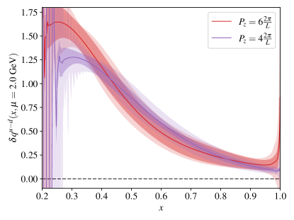
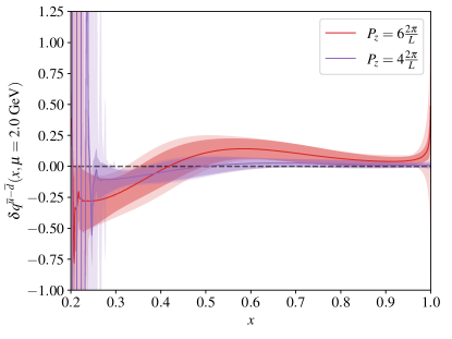
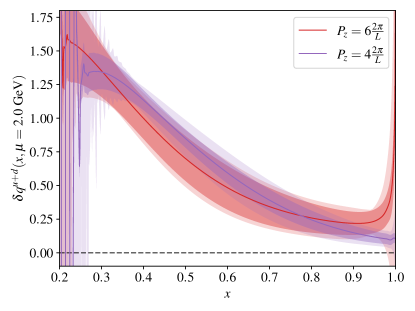
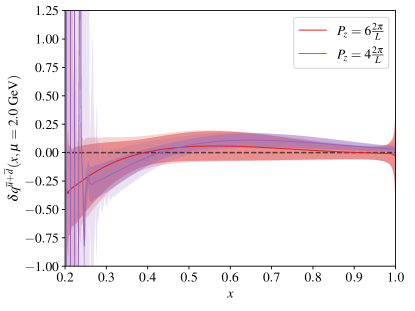
Figure 14: The $P_{z}$ dependence for the (upper) isovector and (lower) isoscalar (left) quark and (right) antiquark NLO+LRR+RGR light-cone transversity PDF $\delta q^{f}(x,\mu)$. The darker bands are the statistical errors when setting $k=1$ and the lighter bands are the additional systematic errors associated with scale variations by additionally using $k=1/\sqrt{2}$ and $k=\sqrt{2}$.

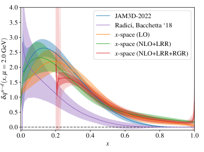
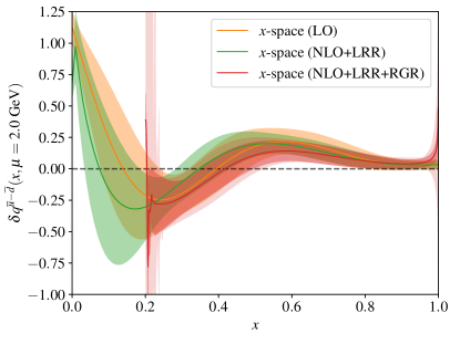
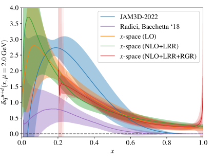
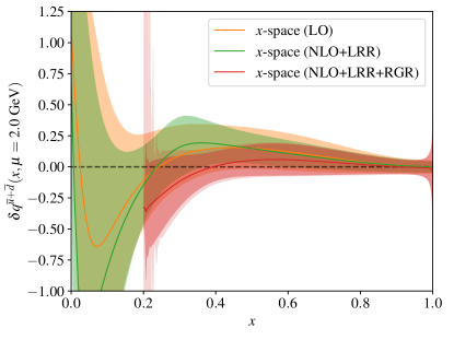
Figure 15: The (upper) isovector and (lower) isoscalar (left) quark and (right) antiquark transversity PDFs at LO, NLO+LRR, and NLO+LRR+RGR using the largest momentum $P_{z}=6\frac{2\pi}{L}$ and compared with the global analysis from JAM3D-22 Gamberg et al. (2022) and Radici, Bacchetta Radici and Bacchetta (2018) which are performed at LO. The darker bands for the NLO+LRR+RGR results are the statistical errors when setting $k=1$ and the lighter bands are the additional systematic errors associated with scale variations by additionally using $k=1/\sqrt{2}$ and $k=\sqrt{2}$.

The final step in obtaining the light-cone PDF from the quasi-PDF is to match them perturbatively in $\alpha_{s}(\mu)$ as

$$\begin{split}\delta q^{f}(x,\mu)&=\int^{\infty}_{-\infty}\frac{d{y}}{|y|}\mathcal{C}^{-1}_{\delta}\left(\frac{x}{y},\frac{\mu}{yP_{z}},|y|\lambda_{s}\right)\delta\tilde{q}^{f}(y,z_{s},P_{z},\mu)\\ &\phantom{==}+\mathcal{O}\left(\frac{\Lambda_{\rm QCD}^{2}}{x^{2}P_{z}^{2}},\frac{\Lambda_{\rm QCD}^{2}}{(1-x)^{2}P_{z}^{2}}\right)\\ &\equiv\mathcal{C}^{-1}_{\delta}\left(\frac{x}{y},\frac{\mu}{yP_{z}},|y|\lambda_{s}\right)\otimes\delta\tilde{q}^{f}(y,z_{s},P_{z},\mu)\\ &\phantom{==}+\mathcal{O}\left(\frac{\Lambda_{\rm QCD}^{2}}{x^{2}P_{z}^{2}},\frac{\Lambda_{\rm QCD}^{2}}{(1-x)^{2}P_{z}^{2}}\right),\end{split}$$ (37)

where $\mathcal{C}^{-1}_{\delta}(\frac{x}{y},\frac{\mu}{yP_{z}},|y|\lambda_{s})$ is the inverse of the perturbative matching kernel for the transversity distribution, and the notation $\otimes$ is used as short-hand for the integral. One caveat of this method is that the leading power corrections to the matching can be seen to be enhanced when $x$ is near 0 or 1. Therefore, we must be careful to estimate the range in $x$ in which these power corrections become significant and hence spoil the matching procedure.

To see how we obtain the the inverse matching kernel, we start with the perturbative expansion of the matching kernel itself

$$\begin{split}\mathcal{C}_{\delta}\left(\frac{x}{y},\frac{\mu}{yP_{z}},|y|\lambda_{s}\right)=\delta&\left(\frac{x}{y}-1\right)\\ &+\sum_{n=1}^{\infty}\alpha_{s}^{n}\mathcal{C}^{(n)}_{\delta}\left(\frac{x}{y},\frac{\mu}{yP_{z}},|y|\lambda_{s}\right),\end{split}$$ (38)

where only the NLO Wilson coefficients are known, i.e. we have only $\mathcal{C}^{(1)}_{\delta}(\frac{x}{y},\frac{\mu}{yP_{z}},|y|\lambda_{s})$ Xiong et al. (2014); Liu et al. (2018); Alexandrou et al. (2018); Ji et al. (2022). Next, by imposing the definition of the inverse matching kernel

$$\mathcal{C}^{-1}_{\delta}\left(\frac{x}{z},\frac{\mu}{zP_{z}},|z|\lambda_{s}\right)\otimes\mathcal{C}_{\delta}\left(\frac{z}{y},\frac{\mu}{yP_{z}},|y|\lambda_{s}\right)=\delta\left(\frac{x}{y}-1\right),$$ (39)

we find

$$\begin{split}\mathcal{C}^{-1}_{\delta}&\left(\frac{x}{y},\frac{\mu}{yP_{z}},|y|\lambda_{s}\right)=\delta\left(\frac{x}{y}-1\right)\\ &-\alpha_{s}\mathcal{C}^{(1)}\left(\frac{x}{y},\frac{\mu}{yP_{z}},|y|\lambda_{s}\right)+\mathcal{O}(\alpha_{s}^{2}).\end{split}$$ (40)

As done in our previous work Ref. Gao et al. (2023), we approximate the integration by defining the integral on a finite-length grid which can be represented via matrix multiplication with a matching matrix $C^{\delta}_{xy}$ to obtain the light-cone PDF at NLO as

$$\delta q^{f}(x,\mu)=\delta\tilde{q}^{f}(x,\mu)-\delta y\sum_{y}C^{\delta,{\rm NLO}}_{xy}\tilde{q}^{f}(y,\mu),$$ (41)

where $\delta y=0.001$ is the grid size used for the integration.

For the matching coefficients themselves, we also implement LRR and RGR, where the RGR involves running the coupling from the physical scale $\mu_{0}$ with three choices of $k\in[1/\sqrt{2},1,\sqrt{2}]$ to $\mu=2$ GeV which allows for assessing the systematics due to scale variation.

VI.5 Results

As a first check regarding the significance of the power corrections, we show the momentum dependence of the NLO light-cone PDFs for both the isovector and isoscalar flavor combinations using our largest two momenta in Fig. 14. There we see a relatively mild momentum dependence, which is expected given the observed momentum convergence in the renormalized matrix elements shown in Fig. 12.

Finally, using the largest available momentum of $P_{z}=6\frac{2\pi}{L}$, in Fig. 15 we show the quark and antiquark transversity distributions for both the isovector and isoscalar flavor combinations compared to the global analysis from JAM3D-22 Gamberg et al. (2022) and Radici, Bacchetta Radici and Bacchetta (2018) which are both performed at LO.

There are a few things to note about these results. First, recall that the global analysis and our DNN results both assume the anti-quark distribution to be zero. Our $x$-space matching results in this section favor this assumption, at least when using an NLO matching kernel.

Further, recall that power corrections in the light-cone matching lead to a breakdown of the formalism when $x\sim 0,1$. However, the RGR results also breakdown at small $x$, as seen by the onset of oscillations near $x\sim 0.2$, already giving a natural boundary for where we no longer trust the results.

VII Conclusions

In this paper we have presented various extractions of the transversity isovector and isoscalar quark PDFs, and their lowest few moments, of the proton from lattice QCD using a physical pion mass. This work is a continuation towards the ultimate goal of uncovering the full structure of the proton from first principles. Additionally, the matrix elements needed in this work also allow an estimate of the tensor charge $g_{T}$ to be extracted, and our results show reasonable agreement with other lattice extractions, as shown in Tab. 2. However, our calculations are performed at a single value of the lattice spacing, and for the isoscalar case we neglected the disconnected diagrams.

Regarding the transversity isovector and isoinglet PDFs, in our first method, we utilized the leading-twist OPE expansion of the reduced pseudo-ITD to extract the first few Mellin moments. We found excellent agreement with the global analysis from JAM3D-22 for the lowest two moments and minor tensions for the next two moments. Higher moments could not be reliably extracted. Next, we used the pseudo-PDF approach, based on short-distance factorization, to extract an $x$-dependent PDF and utilized a deep neural network to overcome the inverse problem while remaining as unbiased as possible. We saw some mild tension with the results from JAM3D-22 for a few small ranges of $x$ but otherwise mostly saw agreement. Finally, we used the quasi-PDF approach, based on LaMET, to calculate the $x$-dependence PDF from hybrid-scheme renormalized matrix elements. For this we found reasonably good agreement with JAM3D-22 in the moderate region of $x$, but there is significant tension with the results from Radici, Bacchetta.

A number of systematics are being ignored here and are left for future work. These include the use of a single lattice spacing, NNLO corrections in $\alpha_{s}$, power corrections from the use of finite momentum, and isoscalar disconnected diagrams. We can address the expected significance of these systematics, and we have good reason to expect their effects to be rather small. Regarding the NNLO corrections, we saw in Fig. 15 the NLO corrections were relatively mild in the middle $x$ regions, suggesting that NNLO corrections will be quite small as seen for the unpolarized proton distribution in our previous work Gao et al. (2023). And, for the disconnected diagrams, we discussed earlier the expectation that the effects of these diagrams for local operator matrix elements would be smaller than the statistical error based on the study done in Refs. Bhattacharya et al. (2015a, b). Further, in our study of the unpolarized proton distribution Gao et al. (2023), we saw no evidence of convergence in the momentum used. However, as seen in Fig. 14, the convergence in momentum is much more convincing for the transversity distribution.

Appendix A Renormalization constant $Z_{T}$ in RI-MOM scheme

Here we discuss the extraction of the renormalization constant $Z_{T}$ in the RI-MOM scheme and its subsequent conversion to the $\overline{\text{MS}}$ scheme at the scale $\mu=2$ GeV. The method starts by calculating matrix elements between off-shell quark states with lattice momenta

$$ap_{\mu}=\frac{2\pi}{L_{\mu}}(n_{\mu}+\frac{1}{2}\delta_{\mu 0}),$$ (42)

where $L_{\mu}$ is the size of the lattice in the $\mu$th direction, $n_{\mu}\in\mathbb{Z}$, and $\mu=0$ is the temporal direction. These matrix elements are computed in the Landau gauge. The renormalization point is given by $(ap_{R})^{2}\equiv\sum_{\mu=0}^{3}\sin^{2}(ap_{\mu})$, which is inspired by the lattice dispersion relation and helps to reduce discretization errors. Our results for $Z_{T}$ are shown in Fig. 16.

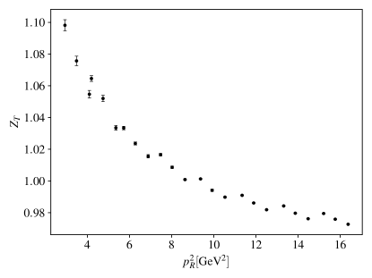
Figure 16: The tensor current renormalization factor $Z_{T}$ as a function of the RI-MOM momentum $p_{R}$.

There is a significant dependence on $p_{R}^{2}$ caused by non-perturbative associated with condensates and discretization errors that can be clearly seen from the “fishbone” structure at large $p_{R}^{2}$. We had difficulty appropriately modeling these effects and instead chose to form ratios of $Z_{T}/Z_{V}$ in an attempt to cancel them as much as possible, similar to what was done in Ref. Bhattacharya et al. (2014). We then use the conversion factor from RI-MOM to $\overline{\text{MS}}$ for the tensor current computed in Ref. Gracey (2003) to three loops. The resulting renormalization factors are then in the $\overline{\text{MS}}$ scheme at the scale $\mu^{2}=p_{R}^{2}$, and thus we evolve them to the same scale using the evolution function computed at two loops in Ref. Chetyrkin (1997). We evolve $Z_{T}$ to the scale $\mu=2$ GeV, as this is a commonly used scale for reporting results of nucleon charges. The resulting ratio $Z_{T}/Z_{V}$ after conversion to $\overline{\text{MS}}$ at $\mu=2$ GeV is then fit to

$$Z_{T}/Z_{V}+B/p_{R}^{2}+D_{1}p_{R}+D_{2}p_{R}^{2},$$ (43)

where last two terms incorporate discretization effects. In order to remove bias from our choice of fit, we consider six different variations of this fit form, corresponding to setting various terms to zero. Specifically, we consider a linear form (i.e. $D_{2}=0$), a quadratic form (i.e. $D_{1}=0$), and a linear+quadratic form (i.e. $D_{1}\neq 0$ and $D_{2}\neq 0$). Then for each of these three, we also consider fits in which $B$ is zero and non-zero. To further give variation to our fits, we use three ranges of the data. The first includes all but the smallest values of $p_{R}^{2}$, which is always left out. Then we consider removing more of the small $p_{R}^{2}$ data, and finally removing the largest $p_{R}^{2}$ data. This gives a total of 18 fits we consider. To give a final estimate, we simply take an AIC average over all fits, giving

$$Z_{T}/Z_{V}=1.050(17),\;\;\overline{\text{MS}}(\mu=2\;\text{GeV}).$$ (44)

The results of all these fits are shown in Fig. 17. This, rather conservative, method for estimating the systematic error is justified for this observable which is likely affected by large systematics.

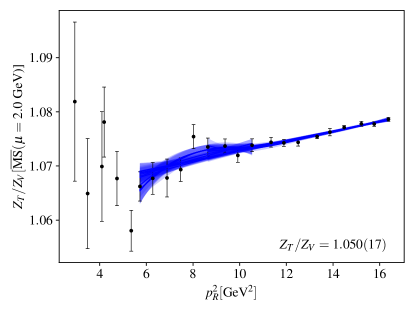
Figure 17: Ratio of the tensor to vector current renormalization factors $Z_{T}/Z_{V}$ as a function of the RI-MOM momentum $p_{R}$. The bands show the 18 different fits considered, all overlaid on top of one another. The AIC-averaged result final result for the ratio is given in the bottom right corner.

Appendix B Three-point function fits

Here we show a handful of fits to the ratios of three-point to two-point functions used in the main text. All of these fits utilize our preferred fit strategy, i.e. the two-state fit to the ratio $R_{\delta}$ in (6) with $n_{\rm exc}=2$, where $n_{\rm exc}$ is the number of data points nearest both the source and sink that are not included in the fit.

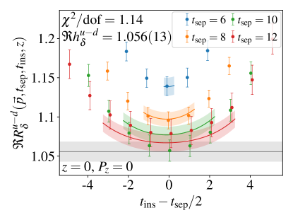
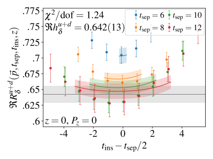
Figure 18: The real parts of the ratio of local (left) isovector and (right) isoscalar three-point to two-point functions for $P_{z}=0$. The $\chi^{2}/\textrm{dof}$ reported, estimate for the ground-state bare matrix element (also represented by a gray band), and $t_{\rm sep}$ fit bands come from the preferred fit strategy, i.e. the two-state fit to the ratio $R_{\delta}$ with $n_{\rm exc}=2$, where $n_{\rm exc}$ is the number of data points nearest both the source and sink that are not included in the fit. The range in $t_{\rm ins}$ of the $t_{\rm sep}$ bands covers the included data points in the fit.

The fits included here are to the local zero-momentum three to two-point function ratios, shown in Fig. 18, and several non-local three to two-point function ratios, shown in Figs. 19, 20, 21 and 22. These include both isovector and isoscalar combinations.

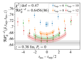
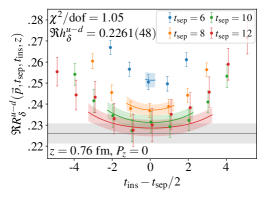
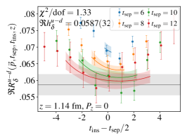
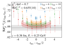
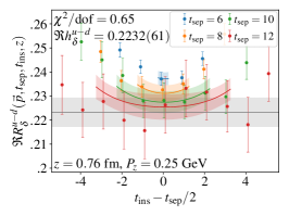
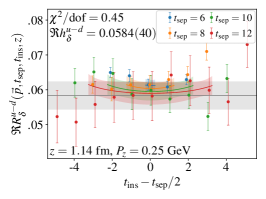
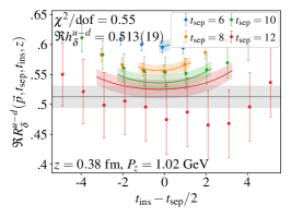
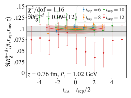
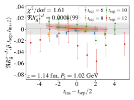
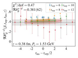
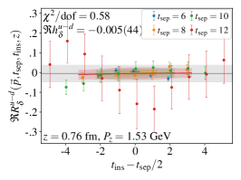
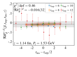
Figure 19: The real parts of the ratio of isovector three-point to two-point functions for all values of momentum (one for each row) and a few representative values of Wilson-line length $z$ (one for each column). The $\chi^{2}/\textrm{dof}$ reported, estimate for the ground-state bare matrix element (also represented by a gray band), and $t_{\rm sep}$ fit bands come from the preferred fit strategy, i.e. the two-state fit to the ratio $R_{\delta}$ with $n_{\rm exc}=2$, where $n_{\rm exc}$ is the number of data points nearest both the source and sink that are not included in the fit. The range in $t_{\rm ins}$ of the $t_{\rm sep}$ bands covers the included data points in the fit.

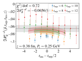
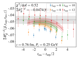
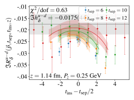
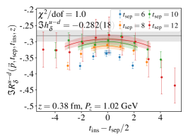
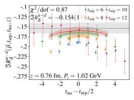
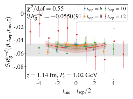
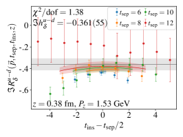
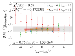
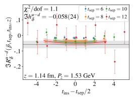
Figure 20: The same as Fig. 19, but for the imaginary parts. Additionally, the zero-momentum matrix elements are not shown, as these are all consistent with zero (as they are expected to be).

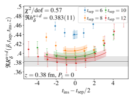
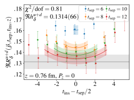
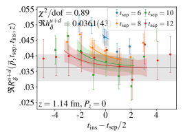
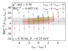
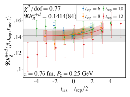
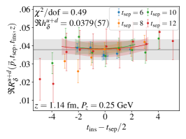
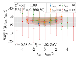
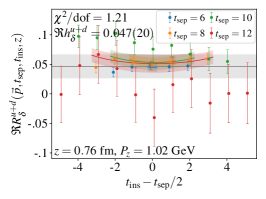
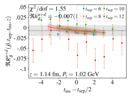
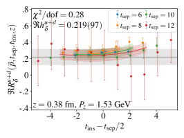
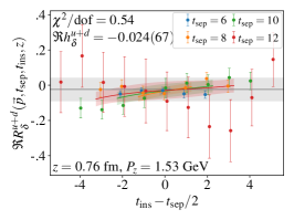
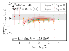
Figure 21: The same as Fig. 19, but for the isoscalar matrix elements.

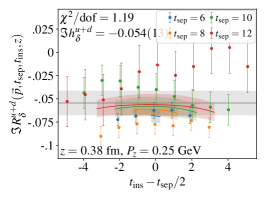
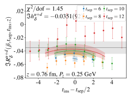
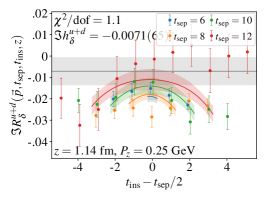
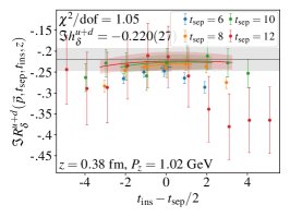
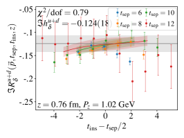
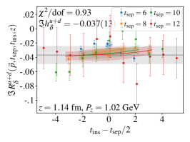
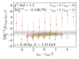
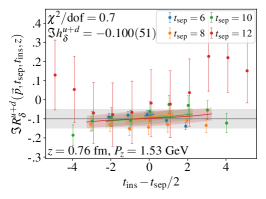
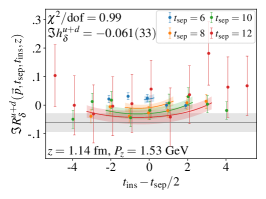
Figure 22: The same as Fig. 21, but for the imaginary parts. Additionally, the zero-momentum matrix elements are not shown, as these are all consistent with zero (as they are expected to be).

References

- Alekhin et al. (2017) S. Alekhin, J. Blümlein, S. Moch, and R. Placakyte, Phys. Rev. D 96, 014011 (2017), eprint 1701.05838.
- Hou et al. (2021) T.-J. Hou et al., Phys. Rev. D 103, 014013 (2021), eprint 1912.10053.
- Bailey et al. (2021) S. Bailey, T. Cridge, L. A. Harland-Lang, A. D. Martin, and R. S. Thorne, Eur. Phys. J. C 81, 341 (2021), eprint 2012.04684.
- Ball et al. (2022) R. D. Ball et al. (NNPDF), Eur. Phys. J. C 82, 428 (2022), eprint 2109.02653.
- Adolph et al. (2015) C. Adolph et al. (COMPASS), Phys. Lett. B 744, 250 (2015), eprint 1408.4405.
- Airapetian et al. (2020) A. Airapetian et al. (HERMES), JHEP 12, 010 (2020), eprint 2007.07755.
- Adolph et al. (2012) C. Adolph et al. (COMPASS), Phys. Lett. B 713, 10 (2012), eprint 1202.6150.
- Adolph et al. (2014) C. Adolph et al. (COMPASS), Phys. Lett. B 736, 124 (2014), eprint 1401.7873.
- Airapetian et al. (2008) A. Airapetian et al. (HERMES), JHEP 06, 017 (2008), eprint 0803.2367.
- Yang (2009) R. Yang (PHENIX), AIP Conf. Proc. 1182, 569 (2009).
- Fatemi (2012) R. Fatemi (STAR), AIP Conf. Proc. 1441, 233 (2012), eprint 1206.3861.
- Adamczyk et al. (2015) L. Adamczyk et al. (STAR), Phys. Rev. Lett. 115, 242501 (2015), eprint 1504.00415.
- Bacchetta et al. (2011) A. Bacchetta, A. Courtoy, and M. Radici, Phys. Rev. Lett. 107, 012001 (2011), eprint 1104.3855.
- Bacchetta et al. (2013) A. Bacchetta, A. Courtoy, and M. Radici, JHEP 03, 119 (2013), eprint 1212.3568.
- Anselmino et al. (2013) M. Anselmino, M. Boglione, U. D’Alesio, S. Melis, F. Murgia, and A. Prokudin, Phys. Rev. D 87, 094019 (2013), eprint 1303.3822.
- Kang et al. (2015) Z.-B. Kang, A. Prokudin, P. Sun, and F. Yuan, Phys. Rev. D 91, 071501 (2015), eprint 1410.4877.
- Martin et al. (2015) A. Martin, F. Bradamante, and V. Barone, Phys. Rev. D 91, 014034 (2015), eprint 1412.5946.
- Radici et al. (2015) M. Radici, A. Courtoy, A. Bacchetta, and M. Guagnelli, JHEP 05, 123 (2015), eprint 1503.03495.
- Anselmino et al. (2015) M. Anselmino, M. Boglione, U. D’Alesio, J. O. Gonzalez Hernandez, S. Melis, F. Murgia, and A. Prokudin, Phys. Rev. D 92, 114023 (2015), eprint 1510.05389.
- Kang et al. (2016) Z.-B. Kang, A. Prokudin, P. Sun, and F. Yuan, Phys. Rev. D 93, 014009 (2016), eprint 1505.05589.
- Radici et al. (2016) M. Radici, A. M. Ricci, A. Bacchetta, and A. Mukherjee, Phys. Rev. D 94, 034012 (2016), eprint 1604.06585.
- Lin et al. (2018) H.-W. Lin, W. Melnitchouk, A. Prokudin, N. Sato, and H. Shows, Phys. Rev. Lett. 120, 152502 (2018), eprint 1710.09858.
- Radici and Bacchetta (2018) M. Radici and A. Bacchetta, Phys. Rev. Lett. 120, 192001 (2018), eprint 1802.05212.
- Benel et al. (2020) J. Benel, A. Courtoy, and R. Ferro-Hernandez, Eur. Phys. J. C 80, 465 (2020), eprint 1912.03289.
- Anselmino et al. (2020) M. Anselmino, R. Kishore, and A. Mukherjee, Phys. Rev. D 102, 096012 (2020), eprint 2009.03148.
- D’Alesio et al. (2020) U. D’Alesio, C. Flore, and A. Prokudin, Phys. Lett. B 803, 135347 (2020), eprint 2001.01573.
- Cammarota et al. (2020) J. Cammarota, L. Gamberg, Z.-B. Kang, J. A. Miller, D. Pitonyak, A. Prokudin, T. C. Rogers, and N. Sato (Jefferson Lab Angular Momentum), Phys. Rev. D 102, 054002 (2020), eprint 2002.08384.
- Gamberg et al. (2022) L. Gamberg, M. Malda, J. A. Miller, D. Pitonyak, A. Prokudin, and N. Sato (Jefferson Lab Angular Momentum (JAM), Jefferson Lab Angular Momentum), Phys. Rev. D 106, 034014 (2022), eprint 2205.00999.
- Cocuzza et al. (2023a) C. Cocuzza, A. Metz, D. Pitonyak, A. Prokudin, N. Sato, and R. Seidl (JAM) (2023a), eprint 2306.12998.
- Cocuzza et al. (2023b) C. Cocuzza, A. Metz, D. Pitonyak, A. Prokudin, N. Sato, and R. Seidl (2023b), eprint 2308.14857.
- Dudek et al. (2012) J. Dudek et al., Eur. Phys. J. A 48, 187 (2012), eprint 1208.1244.
- Burkert et al. (2023) V. D. Burkert et al., Prog. Part. Nucl. Phys. 131, 104032 (2023), eprint 2211.15746.
- Cichy and Constantinou (2019) K. Cichy and M. Constantinou, Adv. High Energy Phys. 2019, 3036904 (2019), eprint 1811.07248.
- Zhao (2019) Y. Zhao, Int. J. Mod. Phys. A 33, 1830033 (2019), eprint 1812.07192.
- Radyushkin (2020) A. V. Radyushkin, Int. J. Mod. Phys. A 35, 2030002 (2020), eprint 1912.04244.
- Ji et al. (2021a) X. Ji, Y.-S. Liu, Y. Liu, J.-H. Zhang, and Y. Zhao, Rev. Mod. Phys. 93, 035005 (2021a), eprint 2004.03543.
- Constantinou (2021) M. Constantinou, Eur. Phys. J. A 57, 77 (2021), eprint 2010.02445.
- Constantinou et al. (2021) M. Constantinou et al., Prog. Part. Nucl. Phys. 121, 103908 (2021), eprint 2006.08636.
- Cichy (2022) K. Cichy, PoS LATTICE2021, 017 (2022), eprint 2110.07440.
- Ji (2013) X. Ji, Phys. Rev. Lett. 110, 262002 (2013), eprint 1305.1539.
- Ji (2014) X. Ji, Sci. China Phys. Mech. Astron. 57, 1407 (2014), eprint 1404.6680.
- Radyushkin (2017) A. V. Radyushkin, Phys. Rev. D 96, 034025 (2017), eprint 1705.01488.
- Orginos et al. (2017) K. Orginos, A. Radyushkin, J. Karpie, and S. Zafeiropoulos, Phys. Rev. D 96, 094503 (2017), eprint 1706.05373.
- Ji et al. (2017) X. Ji, J.-H. Zhang, and Y. Zhao, Nucl. Phys. B 924, 366 (2017), eprint 1706.07416.
- Radyushkin (2018) A. V. Radyushkin, Phys. Lett. B 781, 433 (2018), eprint 1710.08813.
- Izubuchi et al. (2018) T. Izubuchi, X. Ji, L. Jin, I. W. Stewart, and Y. Zhao, Phys. Rev. D 98, 056004 (2018), eprint 1801.03917.
- Ji (2022) X. Ji (2022), eprint 2209.09332.
- Holligan et al. (2023) J. Holligan, X. Ji, H.-W. Lin, Y. Su, and R. Zhang, Nucl. Phys. B 993, 116282 (2023), eprint 2301.10372.
- Chen et al. (2016) J.-W. Chen, S. D. Cohen, X. Ji, H.-W. Lin, and J.-H. Zhang, Nucl. Phys. B 911, 246 (2016), eprint 1603.06664.
- Alexandrou et al. (2018) C. Alexandrou, K. Cichy, M. Constantinou, K. Jansen, A. Scapellato, and F. Steffens, Phys. Rev. D 98, 091503 (2018), eprint 1807.00232.
- Liu et al. (2018) Y.-S. Liu, J.-W. Chen, L. Jin, R. Li, H.-W. Lin, Y.-B. Yang, J.-H. Zhang, and Y. Zhao (2018), eprint 1810.05043.
- Alexandrou et al. (2019) C. Alexandrou, K. Cichy, M. Constantinou, K. Hadjiyiannakou, K. Jansen, A. Scapellato, and F. Steffens, Phys. Rev. D 99, 114504 (2019), eprint 1902.00587.
- Alexandrou et al. (2021) C. Alexandrou, M. Constantinou, K. Hadjiyiannakou, K. Jansen, and F. Manigrasso, Phys. Rev. D 104, 054503 (2021), eprint 2106.16065.
- Yao et al. (2022) F. Yao et al. (Lattice Parton) (2022), eprint 2208.08008.
- Egerer et al. (2022) C. Egerer et al. (HadStruc), Phys. Rev. D 105, 034507 (2022), eprint 2111.01808.
- Constantinou and Panagopoulos (2017) M. Constantinou and H. Panagopoulos, Phys. Rev. D 96, 054506 (2017), eprint 1705.11193.
- Alexandrou et al. (2017) C. Alexandrou, K. Cichy, M. Constantinou, K. Hadjiyiannakou, K. Jansen, H. Panagopoulos, and F. Steffens, Nucl. Phys. B 923, 394 (2017), eprint 1706.00265.
- Chen et al. (2018) J.-W. Chen, T. Ishikawa, L. Jin, H.-W. Lin, Y.-B. Yang, J.-H. Zhang, and Y. Zhao, Phys. Rev. D 97, 014505 (2018), eprint 1706.01295.
- Stewart and Zhao (2018) I. W. Stewart and Y. Zhao, Phys. Rev. D 97, 054512 (2018), eprint 1709.04933.
- Ji et al. (2021b) X. Ji, Y. Liu, A. Schäfer, W. Wang, Y.-B. Yang, J.-H. Zhang, and Y. Zhao, Nucl. Phys. B 964, 115311 (2021b), eprint 2008.03886.
- Zhang et al. (2023) R. Zhang, J. Holligan, X. Ji, and Y. Su, Phys. Lett. B 844, 138081 (2023), eprint 2305.05212.
- Gao et al. (2023) X. Gao, A. D. Hanlon, J. Holligan, N. Karthik, S. Mukherjee, P. Petreczky, S. Syritsyn, and Y. Zhao, Phys. Rev. D 107, 074509 (2023), eprint 2212.12569.
- Gao et al. (2022a) X. Gao, A. D. Hanlon, S. Mukherjee, P. Petreczky, P. Scior, S. Syritsyn, and Y. Zhao, Phys. Rev. Lett. 128, 142003 (2022a), eprint 2112.02208.
- Gao et al. (2022b) X. Gao, A. D. Hanlon, N. Karthik, S. Mukherjee, P. Petreczky, P. Scior, S. Shi, S. Syritsyn, Y. Zhao, and K. Zhou (2022b), eprint 2208.02297.
- Follana et al. (2007) E. Follana, Q. Mason, C. Davies, K. Hornbostel, G. P. Lepage, J. Shigemitsu, H. Trottier, and K. Wong (HPQCD, UKQCD), Phys. Rev. D 75, 054502 (2007), eprint hep-lat/0610092.
- Bazavov et al. (2019) A. Bazavov et al., Phys. Rev. D 100, 094510 (2019), eprint 1908.09552.
- Hasenfratz and Knechtli (2001) A. Hasenfratz and F. Knechtli, Phys. Rev. D 64, 034504 (2001), eprint hep-lat/0103029.
- Bali et al. (2016) G. S. Bali, B. Lang, B. U. Musch, and A. Schäfer, Phys. Rev. D 93, 094515 (2016), eprint 1602.05525.
- Izubuchi et al. (2019) T. Izubuchi, L. Jin, C. Kallidonis, N. Karthik, S. Mukherjee, P. Petreczky, C. Shugert, and S. Syritsyn, Phys. Rev. D 100, 034516 (2019), eprint 1905.06349.
- Pochinsky (2008–present) A. Pochinsky, Qlua lattice software suite, https://usqcd.lns.mit.edu/qlua (2008–present).
- Clark et al. (2010) M. A. Clark, R. Babich, K. Barros, R. C. Brower, and C. Rebbi, Comput. Phys. Commun. 181, 1517 (2010), eprint 0911.3191.
- Babich et al. (2011) R. Babich, M. A. Clark, B. Joo, G. Shi, R. C. Brower, and S. Gottlieb, in SC11 International Conference for High Performance Computing, Networking, Storage and Analysis (2011), eprint 1109.2935.
- Shintani et al. (2015) E. Shintani, R. Arthur, T. Blum, T. Izubuchi, C. Jung, and C. Lehner, Phys. Rev. D 91, 114511 (2015), eprint 1402.0244.
- Bhattacharya et al. (2015a) T. Bhattacharya, V. Cirigliano, R. Gupta, H.-W. Lin, and B. Yoon, Phys. Rev. Lett. 115, 212002 (2015a), eprint 1506.04196.
- Bhattacharya et al. (2015b) T. Bhattacharya, V. Cirigliano, S. Cohen, R. Gupta, A. Joseph, H.-W. Lin, and B. Yoon (PNDME), Phys. Rev. D 92, 094511 (2015b), eprint 1506.06411.
- Aoki et al. (2022) Y. Aoki et al. (Flavour Lattice Averaging Group (FLAG)), Eur. Phys. J. C 82, 869 (2022), eprint 2111.09849.
- Park et al. (2022) S. Park, R. Gupta, B. Yoon, S. Mondal, T. Bhattacharya, Y.-C. Jang, B. Joó, and F. Winter (Nucleon Matrix Elements (NME)), Phys. Rev. D 105, 054505 (2022), eprint 2103.05599.
- Abramczyk et al. (2020) M. Abramczyk, T. Blum, T. Izubuchi, C. Jung, M. Lin, A. Lytle, S. Ohta, and E. Shintani, Phys. Rev. D 101, 034510 (2020), eprint 1911.03524.
- Harris et al. (2019) T. Harris, G. von Hippel, P. Junnarkar, H. B. Meyer, K. Ottnad, J. Wilhelm, H. Wittig, and L. Wrang, Phys. Rev. D 100, 034513 (2019), eprint 1905.01291.
- Djukanovic et al. (2019) D. Djukanovic, H. Meyer, K. Ottnad, G. von Hippel, J. Wilhelm, and H. Wittig, PoS LATTICE2019, 158 (2019), eprint 1911.01177.
- Hasan et al. (2019) N. Hasan, J. Green, S. Meinel, M. Engelhardt, S. Krieg, J. Negele, A. Pochinsky, and S. Syritsyn, Phys. Rev. D 99, 114505 (2019), eprint 1903.06487.
- Yamanaka et al. (2018) N. Yamanaka, S. Hashimoto, T. Kaneko, and H. Ohki (JLQCD), Phys. Rev. D 98, 054516 (2018), eprint 1805.10507.
- Green et al. (2012) J. R. Green, J. W. Negele, A. V. Pochinsky, S. N. Syritsyn, M. Engelhardt, and S. Krieg, Phys. Rev. D 86, 114509 (2012), eprint 1206.4527.
- Aoki et al. (2010) Y. Aoki, T. Blum, H.-W. Lin, S. Ohta, S. Sasaki, R. Tweedie, J. Zanotti, and T. Yamazaki, Phys. Rev. D 82, 014501 (2010), eprint 1003.3387.
- Fan et al. (2020) Z. Fan, X. Gao, R. Li, H.-W. Lin, N. Karthik, S. Mukherjee, P. Petreczky, S. Syritsyn, Y.-B. Yang, and R. Zhang, Phys. Rev. D 102, 074504 (2020), eprint 2005.12015.
- Joó et al. (2019) B. Joó, J. Karpie, K. Orginos, A. Radyushkin, D. Richards, and S. Zafeiropoulos, JHEP 12, 081 (2019), eprint 1908.09771.
- Joó et al. (2020) B. Joó, J. Karpie, K. Orginos, A. V. Radyushkin, D. G. Richards, and S. Zafeiropoulos, Phys. Rev. Lett. 125, 232003 (2020), eprint 2004.01687.
- Bhat et al. (2021) M. Bhat, K. Cichy, M. Constantinou, and A. Scapellato, Phys. Rev. D 103, 034510 (2021), eprint 2005.02102.
- Karpie et al. (2021) J. Karpie, K. Orginos, A. Radyushkin, and S. Zafeiropoulos (HadStruc), JHEP 11, 024 (2021), eprint 2105.13313.
- Egerer et al. (2021) C. Egerer, R. G. Edwards, C. Kallidonis, K. Orginos, A. V. Radyushkin, D. G. Richards, E. Romero, and S. Zafeiropoulos (HadStruc), JHEP 11, 148 (2021), eprint 2107.05199.
- Bhat et al. (2022) M. Bhat, W. Chomicki, K. Cichy, M. Constantinou, J. R. Green, and A. Scapellato, Phys. Rev. D 106, 054504 (2022), eprint 2205.07585.
- Petreczky and Weber (2022) P. Petreczky and J. H. Weber, Eur. Phys. J. C 82, 64 (2022), eprint 2012.06193.
- Gao et al. (2020) X. Gao, L. Jin, C. Kallidonis, N. Karthik, S. Mukherjee, P. Petreczky, C. Shugert, S. Syritsyn, and Y. Zhao, Phys. Rev. D 102, 094513 (2020), eprint 2007.06590.
- Vogelsang (1998) W. Vogelsang, Phys. Rev. D 57, 1886 (1998), eprint hep-ph/9706511.
- Ji et al. (2022) Y. Ji, F. Yao, and J.-H. Zhang (2022), eprint 2212.14415.
- Bazavov et al. (2014) A. Bazavov et al. (HotQCD), Phys. Rev. D 90, 094503 (2014), eprint 1407.6387.
- Bazavov et al. (2016) A. Bazavov, N. Brambilla, H. T. Ding, P. Petreczky, H. P. Schadler, A. Vairo, and J. H. Weber, Phys. Rev. D 93, 114502 (2016), eprint 1603.06637.
- Bazavov et al. (2018a) A. Bazavov, P. Petreczky, and J. H. Weber, Phys. Rev. D 97, 014510 (2018a), eprint 1710.05024.
- Bazavov et al. (2018b) A. Bazavov, N. Brambilla, P. Petreczky, A. Vairo, and J. H. Weber (TUMQCD), Phys. Rev. D 98, 054511 (2018b), eprint 1804.10600.
- Petreczky et al. (2022) P. Petreczky, S. Steinbeißer, and J. H. Weber, PoS LATTICE2021, 471 (2022), eprint 2112.00788.
- Gao et al. (2021) X. Gao, K. Lee, S. Mukherjee, C. Shugert, and Y. Zhao, Phys. Rev. D 103, 094504 (2021), eprint 2102.01101.
- Xiong et al. (2014) X. Xiong, X. Ji, J.-H. Zhang, and Y. Zhao, Phys. Rev. D 90, 014051 (2014), eprint 1310.7471.
- Lepage (2022a) P. Lepage, gplepage/lsqfit: lsqfit version 12.0.3 (2022a), https://github.com/gplepage/lsqfit.
- Lepage (2022b) P. Lepage, gplepage/gvar: gvar version 11.9.5 (2022b), https://github.com/gplepage/gvar.
- Hunter (2007) J. D. Hunter, Comput. Sci. Eng. 9, 90 (2007).
- Bhattacharya et al. (2014) T. Bhattacharya, S. D. Cohen, R. Gupta, A. Joseph, H.-W. Lin, and B. Yoon, Phys. Rev. D 89, 094502 (2014), eprint 1306.5435.
- Gracey (2003) J. A. Gracey, Nucl. Phys. B 662, 247 (2003), eprint hep-ph/0304113.
- Chetyrkin (1997) K. G. Chetyrkin, Phys. Lett. B 404, 161 (1997), eprint hep-ph/9703278.