Wavelet-based Ramsey magnetometry enhancement of a single NV center in diamond

Abstract

Nitrogen-vacancy (NV) centers in diamond constitute a solid-state nanosensing paradigm. Specifically for high-precision magnetometry, the so-called Ramsey interferometry is the prevalent choice where the sensing signal is extracted from time-resolved spin-state-dependent photoluminescence (PL) data. Its sensitivity is ultimately limited by the photon shot noise (PSN), which cannot be sufficiently removed by averaging or frequency filtering. Here, we propose Ramsey DC magnetometry of a single NV center enhanced by a wavelet-denoising scheme specifically tailored to suppress PSN. It simply operates as a post-processing applied on a collected PL time series. Our implementation is based on template margin thresholding which we computationally benchmark, and demonstrate its signal-to-noise-ratio improvement over the standard quantum limit by up to an order of magnitude for the case of limited-time-budget measurements.

I Introduction

Certain point defects embedded in a solid-state matrix can have optically addressable spin states [1]. Among these, the negatively charged nitrogen-vacancy (NV^-) center [2] is particularly favored with its long coherence time up to one second [3], rendering it apt for quantum sensing of fields [4, 5, 6], nanoscale magnetic field textures [7], strain [8], temperature [9, 10], rotation sensing [11], and biomedical applications [12, 13], as well as three-dimensional mapping of spinful ¹³C nuclei in proximity of the defect center [14, 15].

This initial success has spurred a strong incentive for ever-pushing the sensitivity limits of NV centers [16]. These involve experimental efforts like spin echo time enhancements in shallow NV^- [17], using excited-level anticrossing to enhance readout fluorescence contrast [18], or by boosting photon collection efficiency [19], spin to charge conversion [20, 21], charge noise suppression for achieving high optical coherence [22], nuclear spin polarization for high-field magnetometry [23], utilizing double-quantum transitions for doubling the effective gyromagnetic ratio [24, 25], to name just a few. Moreover, there are new sensing modalities such as ancilla-assisted repetitive readout [26, 27, 28], or involving proximal nuclear spins [29, 30, 31], covariance magnetometry for obtaining spatiotemporal correlations with two NV^- center [32], cascading weak measurements into a projective one [33], in addition to so-called post-processing approaches like Bayesian phase estimation protocols proposed for increasing dynamic range and sensitivity [34, 35, 36].

The dominant readout noise in such sensors is primarily mitigated by averaging over uncorrelated repeated measurements which attains the so-called standard quantum limit (SQL) as a consequence of the central limit theorem [37]. This essentially amounts to low-pass filtering of the noise from the sensing signal. A commonly held view to surpass SQL is to harness quantum resources with the most powerful one being entanglement, albeit being very challenging as it makes it prone to faster decoherence [38]. On the other hand, it has been asserted that SQL can be beaten by purely classical means as long as coherence in the system is preserved during averaging [39, 40]. As a matter of fact, employing noise filtering has proven to be quite potent, as exemplified in boosting gate fidelity to above the surface code error correction limit [41] or coherence protection of NV qubit by deep-learning to improve sensitivity [42].

Most adversely, NV-center sensors suffer from the photon shot noise (PSN), which has non-stationary temporal characteristics [38, 16] lowering the effectiveness of conventional frequency filtering. In this respect, more advanced signal processing has been advocated for improving the low signal-to-noise ratio (SNR) of time-resolved spin-dependent fluorescence, to which we will simply refer as photoluminescence (PL) [43]. Serving for the same purpose an underutilized tool is the wavelet analysis. As a well-established technique [44], it is previously used in this context for the fast detection of temporal magnetic fields [45], and for resolving spatial positioning of spinful nuclei around central spin [46], and most recently for extraction of both spatially and temporally correlated noise in a two-spin-qubit silicon metal-oxide-semiconductor device [47].

In this work, our aim is to put forward the efficacy of wavelet-enhanced Ramsey magnetometry of a single NV center, allowing us to develop a time- and frequency-tailored wavelet denoising scheme against PSN. Thus, it does not necessitate any quantum resource, and per se, is a post-processing applied over the PL time series that is routinely collected by these sensors. We show that the wavelet-based, so-called, template margin thresholding (TMT) method can improve the SNR of PL data significantly in slope detection points and can be highly desirable for limited integration time applications.

This paper is organized as follows. In Sec. II we describe the spin Hamiltonian and dephasing mechanism of a single NV-center. This is followed by Sec. III in which wavelet transform and TMT filter are introduced. Section IV highlights parameters considered alongside with the chosen metrics that underpin the TMT-enhancement quantitatively. In Sec. V, we present our numerical simulation results regarding the performance of the TMT filter under different PL settings. Next, in Sec. VI we provide our conclusions and future prospects for TMT, and Appendix contains some basic terminology and information about wavelets.

II Model Hamiltonian and dephasing time

The ultimate limitation to sensitivity is born out of decoherence due to the interaction with the environmental ¹³C nuclei, as quantified by the dephasing time $T_{2}^{*}$. Choosing the computational $z$-quantization basis parallel to the NV-axis, the general spin Hamiltonian can be categorized into three parts,

$$H=H_{\text{NV}}+H_{\text{int}}+H_{\text{env}},$$ (1)

where $H_{\text{NV}}$, represents the NV-center, $H_{\text{int}}$ describes the interaction between the NV-center and the environment, and $H_{\text{env}}$ is the Hamiltonian of the spin bath. Under external magnetic field $B_{0}$, its explicit form becomes [48],

$$H_{\text{NV}}/\hbar =DS_{z}^{2}-\gamma_{e}\vec{B}_{0}\cdot\vec{S}+\epsilon(S_{x}^{2}-S_{y}^{2})$$

$$+\gamma_{N}\vec{B}_{0}\cdot\vec{I}+\vec{I}\cdot\mathbb{P}\cdot\vec{I}+\vec{S}\cdot\mathbb{A}\cdot\vec{I},$$ (2)

$$H_{\text{int}}/\hbar =\sum_{i=1}^{N}\vec{S}\cdot\mathbb{A}_{i}\cdot\vec{I}_{i},$$ (3)

$$H_{\text{env}}/\hbar =-\gamma_{c}\vec{B}_{0}\cdot\sum_{j=1}^{N}\vec{I}_{j}+\sum_{i<j}\vec{I}_{i}\cdot\mathbb{D}_{ij}\cdot\vec{I}_{j}$$ (4)

where, $D=2\pi\times 2.87$ GHz is zero-field splitting, $S_{n}$ ($I_{n}$) represents the electron (nitrogen) spin operator in the $\hat{n}$ direction, $\gamma_{e}=-2\pi\times 28.024$ GHz/T ($\gamma_{N}=2\pi\times 3.077$ MHz/T) is gyromagnetic ratio of electron (nitrogen), $\vec{B}$ is the external magnetic field, $\epsilon=2\pi\times 100$ kHz is strain induced transverse anisotropy term [49], $\mathbb{P}$ and $\mathbb{A}$ are quadrupolar and hyperfine interaction tensors, respectively. The subscripts in (3) and (4) represent the corresponding spinfull nuclear spin site, so that $\mathbb{A}_{i}$ refers to the hyperfine interaction tensor for the $i$th nuclear spin. In $H_{\text{env}}$, $\gamma_{c}=2\pi\times 10.708$ MHz/T is the gyromagnetic ratio of ¹³C, and $\mathbb{D}$ is the dipole-dipole interaction tensor.

With the large zero-field splitting, and assuming that $B_{0}$ is aligned with the NV axis, the non-secular terms in $\mathbb{A}_{i}$ interaction tensor can be dropped [50, 46]. We also note that the ¹³C spins that are in the vicinity of NV-defect ($<1$ nm) have non-vanishing Fermi-contact terms. It has been shown that they are not the main source of the dephasing mechanism, and since these fastly oscillating terms can be silenced by dynamical decoupling techniques [16], they can be safely ignored. For a single NV-center, since dephasing time $T_{2}^{*}$ highly depends on the hyperfine couplings and hence the spatial distribution of ¹³C nuclei [51, 50, 52], we consider randomly distributed 1100 ¹³C bath spins, which has approximately 1% natural abundance in diamond structure. To mimic the thermalized nuclear spin bath dynamics (i.e. with a joint density operator, $\rho\propto\otimes_{i}\hat{\mathcal{I}}_{i}$), we average out 1000 different initial nuclear spin realizations to calculate coherence of the central spin, under $B_{0}=40$ mT. With these parameters and via second-order generalized cluster correlation expansion (gCCE) [53, 54], we have extracted according to the expression $e^{-(t/T_{2}^{*})^{p}}$, the dephasing time, $T_{2}^{*}=3.9~{}\mu$s, and decay factor, $p=2$.

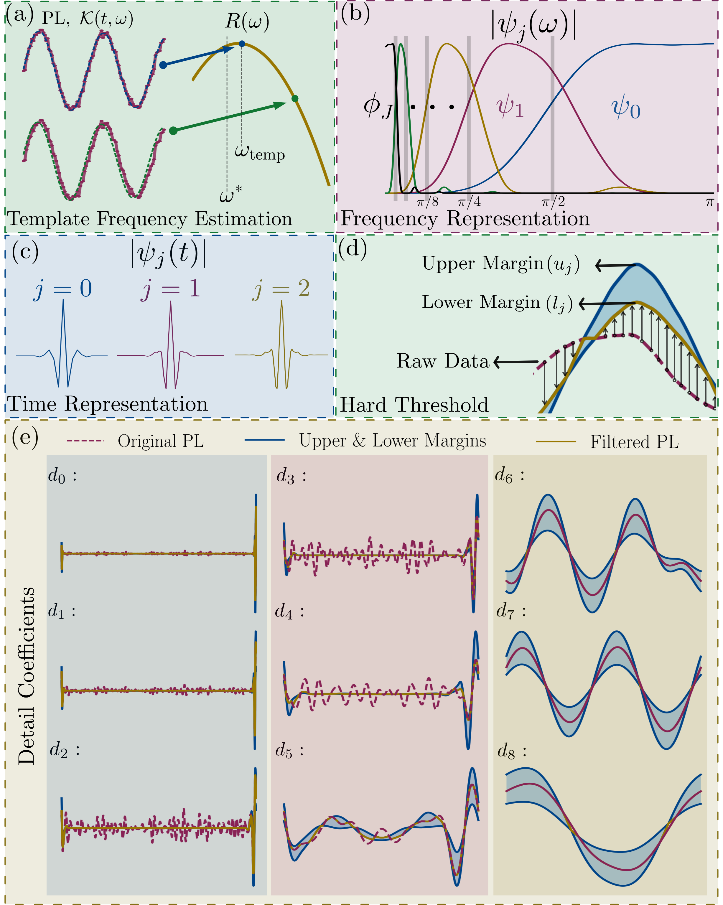
Figure 1: (a) Estimation of template frequency by means of Eq. $(\ref{xcorr})$. The red line represents PL collected between the time interval $[t_{i}=0.97~{}\mu$s, $t_{f}=1.75~{}\mu$s] with sampling frequency $f_{\text{sample}}\sim 128$ MHz and $M=25$K, blue and green lines are $\mathcal{K}(t,\omega)$ at different trial frequencies. The green line mismatches with the PL, whereas the blue line maximizes the $R(\omega)$ and is employed as template frequency. There is an offset between the true value ($\omega^{*}$) and the template ($\omega_{\text{temp}}$). (b) Frequency representation of biorthogonal 6.8 wavelet at different scales, $|\psi_{j}(\omega)|$, and father wavelet (scaling function) $|\phi_{J}|$. Each wavelet $\psi_{j}$ splits the remaining frequency axis into two and $\phi_{J}$ spans the low frequencies with the $\omega=0$ value to provide a compact representation of a given signal. (c) biorthogonal 6.8 wavelet at different scales in the time domain. (d) Representation of hard threshold (Eq. $(\ref{hard})$), blue line corresponds to upper and lower margins, red dashed and yellow lines indicate raw and filtered signal, respectively. (e) Enhancement of PL signal provided in (a) up to $d_{8}$.

III PSN tailored wavelet enhancement

III.1 Wavelet transform

The wavelet representation of a signal, $x(t)$ in terms of set of scaling ($\phi_{j,k}$) and wavelet functions ($\psi_{j,k}$) take the form

$$x(t)=\sum_{k=-\infty}^{\infty}c_{j_{0},k}\phi_{j_{0},k}(t)+\sum_{j=-\infty}^{j_{0}}\sum_{k=-\infty}^{\infty}d_{j,k}\psi_{j,k}(t),$$ (5)

where, their inner products $c_{j,k}=\langle x(t),\phi_{j,k}(t)\rangle$ and $d_{j,k}=\langle x(t),\phi_{j,k}(t)\rangle$ are called as an approximation and detail coefficients, respectively (see, Appendix for details). Instead of evaluating the approximation and detail coefficients with such inner products each time, the discrete wavelet transform (DWT) of $x(t)$ can be calculated by utilizing half-band-lowpass and half-band-bandpass filters recursively such that [55, 56],

$$c_{j,k} =\sum_{m}h_{0}(m-2k)c_{j-1,m},$$ (6)

$$d_{j,k} =\sum_{m}h_{1}(m-2k)c_{j-1,m},$$ (7)

where $h_{0}$ and $h_{1}$ are lowpass and highpass filter coefficients. DWT is an efficient method for signal decomposition yet, it suffers from time invariance due to downsampling. In this work, we use undecimated wavelet transform (UWT), also known as the stationary wavelet transform, which is a DWT without decimation.

III.2 Template margin thresholding

Under an external magnetic field, $B_{0}$ that splits the degeneracy of $|m_{s}=\pm 1\rangle$ states, the natural frequency of the qubit sensor becomes $\omega_{0}=D-\gamma_{e}B_{0}$. By moving to a rotating frame with $\omega_{0}$, and applying a calibration field $B_{\text{calib}}=100~{}\mu$T, the sensor Hamiltonian can be reduced to a two-level system $H_{\text{calib}}/\hbar=-\gamma_{e}B_{\text{calib}}\sigma_{z}/2$ where we omit the microwave fields used for initialization and readout in the standard Ramsey magnetometry pulse scheme ($\pi/2-\tau-\pi/2$) [38]. We simulate a PL signal collected from an NV-sensor, which obeys the Poisson statistics for the spin-dependent readout such that the average number of photons collected per experiment is assumed to be $n_{0}$ and $n_{1}$ depending on the projection to the designated qubit states $|0\rangle$ and $|1\rangle$, respectively [16]. PL is acquired for some finite time duration starting from $t_{i}$ to $t_{f}$ in the presence of calibration and sensing fields.

To construct the margins of the wavelet filter, we first roughly estimate the sensing field by,

$$R(\omega)=\int_{t_{i}}^{t_{f}}N_{\text{sense}}(t)~{}\mathcal{K}(t,\omega)dt,$$ (8)

where $N_{\text{sense}}(t)$ is the collected PL and $\mathcal{K}(t,\omega)$ has the form,

$$\mathcal{K}(t,\omega)=\dfrac{1}{2}\left[1+\cos(\omega t)e^{-(t/T_{2}^{*})^{p}}\right](n_{0}-n_{1})+n_{1}.$$ (9)

which represents the template PL waveform [34], so that by searching over $\omega$, it is possible to find a so-called template frequency, $\omega_{\text{temp}}$, which maximizes $R(\omega)$, i.e., $dR(\omega)/d\omega|_{\omega=\omega_{\text{temp}}}=0$ as indicated in Fig. (1) (a). In $(\ref{xcorr})$ we remove the DC offset of both $N_{\text{sense}}$ and $\mathcal{K}$ to identify the overlap between them, and the exponent part in $(\ref{template})$ represents the qubit dephasing.

The next step is to identify time-dependent margins of the TMT filter according to the photon fluctuations which have the form [16],

$$\Delta N(t)=\sqrt{\dfrac{(n_{0}-n_{1})}{4}\sin^{2}(\omega_{\text{temp}}t)+n_{0}\cos^{2}{(\omega_{\text{temp}}t/2)}+n_{1}\sin^{2}{(\omega_{\text{temp}}t/2)}}.$$ (10)

Hence, we introduce the upper and lower margins in the wavelet domain as,

$$\mathcal{U}(t) =\mathcal{K}(t)+10^{-\beta}\dfrac{\Delta N(t)}{\sqrt{T_{I}Mf_{\text{sample}}}},$$ (11)

$$\mathcal{L}(t) =\mathcal{K}(t)-10^{-\beta}\dfrac{\Delta N(t)}{\sqrt{T_{I}Mf_{\text{sample}}}},$$ (12)

where, we term $\beta$ as the filter order, $T_{I}=t_{f}-t_{i}$ is the PL duration, $M$ is repetition number, and $f_{\text{sample}}$ is the PL sampling frequency. These time-budget parameters are explicitly retained as the shot noise diminishes with the square root of the total integration time [38, 16]. The UWT of upper and lower margins are calculated up to a maximum detail level $J$ as,

$$\text{UWT}(\mathcal{U}) =[d_{0}^{\mathcal{U}},d_{1}^{\mathcal{U}},\dots,d_{J}^{\mathcal{U}},c_{J}^{\mathcal{U}}],$$ (13)

$$\text{UWT}(\mathcal{L}) =[d_{0}^{\mathcal{L}},d_{1}^{\mathcal{L}},\dots,d_{J}^{\mathcal{L}},c_{J}^{\mathcal{L}}],$$ (14)

from which time-dependent margins can be constructed for the $j$th detail level $l_{j,k}=\min(d_{j,k}^{\mathcal{U}},d_{j,k}^{\mathcal{L}})$ and $u_{j,k}=\max(d_{j,k}^{\mathcal{U}},d_{j,k}^{\mathcal{L}})$ as marked in Fig. 1 (d).

The advantage of wavelet transform over conventional frequency filtering is that the former allows time-dependent margins for noise reduction which can be observed with shaded blue regions in Fig. 1 (d) and (e). Detail coefficients at a particular level contain only specific range of frequencies as displayed in Fig. 1 (b), so that, the decomposition of PL with a wavelet at a selected scale actually provides a simultaneous time-frequency representation.

In general, the signal values above a certain threshold level are assumed to be the noiseless part of the signal, whereas, the segments that lie below the threshold level are regarded as the noise in the wavelet domain. To get rid of this noise part, depending on the shrinkage type chosen, the segments that are identified to be noise are reassigned, say to zero or to a certain value. In TMT shrinkage we use a slightly sophisticated approach, where rather than setting a single threshold value, we choose margins for the allowed signal range with respect to $l_{j,k},u_{j,k}$, such that,

$$R_{j,k}^{\text{hard}}=\begin{cases*}d_{j,k}^{\text{raw}},&$l_{j,k}\leq d_{j,k}^{\text{raw}}\leq u_{j,k}$\\ u_{j,k}^{\mathcal{K}},&$d_{j,k}^{\text{raw}}>u_{j,k}$\\ l_{j,k}^{\mathcal{K}},&$d_{j,k}^{\text{raw}}<l_{j,k}$\end{cases*},$$ (15)

where $R_{j}^{\text{hard}}$ and $d_{j}^{\text{raw}}$ denote the filtered and raw PL at the $j$th decomposition level, respectively, for hard wavelet shrinkage (Fig. 1 (d)). We note that there are various shrinkage types available [57], yet in this paper, we only use hard wavelet shrinkage for simplicity. By obtaining filtered PL for each detail level, one can recover the enhanced PL in the time domain by means of inverse UWT, that is,

$$N_{\text{sense}}^{\beta}=\text{IUWT}[R_{0},R_{1},\dots,R_{J},c_{J}^{\text{raw}}],\\$$ (16)

where $N_{\text{sense}}^{\beta}$ represents the enhanced sensing PL signal with the TMT method using hard shrinkage and IUWT denotes inverse undecimated wavelet transform.

A crucial technical detail is that the wavelet type needs to be chosen according to the amount of support at different decomposition levels. As an example, we show the upper and lower margins in Fig 1 (e), for detail levels $d_{0}-d_{4}$, where PL is fully dominated by shot noise since $\omega_{\text{calib}}$ is highly off-resonant with the associated wavelet frequencies. Therefore, choosing a wavelet, that decomposes the template PL $\mathcal{K}(t)$, with mostly vanishing components in these detail levels, is desirable for efficient filtering because upper and lower margins shrink rapidly for diminishing values of $d_{j}^{\mathcal{K}(t)}$. On the other hand, on-resonant components such as $d_{6}$ and $d_{7}$ in Fig. 1 (e), should have relatively large margins for preventing filter to operate inadvertently. To meet these objectives, we opted for the so-called biorthogonal 6.8 wavelet [58] to implement the TMT method.

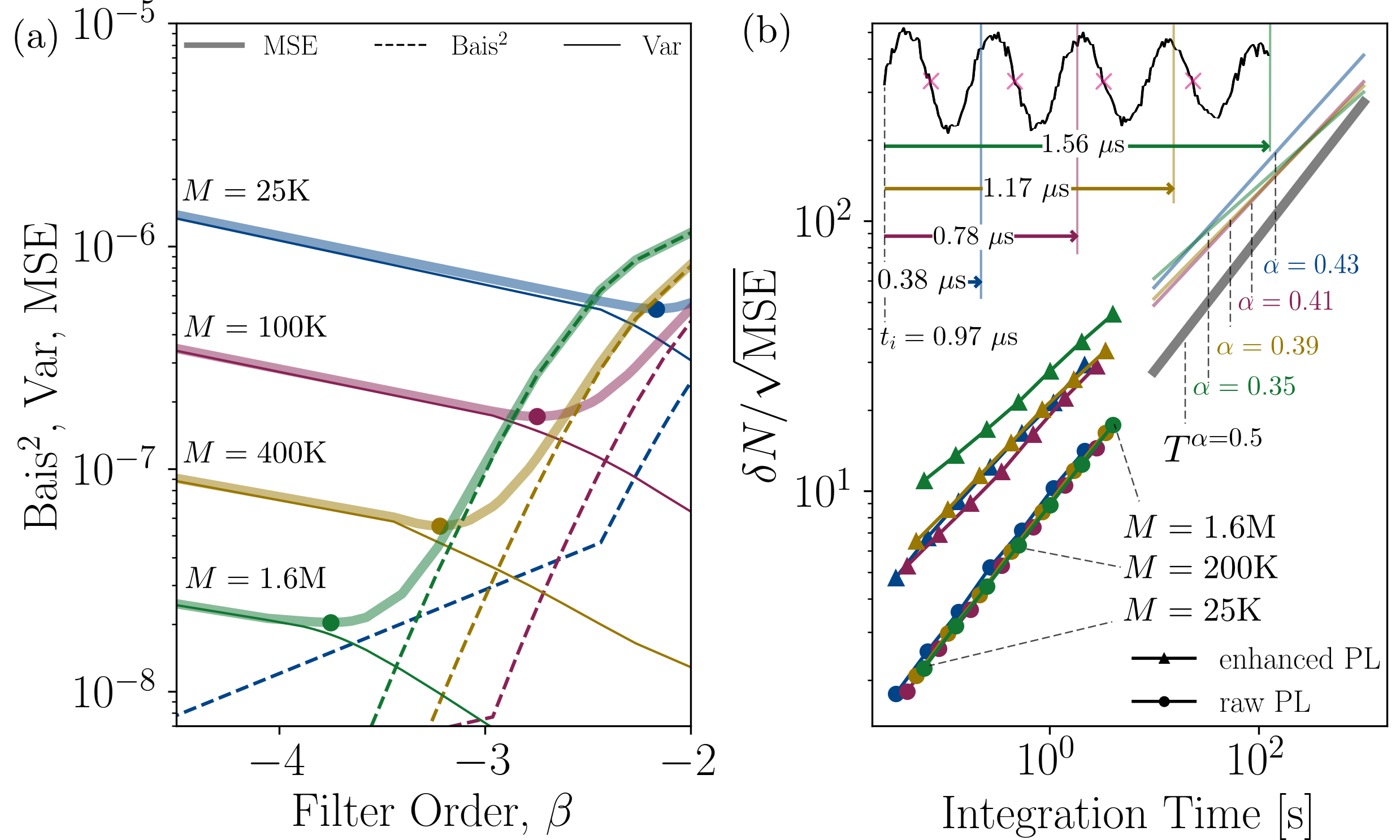
Figure 2: (a) Bias-variance trade-off with respect to filter order for PL taken between $[t_{i}=0.97~{}\mu$s, $t_{f}=2.14~{}\mu$s] at $f_{\text{sample}}\sim 128$ MHz including 3 $N_{\text{SD}}$ points. The MSE minima (i.e., optimum filter orders) are identified, with dots. (b) SNR with respect to total integration time with different PL durations. Dots represent the original PL SNR, and triangle markers represent TMT-enhanced PL data. Each marker at the same line stands for a specific $M$ number ranging from 25K to 1.6M with doubling $M$ numbers each time. Colors represent different PL durations, each starting from $t_{i}=0.97~{}\mu$s, to various $t_{f}$ values (blue, red, yellow, and green lines have $t_{f}$ values 1.36 $\mu$s, 1.75 $\mu$s, 2.14 $\mu$s, 2.53 $\mu$s, respectively). All PL time series are collected at $f_{\text{sample}}\sim 128~{}$MHz. All data points in (b) are generated at the corresponding optimum filter order.

IV Parameter settings and performance metrics

We use PL signals with readout contrast, $C=0.2143$, and with the average number of photons observed per repetition $n_{\text{ave}}=0.196$, which are experimentally realizable [59]. Since the number of photons collected per measurement is very low and hence uncorrelated, we assume that the photon statistics can be obtained from the Possionian distribution [16]. $M$ designates the number of repeated measurements to obtain each single data point over the PL signal. We assume that a PL signal is collected over some finite time duration $T_{I}=t_{f}-t_{i}$ so that the total number of data points is given by $T_{I}f_{\text{sample}}$. Furthermore, we use as the integration time $Mt_{f}$, which corresponds to the total time to collect the last data point of a PL signal.

A common metric to quantify the performance of an estimator, such as the TMT enhancement of PL is the mean squared error (MSE). For its assessment we perform an extra round of $N_{\text{exp}}$ independent experiments as,

$$\text{MSE}[N_{\text{sense}}^{\beta,q}]=\dfrac{1}{N_{\text{exp}}}\sum_{i=1}^{N_{\text{exp}}}[N_{\text{sense},i}^{\beta,q}-N^{*,q}]^{2},$$ (17)

where $\text{MSE}[N_{\text{sense}}^{\beta,q}]$ represents the MSE of TMT enhanced PL, $N^{*,q}$ is the true value for the number of photons and the superscript $q$ refers to $q^{\textit{th}}$ detection point of the accumulated PL in which the statistics are collected only for the detection regions. There are $N_{\text{SD}}$ such detection points all selected close to the negative slopes of the PL fringes, as marked by red crosses in the inset of Fig 2 (b). The MSE in Eq. (17) can be decomposed in terms of bias and variance as,

$$\text{MSE}[N_{\text{sense}}^{\beta,q}]=\text{Bias}[N_{\text{sense}}^{\beta,q}]^{2}+\text{Var}[N_{\text{sense}}^{\beta,q}],$$ (18)

where,

$$\text{Bias}[N_{\text{sense}}^{\beta,q}] =\sum_{i}[N_{\text{sense},i}^{\beta,q}-N^{*,q}]/N_{\text{exp}},$$ (19)

$$\text{Var}[N_{\text{sense}}^{\beta,q}] =\sum_{i}[N_{\text{sense},i}^{\beta,q}-\overline{N_{\text{sense},i}^{\beta,q}}]^{2}/N_{\text{exp}},$$ (20)

where the overline represents the sample mean. For our results, we use $N_{\text{exp}}=2000$, and consider PLs with various $N_{\text{SD}}$ numbers ranging from one to nine. To facilitate comparing PL streams of varying durations, we introduce fringe-averaged MSE values as, $\text{MSE}[N_{\text{sense}}^{\beta}]=\sum_{q=1}^{N_{\text{SD}}}\text{MSE}[N_{\text{sense}}^{\beta,q}]/N_{\text{SD}}$.

V Results and discussion

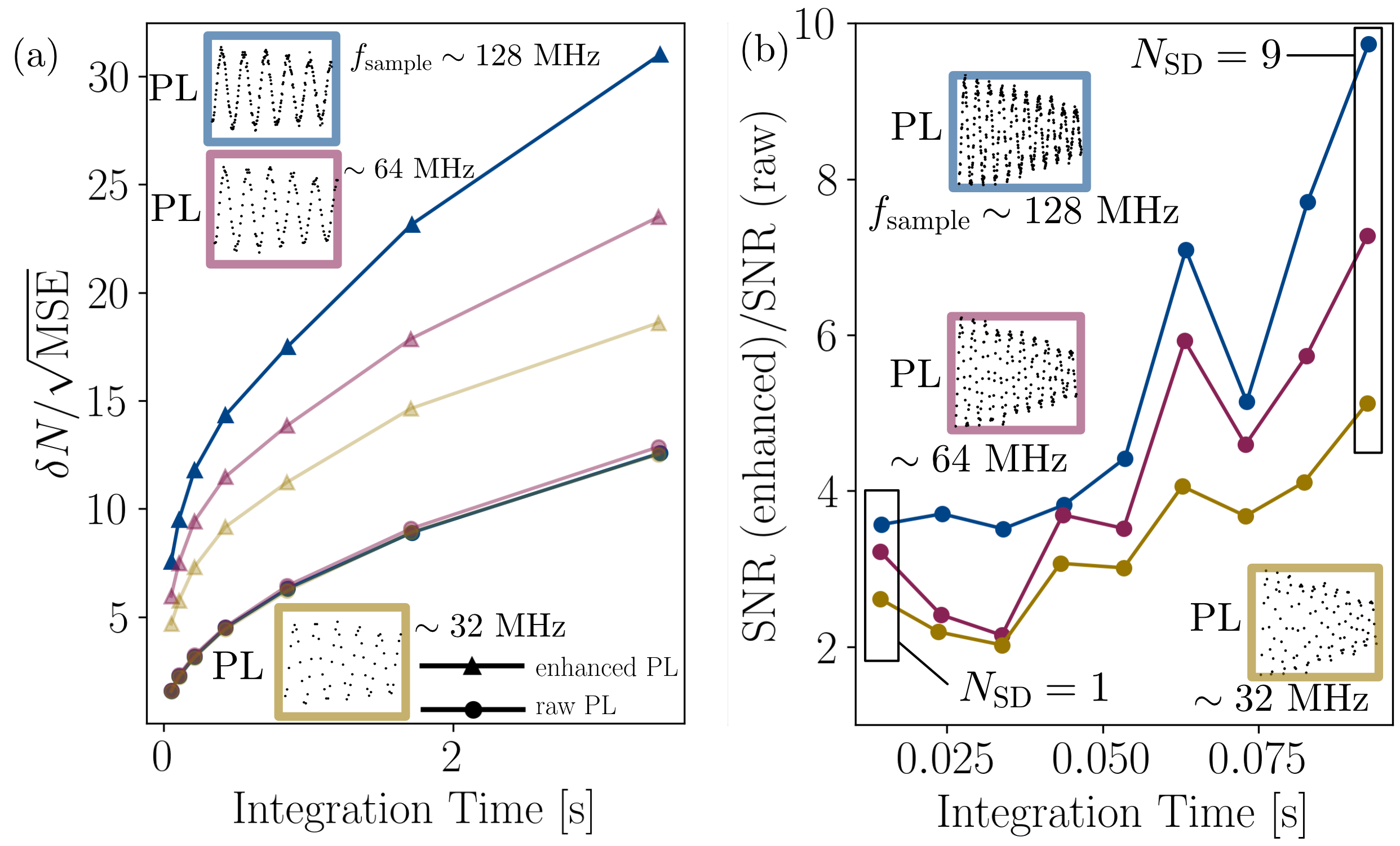
Figure 3: (a) SNR with respect to total integration time for PL acquired at various $f_{\text{sample}}$ values with fixed PL durations collected in the time interval $T_{I}=1.93~{}\mu$s ($[t_{i}=0.2~{}\mu$s, $t_{f}=2.13~{}\mu$s]) including 5 $N_{\text{SD}}$ points. Yellow, red, and blue lines represent the PL data with sampling frequencies approximately $32$ MHz, $64$ MHz, and $128$ MHz, respectively, as indicated by the insets. Lines with circle markers represent raw PL, and those with triangle markers indicate TMT-enhanced data obtained with optimum filter order. (b) Each subplot displays the performance gain from the TMT method for different PL durations at fixed $M=25$ K. The leftmost data point represents the gain of PL with duration corresponding to one detection point, and the rightmost data point is the longest PL which includes 9 $N_{\text{SD}}$ points in total. Each data point from left to right along the horizontal axis indicates one increment in the $N_{\text{SD}}$ number. For each subplot longest PL was collected between the time interval $[t_{i}=0.2~{}\mu$s, $t_{f}=3.7~{}\mu$s]. The subplots from top to bottom represent the PL data with sampling frequencies approximately $32$ MHz, $64$ MHz, and $128$ MHz, respectively, as indicated by the insets. All of the TMT enhanced data obtained with the filter order that minimizes the MSE of the calibration PL.

To put it into context, first, we would like to delineate the bias-variance trade-off by examining two extreme limits of the wavelet filter order, $\beta$. As the lower extreme $\beta\rightarrow-\infty$ corresponds to the raw PL limit (i.e., without wavelet denoising) where $N_{\text{sense}}^{\beta}$ approaches to $N_{\text{sense}}$. This regime governs low-bias/high-variance statistics for the random variable $N_{\text{sense}}^{\beta}$. The other extreme limit $\beta\rightarrow\infty$ ($N_{\text{sense}}\rightarrow\mathcal{K}$) imposes high-bias/low-variance. Thus, there is a bias-variance trade-off that should be optimized for obtaining minimum MSE. In Fig. 2 (a), we plot this trade-off as a function of filter order for various PLs generated with different $M$ values. For low filter orders the squared bias is extremely small, while for high filter orders, MSE gets dominated by bias. The optimum order values, $\beta_{\text{opt}}$, (marked with dots in Fig. 2 (a)) minimize the MSE, and they get smaller for higher $M$.

In Fig. 2 (b) we display signal-to-noise ratio (SNR), defined as the signal amplitude due to the sensing field, $\delta N$, divided by the noise amplitude obtained as the square root of MSE with respect to the total integration time. The scaling of SNR with respect to the integration time can be expressed as $c(Mt_{f})^{\alpha}$, where we refer to $c$ as the prefactor and $\alpha$ as the exponent. The SNR lines constructed with different $M$ values for specific PL duration and fixed sampling frequency $f_{\text{sample}}$, possess different exponents, all of which are below that of SQL (i.e., $\alpha<0.5$). Fortunately, despite the inferior exponent, filtered-SNR lines are exalted by very large prefactors resulting in significant performance gain. These scaling traits are the ramifications of the shrinkage of margin-exceeding points by means of hard thresholding. While the pruning of data points to the closest margin value $(u_{j,k}$ or $l_{j,k})$ causes partial information loss, again the same pruning yields a large prefactor due to decreased variance and hence, reduced MSE overall. Because of its $\alpha<0.5$ exponent, TMT-enhanced PL favors low-time-budget sensing applications. Nevertheless, for all practical purposes, this embraces very large integration times as seen by the crossing of their asymptotic behaviors (around $\sim 350$ seconds for the green line).

In Fig. 3 (a), this time we show SNR of varying $f_{\text{sample}}$ for both enhanced and raw signal at fixed PL duration $T_{I}$. Along the same line, the data points represent doubly ascending $M$ numbers, from 25K to 1.6M. For the raw PL, as expected, changing the sampling frequency does not improve SNR as it is the $M$ value that sets the number of detection points. However, TMT-enhanced PLs show an improvement as $f_{\text{sample}}$ increased due to more accurate $\omega_{\text{temp}}$ prediction, thanks to the elevated number of data points over the same PL duration. We believe that this is an important property of the TMT filter which might become useful when sensing a large magnetic field in which PL needs to be sampled with high $f_{\text{sample}}$ to prevent phase wrapping.

In general, TMT becomes a minimum MSE estimator, when operated at $\beta_{\text{opt}}$. However, in daylight applications, determining the optimal value for $\beta$ requires the knowledge of the true value of the number of photons at each fringe, $N^{*,q}$, which is the parameter we would like to estimate in the first place. At this point, the calibration PL becomes handy so that the determination of filter order can be obtained from the calibration signal. Even though this value does not yield the optimum order for sensing PL, as long as order-dependent parameters ($T_{I},M,f_{\text{sample}}$) are the kept same, the optimum filter order for sensing protocol is expected to be close to the one in the calibration PL, especially in long PL durations in which the filter order, $\beta$, becomes more accurate. To substantiate this claim, in Fig.3 (b), we operate at the filter order that minimizes the MSE of the calibration PL (unlike the previous results). To directly assess its performance improvement, SNR of TMT-enhanced-PL is normalized to that of raw-PL, i.e., $\sqrt{\text{MSE}[N_{\text{sense}}^{\text{raw}}]/\text{MSE}[N_{\text{sense}}^{\beta}}]$, where $\text{MSE}[N_{\text{sense}}^{\text{raw}}]$ is the MSE of the PL before enhancement. Here, we also compare three different sampling regimes. Increasing the duration of PL at a fixed sampling rate and $M=25$K, in general, refines the performance as the template can be estimated $\mathcal{K}(t,\omega_{\text{temp}})$ more accurately so that, filter order employed, $\beta$, can be larger. Since we take average MSE over all possible slope detection points simultaneously, the addition of more slope detection points results in a non-monotonic performance profile.

Overall, with long PL acquisitions and with modest $M$ values, it is possible to reach a significant PL enhancement up to an order of magnitude for each slope detection point on average. In principle, there is no fundamental barrier to performance improvement via TMT, other than $T_{2}^{*}$ decay factor. The reason is that the dephasing of NV^- due to environmental coupling makes the kernel in Eq. (8) inefficient for PL durations after some $t_{f}$ value due to diminishing contrast between $n_{0}$ and $n_{1}$. In this respect, TMT-boosted performance would be even higher for the isotopically purified NV-center with $T_{2}^{*}$ reaching $90~{}\mu$s [60], or by combining with other measures like dynamical decoupling pulse sequences [16].

VI Conclusion

In summary, we present a wavelet-based PL denoising technique that can increase the SNR up to an order of magnitude with respect to SQL. This improvement’s functional dependence with respect to integration time is dominated by the large prefactor as opposed to the scaling exponent. Being applied as a post-processing over the PL data, TMT has practical simplicity and versatility. Our proof of principle computational assessment relied on a single NV center DC magnetometry. However, we also think that the method holds great promise for ensemble sensing and for various time-dependent fields.

Appendix

In this appendix, we intend to give some preliminary information about wavelets to bridge with the material in Sec. III.

VI.1 Continuous wavelet transform

The continuous wavelet transform of a square integrable signal, $x(t)$, can be written as,

$$D(a,b)=\dfrac{1}{\sqrt{a}}\int^{\infty}_{-\infty}x(t)\,\psi^{*}\left(\dfrac{t-b}{a}\right)dt,$$ (21)

where $a$ and $b$ denote the dilation and translation parameters of the wavelet function, and $*$ represents its complex conjugation. From a mathematical point of view, we convolve $x(t)$ with some $\psi(t)$ which is localized both in the time and frequency domain, instead of sinusoidal functions that have frequency localization only as in Fourier transform. This enables time-frequency localization of the $x(t)$ simultaneously. It is important to note that, the complete representation of $x(t)$ requires the knowledge of $D(a,b)$ for each infinitely small step of $a$ and $b$ which constitutes a highly redundant representation of the signal.

VI.2 Continuous time discrete wavelet transform

It is possible to provide a more compact representation of the original signal by discretizing the scale and translation parameters of the wavelet function as,

$$\psi_{j,k}=\psi\left(\dfrac{t-kb_{0}a_{0}^{j}}{a_{0}^{j}}\right)/\sqrt{a_{0}^{j}}\,,$$ (22)

where $j,k\in Z$. If we consider a dyadically-grided scale and translation parameters ($a_{0}=2$ and $b_{0}=1$, as an example) provided that, $\psi_{j,k}$ constitutes a sufficiently tight frame [44], the function $x(t)$ can be expressed in linear combinations of wavelets at different scales ($j$) and locations ($k$),

$$x(t)=\sum_{j}\sum_{k}d_{j,k}\psi_{j,k}.$$ (23)

where $d_{j,k}=\langle x(t),\psi_{j,k}(t)\rangle=\int_{-\infty}^{\infty}x(t)\psi_{j,k}(t)dt$. For $x(t)$ with non-vanishing mean the summation over $j$ requires infinitely many terms, since, $\int\psi_{j,k}(t)dt=0$. This can be visualized in the frequency domain as indicated in Fig. 1 (b), increasing $j$ by one unit, just halves the bandwidth of the wavelet which has no zero-frequency component for any finite value of $j$. To overcome this difficulty, another set of functions, called as scaling functions $\phi_{j,k}$, can be introduced with non-zero mean. Scaling functions are orthogonal to wavelets at the same scale, yet they form a basis for the wavelets at the lower scale, for instance, so-called, the mother wavelet can be expressed as [56],

$$\psi_{0,0}(t)=\sum_{k}h_{1}(k)\sqrt{2}\phi_{0,0}(2t-k),$$ (24)

where $h_{1}(k)$ is some coefficient depending on the wavelet type, and $\phi=\phi_{0,0}$ is termed as the father wavelet as an analog to the mother wavelet. Father wavelet can be utilized to create scaling functions at different scales and location as $\phi_{j,k}=2^{-j/2}\phi(2^{-j}t-k)$. Then, function $x(t)$ can be expressed more conveniently at given scale $j_{0}$ as,

$$x(t)=\sum_{k=-\infty}^{\infty}c_{j_{0},k}\phi_{j_{0},k}(t)+\sum_{j=-\infty}^{j_{0}}\sum_{k=-\infty}^{\infty}d_{j,k}\psi_{j,k}(t),$$ (25)

$c_{j,k}=\langle x(t),\phi_{j,k}(t)\rangle$ and $d_{j,k}$ are called as approximation and detail coefficients, respectively.

VI.3 Discrete time fast wavelet transform and undecimated wavelet transform

For discrete time signal, the DWT can be calculated by half-band-lowpass and half-band-highpass filters. Since the lower or higher half of the frequencies are removed for the signal of interest the output discrete-time signals can be decimated by two without loss of information according to Nyquist sampling theorem, so that,

$$c_{j,k} =\sum_{m}h_{0}(m-2k)c_{j-1,m},$$ (26)

$$d_{j,k} =\sum_{m}h_{1}(m-2k)c_{j-1,m},$$ (27)

where, $c_{j,k}$ and $d_{j,k}$ are approximation and detail coefficients at the $j$th detail level, respectively. $h_{0}$ ($h_{1}$) is half-band-lowpass (half-band-bandpass) filters and the index $2k$ implements the decimation provided that the filters $h_{0}$ and $h_{1}$ satisfy the properties of quadrature mirror filters and they are the coefficients connecting the wavelet and scaling functions at different scale as Eq. (24) and,

$$\phi_{0,0}(t)=\sum_{k}h_{0}(k)\sqrt{2}\phi_{0,0}(2t-k).$$ (28)

References

- Wolfowicz et al. [2021] G. Wolfowicz, F. J. Heremans, C. P. Anderson, S. Kanai, H. Seo, A. Gali, G. Galli, and D. D. Awschalom, Quantum guidelines for solid-state spin defects, Nature Reviews Materials 6, 906 (2021).
- Manson et al. [2018] N. B. Manson, M. Hedges, M. S. J. Barson, R. Ahlefeldt, M. W. Doherty, H. Abe, T. Ohshima, and M. J. Sellars, Nv–n+ pair centre in 1b diamond, New Journal of Physics 20, 113037 (2018).
- Abobeih et al. [2018] M. H. Abobeih, J. Cramer, M. A. Bakker, N. Kalb, M. Markham, D. J. Twitchen, and T. H. Taminiau, One-second coherence for a single electron spin coupled to a multi-qubit nuclear-spin environment, Nature Communications 9, 2552 (2018).
- Degen [2008] C. L. Degen, Scanning magnetic field microscope with a diamond single-spin sensor, Applied Physics Letters 92, 243111 (2008), https://pubs.aip.org/aip/apl/article-pdf/doi/10.1063/1.2943282/14395578/243111_1_online.pdf .
- Taylor et al. [2008] J. M. Taylor, P. Cappellaro, L. Childress, L. Jiang, D. Budker, P. R. Hemmer, A. Yacoby, R. Walsworth, and M. D. Lukin, High-sensitivity diamond magnetometer with nanoscale resolution, Nature Physics 4, 810 (2008).
- Dolde et al. [2011] F. Dolde, H. Fedder, M. W. Doherty, T. Nöbauer, F. Rempp, G. Balasubramanian, T. Wolf, F. Reinhard, L. C. L. Hollenberg, F. Jelezko, and J. Wrachtrup, Electric-field sensing using single diamond spins, Nature Physics 7, 459 (2011).
- Casola et al. [2018] F. Casola, T. van der Sar, and A. Yacoby, Probing condensed matter physics with magnetometry based on nitrogen-vacancy centres in diamond, Nature Reviews Materials 3, 17088 (2018).
- Barson et al. [2017] M. S. J. Barson, P. Peddibhotla, P. Ovartchaiyapong, K. Ganesan, R. L. Taylor, M. Gebert, Z. Mielens, B. Koslowski, D. A. Simpson, L. P. McGuinness, J. McCallum, S. Prawer, S. Onoda, T. Ohshima, A. C. Bleszynski Jayich, F. Jelezko, N. B. Manson, and M. W. Doherty, Nanomechanical sensing using spins in diamond, Nano Letters 17, 1496 (2017).
- Kucsko et al. [2013] G. Kucsko, P. C. Maurer, N. Y. Yao, M. Kubo, H. J. Noh, P. K. Lo, H. Park, and M. D. Lukin, Nanometre-scale thermometry in a living cell, Nature 500, 54 (2013).
- Neumann et al. [2013] P. Neumann, I. Jakobi, F. Dolde, C. Burk, R. Reuter, G. Waldherr, J. Honert, T. Wolf, A. Brunner, J. H. Shim, D. Suter, H. Sumiya, J. Isoya, and J. Wrachtrup, High-precision nanoscale temperature sensing using single defects in diamond, Nano Letters 13, 2738 (2013).
- Ledbetter et al. [2012] M. P. Ledbetter, K. Jensen, R. Fischer, A. Jarmola, and D. Budker, Gyroscopes based on nitrogen-vacancy centers in diamond, Phys. Rev. A 86, 052116 (2012).
- Li et al. [2022] C. Li, R. Soleyman, M. Kohandel, and P. Cappellaro, Sars-cov-2 quantum sensor based on nitrogen-vacancy centers in diamond, Nano Letters 22, 43 (2022).
- Aslam et al. [2023] N. Aslam, H. Zhou, E. K. Urbach, M. J. Turner, R. L. Walsworth, M. D. Lukin, and H. Park, Quantum sensors for biomedical applications, Nature Reviews Physics 5, 157 (2023).
- Abobeih et al. [2019] M. H. Abobeih, J. Randall, C. E. Bradley, H. P. Bartling, M. A. Bakker, M. J. Degen, M. Markham, D. J. Twitchen, and T. H. Taminiau, Atomic-scale imaging of a 27-nuclear-spin cluster using a quantum sensor, Nature 576, 411 (2019).
- van de Stolpe et al. [2023] G. L. van de Stolpe, D. P. Kwiatkowski, C. E. Bradley, J. Randall, S. A. Breitweiser, L. C. Bassett, M. Markham, D. J. Twitchen, and T. H. Taminiau, Mapping a 50-spin-qubit network through correlated sensing, (2023), arXiv:2307.06939 [quant-ph] .
- Barry et al. [2020] J. F. Barry, J. M. Schloss, E. Bauch, M. J. Turner, C. A. Hart, L. M. Pham, and R. L. Walsworth, Sensitivity optimization for nv-diamond magnetometry, Rev. Mod. Phys. 92, 015004 (2020).
- Zheng et al. [2022] W. Zheng, K. Bian, X. Chen, Y. Shen, S. Zhang, R. Stöhr, A. Denisenko, J. Wrachtrup, S. Yang, and Y. Jiang, Coherence enhancement of solid-state qubits by local manipulation of the electron spin bath, Nature Physics 18, 1317 (2022).
- Steiner et al. [2010] M. Steiner, P. Neumann, J. Beck, F. Jelezko, and J. Wrachtrup, Universal enhancement of the optical readout fidelity of single electron spins at nitrogen-vacancy centers in diamond, Phys. Rev. B 81, 035205 (2010).
- Le Sage et al. [2012] D. Le Sage, L. M. Pham, N. Bar-Gill, C. Belthangady, M. D. Lukin, A. Yacoby, and R. L. Walsworth, Efficient photon detection from color centers in a diamond optical waveguide, Phys. Rev. B 85, 121202 (2012).
- Hopper et al. [2018] D. A. Hopper, R. R. Grote, S. M. Parks, and L. C. Bassett, Amplified sensitivity of nitrogen-vacancy spins in nanodiamonds using all-optical charge readout, ACS Nano 12, 4678 (2018).
- Jaskula et al. [2019] J.-C. Jaskula, B. Shields, E. Bauch, M. Lukin, A. Trifonov, and R. Walsworth, Improved quantum sensing with a single solid-state spin via spin-to-charge conversion, Phys. Rev. Appl. 11, 064003 (2019).
- Orphal-Kobin et al. [2023] L. Orphal-Kobin, K. Unterguggenberger, T. Pregnolato, N. Kemf, M. Matalla, R.-S. Unger, I. Ostermay, G. Pieplow, and T. Schröder, Optically coherent nitrogen-vacancy defect centers in diamond nanostructures, Phys. Rev. X 13, 011042 (2023).
- Sahin et al. [2022] O. Sahin, E. de Leon Sanchez, S. Conti, A. Akkiraju, P. Reshetikhin, E. Druga, A. Aggarwal, B. Gilbert, S. Bhave, and A. Ajoy, High field magnetometry with hyperpolarized nuclear spins, Nature Communications 13, 5486 (2022).
- Mamin et al. [2014] H. J. Mamin, M. H. Sherwood, M. Kim, C. T. Rettner, K. Ohno, D. D. Awschalom, and D. Rugar, Multipulse double-quantum magnetometry with near-surface nitrogen-vacancy centers, Phys. Rev. Lett. 113, 030803 (2014).
- Jarmola et al. [2021] A. Jarmola, S. Lourette, V. M. Acosta, A. G. Birdwell, P. Blümler, D. Budker, T. Ivanov, and V. S. Malinovsky, Demonstration of diamond nuclear spin gyroscope, Science Advances 7, eabl3840 (2021), https://www.science.org/doi/pdf/10.1126/sciadv.abl3840 .
- Jiang et al. [2009] L. Jiang, J. S. Hodges, J. R. Maze, P. Maurer, J. M. Taylor, D. G. Cory, P. R. Hemmer, R. L. Walsworth, A. Yacoby, A. S. Zibrov, and M. D. Lukin, Repetitive readout of a single electronic spin via quantum logic with nuclear spin ancillae, Science 326, 267 (2009), https://www.science.org/doi/pdf/10.1126/science.1176496 .
- Neumann et al. [2010] P. Neumann, J. Beck, M. Steiner, F. Rempp, H. Fedder, P. R. Hemmer, J. Wrachtrup, and F. Jelezko, Single-shot readout of a single nuclear spin, Science 329, 542 (2010), https://www.science.org/doi/pdf/10.1126/science.1189075 .
- Lovchinsky et al. [2016] I. Lovchinsky, A. O. Sushkov, E. Urbach, N. P. de Leon, S. Choi, K. D. Greve, R. Evans, R. Gertner, E. Bersin, C. Müller, L. McGuinness, F. Jelezko, R. L. Walsworth, H. Park, and M. D. Lukin, Nuclear magnetic resonance detection and spectroscopy of single proteins using quantum logic, Science 351, 836 (2016), https://www.science.org/doi/pdf/10.1126/science.aad8022 .
- Zhao et al. [2011] N. Zhao, J.-L. Hu, S.-W. Ho, J. T. Wan, and R. Liu, Atomic-scale magnetometry of distant nuclear spin clusters via nitrogen-vacancy spin in diamond, Nature Nantech. 6, 242 (2011).
- Kwiatkowski et al. [2020] D. Kwiatkowski, P. Szańkowski, and L. Cywiński, Influence of nuclear spin polarization on the spin-echo signal of an nv-center qubit, Phys. Rev. B 101, 155412 (2020).
- Onizhuk and Galli [2023] M. Onizhuk and G. Galli, Bath-limited dynamics of nuclear spins in solid-state spin platforms, Phys. Rev. B 108, 075306 (2023).
- Rovny et al. [2022] J. Rovny, Z. Yuan, M. Fitzpatrick, A. I. Abdalla, L. Futamura, C. Fox, M. C. Cambria, S. Kolkowitz, and N. P. de Leon, Nanoscale covariance magnetometry with diamond quantum sensors, Science 378, 1301 (2022), https://www.science.org/doi/pdf/10.1126/science.ade9858 .
- Wang et al. [2023] P. Wang, W. Yang, and R. Liu, Using weak measurements to synthesize projective measurement of nonconserved observables of weakly coupled nuclear spins, Phys. Rev. Appl. 19, 054037 (2023).
- Nusran et al. [2012] N. M. Nusran, M. U. Momeen, and M. V. G. Dutt, High-dynamic-range magnetometry with a single electronic spin in diamond, Nature Nanotechnology 7, 109 (2012).
- Dinani et al. [2019] H. T. Dinani, D. W. Berry, R. Gonzalez, J. R. Maze, and C. Bonato, Bayesian estimation for quantum sensing in the absence of single-shot detection, Phys. Rev. B 99, 125413 (2019).
- Zohar et al. [2023] I. Zohar, B. Haylock, Y. Romach, M. J. Arshad, N. Halay, N. Drucker, R. Stöhr, A. Denisenko, Y. Cohen, C. Bonato, and A. Finkler, Real-time frequency estimation of a qubit without single-shot-readout, Quantum Science and Technology 8, 035017 (2023).
- Braun et al. [2018] D. Braun, G. Adesso, F. Benatti, R. Floreanini, U. Marzolino, M. W. Mitchell, and S. Pirandola, Quantum-enhanced measurements without entanglement, Rev. Mod. Phys. 90, 035006 (2018).
- Degen et al. [2017] C. L. Degen, F. Reinhard, and P. Cappellaro, Quantum sensing, Rev. Mod. Phys. 89, 035002 (2017).
- Braun and Popescu [2014] D. Braun and S. Popescu, Coherently enhanced measurements in classical mechanics, Quantum Meas. Quantum Metrol. 2, 44 (2014).
- [40] J. M. E. Fraisse and D. Braun, Coherent averaging, Ann. Phys. 527, 701, https://onlinelibrary.wiley.com/doi/pdf/10.1002/andp.201500169 .
- Xie et al. [2023] T. Xie, Z. Zhao, S. Xu, X. Kong, Z. Yang, M. Wang, Y. Wang, F. Shi, and J. Du, 99.92-fidelity cnot gates in solids by noise filtering, Phys. Rev. Lett. 130, 030601 (2023).
- Xu et al. [2023] N. Xu, F. Zhou, X. Ye, X. Lin, B. Chen, T. Zhang, F. Yue, B. Chen, Y. Wang, and J. Du, Noise prediction and reduction of single electron spin by deep-learning-enhanced feedforward control, Nano Letters 23, 2460 (2023).
- Gupta et al. [2016] A. Gupta, L. Hacquebard, and L. Childress, Efficient signal processing for time-resolved fluorescence detection of nitrogen-vacancy spins in diamond, J. Opt. Soc. Am. B 33, B28 (2016).
- Daubechies [1992] I. Daubechies, Ten lectures on wavelets (SIAM, 1992).
- Xu et al. [2016] N. Xu, F. Jiang, Y. Tian, J. Ye, F. Shi, H. Lv, Y. Wang, J. Wrachtrup, and J. Du, Wavelet-based fast time-resolved magnetic sensing with electronic spins in diamond, Phys. Rev. B 93, 161117 (2016).
- Güldeste and Bulutay [2022] E. T. Güldeste and C. Bulutay, Wavelet resolved coherence beating in the overhauser field of a thermal nuclear spin ensemble, Phys. Rev. B 105, 075202 (2022).
- Seedhouse et al. [2023] A. E. Seedhouse, N. D. Stuyck, S. Serrano, T. Tanttu, W. Gilbert, J. Y. Huang, F. E. Hudson, K. M. Itoh, A. Laucht, W. H. Lim, et al., Spatio-temporal correlations of noise in mos spin qubits, arXiv preprint arXiv:2309.12542 (2023).
- Doherty et al. [2013] M. W. Doherty, N. B. Manson, P. Delaney, F. Jelezko, J. Wrachtrup, and L. C. Hollenberg, The nitrogen-vacancy colour centre in diamond, Physics Reports 528, 1 (2013), the nitrogen-vacancy colour centre in diamond.
- Jamonneau et al. [2016] P. Jamonneau, M. Lesik, J. P. Tetienne, I. Alvizu, L. Mayer, A. Dréau, S. Kosen, J.-F. Roch, S. Pezzagna, J. Meijer, T. Teraji, Y. Kubo, P. Bertet, J. R. Maze, and V. Jacques, Competition between electric field and magnetic field noise in the decoherence of a single spin in diamond, Phys. Rev. B 93, 024305 (2016).
- Maze et al. [2012] J. R. Maze, A. Dréau, V. Waselowski, H. Duarte, J.-F. Roch, and V. Jacques, Free induction decay of single spins in diamond, New Journal of Physics 14, 103041 (2012).
- Zhao et al. [2012] N. Zhao, S.-W. Ho, and R.-B. Liu, Decoherence and dynamical decoupling control of nitrogen vacancy center electron spins in nuclear spin baths, Phys. Rev. B 85, 115303 (2012).
- Güldeste and Bulutay [2018] E. T. Güldeste and C. Bulutay, Loschmidt echo driven by hyperfine and electric-quadrupole interactions in nanoscale nuclear spin baths, Phys. Rev. B 98, 085202 (2018).
- Yang et al. [2020] Z.-S. Yang, Y.-X. Wang, M.-J. Tao, W. Yang, M. Zhang, Q. Ai, and F.-G. Deng, Longitudinal relaxation of a nitrogen-vacancy center in a spin bath by generalized cluster-correlation expansion method, Annals of Physics 413, 168063 (2020).
- Onizhuk et al. [2021] M. Onizhuk, K. C. Miao, J. P. Blanton, H. Ma, C. P. Anderson, A. Bourassa, D. D. Awschalom, and G. Galli, Probing the coherence of solid-state qubits at avoided crossings, PRX Quantum 2, 010311 (2021).
- Mallat [1989] S. Mallat, A theory for multiresolution signal decomposition: the wavelet representation, IEEE Transactions on Pattern Analysis and Machine Intelligence 11, 674 (1989).
- Walker [2008] J. S. Walker, A primer on wavelets and their scientific applications (CRC press, 2008).
- Nason [2008] G. P. Nason, ed., Wavelet shrinkage, in Wavelet Methods in Statistics with R (Springer New York, New York, NY, 2008) pp. 83–132.
- Stéphane [2009] M. Stéphane, Chapter 7 - wavelet bases, in A Wavelet Tour of Signal Processing (Third Edition), edited by M. Stéphane (Academic Press, Boston, 2009) third edition ed., pp. 263–376.
- Shields et al. [2015] B. J. Shields, Q. P. Unterreithmeier, N. P. de Leon, H. Park, and M. D. Lukin, Efficient readout of a single spin state in diamond via spin-to-charge conversion, Phys. Rev. Lett. 114, 136402 (2015).
- Ishikawa et al. [2012] T. Ishikawa, K.-M. C. Fu, C. Santori, V. M. Acosta, R. G. Beausoleil, H. Watanabe, S. Shikata, and K. M. Itoh, Optical and spin coherence properties of nitrogen-vacancy centers placed in a 100 nm thick isotopically purified diamond layer, Nano Letters 12, 2083 (2012).