theoremTheorem

Playing in the Dark: No-regret Learning with Adversarial Constraints

1 Abstract

We study a generalization of the classic Online Convex Optimization (OCO) framework by considering additional long-term adversarial constraints. Specifically, after an online policy decides its action on a round, in addition to a convex cost function, the adversary also reveals a set of $k$ convex constraints. The cost and the constraint functions could change arbitrarily with time, and no information about the future functions is assumed to be available. In this paper, we propose a meta-policy that simultaneously achieves a sublinear cumulative constraint violation and a sublinear regret. This is achieved via a black box reduction of the constrained problem to the standard OCO problem for a recursively constructed sequence of surrogate cost functions. We show that optimal performance bounds can be achieved by solving the surrogate problem using any adaptive OCO policy enjoying a standard data-dependent regret bound. A new Lyapunov-based proof technique is presented that reveals a connection between regret and certain sequential inequalities through a novel decomposition result. We conclude the paper by highlighting applications to online multi-task learning and network control problems.

2 Introduction

Online Convex Optimization (OCO) is a standard framework for modelling and analyzing a broad class of online decision problems under uncertainty. In this problem, an online policy selects a sequence of actions from a convex feasible set over multiple rounds. After the policy selects an action on a round, the adversary reveals a convex cost function. The goal of a no-regret policy is to choose an action sequence so that its cumulative cost is not much larger than that of any fixed feasible action chosen in hindsight. In this paper, we consider a generalization of the above standard OCO framework where, in addition to a cost function, the adversary also reveals a collection of constraints of the form $g_{t,i}(x)\leq 0,i\in[k]$ on each round $t$. The goal is to design an online policy to control both the regret and the cumulative violation penalty optimally. This begets a natural question - Is it possible to efficiently reduce the constrained problem to an unconstrained OCO problem while obtaining the optimal regret and cumulative violation bounds? In this paper, we answer this question affirmatively in a constructive fashion.

Variants of the above problem arise in many applications, including online portfolio optimization with risk constraints, online resource allocation (e.g., CPU, memory, bandwidth) in cloud computing with time-varying demands, pay-per-click online ad markets with budget constraints (Liakopoulos et al., 2019), online recommendation systems, dynamic pricing, revenue management, robotics and path planning problems, and multi-armed bandits with fairness constraints (Sinha, 2023). Constrained optimization problems with a huge set of constraints can also be conveniently formulated in this framework. The necessity for revealing the constraints sequentially may arise, e.g., in communication-constrained settings, where it might be infeasible to reveal all constraints which define the feasible set (e.g., combinatorial auctions). To further motivate the problem, we now introduce a convex optimization over a hidden constraint set, which we call the Hidden Set problem.

The Hidden Set Problem:

Let $\Omega$ be an admissible set of actions which is known to the policy. Let $\Omega^{*}$, called the feasible set, be a closed and convex subset of $\Omega$. Due to a large number of defining constraints, the feasible set $\Omega^{*}$ is too complex to communicate to the policy a priori. However, an efficient separation oracle for $\Omega^{*}$ is assumed to be available. On the $t$^th round, the policy first selects an admissible action $x_{t}\in\Omega$ and then, the adversary reveals a convex cost function $f_{t}$ and some convex constraint of the form $g_{t}(x)\leq 0,$ which contains the unknown feasible set $\Omega^{*}$. As an example, the constraints could come from the separation oracle that, if $x_{t}$ is infeasible, outputs a hyperplane separating the current action $x_{t}\in\Omega$ and the hidden feasible set $\Omega^{*}$. The objective of the policy is to perform as well as any action from the hidden feasible set $\Omega^{*}$ in terms of the regret and the cumulative constraint violation metrics.

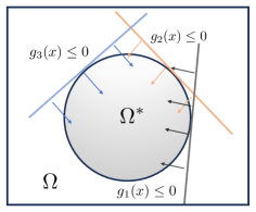
Figure 1: Illustrating the Hidden Set problem. In this figure, the sphere $\Omega^{*}$ is the hidden set. On every round $t$, the adversary reveals a hyperplane supporting $\Omega^{*}.$

2.1 Related Work

In a seminal paper, Zinkevich (2003) showed that the ubiquitous online gradient descent (OGD) policy achieves an $O(\sqrt{T})$ regret for convex cost functions with uniformly bounded sub-gradients. A number of follow-up papers proposed adaptive and parameter-free versions of OGD that do not need to know any non-causal information (Hazan et al., 2007; Orabona and Pál, 2018; Orabona, 2019). However, these lines of work do not consider additional constraints - a problem which has been systematically explored only recently (see Table 2 for a brief summary). The constraint functions could either be known a priori or revealed sequentially along with the cost functions.

Known and fixed constraints:

A number of papers considered the OCO problem with time-invariant constraints assumed to be known to the policy a priori (Yuan and Lamperski, 2018; Jenatton et al., 2016; Yu et al., 2017; Yu and Neely, 2016; Mahdavi et al., 2012). These papers relax the requirement that the online policy must satisfy the constraints exactly on each step. Instead, their main objective is to design an efficient policy which avoids the complicated projection step of the vanilla OGD policy while requiring that the cumulative constraint violations over the horizon grow sub-linearly. In this connection, Jenatton et al. (2016) and Yuan and Lamperski (2018) established a regret bound of $O(T^{\max(\beta,1-\beta)})$ and a cumulative constraint violation bound of $O(T^{1-\beta})$ for augmented Lagrangian-based primal-dual algorithms, where $0<\beta<1$ is a free parameter. For the same regret bound, Yi et al. (2021) improved the cumulative constraint violation bound to $O(T^{(1-\beta)/2})$, which was further improved to $O(1)$ by Guo et al. (2022) for the case $\beta=\nicefrac{{1}}{{2}}.$ In the case of fixed constraints and strongly convex losses, Guo et al. (2022) gave an algorithm which achieves $O(\log T)$ regret and $O(1)$ violation bounds while assuming access to the entire constraint functions and solving a convex problem on each round.

Adversarial and dynamic constraints:

Coming to the more challenging problem of time-varying constraint functions which we study in this paper, with the notable exceptions of neely2017online and georgios-cautious, most of the previous papers assume that the policy has access to some non-causal information, e.g., a uniform upper bound to the norm of the future gradients (jenatton2016adaptive; yu2017online; mahdavi2012trading; pmlr-v70-sun17a; yi2023distributed). This information is used by their proposed policies to construct an appropriate Lagrangian function or carefully select the step size schedule. liu2022simultaneously consider the problem of minimizing the dynamic regret by extending the virtual queue-based policy of (neely2017online). However, due to the dynamic benchmark, their regret bound explicitly depends on the temporal variation of the constraint functions. Recent work by yi2023distributed considers the case of convex constraint functions and convex or strongly convex cost functions in a distributed setting. In the case of convex cost functions, they establish an $O(T^{\max(\beta,1-\beta)})$ regret and an $O(T^{1-\beta/2})$ constraint violation bound for a primal-dual mirror descent policy without assuming Slater’s condition. However, their algorithm assumes a uniform upper bound to the norm of the gradients is known.

Drift-plus-penalty-based policies:

Closer to our work, neely2017online give a drift-plus-penalty-based policy that achieves an $O(\sqrt{T})$ regret and $O(\sqrt{T})$ cumulative violation penalty upon assuming Slater’s condition. In brief, Slater’s condition ensures the existence of a fixed feasible action $x^{*}$ such that all constraints hold strictly with a positive margin $\eta>0,$ i.e., $g_{t,i}(x^{*})<-\eta,\forall i,t$. Clearly, this condition precludes the important case of non-negative constraint functions (e.g., constraint functions of the form $\max(0,g_{t}(x))$). Furthermore, a sublinear violation bound obtained upon assuming Slater’s condition is loose by a quantity that increases linearly with the horizon-length $T$ compared to a sublinear violation bound obtained without this assumption. Worse, the regret bound presented in neely2017online diverges to infinity as $\eta\searrow 0.$ In a recent paper, yi2023distributed consider the same problem in a distributed setup and derive tighter bounds upon assuming Slater’s condition. georgios-cautious extend neely2017online’s result by considering a stronger comparator called the $S$-benchmark. The fixed action $x^{*}$ in an $S$-benchmark enjoys the property that the sum of the constraint functions evaluated at $x^{*}$ over any consecutive sequence of $S\geq 1$ rounds is non-positive. Without assuming Slater’s condition, they show that the drift-plus-penalty-based policy achieves a regret bound of $O(ST/V+\sqrt{T})$ and a violation penalty of $O(\sqrt{VT})$. Here, $V$ is an adjustable parameter that can take any value in $[S,T).$ Hence, a priori, their algorithm needs to know the value of the parameter $S,$ which, unfortunately, depends on the online constraints. Although these results are interesting, since the previous drift-plus-penalty-based algorithms are all based on linear approximations, none can be extended to prove improved bounds for the strongly convex case. In recent work, guo2022online consider the same problem for non-negative convex and strongly convex functions with convex constraints and obtain near-optimal performance bounds. However, their algorithm is inefficient as, instead of a single gradient-descent step per round (as in our and most of the previous algorithms), their algorithm solves a general convex optimization problem at every round. Moreover, their algorithm needs access to the full description of the constraint function $g_{t}(\cdot)$ for the optimization step, whereas ours and most of the previous algorithms need to know only the gradient and the value of the constraint function at the current action $x_{t}$. Lastly, their analysis is tailored for the hard constraints and, hence, their algorithm can not be extended to the more general $S$-benchmark, where it is necessary to compensate for constraint violations at some rounds with strictly satisfying constraints on some other rounds. Please refer to Table 2 for a brief summary of the results.

The Online Constraint Satisfaction (OCS) Problem:

We also study a special case of the above problem, called Online Constraint Satisfaction (OCS), that does not involve any cost function. In this problem, on every round $t$, $k$ constraints of the form $g_{t,i}(x)\leq 0$ are revealed to the policy in an online fashion, where the function $g_{t,i}$ comes from the $i$^th stream. The constraint functions could be unrestricted in sign - they may potentially take both positive and negative values within their admissible domain. The objective is to control the cumulative violation of each separate stream by choosing a common action sequence $\{x_{t}\}_{t\geq 1}$. To the best of our knowledge, the OCS problem has not been previously considered in the literature. Although the OCS problem can be reduced to the previous problem with dynamic constraints upon setting the cost function $f_{t}\equiv 0,\forall t$, this reduction turns out to be provably sub-optimal. In particular, without any assumption, the best-known bound for the cumulative violation for a single convex constraint is known to be $O(T^{3/4})$ and no violation penalty bound is known for strongly convex constraints (see Table 1). For the first time, we show that it is possible to achieve a cumulative violation bound of $O(\sqrt{ST})$ for convex constraints with the general $S$-benchmark and $O(\log T)$ for strongly convex constraints with the usual $1$-benchmark.

Reference	Constraints type	Benchmark	Violation	Algorithm	Assumption
jenatton2016adaptive	Fixed, convex	$1$	$O(T^{3/4})$	Primal-Dual GD	Known $G$
yuan2018online	Fixed, convex	$1$	$O(1)$	Primal-Dual MD	Fixed constraints
yu2017online	Stochastic, convex	$T$	$O(\sqrt{T})$	OGD+drift+penalty	Slater
yi2023distributed	Adversarial, convex	$1$	$O(\sqrt{T})$	Primal-Dual MD	Known $G$
pmlr-v70-sun17a	Adversarial, convex	$1$	$O(T^{3/4})$	OMD	Known $G$
neely2017online	Adversarial, convex	$1$	$O(\sqrt{T})$	OGD	Slater
georgios-cautious	Adversarial, convex, one constraint	$S$	$O(\sqrt{ST})$	OGD	Known $S$
guo2022online	Adversarial, convex	$1$	$O(T^{3/4})$	Convex opt. each round	Full access to $\{g_{t}\}_{t\geq 1}$
This paper	Adversarial, convex	$S$	$O(\sqrt{ST})$	Any adaptive	-
This paper	Adversarial, strongly-convex	$1$	$O(\log T)$	Any adaptive	-

Table 1: Summary of the results for the OCS problem. Results from other papers, which consider only the generalized OCO problem, have been appropriately adapted for the OCS problem by taking the cost function to be identically equal to zero and quoting the best violation bound. Excepting our paper, all other papers referenced above bound the cumulative violation over the entire horizon of length $T$, which is weaker than (4) for constraints assuming both positive and negative signs. $G$ is an upper bound to the norm of the gradients, $\alpha$ is the strong-convexity parameter; Abbreviations: MD= Mirror Descent, OMD = Online Mirror Descent, OGD = Online Gradient Descent.

2.2 Why are the above problems non-trivial?

Let us consider the OCS problem. A first attempt to solve the OCS problem could be to scalarize it by taking a fixed linear combination (e.g., the sum) of the constraint functions and then running a standard OCO policy on the scalarized cost functions. The above strategy immediately yields a sublinear regret guarantee on the same linear combination (i.e., the sum) of the constraint functions. However, since the constraint functions could take both positive and negative values, the constraint violation component of some streams could still be arbitrarily large even when the overall sum is small. Hence, this strategy does not yield individual cumulative violation bounds, where we need to control the more stringent $\ell_{\infty}$-norm of the cumulative violation vector. Hence, to meet the objective with this scalarization strategy, the “correct” linear combination of the constraints must be learned adaptively in an online fashion. This is exactly what our online meta-policy, which we propose in Section 4.3, does.

To get around the above issue, one may alternatively attempt to scalarize the OCS problem by considering a non-negative surrogate cost function, e.g., the hinge loss function, defined as $\hat{g}_{t,i}(x)=\max(0,g_{t,i}(x)),$ for each constraint $i\in[k]$. However, it can be easily seen that this transformation does not preserve the strong convexity as the function $\hat{g}_{t,i}$ is not strongly convex even when the original constraint function $g_{t,i}$ is strongly convex. Furthermore, the above strategy does not work even for convex functions for $S$-feasible benchmarks with $S\geq 2.$ This is because, due to the impossibility of cancellation of positive violations by strictly feasible constraints on different rounds, an $S$-feasible benchmark for the original constraints does not remain feasible for the transformed non-negative surrogate constraints (see Section 6). Finally, the above transformation fails in the case of stochastic constraints where the constraint is satisfied only in expectation, i.e., $\mathbb{E}g_{t}(x)\leq 0,\forall t\geq 1$ (yu2017online). The above discussion shows why designing an efficient and universal policy for the OCS problem, and consequently, for the generalized OCO problem - which generalizes OCS, is highly non-trivial.

2.3 Our contribution

In this paper, we consider two closely related online learning problems, namely (1) Online Constraint Satisfaction (OCS) and (2) Generalized OCO. In particular, we claim the following contributions.

1. We propose a general framework for designing efficient online learning policies for the Online Constraint Satisfaction (OCS) and the Generalized OCO problems with optimal regret and cumulative violation bounds. In contrast with the prior works, that establish performance bounds only for specific learning policies, we give a policy-agnostic black box reduction of the constrained problem to the standard OCO using any adaptive learning policy with a standard data-dependent regret bound. Consequently, efficient policies can be obtained by using known OCO sub-routines that exploit the special structure of the admissible action set (e.g., FTPL for combinatorial problems).

2. Our meta-policy for the OCS problem is parameter-free and does not need any non-causal information including, uniform upper bounds to the gradients or the strong-convexity parameters of the future constraint functions. Yet, the proposed policy achieves the optimal violation bounds without making any extraneous assumptions, such as Slater’s condition (see Table 1).

3. Tighter cumulative violation bounds for the Generalized OCO problem are obtained by using a new criterion - the non-negativity of the worst-case regret on a round (see Table 2). This replaces the stronger and often infeasible assumption on Slater’s condition in the literature. Surprisingly, it leads to an $O(\log T)$ violation bound for convex constraints and strongly convex cost functions.

4. As a by-product of our algorithm for the OCS problem, we obtain a new class of stabilizing control policies for the classic input-queued switching problem with adversarial arrival and service processes (see Section 7).

5. These results are established by introducing a new potential-based technique for simultaneously bounding the regret and constraint violation penalty. In brief, all performance guarantees in this paper are obtained by solving a recursive inequality which arises from plugging in off-the-shelf regret bounds in a new regret decomposition result. To the best of our knowledge, this is the first such separability result for this problem and might be of independent interest.

6. Thanks to the regret decomposition result, our proof arguments are compact requiring only a few lines of elementary algebra. This should be contrasted with long and intricate arguments in many of the papers cited above.

Summary of the results for the Generalized OCO problem Reference Constraints type Regret Violation Algorithm Assumption jenatton2016adaptive Fixed $O(T^{\max(\beta,1-\beta)})$ $O(T^{1-\beta/2})$ Primal-Dual GD Fixed constraints yuan2018online Fixed $O(T^{\max(\beta,1-\beta)})$ $O(T^{1-\beta/2})$ Primal-Dual MD Fixed constraints yi2021regret Fixed, convex $O(T^{\max(\beta,1-\beta)})$ $O(T^{(1-\beta)/2})$ OGD+drift+penalty Fixed constraints yi2023distributed Adversarial $O(T^{\max(\beta,1-\beta)})$ $O(T^{1-\beta/2})$ Primal-Dual MD Known $G$ yi2023distributed Adversarial, str-convex cost $O(\log(T))$ $O(\sqrt{T\log T})$ Primal-Dual MD Known $G,\alpha$ pmlr-v70-sun17a Adversarial $O(\sqrt{T})$ $O(T^{3/4})$ OMD Known $G$ neely2017online Adversarial $O(\sqrt{T})$ $O(\sqrt{T})$ OGD+drift+penalty Slater condition guo2022online Adversarial $O(\sqrt{T})$ $O(T^{3/4})$ Convex opt. each round Full access to $\{g_{t}\}$ guo2022online Adversarial, str-convex cost $O(\log T)$ $O(\sqrt{T\log T})$ Convex opt. each round Full access to $\{g_{t}\}$ This paper Adversarial $O(\sqrt{T})$ $O(T^{3/4})$ Any adaptive - This paper Adversarial $O(\sqrt{T})$ $O(\sqrt{T})$ Any adaptive $\textrm{Regret}_{T}\geq 0$ This paper Adversarial, str-convex cost $O(\log T)$ $O(\sqrt{T\log T})$ Any adaptive - This paper Adversarial, str-convex cost $O(\log T)$ $O(\frac{\log T}{\alpha})$ Any adaptive $\textrm{Regret}_{T}\geq 0$

Table 2: Summary of the results for the Generalized OCO problem. Unless mentioned otherwise, we assume $1$-feasibility, general convex constraints, and convex cost functions while stating the bounds. In the above, $0\leq\beta\leq 1$ is an adjustable parameter. The parameter $\alpha$ denotes the strong convexity parameter of the cost functions. $G$ denotes a uniform upper bound to the gradient of cost and constraint functions. $\textrm{Regret}_{T}$ denotes the worst-case regret against all static admissible actions.

On the methodological contribution:

Lyapunov or the potential function method has been extensively used in the literature for designing and analyzing control policies for linear and non-linear systems. The stochastic variant of the Lyapunov method, and especially the Foster-Lyapuov theorem, has played a pivotal role in designing stabilizing control policies for stochastic queueing networks (meyn2008control; neely2010stochastic). However, to the best of our knowledge, the application of these analytical tools to systems with adversarial dynamics has been quite limited in the literature. In this paper, we show how the Lyapunov and the drift-plus-penalty method neely2010stochastic can be seamlessly combined with the OCO framework to design new algorithms with tight performance bounds. We expect that the analytical methods developed in this paper can be generalized to more complex problems with adversarial inputs.

Note:

If a convex function $f$ is not differentiable at the point $x$ then by $\nabla f(x)$ we denote any sub-gradient of the function at $x$. Recall that any convex function could be non-differentiable only on a set of measure at most zero (convex_rockafeller72, Theorem 25.5). Hence, by smoothly perturbing at all points of non-differentiability by an infinitesimal amount, we can alternatively and without any loss of generality assume all cost and constraint functions to be differentiable without altering the regret/constraint violation bounds presented in this paper (hazan2007adaptive).

3 Preliminaries on Online Convex Optimization (OCO)

The standard online convex optimization problem can be viewed as a repeated game between an online policy and an adversary (hazan2016introduction). Let $\Omega\subseteq\mathbb{R}^{d}$ be a convex set, which we call the admissible set. On every round $t\geq 1,$ an online policy selects an action $x_{t}$ from the admissible set $\Omega.$ Upon seeing the currently selected action $x_{t}$, the adversary reveals a convex cost function $f_{t}:\Omega\mapsto\mathbb{R}$. The goal of the online policy is to choose an admissible action sequence $\{x_{t}\}_{t\geq 1}$ so that its total cost over any horizon of length $T$ is not much larger than the total cost incurred by any fixed admissible action $x^{*}\in\Omega$. More precisely, the objective of the policy is to minimize the static regret $\mathcal{R}_{T}$:

$$\mathcal{R}_{T}\equiv\sup_{x^{*}\in\Omega}\mathcal{R}_{T}(x^{*}),~{}\textrm{where~{}}\mathcal{R}_{T}(x^{*})\equiv\sum_{t=1}^{T}f_{t}(x_{t})-\sum_{t=1}^{T}f_{t}(x^{*}).$$ (1)

Algorithm 1 Online Gradient Descent (OGD)

0:  Non-empty closed convex set $\Omega\subseteq\mathbb{R}^{d}$, Sequence of convex cost functions $\{f_{t}\}_{t\geq 1},$ step sizes $\eta_{1},\eta_{2},\ldots,\eta_{T}>0.$

1:  Initialize $x_{1}$ arbitrarily

2:  for each round $t\geq 1$ do

3:     Predict $x_{t}$, observe $f_{t}$, incur a cost of $f_{t}(x_{t})$.

4:     Compute a (sub)-gradient $\nabla_{t}$ of $f_{t}$ at $x_{t}$. Let $G_{t}=||\nabla_{t}||_{2}.$

5:     Update $x_{t+1}=\Pi_{\Omega}(x_{t}-\eta_{t}\nabla_{t}).$

6:  end for

In a seminal paper, zinkevich2003online showed that the online gradient descent policy, given in Algorithm 1, with an appropriately chosen constant step size schedule, achieves a sublinear regret bound $\mathcal{R}_{T}=O(\sqrt{T})$ for convex cost functions with bounded (sub)-gradients. In this paper, we are interested in stronger adaptive regret bounds where the bound is given in terms of the norm of the gradients and the strong-convexity parameters of the online cost functions. In Theorem 1, we quote two standard results on such data-dependent adaptive regret bounds achieved by the standard OGD policy with appropriately chosen adaptive step size schedules.

Theorem 1.

Consider the generic OGD policy given in Algorithm 1.

1. (orabona2019modern, Theorem 4.14) Let the cost functions $\{f_{t}\}_{t\geq 1}$ be convex and the step size sequence be chosen as $\eta_{t}=\frac{\sqrt{2}D}{2\sqrt{\sum_{\tau=1}^{t-1}G_{\tau}^{2}}},t\geq 1,$ where $D$ is the diameter of the admissible set $\Omega$ and $G_{t}=\nabla f_{t}(x_{t}),t\geq 1.$ Then the OGD algorithm achieves the following regret bound:

   $$\mathcal{R}_{T}\leq\sqrt{2}D\sqrt{\sum_{t=1}^{T}G_{t}^{2}}.$$ (2)

2. (hazan2007adaptive, Theorem 2.1) Let the cost functions $\{f_{t}\}_{t\geq 1}$ be strongly convex and let $H_{t}>0$ be the strong-convexity parameter for the cost function $f_{t}$. Let the step size sequence be chosen as $\eta_{t}=\frac{1}{\sum_{s=1}^{t-1}H_{s}},t\geq 1.$ Then the OGD algorithm achieves the following regret bound:

   $$\mathcal{R}_{T}\leq\frac{1}{2}\sum_{t=1}^{T}\frac{G_{t}^{2}}{\sum_{s=1}^{t}H_{s}}.$$ (3)

Note that the above adaptive bounds are mentioned for the simplicity of the regret expressions and the corresponding policy and for no other particular reason. Similar regret bounds are known for a host of other online learning policies as well. For structured domains, one can use other algorithms such as AdaFTRL (orabona2018scale) which gives better regret bounds for high-dimensional problems. Furthermore, for problems with combinatorial structures, adaptive oracle-efficient algorithms, e.g., Follow-the-Perturbed-Leader (FTPL)-based policies, may be used (abernethy2014online, Theorem 11) (see Section 7). Our proposed meta-policy is oblivious to the particular online learning sub-routine being used to solve the surrogate OCO problem - all that is expected from the sub-routine are adaptive regret bounds comparable to (2) and (3). This property can be exploited to immediately extend the scope of our proposed algorithm to various other non-standard settings, e.g., delayed feedback (joulani2016delay).

4 The Online Constraint Satisfaction (OCS) Problem

We begin our discourse with the Online Constraint Satisfaction (OCS) problem, which does not contain any cost function. In this problem, the online learner is presented with an ordered $k$-tuple of convex constraints on each round. At each round, the constraints could be adversarially chosen, which are then revealed to the learner after it selects its action for that round. The objective is to choose actions sequentially so that the cumulative constraint violations corresponding to each component of the $k$-tuple grow sub-linearly with the horizon length. Although the OCS problem can be seen to be a special case of the generalized OCO problem, it is important as a standalone problem as well. In the following, we show that the online multi-task learning problem can be formulated as an instance of the OCS problem.

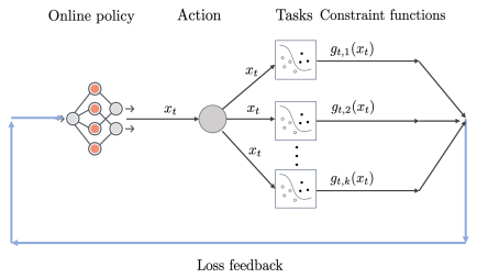
Figure 2: A schematic for the online multi-task learning problem

Example: Online Multi-task Learning:

Consider the problem of online multi-task learning where we train a single model to solve a number of related tasks (ruder2017overview; dekel2006online; murugesan2016adaptive). See Figure 2 for a simplified schematic. In this problem, the action $x_{t}$ naturally translates to the shared weight vector that encodes the model common to all tasks. The loss function for the $j$^th task on round $t$ is given by the function $g_{t,j}(\cdot),j\in[k].$ A task is assumed to be satisfactorily completed (e.g., correct prediction in the case of classification problems) on any round if the corresponding loss is non-positive. The objective of the multi-task learning problem is to sequentially predict the shared weight vectors $\{x_{t}\}_{t=1}^{T}$ so that the maximum cumulative loss of each task over any sub-interval grows sub-linearly with the length of the interval. Since the weight vector is shared across the tasks, the above goal would be impossible to achieve had the tasks not been related to each other (ruder2017overview). Hence, we make the assumption that there exists a fixed admissible action $x^{*}$ which could perform all the tasks satisfactorily. See Section 7 for an application of the tools and techniques developed for the OCS problem to a queueing problem.

4.1 Problem formulation

We now formalize the online constraint satisfaction (OCS) problem described above. Assume that on every round $t\geq 1$, an online policy selects an action $x_{t}$ from an admissible set $\Omega\subseteq\mathbb{R}^{d}$. After observing the current action $x_{t}$, an adversary outputs $k$ ordered constraints of the form $g_{t,i}(x)\leq 0$ where each $g_{t,i}:\Omega\mapsto\mathbb{R}$ is a convex function. As an example, in the problem of multi-task learning, each of the $k$ constraint sequences can be thought to belong to a specific task. The constraint functions are accessible to the policy via a first-order oracle, which returns only the values and the gradients (sub-gradients in the case of non-smooth functions) of the constraint functions at the chosen action points. The goal of the online policy is to choose an admissible action sequence $\{x_{t}\}_{t=1}^{T}$ so that the maximum cumulative constraint violations for any task over any sub-interval grow sub-linearly with the horizon length $T$. Let $\mathcal{I}$ be any sub-interval of the interval $[1,T].$ The maximum cumulative constraint violation for the $i$^th constraint sequence over any sub-interval is defined as:

$$\mathbb{V}_{i}(T)=\max_{\mathcal{I}\subseteq[1,T]}\sum_{t\in\mathcal{I}}g_{t,i}(x_{t}),~{}\forall 1\leq i\leq k.$$ (4)

Our objective is to design an online learning policy so that $\max_{i=1}^{k}\mathbb{V}_{i}(T)$ is as small as possible. Note that for constraint functions that can take both positive and negative values, controlling the cumulative violations over all sub-intervals is stronger than just controlling the cumulative violations over the entire horizon.

As an aside, the definition of maximum cumulative regret is similar to the definition of interval regret or adaptive regret (jun2017improved; hazan2007adaptive). However, the best-known strongly adaptive algorithms are inefficient as they need to run $O(\log T)$ experts algorithm on every round (jun2017improved). Fortunately, we will see that our proposed meta-policy is efficient as it needs to perform only one gradient step per round.

4.2 Assumptions

In this section, we list the general assumptions which apply to both the OCS problem and the Generalized OCO problem, which will be described later in Section 5. Since the OCS problem does not contain any cost function, the cost functions mentioned below necessarily refer to the Generalized OCO problem only.

Assumption 1 (Convexity).

Each of the cost functions $f_{t}:\Omega\mapsto\mathbb{R}$ and the constraint functions $g_{t}:\Omega\mapsto\mathbb{R}$ are convex for all $t\geq 1$. The admissible set $\Omega\subseteq\mathbb{R}^{d}$ is closed and convex and has a finite diameter of $D$.

Assumption 2 (Lipschitzness).

Each of the cost and constraint functions is Lipschitz continuous with Lipschitz constant $G/2,$ i.e., for all $x,y\in\Omega,$ we have

$$|f_{t}(x)-f_{t}(y)|\leq G||x-y||,~{}|g_{t}(x)-g_{t}(y)|\leq\frac{G}{2}||x-y||,~{}\forall t\geq 1.$$

Unless specified otherwise, we will assume that the above Lipschitzness condition holds w.r.t. the standard Euclidean norm. Hence, the Lipschitzness condition implies that the $\ell_{2}$-norm of the (sub)-gradients of the cost and constraint functions are uniformly upper-bounded by $G/2$ over the entire admissible set $\Omega.$ We emphasize that the values of the parameters $G$ and $D$ are not necessarily known to the policy. Finally, we make the following feasibility assumption on the online constraint functions.

Assumption 3 (Feasibility).

There exists some feasible action $x^{*}\in\Omega$ s.t. $g_{t,i}(x^{*})\leq 0,\forall t\in T,\forall i\in[k].$ The set of all feasible actions is denoted by $\Omega^{*},$ which will be called the feasible set. In other words, the feasible set is defined as

$$\Omega^{*}=\{x\in\Omega:g_{t,i}(x)\leq 0,\forall i,t\}.$$ (5)

The feasibility assumption is equivalent to the condition that $\Omega^{*}\neq\emptyset.$

Assumptions 1 and 2 are standard in the online learning literature. The feasibility assumption (Assumption 3), which is common in the literature on the constrained OCO problem, implies that there exists a uniformly admissible action $x^{*}$ which satisfies all constraints on every round. In other words, all constraint functions are non-positive over a common subset (neely2017online; yu2016low; yuan2018online; yi2023distributed; georgios-cautious). This assumption of instantaneous feasibility will be relaxed in Section 6 where we only assume that there exists a fixed admissible action $x^{*}$ that satisfies the property that the sum of the constraint functions at $x^{*}$ over any interval of length $S\geq 1$ is non-positive. Note that we do not assume Slater’s condition as it does not hold in many problems of interest (yu2016low). Furthermore, we do not restrict the sign of the constraint functions, which could take both positive and negative values on its domain.

Inspired by the Lyapunov method in the control theory, in the following, we propose an online meta-policy for the OCS problem and show that it yields optimal violation bounds. Our main technical contribution is that while the classic works, such as neely2010stochastic, use the Lyapunov theory in a stochastic setting, we adapt it to the adversarial setting by combining the Lyapunov method with the OCO framework.

4.3 Designing an OCS Meta-policy with Lyapunov methods

Let the process $\{Q_{i}(t)\}_{t\geq 1}$ keep track of the cumulative constraint violation corresponding to the $i$^th constraint sequence. Formally, we define:

$$Q_{i}(t)=\big{(}Q_{i}(t-1)+g_{t,i}(x_{t})\big{)}^{+}~{},Q_{i}(0)=0,~{}\forall i\in[k],t\geq 1,$$ (6)

where we have used the standard notation $y^{+}\equiv\max(0,y).$ Expanding the above queueing recursion (also known as the Lindley process (asmussen2003applied, pp. 92)), and using the definition of the maximum cumulative constraint violation (4), we can write

$$\mathbb{V}_{i}(T)\equiv\max_{t=1}^{T}\max(0,\max_{\tau=0}^{t-1}\sum_{l=t-\tau}^{t}g_{l,i}(x_{l}))=\max_{t=1}^{T}Q_{i}(t).$$ (7)

The above equation says that to control the cumulative constraint violations, it is sufficient to control the queueing processes. We now combine the classic Lyapunov method with no-regret learning policies to control the queues.

Bounding the drift of the Lyapunov function:

Define the potential (Lyapunov) function $\Phi(t)\equiv\sum_{i=1}^{k}Q_{i}^{2}(t),t\geq 1.$ Observe that for any real number $x$, we have $((x)^{+})^{2}=xx^{+}.$ Hence, from Eqn. (6), we have that for each $1\leq i\leq k:$

$$Q_{i}^{2}(t) = \big{(}Q_{i}(t-1)+g_{t,i}(x_{t})\big{)}Q_{i}(t)$$ (8)

$$= Q_{i}(t-1)Q_{i}(t)+Q_{i}(t)g_{t,i}(x_{t})$$

$$\stackrel{{\scriptstyle(a)}}{{\leq}} \frac{1}{2}Q_{i}^{2}(t)+\frac{1}{2}Q_{i}^{2}(t-1)+Q_{i}(t)g_{t,i}(x_{t}).$$

where in (a), we have used the AM-GM inequality. Rearranging the above, the one-step drift of the potential function $\Phi(t)$ may be upper bounded as

$$\Phi(t)-\Phi(t-1)=\sum_{i=1}^{k}\big{(}Q_{i}^{2}(t)-Q_{i}^{2}(t-1)\big{)}\leq 2\sum_{i=1}^{k}Q_{i}(t)g_{t,i}(x_{t}).$$ (9)

Motivated by the above inequality, we now define a surrogate cost function $\hat{f}_{t}:\mathcal{X}\mapsto\mathbb{R}$ as a linear combination of the constraint functions where the coefficients are given by the corresponding queue lengths, i.e.,

$$\hat{f}_{t}(x)\equiv 2\sum_{i=1}^{k}Q_{i}(t)g_{t,i}(x).$$ (10)

Clearly, the surrogate cost function $\hat{f}_{t}(\cdot)$ is convex. Our proposed meta-policy uses the surrogate cost functions to decide the actions on every round.

The OCS Meta-policy: Pass the sequence of surrogate cost functions $\{\hat{f}_{t}\}_{t\geq 1}$ to any standard Online Convex Optimization (OCO) subroutine $\Pi$ with a data-dependent adaptive regret-bound as given in Theorem 1.

Note that the convex cost function $\hat{f}_{t}:\mathcal{X}\mapsto\mathbb{R}$ is a legitimate input to any online learning policy as all quantities required to compute the surrogate cost $\hat{f}_{t}$ (i.e., $Q(t)$ and $\{g_{t,i}\}$ are causally known at the end of round $t$. A complete pseudocode of the proposed meta-policy is given in Algorithm 2.

Algorithm 2 OCS Meta-policy

0:  Sequence of convex constraint functions $\{g_{t,i}\}_{i\in[k],t\geq 1}$ and a base OCO sub-routine $\Pi$ with an adaptive regret bound (see Theorem 1).

0:  Sequence of admissible actions $\{\bm{x}_{t}\}_{t\geq 1}$

0:  $x_{1}=\bm{0},Q_{i}(0)=0,~{}\forall i\in[k].$

1:  for each round $t\geq 1$ do

2:     The adversary reveals the constraint functions $\{g_{t,i}\}_{i\in[k]}.$

3:     [Queue updates] $Q_{i}(t)=(Q_{i}(t-1)+g_{t,i}(x_{t}))^{+},i\in[k]$.

4:     [Surrogate cost] Define the surrogate cost function $\hat{f}_{t}(x)\equiv 2\sum_{i=1}^{k}Q_{i}(t)g_{t,i}(x)$.

5:     [OCO step] Pass the surrogate cost function to the base OCO sub-routine $\Pi$, and hence, compute an admissible action $x_{t+1}\in\Omega.$

6:  end for

Note that, unlike some of the previous work based on the Lyapunov drift approach (neely2017online; yu2016low), Algorithm 2 takes full advantage of the adaptive nature of the base OCO sub-routine by exploiting the fact that the adversary is allowed to choose the surrogate cost function $\hat{f}_{t}$ after seeing the current action of the policy $x_{t}$. In our case, the surrogate cost function $\hat{f}_{t}(\cdot)$ depends on $x_{t}$ via the coefficient vector $\bm{Q}(t).$

4.4 Analysis

Regret decomposition:

Fix any feasible action $x^{*}\in\Omega^{*},$ where the feasible set $\Omega^{*}$ has been defined in Eqn. (5). Then, from Eqn. (9), for any round $\tau\in[T]$ we have:

$$\Phi(\tau)-\Phi(\tau-1) \leq 2\sum_{i=1}^{k}Q_{i}(\tau)g_{\tau,i}(x_{\tau})$$ (11)

$$\stackrel{{\scriptstyle(a)}}{{\leq}} 2\sum_{i=1}^{k}Q_{i}(\tau)g_{\tau,i}(x_{\tau})-2\sum_{i=1}^{k}Q_{i}(\tau)g_{\tau,i}(x^{*})\$$

$$= \hat{f}_{\tau}(x_{\tau})-\hat{f}_{\tau}(x^{*}),$$ (12)

where in (a), we have used the assumption that the action $x^{*}$ is feasible and hence, $g_{\tau,i}(x^{*})\leq 0,\forall i,\tau$. Summing up the inequalities (11) above from $\tau=t_{1}+1$ to $\tau=t_{2}$, we obtain the following inequality, which upper bounds the change in the potential function in the interval $[t_{1},t_{2}]$ by the regret for learning the surrogate cost functions:

$$\Phi(t_{2})-\Phi(t_{1})\leq\textrm{Regret}_{t_{1}:t_{2}}^{\prime}(x^{*}),~{}\forall x^{*}\in\Omega^{*}.$$ (13)

We emphasize that the regret on the RHS depends on the queue variables $\{Q(t)\}_{t\geq 1},$ which are implicitly controlled by the online policy through the evolution (6). In particular, by setting $t_{1}=0,t_{2}=t$ and recalling that $\Phi(0)=\sum_{i}Q_{i}^{2}(0)=0,$ we have that

$$\sum_{i=1}^{k}Q_{i}^{2}(t)\leq\textrm{Regret}^{\prime}_{t}(x^{*}),~{}\forall x^{*}\in\Omega^{*},t\geq 1.$$ (14)

The above bound is valid for any feasible action $x^{*}\in\Omega^{*}$. Taking the supremum of the RHS over the set of all admissible actions in $\Omega\supseteq\Omega^{*}$, we obtain

$$\sum_{i=1}^{k}Q_{i}^{2}(t)\leq\textrm{Regret}_{t}^{\prime},$$ (15)

where $\textrm{Regret}_{t}^{\prime}\equiv\sup_{x^{*}\in\Omega}\textrm{Regret}^{\prime}_{t}(x^{*})$ denotes the worst-case static regret for the sequence of surrogate cost functions $\{\hat{f}_{\tau}(x)\}_{\tau=1}^{t}$. Note that the surrogate cost functions explicitly depend on the queueing processes. Hence, the regret bound in (15) depends on the online policy employed in step 5 of Algorithm 2. Inequality (15) will be our starting point for bounding the cumulative constraint violation by using known data-dependent adaptive regret bounds achieved by base OCO policies (see Theorem 1). The following section gives violation bounds achieved by the meta-algorithm 2 when the base OCO policy is taken to be the standard online gradient descent policy with adaptive step sizes. However, we emphasize that the bound (15) is general and can be used to obtain performance bound for any base OCO policy with similar regret bounds. In the following two sections, we consider the case of convex and strongly convex constraint functions, respectively.

4.4.1 Convex constraint functions

From Eqn. (10), we have that

$$\nabla\hat{f}_{t}(x)=2\sum_{i=1}^{k}Q_{i}(t)\nabla g_{t,i}(x).$$

Hence, using the triangle inequality for the Euclidean norm, we have

$$||\nabla\hat{f}_{t}(x_{t})||_{2}\leq 2\sum_{i=1}^{k}Q_{i}(t)||\nabla g_{t,i}(x)||_{2}.$$

Using the Cauchy-Schwarz inequality and the gradient bounds for the constraint functions as given in Assumption (2), the squared $\ell_{2}$-norm of the (sub)-gradients of the surrogate cost functions (10) can be bounded as follows:

$$||\nabla\hat{f}_{t}(x_{t})||^{2}_{2}\leq 4(\sum_{i=1}^{k}Q_{i}^{2}(t))(\sum_{i=1}^{k}||\nabla g_{t,i}(x_{t})||_{2}^{2})\leq kG^{2}\sum_{i=1}^{k}Q_{i}^{2}(t).$$ (16)

In the OCS meta-policy given in Algorithm 2, let us now take the base OCO policy to be the Online Gradient Descent (OGD) policy with the adaptive step sizes given in part 1 of Theorem 1. Combining Eqn. (2), (15), and (16), we obtain the following sequential inequality:

$$\sum_{i=1}^{k}Q_{i}^{2}(t)\leq c\sqrt{\sum_{\tau=1}^{t}\big{(}\sum_{i=1}^{k}Q_{i}^{2}(\tau)\big{)}},~{}t\geq 1,$$ (17)

where $c\equiv GD\sqrt{2k}$ is a time-invariant problem-specific parameter that depends on the bounds of the gradient norms, the number of constraints on a round, and the diameter of the admissible set. Note that Algorithm 2 is fully parameter-free as it uses only available causal information on the constraint functions and does not need to know any parametric bounds (e.g., $G$) on the future constraint functions.

Analysis:

To upper bound the queue lengths, let us now define the auxiliary variables $Q^{2}(t)\equiv\sum_{i=1}^{k}Q_{i}^{2}(t),t\geq 1.$ From Eqn. (17), the variables $\{Q(t)\}_{t\geq 1}$ satisfy the following non-linear system of inequalities that we need to solve.

$$Q^{2}(t)\leq c\sqrt{\sum_{\tau=1}^{t}Q^{2}(\tau)}\leq c\sqrt{\sum_{\tau=1}^{T}Q^{2}(\tau)},~{}1\leq t\leq T.$$ (18)

Summing up the above inequality over all rounds $1\leq t\leq T$ and simplifying, we have

$$\sqrt{\sum_{\tau=1}^{T}Q^{2}(t)}\leq cT.$$

Substituting the above bound in inequality (18), we have

$$\max_{i}\mathbb{V}_{i}(T)\stackrel{{\scriptstyle(a)}}{{\leq}}\max_{i=1}^{k}Q_{i}(T)\leq Q(T)\leq c\sqrt{T},$$ (19)

where in inequality (a), we have used (7).

Observation 1.

By replacing the original constraint function $g_{t}(x)$ with a surrogate constraint function $\hat{g}_{t}(x),\forall t\geq 1,$ where the function $\hat{g}_{t}(x)$ satisfies the assumptions in Section 4.2 and enjoys the property that $\hat{g}_{t}(x)\geq g_{t}(x),\forall x\in\Omega,$ we have

$$\sum_{t=1}^{T}g_{t}(x_{t})\leq\sum_{t=1}^{T}\hat{g}_{t}(x_{t})=O(\sqrt{T}).$$

This observation is particularly useful when the original constraint functions are non-convex, e.g., $0-1$ loss, which can be upper bounded with the hinge loss function. In particular, we can also define the surrogate function as $\hat{g}_{t}(x)\equiv\psi(g_{t}(x)),$ where $\psi:\mathbb{R}\to\mathbb{R}_{+}$ is any non-decreasing, non-negative, and convex function with $\psi(0)=0.$ From basic convex analysis, it follows that the surrogate function is convex. This observation substantially generalizes our previous bound (19) on the cumulative constraint violations. As an example, we can recover yuan2018online’s result for time-invariant constraints by defining the surrogate function to be $\hat{g}_{t}(x)=\psi(g_{t}(x))\equiv(\max(0,g_{t}(x)))^{2}.$

4.4.2 Strongly-convex constraint functions

Next, we consider the case when the sequence of constraint functions is uniformly $\alpha$-strongly convex. Let the base OCO policy be taken as the OGD policy with step sizes chosen in part 2 of Theorem 1. Combining (15) with (3) and using the gradient bound (16) for the surrogate functions and the $\alpha$-strong-convexity of the constraint functions, we immediately conclude that the queue length sequence satisfies the following recursive inequalities:

$$\sum_{i=1}^{k}Q_{i}^{2}(t)\leq c\sum_{\tau=1}^{t}\frac{\sum_{i=1}^{k}Q_{i}^{2}(\tau)}{\sum_{s=1}^{\tau}\sum_{i=1}^{k}Q_{i}(s)},~{}t\geq 1,$$ (20)

where $c\equiv\frac{kG^{2}}{4\alpha}$ is a problem-specific parameter.

Analysis:

For the ease of analysis, we define the auxiliary variables $Q^{2}(t)\equiv\sum_{i=1}^{k}Q_{i}^{2}(t),t\geq 1.$ Since the queue variables are non-negative, we have for any $s\in[T]$:

$$\sum_{i=1}^{k}Q_{i}(s)\geq Q(s).$$

Hence, from Eqn. (20), we have

$$Q^{2}(t)\leq c\sum_{\tau=1}^{t}\frac{Q^{2}(\tau)}{\sum_{s=1}^{\tau}Q(s)}.$$ (21)

The following Proposition bounds the growth of any sequence that satisfies the above system of inequalities.

Proposition 1.

Let $\{Q(t)\}_{t\geq 1}$ be any non-negative sequence with $Q(1)>0$. Suppose that the $t$^th term of the sequence satisfies the inequality

$$Q^{2}(t)\leq c\sum_{\tau=1}^{t}\frac{Q^{2}(\tau)}{\sum_{s=1}^{\tau}Q(s)},~{}\forall t\geq 1,$$ (22)

where $c>0$ is a constant. Then $Q(t)\leq c\ln(t)+O(\ln\ln t),\forall t\geq 1$.

See 10.1 in the Appendix for the proof of the above result. The results in Sections 4.4.1 and 4.4.2 lead to our main result for the OCS problem.

Theorem 2 (Bounds on the cumulative violation for the OCS problem).

The OCS Meta-policy, described in Algorithm 2, achieves $O(\sqrt{T})$ and $O(\log T)$ cumulative constraint violations for convex and strongly-convex constraint functions, respectively. These bounds are achieved by a standard online gradient descent subroutine with an appropriate adaptive step size schedule as described in Theorem 1.

5 The Generalized OCO Problem

In this section, we generalize the OCS problem by considering the setting where the policy receives an adversarially chosen convex cost function and a constraint function at the end of each round . More precisely, on every round $t,$ the online policy first chooses an admissible action $x_{t}\in\Omega$ and then the adversary chooses a convex cost function $f_{t}:\Omega\to\mathbb{R}$ and a constraint of the form $g_{t}(x)\leq 0,$ where $g_{t}:\Omega\to\mathbb{R}$ is a convex function. Let $\Omega^{*}$ be the feasible set satisfying all constraints as defined in Eqn. (5). Our objective is to design an online policy that achieves a sublinear cumulative violation and a sublinear worst-case regret over the feasible set $\Omega^{*}$. Specifically, we require the following conditions to be satisfied

$$\mathbb{V}(T)\equiv\sum_{t=1}^{T}(g_{t}(x_{t}))^{+}=o(T),~{}\textrm{and}~{}\sup_{x^{*}\in\Omega^{*}}\mathcal{R}_{T}(x^{*})=o(T),~{}\forall T\geq 1,$$ (23)

where the regret $\mathcal{R}_{T}(x^{*})$ w.r.t. the fixed action $x^{*}\in\Omega$ has been defined earlier in Eqn. (1). The Generalized OCO problem can be motivated by the following offline convex optimization problem where the functions $\{f_{t},g_{t}\}_{t=1}^{T}$ are known a priori:

$$\min\sum_{t=1}^{T}f_{t}(x),$$

subject to the constraints

$$g_{t}(x) \leq 0,~{}1\leq t\leq T~{}$$

$$x \in \Omega.$$

Consequently, Eqn. (23) uses a stronger definition of cumulative constraint violation compared to the OCS problem (c.f. Eqn. (4)). An upper bound to the above violation metric $\mathbb{V}(T)$ ensures that the constraint violation in one round can not be compensated by a strictly feasible constraint in a different round (guo2022online). For the simplicity of exposition, we assume that the horizon length $T$ is known. However, this assumption can be relaxed by using the standard doubling trick (hazan2016introduction).

Pre-processing the constraint functions by clipping:

In the Generalized OCO problem, we first pre-process each of the constraint functions by clipping them below zero, i.e., we redefine the $t$^th constraint function as

$$g_{t}(x)\leftarrow(g_{t}(x))^{+},x\in\Omega,~{}~{}\forall t\geq 1.$$

It immediately follows that the pre-processed constraint functions are also convex and keep the feasible set $\Omega^{*}$ unchanged. The pre-processing step allows us to bound the hard constraint violation $\mathbb{V}(T)$ as defined in Eqn. (23). Furthermore, the pre-processing step also offers some technical advantages for establishing tighter regret and constraint violation bounds by ensuring the monotonicity of the queue lengths as defined in Eqn. (24) below.

5.1 Designing a Meta-Policy for the Generalized OCO Problem

As in the OCS problem, we keep track of the cumulative constraint violations through the same queueing process $\{Q(t)\}_{t\geq 1}$ that evolves as follows.

$$Q(t)=\big{(}Q(t-1)+g_{t}(x_{t})\big{)}^{+},~{}Q(0)=0.$$ (24)

Since the pre-processed constraint functions are non-negative, the $\max(0,\cdot)$ operation in Eqn. (24) is superfluous. Hence, we have $\mathbb{V}(t)=Q(t),\forall t.$ As before, let us define the potential function $\Phi(t)\equiv Q^{2}(t).$ From Eqn. (8), the one-step drift of the potential function $\Phi(t)$ can be upper bounded as

$$\Phi(t)-\Phi(t-1)=Q^{2}(t)-Q^{2}(t-1)\leq 2Q(t)g_{t}(x_{t}).$$ (25)

Now, motivated by the drift-plus-penalty framework in the stochastic network control theory (neely2010stochastic), we define a surrogate cost function $\hat{f}_{t}:\Omega\to\mathbb{R}$ as follows:

$$\hat{f}_{t}(x)\equiv Vf_{t}(x)+2Q(t)g_{t}(x),x\in\Omega,~{}\forall t\geq 1,$$ (26)

where the first term corresponds to the cost and the second term is an upper bound to the drift of the quadratic potential function. In the above, $V>0$ is an adjustable parameter that will be fixed later. It can be immediately verified that the surrogate function $\hat{f}_{t}(\cdot)$ is convex. Next, we propose an online meta-policy to solve the constrained online learning problem defined above.

The Generalized OCO Meta-Policy: Pass the sequence of surrogate cost functions $\{\hat{f}_{t}\}_{t\geq 1}$ to a base online convex optimization (OCO) subroutine with a data-dependent adaptive regret-bound as given in Theorem 1.

It can be verified that the surrogate cost function sequence $\{\hat{f}_{t}\}_{t\geq 1}$ is a legitimate input to any base OCO policy as all the ingredients required to compute the surrogate cost function $\hat{f}_{t}$ (i.e., $f_{t},Q(t),\textrm{and}~{}g_{t}$) are known to the policy at the end of round $t$. A complete pseudocode of the proposed meta-policy is given in Algorithm 3.

Algorithm 3 Generalized OCO Meta-policy

0:  Sequence of cost functions $\{f_{t}\}_{t\geq 1}$ and constraint functions $\{g_{t}\}_{t\geq 1},$ a base OCO sub-routine $\Pi$ with an adaptive regret bound (see Theorem 1), $V$

0:  Sequence of admissible actions $\{\bm{x}_{t}\}_{t\geq 1}$

0:  $x_{1}=\bm{0},Q(0)=0,~{}\forall i\in[k].$

1:  for each round $t\geq 1$ do

2:     The adversary reveals the cost function $f_{t}$ and the constraint function $g_{t}.$ [Preprocessing]: $g_{t}\leftarrow\max(0,g_{t}).$

3:     [Queue updates] $Q(t)=(Q(t-1)+g_{t}(x_{t}))^{+}$.

4:     [Surrogate cost] Construct the surrogate cost function $\hat{f}_{t}(x)\equiv Vf_{t}(x)+2Q(t)g_{t}(x)$.

5:     [OCO step] Pass the surrogate cost function $\hat{f}_{t}$ to the base OCO sub-routine $\Pi$, and hence, compute an admissible action $x_{t+1}\in\Omega.$

6:  end for

Remarks: 1. As in the OCS problem, we are taking full advantage of the adaptive nature of the OCO sub-routine by exploiting the fact that the adversary is allowed to choose the surrogate cost function $\hat{f}_{t}$ after seeing the current action $x_{t}$ on any round.

2. Since $\nabla\hat{f}_{t}(x_{t})=V\nabla f_{t}(x_{t})+2Q(t)\nabla g_{t}(x_{t}),$ the meta-policy, in reality, needs to pass only the (sub-)gradients $\nabla f_{t}(x_{t}),\nabla g_{t}(x_{t})$, and the current violation $g_{t}(x_{t})$ to an OGD sub-routine. The full description of the functions at every point in its domain is not required by the meta-policy, and hence, the above meta-policy is much more efficient compared to the algorithm given by guo2022online.

Using the triangle inequality for the Euclidean norms, the norm of the (sub)-gradients of the surrogate cost functions can be bounded as follows:

$$||\nabla\hat{f}_{t}(x_{t})||_{2}\leq V||\nabla f_{t}(x_{t})||_{2}+2Q(t)||\nabla g_{t}(x_{t})||_{2}\leq(V+Q(t))G.$$ (27)

The above bound on the norm of the gradient of the surrogate costs depends on the queue length, and hence, it depends on the past actions of the online policy.

5.2 Analysis

Regret Decomposition:

We now derive the regret decomposition inequality that will be pivotal in bounding the regret and violation. Fix any feasible action $x^{*}\in\Omega^{*}.$ Then, for any round $\tau\in[T],$ we have

$$\Phi(\tau)-\Phi(\tau-1)+V\big{(}f_{\tau}(x_{\tau})-f_{\tau}(x^{*})\big{)}$$ (28)

$$\stackrel{{\scriptstyle(\textrm{Eqn.}~{}\eqref{dr-bd})}}{{\leq}} \big{(}Vf_{\tau}(x_{\tau})+2Q(\tau)g_{\tau}(x_{\tau})\big{)}-Vf_{\tau}(x^{*})$$

$$\stackrel{{\scriptstyle(a)}}{{\leq}} \big{(}Vf_{\tau}(x_{\tau})+2Q(\tau)g_{\tau}(x_{\tau})\big{)}-\big{(}Vf_{\tau}(x^{*})+2Q(\tau)g_{\tau}(x^{*})\big{)}$$

$$= \hat{f}_{\tau}(x_{\tau})-\hat{f}_{\tau}(x^{*}),$$

where in (a), we have used the feasibility of the action $x^{*}\in\Omega^{*},$ which yields $g_{\tau}(x^{*})\leq 0$ . Summing up the inequalities (28) from $\tau=t_{1}+1$ to $\tau=t_{2}$, we obtain the following inequality, which relates the regret (denoted by the variable Regret) for learning the given cost functions $\{f_{t}\}_{t\geq 1}$ to the regret (denoted by the variable $\textrm{Regret}^{\prime}$) for learning the surrogate cost functions $\{\hat{f}_{t}\}_{t\geq 1}$:

$$\Phi(t_{2})-\Phi(t_{1})+V\textrm{Regret}_{t_{1}:t_{2}}(x^{*})\leq\textrm{Regret}_{t_{1}:t_{2}}^{\prime}(x^{*}),~{}\forall x^{*}\in\Omega^{*}.$$ (29)

We emphasize that the regret on the RHS implicitly depends on the auxiliary variables $\{Q(t)\}_{t\geq 1},$ which are controlled by the online policy. In particular, by setting $t_{1}=0$ and $t_{2}=t,$ and recalling that $\Phi(0)=Q(0)=0,$ Eqn. (29) yields

$$Q^{2}(t)+V\textrm{Regret}_{t}(x^{*})\leq\textrm{Regret}^{\prime}_{t}(x^{*}),~{}\forall x^{*}\in\Omega^{*}.$$ (30)

5.2.1 Convex Cost and Convex Constraint functions

We now specialize Eqn. (30) to the case of convex cost and convex constraint functions. Let the base OCO subroutine $\Pi$ be taken to be the OGD policy with adaptive step sizes as given in part 1 of Theorem 1. In this case, we obtain the following bound for any feasible action $x^{*}\in\Omega^{*}:$

$$Q^{2}(t)+V\textrm{Regret}_{t}(x^{*}) \leq \textrm{Regret}_{t}^{\prime}(x^{*})$$ (31)

$$\stackrel{{\scriptstyle(c)}}{{\leq}} D\sqrt{2\sum_{\tau=1}^{t}||\nabla\hat{f}_{\tau}(x_{\tau})||^{2}}$$

$$\stackrel{{\scriptstyle(\textrm{Eqn}.~{}\eqref{grad-bd})}}{{\leq}} GD\sqrt{2\sum_{\tau=1}^{t}(Q(\tau)+V)^{2}}$$

$$\stackrel{{\scriptstyle(d)}}{{\leq}} 2GD\sqrt{\sum_{\tau=1}^{t}Q^{2}(\tau)}+2GDV\sqrt{t}.$$

In the above, the inequality (c) follows from the regret guarantee of the adaptive OGD policy (Eqn. (2)) and (d) follows from the algebraic facts that $(a+b)^{2}\leq 2(a^{2}+b^{2})$ and $\sqrt{x+y}\leq\sqrt{x}+\sqrt{y}.$ The following theorem gives the performance bounds for the proposed meta-policy.

Theorem 3.

Consider the generalized OCO problem with convex costs and convex constraint functions. With $V=\sqrt{T},$ the meta-policy, described in Algorithm 3, achieves the following regret and cumulative constraint violations:

$$\textrm{Regret}_{t}(x^{*})=O(\sqrt{t}),~{}\mathbb{V}(t)=Q(t)=O(T^{3/4}),~{}\forall x^{*}\in\Omega^{*},~{}\forall t\in[T].$$

Furthermore, for any round $t\geq 1$ where the worst-case regret is non-negative (i.e., $\sup_{x^{*}\in\Omega^{*}}\textrm{Regret}_{t}(x^{*})\geq 0$) the queue-length (and hence, constraint violation) bound can be improved to $Q(t)=O(\sqrt{T}).$

See Section 10.2 in the Appendix for the proof of Theorem 3. The second part of the theorem states that the regret and constraint violation can not be large simultaneously at any round - if the worst-case regret at a round $t$ is non-negative, then the cumulative constraint violation up to that round is at most $O(\sqrt{T}).$

5.2.2 Strongly Convex Cost and Convex Constraint Functions

We now consider the case when each of the cost functions $f_{t}:\mathcal{X}\to\mathbb{R}_{+}$ is $\alpha$-strongly convex for some $\alpha>0$. The constraint functions are assumed to be convex, as above (not necessarily strongly convex). Only in this problem, we assume that the values of the parameters $\alpha$ and $G$ are known to the policy, which will be used for setting the parameter $V$.

In Algorithm 3, let the base OCO policy $\Pi$ be taken to be the Online Gradient Descent Policy with step-sizes as described in part 2 of Theorem 1, with regret bound given by Eqn. (3). Since the cost functions are given to be $\alpha$-strongly convex, each of the surrogate costs, as defined in Eqn. (10), is $V\alpha$-strongly convex. Hence, plugging in the upper bound of the gradient norm of the surrogate costs from Eqn. (27) into Eqn. (3) and simplifying, we obtain the following regret bound for the surrogate cost functions:

$$\textrm{Regret}^{\prime}_{t}(x^{*})\leq\frac{VG^{2}}{\alpha}\ln(t)+\frac{G^{2}}{\alpha V}\sum_{\tau=1}^{t}\frac{Q^{2}(\tau)}{\tau},~{}\forall x^{*}\in\Omega^{*}.$$

Substituting the above bound into Eqn. (30), we arrive at the following system of inequalities:

$$Q^{2}(t)+V\textrm{Regret}_{t}(x^{*})\leq\frac{VG^{2}}{\alpha}\ln(t)+\frac{G^{2}}{\alpha V}\sum_{\tau=1}^{t}\frac{Q^{2}(\tau)}{\tau},~{}\forall x^{*}\in\Omega^{*},\forall t.$$ (32)

The following theorem bounds the regret and constraint violation implied by the above inequality.

Theorem 4.

Consider the generalized OCO problem with $\alpha$-strongly convex costs and convex constraint functions for some $\alpha>0.$ Then upon setting $V=\frac{2G^{2}\ln(T)}{\alpha}$, we have

$$\textrm{Regret}_{t}(x^{*})\leq\frac{G^{2}}{\alpha}\ln(t),~{}\mathbb{V}(t)=Q(t)=O\big{(}\sqrt{\frac{t\log T}{\alpha}}\big{)},\forall x^{*}\in\Omega^{*},~{}\forall t\in[T].$$

Furthermore, for any round $t\geq 1$ where the worst-case regret is non-negative (i.e., $\sup_{x^{*}\in\Omega^{*}}\textrm{Regret}_{t}(x^{*})\geq 0$), the queue-length (and hence, constraint violation) bound can be improved to $Q(t)=\mathbb{V}(t)=O(\frac{\log T}{\alpha}).$

See Appendix 10.3 for the proof of the above theorem. The second part of the theorem is surprising because it implies that, under certain conditions on the sign of regret, one can derive a stronger logarithmic cumulative constraint violation bound for constraints which need not be strongly convex. Of course, this strong bound does not hold for the OCS problem where we set $f_{t}=0,\forall t\geq 1$. Hence, the strong convexity of the cost function helps reduce the constraint violations at a faster scale. It can be verified that the regret bounds given in Theorem 3 and 4 are optimal as they match with the corresponding lower bounds for the unconstrained OCO problem (hazan2016introduction, Table 3.1).

6 Generalizing the OCS problem with the $S$-feasibility assumption

In the previous sections, we established performance bounds for the proposed meta-policy upon assuming the existence of a fixed action $x^{*}\in\Omega$ that satisfies each of the online constraints on each round. In particular, we assumed that $\Omega^{*}\neq\emptyset.$ In this section, we revisit the OCS problem by relaxing this assumption and only assuming that there is a feasible action $x^{*}$ that satisfies the aggregate of the constraints over any consecutive $S$ rounds, where the parameter $S\in[T]$ need not be known to the policy a priori. Towards this end, we define the set of all $S$-feasible actions as below:

$$\Omega_{S}=\{x^{*}:\sum_{\tau\in|\mathcal{I}|}g_{\tau,i}(x^{*})\leq 0,\forall\textrm{sub-intervals}~{}\mathcal{I}\subseteq[1,T],~{}|\mathcal{I}|=S,\forall i\in[k]\}.$$ (33)

We now replace Assumption 3 with the following

Assumption 4 (($S$-feasibility)).

$\Omega_{S}\neq\emptyset.$

We now only assume that $\Omega_{S}\neq\emptyset$ for some $S:1\leq S\leq T$. Clearly, Assumption 4 is weaker than Assumption 3 as $\Omega^{*}\subseteq\Omega_{S},\forall S\geq 1.$ This problem was considered earlier by georgios-cautious in the generalized OCO setting with a single constraint function per round. However, since the parameter $V$ used in their algorithm is restricted as $S\leq V\leq T,$ their algorithm naturally needs to know the value of $S.$ In reality, the value of the parameter $S$ is generally not available a priori as it depends on the online constraint functions. Fortunately, our proposed meta-policy does not need to know the value of $S$ and hence, it can automatically adapt itself to the best feasible $S$.

Generalized regret decomposition:

Fix any action $x^{*}\in\Omega_{S}$ that satisfies the cumulative violation constraints over any interval of length $S$. Hence, using Eqn. (9), we have

$$\Phi(\tau)-\Phi(\tau-1) \leq 2\sum_{i=1}^{k}Q_{i}(\tau)g_{\tau,i}(x_{\tau})$$

$$= 2\sum_{i=1}^{k}Q_{i}(\tau)\big{(}g_{\tau,i}(x_{\tau})-g_{\tau,i}(x^{*})\big{)}+2\sum_{i=1}^{k}Q_{i}(\tau)g_{\tau,i}(x^{*})$$

$$= \hat{f}_{\tau}(x_{\tau})-\hat{f}_{\tau}(x^{*})+2\sum_{i=1}^{k}Q_{i}(\tau)g_{\tau,i}(x^{*}).$$

Summing up the above inequalities from $\tau=1$ to $\tau=t,$ we have

$$\sum_{i=1}^{k}Q_{i}^{2}(t)=\Phi(t)\leq\textrm{Regret}^{\prime}_{t}(x^{*})+2\sum_{i=1}^{k}\sum_{\tau=1}^{t}Q_{i}(\tau)g_{\tau,i}(x^{*}).$$ (34)

We now bound the last term by making use of the $S$-feasibility of the action $x^{*}$ as given by Eqn. (33). Let us now divide the entire interval $[1,t]$ into disjoint and consecutive sub-intervals $\{\mathcal{I}_{j}\}_{j=1}^{\lceil t/S\rceil},$ each of length $S$ (excepting the last interval which could be of a smaller length). Let $Q^{*}_{i}(j)$ be the $i$^th queue length length at the beginning of the $j$^th interval. We have

$$\sum_{\tau=1}^{t}Q_{i}(\tau)g_{\tau,i}(x^{*})=\sum_{j=1}^{\lceil t/S\rceil}\sum_{\tau\in\mathcal{I}_{j}}\big{(}Q_{i}(\tau)-Q_{i}^{*}(j)\big{)}g_{\tau,i}(x^{*})+\sum_{j=1}^{\lceil t/S\rceil}Q_{i}^{*}(j)\sum_{\tau\in\mathcal{I}_{j}}g_{\tau,i}(x^{*}).$$ (35)

Let $|g_{t}(x)|\leq F,\forall x\in\Omega,t.$ Due to our assumption of bounded gradients and bounded admissible sets, we have $F<\infty.$ Using the Lipschitz property of the queueing dynamics (6), we have

$$\max_{\tau\in\mathcal{I}_{j}}|Q_{i}(\tau)-Q_{i}^{*}(j)|\leq F(S-1).$$

Substituting the above bound into Eqn. (35), we obtain

$$\sum_{\tau=1}^{t}Q_{i}(\tau)g_{\tau,i}(x^{*})\leq\big{(}1+\frac{t}{S}\big{)}F^{2}S(S-1)+F(S-1)(Q_{i}(t)+F(S-1)),$$ (36)

where in the last term, we have used the feasibility of the action $x^{*}$ in all intervals, except possibly the last interval. Clearly, when $S=1$, the RHS of the above bound becomes zero and we recover Eqn. (15). Substituting the bound (36) into Eqn. (34), we arrive at the following extended regret decomposition inequality:

$$\sum_{i=1}^{k}Q_{i}^{2}(t) \leq \textrm{Regret}^{\prime}_{t}(x^{*})+2kF^{2}St+2FS\sum_{i=1}^{k}Q_{i}(t)+4F^{2}S^{2}k.$$ (37)

Eqn. (37) leads to the following bound on the cumulative constraint violation.

Theorem 5.

For convex constraints, using the OGD policy with adaptive step-sizes given in part 1 of Theorem 1, Algorithm 2 achieves the following cumulative constraint violation bound with the $S$-feasibility assumption (Assumption 4):

$$\mathbb{V}_{i}(T)=O(\max(\sqrt{ST},S)),~{}\forall i\in[k].$$

See Section 10.4 in the Appendix for the proof of the result.

Remarks:

Recall that our proof of the $O(\sqrt{T})$ regret bound for the generalized OCO problem with the $1$-benchmark in Theorem 3 crucially uses the non-negativity of the pre-processed constraint functions. However, with $S$-feasible benchmarks, pre-processing by clipping the constraints does not work as then the positive violations can not be cancelled with a strictly feasible violation on a different round. We leave the problem of obtaining an optimal $O(\sqrt{T})$ regret bound for Algorithm 3 for the Generalized OCO problem with the $S$-feasibility assumption as an open problem.

7 Application to a canonical Scheduling problem

As an interesting application of the machinery developed in this paper, we revisit the classic problem of packet scheduling in an $N\times N$ input-queued switch in an internet router with adversarial arrival and service processes. This problem has been extensively studied in the networking literature in the stochastic setting; however, to the best of our knowledge, no provable result is known for the problem in the adversarial context. In the stochastic setting with independent arrivals and constant service rates, the celebrated Max-Weight policy is known to achieve the full capacity region (mckeown1999achieving; tassiulas1990stability). However, this result immediately breaks down when the arrival and service processes are decided by an adversary. In this section, we demonstrate that the proposed OCS meta-policy, described in Algorithm 2, can achieve a sublinear queue length in the adversarial setting as well.

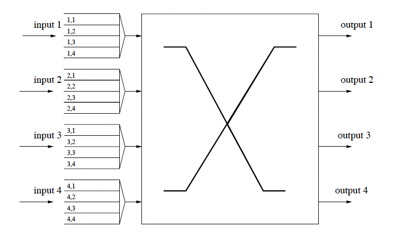
Figure 3: A $4\times 4$ input-queued switch used in a router. Figure taken from hajek2015random.

Problem description: An $N\times N$ input-queued switch has $N$ input ports and $N$ output ports. Each of the $N$ input ports maintains a separate FIFO queue for each output port. The input and output ports are connected in the form of a bipartite network using a high-speed switch fabric (see Figure 3 for a simplified schematic). At any round (also called slots), each input port can be connected to at most one output port for transmitting the packets. The objective of a switching policy is to choose an input-output matching at each round to route the packets from the input queues to their destinations so that the input queue lengths grow sub-linearly with time (i.e., they remain rate-stable (neely2010stochastic)). Please refer to the standard references e.g., hajek2015random and the original papers (tassiulas1990stability; mckeown1999achieving) for a more detailed description of the input-queued switch architectures and constraints.

Admissible actions and the queueing process:

Let $\Omega$ be the set of all $N\times N$ doubly stochastic matrices (a.k.a. the Birkhoff polytope). The set $\Omega$ is known to coincide with the convex hull of all incidence vectors corresponding to the perfect matchings of the $N\times N$ bipartite graph (hajek2015random). At each round, the policy chooses a feasible action $x(t)\equiv\big{(}x_{ij}(t),1\leq i,j\leq N\big{)}$ from the admissible set $\Omega.$ It then randomly samples a matching $z(t)\equiv\big{(}z_{ij}(t)\in\{0,1\},1\leq i,j\leq N\big{)}$ using the Birkhoff-Von-Neumann decomposition, such that $\mathbb{E}z(t)=x(t)$. At the same time, the adversary reveals a packet arrival vector $\bm{b}(t)$ and a service rate vector $\bm{s}(t)$. The arrival and service processes could be binary-valued or could assume any non-negative integers from a bounded range. As a result, the $i$^th input queue length corresponding to the $j$^th output port evolves as follows:

$$Q_{ij}(t)=\big{(}Q_{ij}(t-1)+b_{ij}(t)-s_{ij}(t)z_{ij}(t))^{+},Q_{ij}(0)=0.$$ (38)

$S$-Feasibility:

We assume that the adversary is $S$-feasible, i.e., $\exists x^{*}\in\mathcal{X}$ such that

$$\sum_{t\in\mathcal{I}}(b_{ij}(t)-s_{ij}(t)x^{*}_{ij})\leq 0,\forall i,j,\forall\textrm{sub-intervals}~{}\mathcal{I},|\mathcal{I}|=S.$$

The fixed admissible action $x^{*}$ is unknown to the switching policy. Since we do not assume Slater’s condition, the queue-length bounds derived in neely2017online do not apply here.

Reduction to the OCS problem:

The above scheduling problem can be straightforwardly reduced to the OCS problem where we consider $k=N^{2}$ linear constraints, where the $(i,j)$^th constraint function is defined as

$$g_{t,(ij)}(x)\equiv b_{ij}(t)-s_{ij}x_{ij},~{}1\leq i,j\leq N.$$

It follows that the auxiliary queueing variables in the OCS meta-policy in Algorithm 2 evolve similarly to Eqn. (38). Hence, taking expectation over the randomness of the policy and using arguments exactly similar to the proof of Theorem 5, it follows that under Algorithm 2, each of the $N^{2}$ input queues grows sublinearly as $\mathbb{E}Q_{ij}(t)=O(\max(\sqrt{St},S)),$ where the expectation is taken over the randomness of the policy. Hence, as long as $S$ is a constant, the queues remain rate stable. To exploit the combinatorial structure of the problem, it is computationally advantageous to use the FTPL sub-routine (abernethy2014online, Theorem 11) as the base OCO policy in Algorithm 2, which can be implemented efficiently by a maximum-weight matching oracle and leads to the same queue length bounds.

8 Conclusion and open problems

In this paper, we proposed efficient algorithms for the Online Constraint Satisfaction and the Generalized OCO problems and established tight performance bounds for static regret and cumulative constraint violations. An exciting research direction would be to extend our methodologies to bound the dynamic regret. Investigating the generalized OCO problem with strongly convex constraints would be interesting. Furthermore, obtaining optimal performance bounds with the relaxed $S$-feasible benchmarks for the Generalized OCO problem would be nice. Finally, extending our work to the bandit feedback setting will be of interest (sinha2023banditq).

9 Acknowledgement

The work of AS is partially supported by a US-India NSF-DST collaborative grant coordinated by IDEAS-Technology Innovation Hub (TIH) at the Indian Statistical Institute, Kolkata.

10 Appendix

10.1 Proof of Proposition 1

Upon dividing each term of the sequence $\{Q(t)\}_{t\geq 1}$ by $c,$ without ant loss of generality, we may assume that $c=1$. Hence, from Eqn. (22), we have the following preliminary bound on the growth of the sequence:

$$Q^{2}(t)\stackrel{{\scriptstyle(a)}}{{\leq}}\sum_{\tau=1}^{t}\frac{Q^{2}(\tau)}{Q(\tau)}=\sum_{\tau=1}^{t}Q(\tau),~{}\forall t\geq 1.$$ (39)

where in (a), we have used the fact that each term of the sequence is non-negative. Substituting the bound (39) into the RHS of Eqn. (22), we obtain

$$Q^{2}(t)\leq\sum_{\tau=1}^{t}\frac{\sum_{s=1}^{\tau}Q(s)}{\sum_{s=1}^{\tau}Q(s)}=t.$$

This yields

$$Q(t)\leq\sqrt{t},~{}\forall t\geq 1.$$ (40)

Next, for any fixed $t\geq 1,$ let $\arg\max_{\tau=1}^{t}Q(\tau)=z$ (ties, if any, have been broken arbitrarily). Without any loss of generality, we may assume $Q(z)>0$. Now we have:

$$Q^{2}(z)\stackrel{{\scriptstyle(b)}}{{\leq}}\sum_{\tau=1}^{z}\frac{Q^{2}(\tau)}{\sum_{s=1}^{\tau}Q(s)}\stackrel{{\scriptstyle(c)}}{{\leq}}\sum_{\tau=1}^{t}\frac{Q^{2}(\tau)}{\sum_{s=1}^{\tau}Q(s)}\stackrel{{\scriptstyle(d)}}{{\leq}}Q(z)\sum_{\tau=1}^{t}\frac{Q(\tau)}{\sum_{s=1}^{\tau}Q(s)}$$

where in (b), we have used (22), in (c), we have used the non-negativity of the sequence, and in (d), we have used the fact that $Q(z)\geq Q(\tau),1\leq\tau\leq t.$ Dividing both sides by $Q(z),$ the above inequality yields:

$$Q(z)\leq\sum_{\tau=1}^{t}\frac{Q(\tau)}{\sum_{s=1}^{\tau}Q(s)}.$$

Finally, for any $t\geq 1,$ we have

$$Q(t)\leq Q(z) \leq \sum_{\tau=1}^{t}\frac{Q(\tau)}{\sum_{s=1}^{\tau}Q(s)}$$

$$\leq \sum_{\tau=1}^{t}\int_{\sum_{s=1}^{\tau-1}Q(s)}^{\sum_{s=1}^{\tau}Q(s)}\frac{dx}{x}$$

$$\leq 1+\int_{Q(1)}^{\sum_{s=1}^{t}Q(s)}\frac{dx}{x}$$

$$\stackrel{{\scriptstyle(e)}}{{=}} \ln(\sum_{s=1}^{t}Q(s))+c_{1}$$

$$\stackrel{{\scriptstyle(f)}}{{\leq}} \ln(\sum_{s=1}^{t}\sqrt{s})+c_{1}\leq\frac{3}{2}\ln(t)+c_{1},$$

where in (c), we have defined the constant $c_{1}\equiv 1-\ln(Q(1))$ and in (f), we have used the bound given by Eqn. (40). We can tighten the previous bound further by substituting it in the inequality $(e)$ above, which results in

$$Q(t)\leq\ln(\sum_{s=1}^{t}\frac{3}{2}\ln s+c_{1}t)\leq\ln(t)+\ln(c_{1}+\frac{3}{2}\ln(t)).~{}~{}~{}~{}\blacksquare$$

10.2 Proof of Theorem 3

Bounding the constraint violations:

Since the cost functions are assumed to be Lipschitz with Lipschitz constant $G$ (Assumption 2), we have $\textrm{Regret}_{t}(x^{*})\geq-GDt.$ Hence, from Eqn. (31), we have

$$Q^{2}(t)\leq VG\delta t+2GD\sqrt{\sum_{\tau=1}^{t}Q^{2}(\tau)}.$$ (41)

where we have defined $\delta\equiv D(\frac{1}{V}+\frac{2}{\sqrt{t}})\leq 3D.$ Hence, for all $1\leq\tau\leq t,$ we have

$$Q^{2}(\tau)\leq 3VGDt+2GD\sqrt{\sum_{\tau=1}^{t}Q^{2}(\tau)}.$$

Summing up the above inequalities for $1\leq\tau\leq t,$ we obtain

$$\sum_{\tau=1}^{t}Q^{2}(\tau)\leq 3VGDt^{2}+2GDt\sqrt{\sum_{\tau=1}^{t}Q^{2}(\tau)}.$$

Solving the above quadratic inequality, we conclude

$$\sqrt{\sum_{\tau=1}^{t}Q^{2}(\tau)}\leq t(2GD+\sqrt{3VGD}).$$ (42)

Finally, combining the bound (42) with Eqn. (41), we obtain

$$Q^{2}(t)\leq O(Vt)+O(t\sqrt{V})\implies Q(t)=O(\sqrt{Vt})\stackrel{{\scriptstyle(V=\sqrt{T})}}{{\implies}}Q(t)=O(T^{3/4}).$$

The above concludes the proof of the constraint violation bound as claimed in the theorem. $\blacksquare$

Note:

In the proof above, we have not used the fact that the constraint functions are non-negative. Hence, the above violation bound holds for constraints which are not necessarily pre-processed (see Section 5). However, the remaining part of the proof exploits the non-negativity of the pre-processed constraint functions.

Bounding the regret:

Since the constraint functions are non-negative, the sequence $\{Q(t)\}_{t\geq 1}$ is monotone non-decreasing. Hence, from Eqn. (32), we have

$$V\textrm{Regret}_{t}(x^{*})\leq 2GDQ(t)\sqrt{t}-Q^{2}(t)+2GDV\sqrt{t},$$

where, in the first term on the RHS, we have used the monotonicity of the queue-length sequence. Completing the square on the RHS, we have

$$V\textrm{Regret}_{t}(x^{*}) \leq 2GDV\sqrt{t}+G^{2}D^{2}t-(Q(t)-GD\sqrt{t})^{2}$$ (43)

$$\leq 2GDV\sqrt{t}+G^{2}D^{2}t.$$ (44)

Hence, we conclude that

$$\textrm{Regret}_{t}(x^{*})\leq 2GD\sqrt{t}+\frac{G^{2}D^{2}t}{V}\stackrel{{\scriptstyle(V=\sqrt{T})}}{{\implies}}\textrm{Regret}_{t}(x^{*})=O(\sqrt{t}).~{}\blacksquare$$

Bounding the queue-length when the regret is non-negative:

We now establish the improved queue length bound for rounds where the worst-case regret is non-negative. Consider a round $t\geq 1$ s.t. $\sup_{x^{*}\in\Omega^{*}}\textrm{Regret}_{t}(x^{*})\geq 0.$ From Eqn. (43), we have

$$(Q(t)-GD\sqrt{t})^{2}\leq 2GDV\sqrt{t}+G^{2}D^{2}t.$$

This yields

$$Q(t)\leq GD\sqrt{t}+\sqrt{2GDV\sqrt{t}}+GD\sqrt{t}.$$

Setting $V=\sqrt{T},$ the above bound yields

$$Q(t)=O((Tt)^{1/4})+O(\sqrt{t})=O(\sqrt{T}),~{}\forall t\geq 1.~{}~{}~{}~{}\blacksquare$$

10.3 Proof of Theorem 4

Bounding the constraint violations:

Since the pre-processed (clipped) constraint functions are non-negative, the queue length sequence is monotone non-decreasing. Hence, from Eqn. (32), we have

$$Q^{2}(t)+V\textrm{Regret}_{t}(x^{*})\leq\frac{VG^{2}}{\alpha}\ln(t)+\frac{G^{2}}{\alpha V}Q^{2}(t)\ln(T),$$ (45)

where, on the last term in the RHS, we have used the non-decreasing property of the queue lengths and the fact that $t\leq T$. Setting $V=\frac{2G^{2}\ln(T)}{\alpha},$ and transposing the last term on the RHS to the left, the above inequality yields

$$Q^{2}(t)+2V\textrm{Regret}_{t}(x^{*})\leq\frac{2VG^{2}}{\alpha}\ln(t).$$ (46)

Since the cost functions are assumed to be Lipschitz with Lipschitz constant $G$ (Assumption 2), we have $\textrm{Regret}_{t}(x^{*})\geq-GDt.$ Hence, from Eqn. (46), we have

$$Q^{2}(t)\leq 2VGDt+\frac{2VG^{2}}{\alpha}\ln(t)\stackrel{{\scriptstyle(V=\frac{2G^{2}\ln(T)}{\alpha})}}{{\implies}}Q(t)=O\big{(}\sqrt{\frac{t\log T}{\alpha}}\big{)}.~{}~{}~{}~{}\blacksquare$$

Bounding the regret:

Since $Q^{2}(t)\geq 0,$ from Eqn. (46), we have

$$2V\textrm{Regret}_{t}(x^{*})\leq\frac{2VG^{2}}{\alpha}\ln(t),$$

where we have set $V=\frac{2G^{2}\ln(T)}{\alpha}.$ This leads to the following logarithmic regret-bound

$$\textrm{Regret}_{t}(x^{*})\leq\frac{G^{2}}{\alpha}\ln(t).~{}~{}~{}~{}\blacksquare$$

Bounding the queue length when the regret is non-negative:

As in the convex case, we now establish an improved queue length bound for any round $t\geq 1$ where the worst-case regret is non-negative. Let $\sup_{x^{*}\in\Omega^{*}}\textrm{Regret}_{t}(x^{*})\geq 0$ for some round $t\geq 1.$ Letting $V=\frac{2G^{2}\ln(T)}{\alpha},$ from Eqn. (46), we have

$$Q^{2}(t)\leq\frac{2VG^{2}}{\alpha}\ln(t)\implies Q(t)=O(\frac{\ln T}{\alpha}).~{}\blacksquare$$

10.4 Proof of Theorem 5

We now specialize the generalized regret decomposition bound in (37) to the case of convex constraints. Using the OGD policy with adaptive step-sizes given in part 1 of Theorem 1, we have

$$\sum_{i=1}^{k}Q_{i}^{2}(t)\leq c_{1}\sqrt{\sum_{\tau=1}^{t}\big{(}\sum_{i=1}^{k}Q_{i}^{2}(\tau)\big{)}}+c_{2}St+c_{3}S\sum_{i=1}^{k}Q_{i}(t)+c_{4}S^{2}$$

where the constants $c_{1}\equiv O(GD\sqrt{k}),c_{2}=O(kF^{2}),c_{3}=O(F),c_{4}=O(kF^{2})$ are problem-specific parameters that depend on the bounds on the gradients and the value of the constraints, the number of constraints, and the diameter of the admissible set. Using Cauchy-Schwarz inequality on the penultimate term on the RHS and defining $Q^{2}(t)\equiv\sum_{i}Q_{i}^{2}(t),$ we obtain:

$$Q^{2}(t)\leq c_{1}\sqrt{\sum_{\tau=1}^{t}Q^{2}(\tau)}+c_{2}St+c_{3}^{\prime}SQ(t)+c_{4}S^{2}.$$

Since $Q(t)\leq Ft,$ the above inequality can be simplified to

$$Q^{2}(t)\leq c_{1}\sqrt{\sum_{\tau=1}^{t}Q^{2}(\tau)}+c_{2}^{\prime}St+c_{4}S^{2},~{}\forall t\geq 1,$$ (47)

where we have defined $c_{2}^{\prime}\equiv c_{3}^{\prime}F+c_{2}.$ To solve the above system of inequalities, note that for each $1\leq\tau\leq t,$ we have

$$Q^{2}(\tau)\leq c_{1}\sqrt{\sum_{\tau=1}^{t}Q^{2}(\tau)}+c_{2}^{\prime}St+c_{4}S^{2}.$$

Summing up the above inequalities for $1\leq\tau\leq t$ and defining $Z_{t}\equiv\sqrt{\sum_{\tau=1}^{t}Q^{2}(\tau)},$ we obtain

$$Z^{2}_{t} \leq c_{1}tZ_{t}+c_{2}^{\prime}St^{2}+c_{4}S^{2}t$$

$$\emph{i.e.,}~{}Z_{t}^{2} \leq 3\max(c_{1}tZ_{t},c_{2}^{\prime}St^{2},c_{4}S^{2}t)$$

$$\emph{i.e.,}~{}Z_{t} = O(\max(t,t\sqrt{S},S\sqrt{t})).$$

Substituting the above bound for $Z(t)$ in Eqn.  (47), we have:

$$Q^{2}(t) = O(\max(Z_{t},St,S^{2}))$$

$$\emph{i.e.,}~{}Q(t) = O(\max(\sqrt{Z_{t}},\sqrt{St},S))$$

$$\textrm{Hence,}~{}~{}Q_{i}(t)\leq Q(t) = O(\max(\sqrt{t},\sqrt{t}S^{1/4},\sqrt{S}t^{1/4},\sqrt{St},S))$$

$$= O(\max(\sqrt{St},S)),~{}\forall i\in[k].~{}~{}~{}~{}\blacksquare$$

References

- Liakopoulos et al. (2019) Nikolaos Liakopoulos, Apostolos Destounis, Georgios Paschos, Thrasyvoulos Spyropoulos, and Panayotis Mertikopoulos. Cautious regret minimization: Online optimization with long-term budget constraints. In Kamalika Chaudhuri and Ruslan Salakhutdinov, editors, Proceedings of the 36th International Conference on Machine Learning, volume 97 of Proceedings of Machine Learning Research, pages 3944–3952. PMLR, 09–15 Jun 2019. URL https://proceedings.mlr.press/v97/liakopoulos19a.html.
- Sinha (2023) Abhishek Sinha. BanditQ - Fair Multi-Armed Bandits with Guaranteed Rewards per Arm. arXiv preprint arXiv:2304.05219, 2023.
- Zinkevich (2003) Martin Zinkevich. Online convex programming and generalized infinitesimal gradient ascent. In Proceedings of the 20th international conference on machine learning (icml-03), pages 928–936, 2003.
- Hazan et al. (2007) Elad Hazan, Alexander Rakhlin, and Peter Bartlett. Adaptive online gradient descent. Advances in neural information processing systems, 20, 2007.
- Orabona and Pál (2018) Francesco Orabona and Dávid Pál. Scale-free online learning. Theoretical Computer Science, 716:50–69, 2018.
- Orabona (2019) Francesco Orabona. A modern introduction to online learning. arXiv preprint arXiv:1912.13213, 2019.
- Yuan and Lamperski (2018) Jianjun Yuan and Andrew Lamperski. Online convex optimization for cumulative constraints. Advances in Neural Information Processing Systems, 31, 2018.
- Jenatton et al. (2016) Rodolphe Jenatton, Jim Huang, and Cédric Archambeau. Adaptive algorithms for online convex optimization with long-term constraints. In International Conference on Machine Learning, pages 402–411. PMLR, 2016.
- Yu et al. (2017) Hao Yu, Michael Neely, and Xiaohan Wei. Online convex optimization with stochastic constraints. Advances in Neural Information Processing Systems, 30, 2017.
- Yu and Neely (2016) Hao Yu and Michael J Neely. A low complexity algorithm with regret and constraint violations for online convex optimization with long term constraints. arXiv preprint arXiv:1604.02218, 2016.
- Mahdavi et al. (2012) Mehrdad Mahdavi, Rong Jin, and Tianbao Yang. Trading regret for efficiency: online convex optimization with long term constraints. The Journal of Machine Learning Research, 13(1):2503–2528, 2012.
- Yi et al. (2021) Xinlei Yi, Xiuxian Li, Tao Yang, Lihua Xie, Tianyou Chai, and Karl Johansson. Regret and cumulative constraint violation analysis for online convex optimization with long term constraints. In International Conference on Machine Learning, pages 11998–12008. PMLR, 2021.
- Guo et al. (2022) Hengquan Guo, Xin Liu, Honghao Wei, and Lei Ying. Online convex optimization with hard constraints: Towards the best of two worlds and beyond. Advances in Neural Information Processing Systems, 35:36426–36439, 2022.
- Neely and Yu (2017) Michael J Neely and Hao Yu. Online convex optimization with time-varying constraints. arXiv preprint arXiv:1702.04783, 2017.
- Sun et al. (2017) Wen Sun, Debadeepta Dey, and Ashish Kapoor. Safety-aware algorithms for adversarial contextual bandit. In Doina Precup and Yee Whye Teh, editors, Proceedings of the 34th International Conference on Machine Learning, volume 70 of Proceedings of Machine Learning Research, pages 3280–3288. PMLR, 06–11 Aug 2017. URL https://proceedings.mlr.press/v70/sun17a.html.
- Yi et al. (2023) Xinlei Yi, Xiuxian Li, Tao Yang, Lihua Xie, Yiguang Hong, Tianyou Chai, and Karl H Johansson. Distributed online convex optimization with adversarial constraints: Reduced cumulative constraint violation bounds under slater’s condition. arXiv preprint arXiv:2306.00149, 2023.
- Liu et al. (2022) Qingsong Liu, Wenfei Wu, Longbo Huang, and Zhixuan Fang. Simultaneously achieving sublinear regret and constraint violations for online convex optimization with time-varying constraints. ACM SIGMETRICS Performance Evaluation Review, 49(3):4–5, 2022.
- Meyn (2008) Sean Meyn. Control techniques for complex networks. Cambridge University Press, 2008.
- Neely (2010) Michael J Neely. Stochastic network optimization with application to communication and queueing systems. Synthesis Lectures on Communication Networks, 3(1):1–211, 2010.
- Rockafellar (1972) R. Tyrrel Rockafellar. Convex Analysis. Princeton University Press, Princeton, New Jersey, 1972.
- Hazan et al. (2016) Elad Hazan et al. Introduction to online convex optimization. Foundations and Trends® in Optimization, 2(3-4):157–325, 2016.
- Abernethy et al. (2014) Jacob Abernethy, Chansoo Lee, Abhinav Sinha, and Ambuj Tewari. Online linear optimization via smoothing. In Conference on Learning Theory, pages 807–823, 2014.
- Joulani et al. (2016) Pooria Joulani, Andras Gyorgy, and Csaba Szepesvári. Delay-tolerant online convex optimization: Unified analysis and adaptive-gradient algorithms. In Proceedings of the AAAI Conference on Artificial Intelligence, volume 30, 2016.
- Ruder (2017) Sebastian Ruder. An overview of multi-task learning in deep neural networks. arXiv preprint arXiv:1706.05098, 2017.
- Dekel et al. (2006) Ofer Dekel, Philip M Long, and Yoram Singer. Online multitask learning. In International Conference on Computational Learning Theory, pages 453–467. Springer, 2006.
- Murugesan et al. (2016) Keerthiram Murugesan, Hanxiao Liu, Jaime Carbonell, and Yiming Yang. Adaptive smoothed online multi-task learning. Advances in Neural Information Processing Systems, 29, 2016.
- Jun et al. (2017) Kwang-Sung Jun, Francesco Orabona, Stephen Wright, and Rebecca Willett. Improved strongly adaptive online learning using coin betting. In Artificial Intelligence and Statistics, pages 943–951. PMLR, 2017.
- Asmussen (2003) Søren Asmussen. Applied probability and queues, volume 2. Springer, 2003.
- McKeown et al. (1999) Nick McKeown, Adisak Mekkittikul, Venkat Anantharam, and Jean Walrand. Achieving 100% throughput in an input-queued switch. IEEE Transactions on Communications, 47(8):1260–1267, 1999.
- Tassiulas and Ephremides (1990) Leandros Tassiulas and Anthony Ephremides. Stability properties of constrained queueing systems and scheduling policies for maximum throughput in multihop radio networks. In 29th IEEE Conference on Decision and Control, pages 2130–2132. IEEE, 1990.
- Hajek (2015) Bruce Hajek. Random processes for engineers. Cambridge university press, 2015.