TIC-TAC: A framework to Learn and Evaluate Your Covariance

Abstract

We study the problem of unsupervised heteroscedastic covariance estimation, where the goal is to learn the multivariate target distribution $\mathcal{N}(\displaystyle{\bm{y}},\displaystyle{\bm{\Sigma}}_{y}|\displaystyle{\bm{x}})$ given an observation $\displaystyle{\bm{x}}$. This problem is particularly challenging as $\displaystyle{\bm{\Sigma}}_{{\bm{y}}}$ varies for different samples (heteroscedastic) and no annotation for the covariance is available (unsupervised). Typically, state-of-the-art methods predict the mean $\displaystyle f_{\theta}({\bm{x}})$ and covariance $\displaystyle\mathrm{Cov}(f_{\theta}({\bm{x}}))$ of the target distribution through two neural networks trained using the negative log-likelihood. This raises two questions: (1) Does the predicted covariance truly capture the randomness of the predicted mean? (2) In the absence of ground-truth annotation, how can we quantify the performance of covariance estimation? We address (1) by deriving TIC: Taylor Induced Covariance, which captures the randomness of the multivariate $\displaystyle f_{\theta}({\bm{x}})$ by incorporating its gradient and curvature around ${\bm{x}}$ through the second order Taylor polynomial. Furthermore, we tackle (2) by introducing TAC: Task Agnostic Correlations, a metric which leverages conditioning of the normal distribution to evaluate the covariance. We verify the effectiveness of TIC through multiple experiments spanning synthetic (univariate, multivariate) and real-world datasets (UCI Regression, LSP, and MPII Human Pose Estimation). Our experiments show that TIC outperforms state-of-the-art in accurately learning the covariance, as quantified through TAC.

1 Introduction

Modeling the target distribution $p({\bm{y}}|{\bm{x}})$ for a pair of input-target samples (${\bm{x}},{\bm{y}}$) is an important design choice in regression analysis. The standard assumption is that $p({\bm{y}}|{\bm{x}})$ follows a multivariate normal distribution $\mathcal{N}({\bm{y}},{\bm{\Sigma}}_{y}|{\bm{x}})$, where the target ${\bm{y}}$ corresponds to the mean of this distribution. The challenge with covariance estimation is that while training samples (${\bm{x}},{\bm{y}}$) are observed, ${\bm{\Sigma}}_{y}$ needs to be inferred. Indeed, it is significantly easier to obtain annotations for (${\bm{x}},{\bm{y}}$) in comparison to ${\bm{\Sigma}}_{y}$, making covariance estimation an unsupervised task. Moreover, ${\bm{\Sigma}}_{y}$ is often heteroscedastic and takes on different values for different input samples. Regressing ${\bm{x}}$ to ${\bm{y}}$ can be simplified by assuming the covariance to be an identity matrix, ${\bm{\Sigma}}_{y}=\displaystyle{\bm{I}}_{n}$, or ignoring correlations (${\bm{\Sigma}}_{y}=\text{diag}(\sigma)$). However, such approaches diminish the main advantages of learning the covariance, such as correlation analysis, sampling from $\mathcal{N}({\bm{y}},{\bm{\Sigma}}_{y}\,|\,{\bm{x}})$, and updating our estimates conditioned on partial observations of the target $\mathcal{N}(\tilde{{\bm{y}}}_{[k:n]},{\bm{\Sigma}}_{y}\,|\,{\bm{x}},{\bm{y}}_{[1:k]})$.

Typically, covariance estimation is performed through minimizing the negative log-likelihood of the target distribution. This involves the joint optimization of a target $\hat{{\bm{y}}}=f_{\theta}({\bm{x}})$ and a covariance $\mathrm{Cov}(\hat{{\bm{y}}})=g_{\Theta}({\bm{x}})$ estimator (Dorta et al., 2018). However, state-of-the-art results (Seitzer et al., 2022; Stirn et al., 2023) show that this joint optimization of $f_{\theta}$ and $g_{\Theta}$ causes sub-optimal target $\hat{{\bm{y}}}$ predictions because of incorrect covariance $\mathrm{Cov}(\hat{{\bm{y}}})$ predictions. Indeed, in the absence of supervision, $\mathrm{Cov}(\hat{{\bm{y}}})=g_{\Theta}({\bm{x}})$ is essentially an arbitrary mapping of every ${\bm{x}}$ to a positive definite matrix that minimizes the objective. As a result, $\mathrm{Cov}(\hat{{\bm{y}}})$ may not truly explain the randomness in $\hat{{\bm{y}}}$. Moreover, assessing the quality of covariance estimation is challenging without ground-truth labels. Optimization metrics such as likelihood scores are not a direct measure of the accuracy of the correlations learnt by the covariance estimator since they also incorporate the performance of the mean estimator. For instance, the mean square error would be zero for the perfect estimator $f_{\theta}(x)$, and completely disregard the covariance. Alternative measure such as log-likelihood put greater emphasis on the determinant of the covariance without directly assessing the covariance. Therefore, we distill the challenges associated with covariance estimation into two problem statements: (1) How do we formulate $\mathrm{Cov}(\hat{{\bm{y}}})$ to explain the randomness in $\hat{{\bm{y}}}$? (2) How do we assess the quality of covariance estimation in the absence of ground-truth annotations?

Our first major contribution, the Taylor Induced Covariance (TIC), explains the randomness in $f_{\theta}({\bm{x}})$ through a novel derivation of a closed form expression for $\mathrm{Cov}(f_{\theta}({\bm{x}}))$. Specifically, we derive this expression by solving for the covariance of the multivariate target $f_{\theta}({\bm{x}}+\epsilon)$ through its Taylor expansion around ${\bm{x}}$. As a result we can model the covariance through the gradient and curvature of $f_{\theta}({\bm{x}})$ which captures the variation in the prediction within an $\epsilon$-neighborhood of ${\bm{x}}$.

Our second major contribution, the Task Agnostic Correlations (TAC), addresses the lack of a direct metric to estimate the quality of covariance estimation. By definition, an accurate covariance prediction correctly estimates the correlations underlying the target random variables. Hence, given a partial observation of the target ${\bm{y}}_{[1:k]}$, the covariance should accurately update the prediction $\tilde{{\bm{y}}}_{[k:n]}$ towards the unobserved target ${\bm{y}}_{[k:n]}$ based on conditioning of the target distribution $\mathcal{N}(\tilde{{\bm{y}}}_{[k:\texttt{n}]},\mathrm{Cov}(\hat{{\bm{y}}})\,|\,{\bm{x}},{\bm{y}}_{[1:\texttt{k}]})$. Subsequently, we quantify TAC as the conditional mean absolute error between the updated prediction and the unobserved target.

We design and perform extensive experiments on synthetic (sinusoidal, multivariate) and real-world datasets (UCI Regression and Human Pose - MPII, LSP), across fully-connected and convolutional network architectures. Using TAC, our experiments show that TIC outperforms state-of-the-art baselines in learning correlations across all tasks and architectures, demonstrating the effectiveness of our method for unsupervised heteroscedastic covariance estimation. We make TIC-TAC’s code publicly available at: www.github.com/vita-epfl/TIC-TAC
We briefly describe below the notation which will be used throughout the paper:

Description	Networks	Target	Prediction	Shape	Is Target Known?
Mean Estimator	$f_{\theta}({\bm{x}})$	${\bm{y}}$	$\hat{{\bm{y}}}$	$\mathbb{R}^{n}$	Yes
Covariance Estimator	$g_{\Theta}({\bm{x}})$	${\bm{\Sigma}}_{{\bm{y}}}$	$\mathrm{Cov}(f_{\theta}({\bm{x}}))$	$\mathbb{R}^{n\times n}$	No

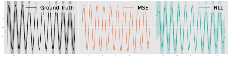
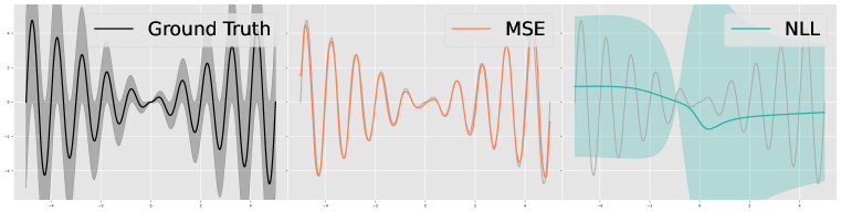
Figure 2: (Left) In the absence of supervision, $\mathrm{Cov}(\hat{{\bm{y}}})=g_{\Theta}({\bm{x}})$ is essentially an arbitrary mapping of every ${\bm{x}}$ to a positive definite matrix that minimizes the likelihood. As a result, $\mathrm{Cov}(\hat{{\bm{y}}})$ may not truly explain the randomness in $\hat{{\bm{y}}}$. (Right) In contrast, the Taylor Induced Covariance (TIC) explains the randomness in $\hat{{\bm{y}}}$ through the gradient and curvature of the mean estimator ${\bm{y}}=f_{\theta}({\bm{x}})$. Intuitively, the gradient and curvature quantify the variation in the prediction within an $\epsilon$-neighborhood of ${\bm{x}}$.

2 Related Work

Negative Log-Likelihood Based Approaches: In the absence of annotation, the most widely used approach (Dorta et al., 2018; Gundavarapu et al., 2019; Russell & Reale, 2021; Lu & Koniusz, 2022; Simpson et al., 2022; Liu et al., 2018; Barratt & Boyd, 2022; Kendall & Gal, 2017) for covariance estimation is to perform negative log-likelihood based optimization. Typically, this involves a mean $\hat{{\bm{y}}}=f_{\theta}({\bm{x}})$ and covariance $\mathrm{Cov}(\hat{{\bm{y}}})=g_{\Theta}({\bm{x}})$ estimator which are trained to minimize the objective

$$\hat{\theta},\hat{\Theta}=\operatorname*{arg\,min}_{\theta,\Theta}\,\,\,\,\,\,\,\,\,\log|\mathrm{Cov}(\hat{{\bm{y}}})|+({\bm{y}}-\hat{{\bm{y}}})^{T}\,\,\mathrm{Cov}(\hat{{\bm{y}}})^{-1}\,\,({\bm{y}}-\hat{{\bm{y}}})\;.$$

Recent studies (Seitzer et al., 2022) in negative log-likelihood show that this formulation results in suboptimal fits due to the incorrect scaling of the residual ${\bm{y}}-f_{\theta}({\bm{x}})$ by the standard deviation $\sigma_{\Theta}({\bm{x}})$. Subsequently, Seitzer et al. (2022) propose $\beta$-NLL, which addresses this by reducing the impact of the predicted standard deviation in the training process. Specifically, $\beta$-NLL introduces a new term $\sigma^{2\beta}$ to the negative log-likelihood as

$$\hat{\theta},\hat{\Theta}=\operatorname*{arg\,min}_{\theta,\Theta}\,\,\,\,\,\,\,\,\,\lfloor\hat{\sigma}^{2\beta}_{\Theta}(x)\rfloor\,\,\bigg{[}\log|\hat{\sigma}^{2}_{\Theta}(x)|+\frac{(y-f_{\theta}(x))^{2}}{\hat{\sigma}^{2}_{\Theta}(x)}\bigg{]}.$$

Intuitively, any $\beta\neq\{0,1\}$ provides a degree of trade-off between the negative log-likelihood objective and the mean squared error. While $\beta$-NLL is delightfully simple and effective, we argue that this method has key limitations. First, $\beta$-NLL is not a result of a valid distribution, and the values that are optimized for do not translate to the true variance of the distribution. Second, $\beta$-NLL is a scaled variant of the negative log-likelihood; samples that are inherently noisy take larger gradient steps in comparison to clean samples, leading to imbalanced convergence. The recent method of Stirn et al. (2023) proposes an alternative approach and allows the target estimator to converge faster by training it with identity covariance. However, this involves conflicting assumptions; while the target estimator assumes that variables within ${\bm{y}}-f_{\theta}({\bm{x}})$ are uncorrelated, the covariance estimator is expected to recover correlations from the residual.

Finally, the drawback of $\mathrm{Cov}(\hat{{\bm{y}}})=g_{\Theta}({\bm{x}})$ being an arbitrary mapping from ${\bm{x}}$ to a positive definite matrix is common to all the aforementioned approaches. This drawback is significant since in the absence of supervision, $g_{\Theta}({\bm{x}})$ can take on any value which minimizes the objective as shown in Seitzer et al. (2022), and does not necessarily represent the randomness of the prediction. Therefore, we derive a closed form expression for the covariance $\mathrm{Cov}(\hat{{\bm{y}}})$ and show that incorporating the gradient and curvature better explains the randomness in $\hat{{\bm{y}}}$.

Probabilistic Methods: Gaussian Process (Le et al., 2005) is a powerful tool for probabilistic modeling of data. However, it does not model the covariance and instead uses a positive definite kernel which quantifies the similarity between various samples. The statistical properties of covariance have been well explored in the community (Biswas et al., 2020; Hoff et al., 2022; Kastner, 2019; Nguyen et al., 2022), however, the motivation of this work is different. We place less emphasis on statistics with more emphasis on obtaining a covariance approximation to define the conditional distribution over the target given a sample. For instance, works such as Chen et al. (2017), aim to reduce the time complexity of computing the covariance by introducing elements from compressive sensing. However, the method does not naturally extrapolate to our framework where we wish to learn heteroscedastic covariance conditioned on the input samples. Ensembles are useful in computing epistemic uncertainty Kendall & Gal (2017); Lakshminarayanan et al. (2017), however the method quantifies the disagreement over the target and does not represent the correlations within the target. The Taylor series has previously been applied in a different problem of propagating uncertainty in measurement theory. However the analysis is limited to univariate targets (ISO & OIML, 1995–2020; Kirkup & Frenkel, 2006) or provides a numerical solution (Gu et al., 2021) to estimating the covariance. In contrast, we propose a novel derivation and optimization of a closed form expression for heteroscedastic covariance estimation.

Hessians in Deep Learning: The hessian is interpreted as the curvature of the loss landscape and is significant in optimization Gilmer et al. (2022). Approaches that study uncertainty and optimization using the parameters’ gradients include Jacot et al. (2018); Van Amersfoort et al. (2020). The duality between gradient and hessian has been well studied through the Fisher information (Ly et al., 2017) and applied in uncertainty estimation (Shukla, 2022). Of particular importance is the Cramer-Rao bound which is used in multiple optimizers such as Adam (Kingma & Ba, 2015). Classical (Kanazawa & Kanatani, 2003) and recent (Tirado-Garín et al., 2023) works in the domain of image processing use the Cramer-Rao bound to compute two dimensional covariances based on the heatmap of image descriptors. However, the Cramer-Rao bound estimates the variance of the parametric estimator, and cannot be used to estimate the covariance of the prediction. This limitation cannot be circumvented since Fisher information averages the network gradient over all samples, losing the ability to estimate the covariance for each sample. Therefore, we derive the covariance through a first principles’ approach by attempting to solve for $\mathrm{Cov}(f_{\theta}({\bm{x}}))$ directly.

3 TIC: Taylor Induced Covariance

Let us now introduce our approach to modeling and learning covariance. To this end, we take a step back and ponder on a fundamental question: What is $\mathrm{Cov}({\bm{y}}|{\bm{x}})$? Indeed, $\mathrm{Cov}({\bm{y}}|{\bm{x}})$ is the measure of randomness in ${\bm{y}}$ conditioned on the observation ${\bm{x}}$. However, this definition has subtle differences for discrete and continuous distributions. While the exact value of ${\bm{x}}$ can be observed for discrete distributions, definitions for continuous distributions are inherently based on limits. Therefore, for a continuous distribution, $\mathrm{Cov}({\bm{y}}|{\bm{x}})$ is in fact a shorthand notation for $\mathrm{Cov}(\lim_{\epsilon\rightarrow 0}{\bm{y}}|{\bm{x}}+\epsilon)$. Since $y=f_{\theta}({\bm{x}})$, we have

$$\mathrm{Cov}({\bm{y}}|{\bm{x}}) =\mathrm{Cov}(\lim_{\epsilon\rightarrow 0}f_{\theta}({\bm{x}}+\epsilon)\,|\,{\bm{x}}+\epsilon)$$

$$=\mathrm{Cov}(\lim_{\epsilon\rightarrow 0}f_{\theta}({\bm{x}}+\epsilon)\,|\,{\bm{x}})\;.$$ (1)

Intuitively, Eq. 1 allows us to represent the covariance as the change in ${\bm{y}}$ within an $\epsilon$-neighborhood around ${\bm{x}}$. We can analyze the behavior of $f_{\theta}({\bm{x}}+\epsilon)$ further by taking its Taylor expansion.

3.1 Multivariate Taylor Expansion

The Taylor expansion introduces the notion of curvature in modeling the covariance, and quantifies the rate at which a function can change within a small neighborhood around ${\bm{x}}$. The multivariate Taylor expansion in a matrix notation is given by

$$f_{\theta}({\bm{x}}+\epsilon) \approx f_{\theta}({\bm{x}})+{\bm{J}}({\bm{x}})\epsilon^{T}+\frac{{\bm{h}}}{2}\;, \text{where }{\bm{h}}_{i}=\epsilon\,{\bm{\mathsfit{H}}}_{i}({\bm{x}})\epsilon^{T}\,\,\,\forall i\in 1\dots n\;.$$ (2)

Here, $f_{\theta}(x)\in\mathbb{R}^{n}$ represents the multivariate prediction, $\epsilon\in\mathbb{R}^{m}$ represents the neighborhood of ${\bm{x}}$, ${\bm{J}}({\bm{x}})\in\mathbb{R}^{n\times m}$ corresponds to the Jacobian matrix and ${\bm{\mathsfit{H}}}({\bm{x}})\in\mathbb{R}^{n\times m\times m}$ represents the hessian tensor. Note that all the individual terms in Eq. 2 are $n$-dimensional.

3.2 Covariance Estimation

We interpret the neighborhood $\lim_{\epsilon\rightarrow 0}$ in Eq. 2 as a zero-mean isotropic gaussian distribution $\mathcal{N}(0,\sigma^{2}({\bm{x}}){\bm{I}}_{m})$. While the spread of this random variable is unknown, we assume heteroscedasticity which allows us to represent neighborhoods of varying spatial extents for each ${\bm{x}}$. Introducing stochasticity through the neighborhood allows us to formulate the covariance as a function of the gradient and curvature. The covariance of Eq. 1 with respect to the random variable $\epsilon$ is given by

$$\mathrm{Cov}f_{\theta}({\bm{x}}+\epsilon) =\mathrm{Cov}\bigg{[}f_{\theta}({\bm{x}})+{\bm{J}}({\bm{x}})\epsilon^{T}+\frac{{\bm{h}}}{2}\bigg{]}$$

$$=\mathrm{Cov}\bigg{[}{\bm{J}}({\bm{x}})\epsilon^{T}+\frac{{\bm{h}}}{2}\bigg{]}$$

$$=\mathrm{Cov}({\bm{J}}({\bm{x}})\epsilon^{T})+\mathrm{Cov}(\frac{{\bm{h}}}{2})+2\,\bigg{[}\mathrm{Cov}({\bm{J}}({\bm{x}})\epsilon^{T},\frac{{\bm{h}}}{2})\bigg{]}\;.$$ (3)

We now estimate individual terms in Eq. 3.

Input: ${\bm{y}}$: Ground truth

Input: $\hat{{\bm{y}}}$: Target prediction

Input: $\mathrm{Cov}f_{\theta}({\bm{x}})$: Covariance prediction

Output: TAC: Task Agnostic Correlations metric

1 dimensions = get_dimensions($\hat{{\bm{y}}}$)

2 TAC = zeros(shape=dimensions)

3 for i in dimensions do

4       obs_dim = set(dimensions) - set(i)

5       hidden_dim = i

6       ${\bm{\Sigma}}_{22}$ = $\mathrm{Cov}f_{\theta}({\bm{x}})$[obs_dim, obs_dim]

7       ${\bm{\Sigma}}_{12}$ = $\mathrm{Cov}f_{\theta}({\bm{x}})$[hidden_dim, obs_dim]

8        $\tilde{{\bm{y}}}$ = $\hat{{\bm{y}}}$[hidden_dim] + (${\bm{\Sigma}}_{12}{\bm{\Sigma}}_{22}^{-1}$ (${\bm{y}}[\textrm{obs\_dim}]-\hat{{\bm{y}}}[\textrm{obs\_dim}]$))

9       TAC[i] = $|\tilde{{\bm{y}}}-{\bm{y}}[\textrm{hidden\_dim}]|$

10      

return TAC.mean()

Algorithm 1 TAC: Task Agnostic Correlations

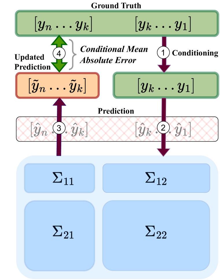
Figure 3: We propose TAC: Task Agnostic Correlations as a metric to assess the quality of covariance estimation. Given the ground truths, predicted mean and the predicted covariance matrix, TAC quantifies the improvement in the predicted mean given partial observations of the ground truth. TAC uses conditioning of the normal distribution as a direct measure to assess the quality of covariance.

3.2.1 Estimating $\mathrm{Cov}({\bm{J}}({\bm{x}})\epsilon^{T},{\bm{h}}/2)$

We note that ${\bm{J}}({\bm{x}})\epsilon^{T}$ and ${\bm{h}}$ are $n$-dimensional vectors with elements $[\dots\bm{J}_{i}({\bm{x}})\epsilon^{T}\dots]$ and $[\dots\epsilon\,{\bm{\mathsfit{H}}}_{k}({\bm{x}})\epsilon^{T}\dots]$ respectively. The covariance between any two elements is given by

$$\mathrm{Cov}\big{(}{\bm{J}}_{i}({\bm{x}})\epsilon^{T},\epsilon\,{\bm{\mathsfit{H}}}_{k}({\bm{x}})\epsilon^{T}\big{)} =\mathbb{E}\big{(}{\bm{J}}_{i}({\bm{x}})\epsilon^{T}\epsilon\,{\bm{\mathsfit{H}}}_{k}({\bm{x}})\epsilon^{T}\big{)}-\mathbb{E}\big{(}{\bm{J}}_{i}({\bm{x}})\epsilon^{T}\big{)}\mathbb{E}\big{(}\epsilon\,{\bm{\mathsfit{H}}}_{k}({\bm{x}})\epsilon^{T}\big{)}$$

$$=\mathbb{E}\big{(}{\bm{J}}_{i}({\bm{x}})\epsilon^{T}\epsilon\,{\bm{\mathsfit{H}}}_{k}({\bm{x}})\epsilon^{T}\big{)}$$

$$=0\;.$$ (4)

We use the property of odd-even functions (Shynk, 2012) to arrive at our solution. We quickly recall that an odd function is defined as $f(-\epsilon)=-f(\epsilon)$ and an even function $f(-\epsilon)=f(\epsilon)$. Furthermore, the random variable $\epsilon$ is an even function since it is zero-mean and symmetric. Next, we note that the product of an odd and even function is odd, and the expectation of an odd function is zero if the underlying probability distribution is an even function as in our case. Finally, the dot product ${\bm{J}}_{i}({\bm{x}})\epsilon^{T}$ can be written as $\sum_{k}{\bm{J}}_{i,k}({\bm{x}})\epsilon^{T}_{k}$. We note that the term $\sum_{k}{\bm{J}}_{i,k}({\bm{x}})\epsilon^{T}_{k}$ is an odd function since $\epsilon$ is symmetric around the origin. Therefore, the expected value of this term is zero.

The term, $\mathbb{E}\big{(}{\bm{J}}_{i}({\bm{x}})\epsilon^{T}\epsilon\,{\bm{\mathsfit{H}}}_{k}({\bm{x}})\epsilon^{T}\big{)}$ can be separated into odd ${\bm{J}}_{i}({\bm{x}})\epsilon^{T}$ and even components $\epsilon\,{\bm{\mathsfit{H}}}_{k}({\bm{x}})\epsilon^{T}$ which are centred around the origin. Therefore, using the property of odd-even functions, $\mathbb{E}\big{(}{\bm{J}}_{i}({\bm{x}})\epsilon^{T}\epsilon\,{\bm{\mathsfit{H}}}_{k}({\bm{x}})\epsilon^{T}\big{)}=0$. As a result, we get $\mathrm{Cov}\big{(}{\bm{J}}_{i}({\bm{x}})\epsilon^{T},\epsilon\,{\bm{\mathsfit{H}}}_{k}({\bm{x}})\epsilon^{T}\big{)}$ = 0 $\forall i,k$, implying that $\mathrm{Cov}({\bm{J}}({\bm{x}})\epsilon^{T},{\bm{h}}/2)=0$.

3.2.2 Estimating $\mathrm{Cov}({\bm{J}}({\bm{x}})\epsilon^{T})$ and $\mathrm{Cov}({\bm{h}}/2)$

Estimating $\mathrm{Cov}({\bm{J}}({\bm{x}})\epsilon^{T})$ and $\mathrm{Cov}({\bm{h}}/2)$ in Eq. 3 is easier since they follow a linear and quadratic form respectively with known solutions for isotropic Gaussian random variables (Eq. 375, 379 in (Petersen & Pedersen, 2012)). Specifically, we have

$$\mathrm{Cov}({\bm{J}}({\bm{x}})\,\,\epsilon^{T}) =k_{1}(x){\bm{J}}({\bm{x}}){\bm{J}}({\bm{x}})^{T}$$

$$\mathrm{Cov}({\bm{h}}/2)_{i,j} =k_{2}(x)\,\,\texttt{Trace}\,\,({\bm{\mathsfit{H}}}_{i,:,:}({\bm{x}})\,\,{\bm{\mathsfit{H}}}_{j,:,:}({\bm{x}}))\;.$$ (5)

We note that both $\mathrm{Cov}({\bm{J}}({\bm{x}})\,\,\epsilon^{T})$ and $\mathrm{Cov}({\bm{h}}/2)\in\mathbb{R}^{n\times n}$. Since we do not know the spread of the $\epsilon$-neighborhood for each ${\bm{x}}$, we define them through learnable parameters $k_{1}({\bm{x}})$ and $k_{2}({\bm{x}})$ which are optimized by the covariance estimator $g_{\Theta}(x)$. The TIC is given by

$$\mathrm{Cov}f_{\theta}({\bm{x}}+\epsilon) \approx k_{1}({\bm{x}}){\bm{J}}({\bm{x}}){\bm{J}}({\bm{x}})^{T}+\mathcal{H} \text{where }\mathcal{H}_{i,j}=k_{2}({\bm{x}})\,\,\texttt{Trace}\,\,({\bm{\mathsfit{H}}}_{i,:,:}({\bm{x}})\,\,{\bm{\mathsfit{H}}}_{j,:,:}({\bm{x}}))$$ (6)

3.3 Formulation

For highly stochastic samples, the gradient and curvature of the function alone cannot explain this stochasticity in ${\bm{y}}$ itself. Therefore, we add $k_{3}({\bm{x}})\in\mathbb{R}^{n\times n}$, an unconstrained positive definite matrix to Eq. 6 for the network $g_{\Theta}(x)$ to optimize. The final expression for TIC is

$$\mathrm{Cov}f_{\theta}({\bm{x}}+\epsilon) \approx k_{1}({\bm{x}}){\bm{J}}({\bm{x}}){\bm{J}}({\bm{x}})^{T}+\mathcal{H}+k_{3}({\bm{x}})\;.$$ (7)

Intuitively, the advantage of TIC is that unlike the traditional method, we quantify $\mathrm{Cov}f_{\theta}({\bm{x}}+\epsilon)$ as a function of how quickly the mean estimator changes within a small radius of $x$ (Eq. 7). Larger derivatives imply a rapid change in $y$ and as a result, the model has a higher variance about its estimate. With our experiments we show that incorporating TIC in negative log-likelihood results in significant improvements.

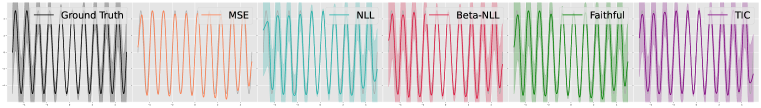
(a) Sinusoidal with $y=5.0sin(2\pi x)$ and $\sigma(x)=|x|$

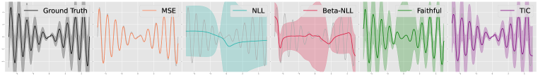
(b) Sinusoidal with $y=|x|sin(2\pi x)$ and $\sigma(x)=|x|$

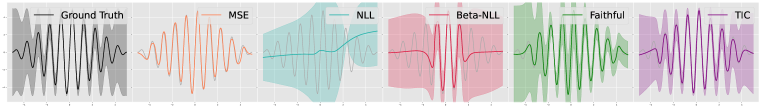
(c) Sinusoidal with $y=(5-|x|)sin(2\pi x)$ and $\sigma(x)=|x|$

Figure 4: Synthetic-Univariate. We show that the variances learnt by mapping may not explain the randomness in the model predictions. In comparison, the Taylor Induced Covariance (TIC) performs better since it explains the (co-)variance of the predictions through the model gradient and curvature.

4 TAC: Task Agnostic Correlations

How can we quantify the accuracy of our covariance estimates in the absence of ground truth annotation? Existing techniques (Kendall & Gal, 2017; Seitzer et al., 2022; Stirn et al., 2023) use metrics such as likelihood scores and mean square error for evaluation. However, these methods are skewed towards learning the mean; a perfect estimator $f_{\theta}(x)$ for the mean would result in zero mean square error, while log-likelihood scores put greater emphasis on the determinant of the covariance and does not asses correlations. Therefore, we argue for the use of a much more direct method to assess the covariance. Specifically, we reason that the goal of estimating the covariance is to encode the relation between the target variables. Therefore, partially observing a set of correlated targets should improve the prediction of the hidden targets since by definition the covariance encodes this correlation. As an example, if $P$ and $Q$ are correlated, then observing $P$ should improve our estimate of $Q$. Hence, we propose a new metric that evaluates the accuracy of correlations which we call the Task Agnostic Correlations (TAC) which is illustrated in Fig. 2.

Formally, given an $n$-dimensional target prediction $\hat{{\bm{y}}}$, ground truth ${\bm{y}}$ and the predicted covariance $\mathrm{Cov}(f_{\theta}({\bm{x}}))$, we define the Task Agnostic Correlations error as $\sum_{i}|y_{i}-\tilde{y}_{i}|/n$, where $\tilde{y}_{i}$ is the updated mean obtained after conditioning $\mathcal{N}(\tilde{y}_{i},\mathrm{Cov}(f_{\theta}({\bm{x}}))|{\bm{y}}_{j\neq i},{\bm{x}})$. For each prediction $\hat{y}_{i}$, we obtain its revised estimate $\tilde{y}_{i}$ by conditioning it over the ground truth of the remaining variables ${\bm{y}}_{i\neq j}$. We measure the absolute error of this revised estimate against the ground truth of the unobserved variable and repeat for all $i$. An accurate estimate of $\mathrm{Cov}f_{\theta}({\bm{x}})$ will decrease the error whereas an incorrect estimate will cause an increase. We highlight that this metric is agnostic of downstream tasks involving covariance estimation. Therefore, we use TAC as a metric for all multivariate experiments.

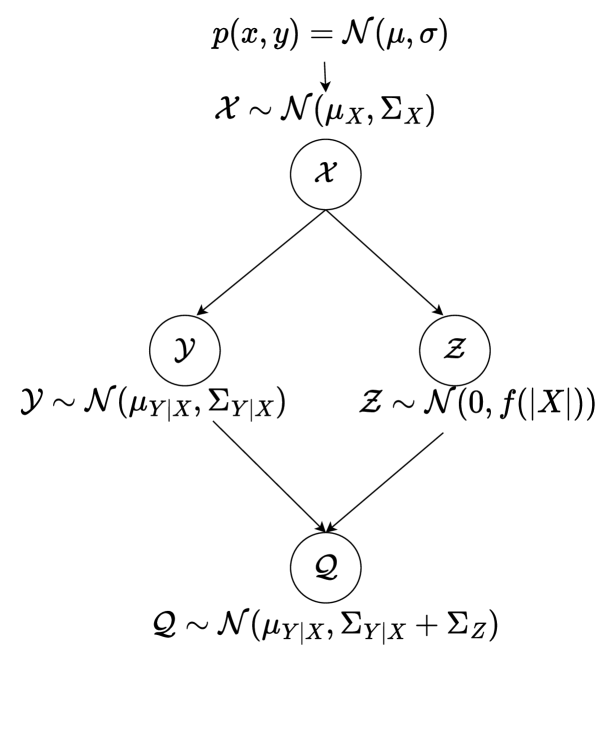
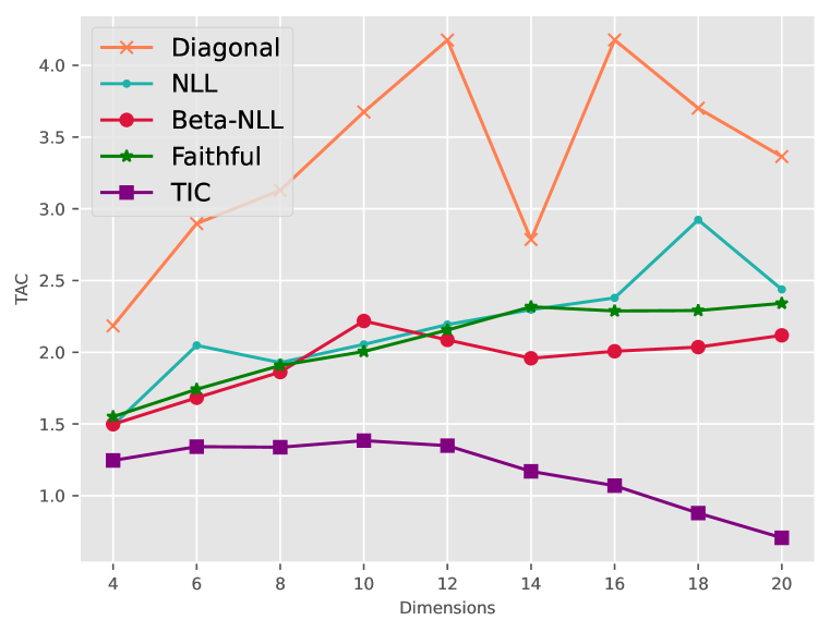
Figure 5: Synthetic-Multivariate. (Left) Experiment Design: We simulate correlated input-target variables with heteroscedastic covariance. (Right) Results: We plot the Task Agnostic Correlations (TAC) metric (y-axis) for all methods from dimensions 4 to 20 (x-axis). We show that the gap between the Taylor Induced Covariance (TIC) and other baselines widens with increasing dimensionality.

5 Experiments

The goal of this paper is towards accurate covariance estimation, and we design multiple experiments to examine our claims. Unlike previous literature, we specifically focus on multivariate outputs, which requires us to readdress several existing experimental designs for this requirement. Our experiments span across multiple datasets and network architectures, allowing for a thorough comparison of all methods. Our synthetic experiments consist of learning a univariate sinusoidal, which is inspired from Seitzer et al. (2022), as well as a novel multivariate experiment. We conduct our real-world experiments on the UCI regression repository (Dua & Graff, 2017) as well as on the MPII Andriluka et al. (2014) and LSP-LSPET (Johnson & Everingham, 2010; 2011) 2D human pose estimation datasets. Our baselines consist of the negative log-likelihood, which provides the foundation for all other methods. In addition, we compare with the diagonal covariance, which is equivalent in formulation to (Kendall & Gal, 2017), and with recent methods such as $\beta$-NLL (Seitzer et al., 2022) and Faithful Heteroscedastic Regression (Stirn et al., 2023). We take special care to provide a fair comparison; all methods are initialized with the same mean and covariance estimators. Additionally, each method has its own optimizer and learning rate scheduler. Furthermore, the batching and ordering of samples is the same for all methods.

We conduct multiple trials for each experiment and report the mean and not the standard deviation, since standard deviation is a measure of consistency and accounts for the randomness of different runs in the same evaluation setting. However in our experiments we use different settings for each run. This change includes defining new splits for input-output variables (UCI regression) as well as new multivariate distributions (synthetic multivariate) for each run. As a result some input-output splits and distributions are significantly difficult to learn and therefore distort the standard deviation. In comparison, the mean value takes into account this difficulty since if the setting is difficult for one method, it is difficult for all, and hence affects all results similarly. Therefore we avoid using standard deviation which can be distorted by difficult splits/covariance initialization and instead report the mean across multiple runs. Additionally, in the absence of annotation for the covariance, we do not make separate training and evaluation splits to increase the number of samples available for covariance estimation. While this may seem unconventional, we reason that the covariance is a measure of correlation as well as variance. If too few samples are provided for training then the resulting covariance $\mathrm{Cov}(\hat{{\bm{y}}})$ is nearly singular. Moreover, our evaluation remains fair since covariance estimation is unsupervised and our experimental methodology is the same for all approaches.

5.1 Synthetic Data

Univariate. We repeat the experiments of Seitzer et al. (2022) with a major revision. First, we introduce heteroscedasticity and substantially increase the variance of the samples. Second, we simulate different sinusoidals having constant and varying amplitudes. We draw 50,000 samples and train a fully-connected network with Batch Normalization for 100 epochs.

Our experiments show that the negative log-likelihood and $\beta$-NLL fail to converge under noisy conditions. The negative log-likelihood incorrectly overestimates the variance due to the arbitrary mapping in the absence of supervision. The gradient updates in $\beta$-NLL are susceptible to large variances, which may negatively impact optimization, as shown in Fig. 4 (c). While faithful heteroscedastic regression (FHR) uses the mean squared error objective to achieve faster convergence, the resulting variance is incorrectly estimated. We theorize that this is because FHR trains the mean estimator assuming homoscedastic unit variance, whereas the variance estimator needs to model heteroscedasticity based on the homoscedastic assumption of the mean squared error.

Multivariate. We propose an additional synthetic data experiment for multivariate analysis to study heteroscedastic covariance. We let $X,Y$ be jointly distributed and sample ${\bm{x}}$ from this distribution. Subsequently, we sample ${\bm{y}}$ conditioned on ${\bm{x}}$. To simulate heteroscedasticity, we draw samples from $Z$, a new random variable whose covariance $\Sigma_{Z}=\text{diag}(\sqrt{|{\bm{x}}|})$ depends on ${\bm{x}}$. Since $Y$ and $Z$ are independent given $X$, their sum also satisfies the normal distribution $Q|X\sim\mathcal{N}(\mu_{Y|X},\Sigma_{Y|X}+\Sigma_{Z|X})$. Therefore, the goal of this experiment is to model the mean and the heteroscedastic covariance of $Q$ conditioned on observations ${\bm{x}}$. The schematic for our experimental design is shown in Fig. 5.

For our experiments, we vary the dimensionality of ${\bm{x}}$ and ${\bm{q}}$ from 4 to 20 in steps of 2, and report the mean of ten trials for each dimension. We draw 4000 to 20000 samples depending on the dimensionality and report our results using the TAC metric. We observe two trends in Fig. 5: first, as the dimensionality of the samples increases, the gap between the Taylor Induced Covariance and other methods widens. This is because with increasing dimensionality, the number of free parameters to estimate in the covariance matrix grows quadratically. An increase in parameters typically requires a non-linear growth in the number of samples for robust fitting. As a result, the difficulty of the mapping $\mathrm{Cov}(\hat{{\bm{y}}})=g_{\Theta}({\bm{x}})$ increases with dimensionality. Second, we observe the curious trend of the decrease in the TAC metric for TIC as dimensionality increases. We believe this to be due to the fact that our ability to uniformly sample from high-dimensional spaces is limited, restricting the number of samples. Moreover, it is easier to fit few samples in high-dimensional spaces than fitting the same number of samples in low dimensions.

Table 1: UCI Regression. We compute ten trials over all the datasets and report the mean Task Agnostic Correlations (TAC) error. We show that the Taylor Induced Covariance (TIC) outperforms all baselines on ten out of twelve datasets. While TIC is not the best performing method on Naval and Parkinson, the value of TAC is small and comparable to other baselines.

Method	Abalone	Air	Appliances	Concrete	Electrical	Energy	Turbine	Naval	Parkinson	Power	Red Wine	White Wine
Diagonal	5.49	8.03	11.71	7.86	10.06	7.12	7.07	4.31	8.56	8.16	7.96	8.44
NLL	3.28	3.42	2.41	4.16	7.14	5.10	3.40	0.18	1.86	6.22	5.81	7.26
$\beta$-NLL Seitzer et al. (2022)	2.85	5.67	4.89	7.21	8.41	6.17	5.03	1.15	5.48	6.73	6.96	7.08
Faithful Stirn et al. (2023)	2.96	3.27	1.79	3.93	7.36	2.90	3.29	0.20	1.68	5.81	5.74	6.89
TIC (Ours)	1.83	2.27	1.39	2.82	4.89	2.34	2.40	0.28	2.54	3.87	4.05	4.60

5.2 UCI Regression

We perform our analysis on twelve multivariate UCI regression (Dua & Graff, 2017) datasets which have been used in previous work on negative log-likelihood Stirn et al. (2023); Seitzer et al. (2022). We select datasets where a majority of the features are continuous valued. Since the goal of this work is to study covariance estimation, we use different pre-processing since many of the datasets have univariate or low-dimensional targets. For each dataset we randomly allocate 25% of the features as input and the remaining 75% features as multivariate targets at run-time. Indeed, some combinations of input variables may fare poorly at predicting the target variables. However, this is an interesting challenge for the covariance estimator, which needs to learn the underlying correlations even in unfavourable circumstances. Moreover, random splitting also allows our experiments to remain unbiased since we do not control the split of variables at all.

For all datasets, we follow the established machine learning practice of normalizing our datasets. Normalizing also allows us to directly compare the TAC metric across various datasets. We perform 10 trials for each dataset and report our results in Table 1. We show that TIC outperforms all baselines on ten out of twelve datasets. We note that the TAC metric is small across all methods for the remaining two datasets.

5.3 2D Human Pose Estimation

We introduce experiments on human pose  (Kreiss et al., 2019; 2021; Newell et al., 2016; Liu & Ferrari, 2017; Shukla & Ahmed, 2021; Shukla, 2022; Yoo & Kweon, 2019; Shukla et al., 2022; Gong et al., 2022) particularly because of the challenges it poses to modeling TIC. Popular human pose architectures such as the hourglass (Newell et al., 2016) are fully convolutional, whereas all our previous experiments have focused on fully-connected architectures. Additionally, while TIC assumes ${\bm{x}}\in\mathbb{R}^{m}$ and ${\bm{y}}\in\mathbb{R}^{n}$, human pose estimation relies on input images ${\bm{\mathsfit{X}}}\in\mathbb{R}^{C\times H\times W}$ and output heatmaps ${\bm{\mathsfit{Y}}}\in\mathbb{R}^{\#\text{joints}\times 64\times 64}$. However, we show that TIC outperforms all baselines on human pose with just a few modifications. The first modification is the use of soft-argmax (Li et al., 2021b; a), which reduces the output heatmap to a keypoint vector ${\bm{y}}\in\mathbb{R}^{\text{\#joints}*2}$. The second modification recursively calls the hourglass module till we obtain a one-dimensional vector encoding which serves as the input for our method.

We use the popular Stacked Hourglass (Newell et al., 2016) as our backbone for human pose estimation. We run our experiments on two popular single person datasets: MPII (Andriluka et al., 2014) and Leeds Sports Pose (LSP-LSPET) (Johnson & Everingham, 2010; 2011). We perform our analysis by merging the MPII and LSP-LSPET datasets to increase the number of samples. We continue to use TAC as our metric since for single person estimation, the scale of the person is fixed and hence TAC is highly correlated to PCKh/PCK (the preferred metric for multi-person multi-scale pose estimation). Moreover, the Euclidean distance as a measure of error is also used in MPJPE, which is another well-known evaluation metric for human pose. We perform five trials and report our results in Table 2. Our experiments show that the TIC outperforms all baselines and is successfully able to scale to convolutional architectures.

Table 2: 2D Human Pose Estimation. We compare the Taylor Induced Covariance (TIC) using the Task Agnostic Correlations (TAC) metric with other methods on the combined MPII and LSP/LSPET datasets. We show that TIC can scale to convolutional architectures and outperform baselines across all joints.

Method	head	neck	lsho	lelb	lwri	rsho	relb	rwri	lhip	lknee	lankl	rhip	rknee	rankl	Avg
MSE	5.53	7.88	7.31	8.73	10.52	7.01	8.41	10.19	8.43	8.53	10.53	8.13	8.37	10.58	8.58
Diagonal	5.36	7.23	6.95	8.17	10.01	6.48	7.79	9.73	8.11	8.30	11.12	7.75	8.17	11.20	8.32
NLL	4.48	6.81	5.38	5.19	7.13	5.11	4.86	6.89	6.62	6.35	8.45	6.43	6.17	8.40	6.31
$\beta$-NLL Seitzer et al. (2022)	4.63	7.14	6.74	8.23	9.98	6.43	7.92	9.65	8.01	8.13	10.12	7.71	7.93	10.19	8.06
Faithful Stirn et al. (2023)	5.13	6.36	5.32	4.94	7.18	4.96	4.72	6.85	6.67	6.29	8.39	6.36	6.22	8.37	6.27
TIC (Ours)	3.76	5.98	4.80	4.64	6.34	4.46	4.41	6.12	6.09	5.82	7.59	5.79	5.63	7.55	5.64

6 Limitations

The Taylor Induced Covariance is computationally expensive since the local curvature needs to be computed for each sample. While GPU parallelization through vmap helps alleviate the problem, the method is not real-time. However, our method shares this challenge with optimization research, and we believe that advances in optimization including fast and accurate approximations of the curvature with respect to the input sample would directly benefit our method.

7 Conclusion

This paper studied unsupervised heteroscedastic covariance estimation through parametric neural networks. We addressed a key limitation in negative log-likelihood; in the absence of supervision, $\mathrm{Cov}(\hat{{\bm{y}}})=g_{\Theta}({\bm{x}})$ is essentially an arbitrary mapping of ${\bm{x}}$ to a positive definite matrix which may not represent the randomness in $\hat{{\bm{y}}}$. Our solution, the Taylor Induced Covariance (TIC), is a novel derivation of a closed-form expression for $\mathrm{Cov}(\hat{{\bm{y}}})$ through its Taylor polynomial. Doing so allowed us to represent the variation in $\hat{y}$ through its gradient and curvature. Additionally, we addressed the lack of direct methods to evaluate the covariance by proposing the Task Agnostic Correlations (TAC) metric. The metric uses conditioning of the normal distribution to quantify the accuracy of learnt correlations. We performed extensive experiments using the TIC-TAC framework across multiple datasets and network architectures. Our results show that TIC outperforms all baselines and thereby motivating the use of the TIC-TAC framework for covariance estimation.

References

- Andriluka et al. (2014) Mykhaylo Andriluka, Leonid Pishchulin, Peter Gehler, and Bernt Schiele. 2d human pose estimation: New benchmark and state of the art analysis. In IEEE Conference on Computer Vision and Pattern Recognition (CVPR), June 2014.
- Barratt & Boyd (2022) Shane Barratt and Stephen Boyd. Covariance prediction via convex optimization. Optimization and Engineering, pp. 1–34, 2022.
- Biswas et al. (2020) Sourav Biswas, Yihe Dong, Gautam Kamath, and Jonathan Ullman. Coinpress: Practical private mean and covariance estimation. In H. Larochelle, M. Ranzato, R. Hadsell, M.F. Balcan, and H. Lin (eds.), Advances in Neural Information Processing Systems, volume 33, pp. 14475–14485. Curran Associates, Inc., 2020. URL https://proceedings.neurips.cc/paper_files/paper/2020/file/a684eceee76fc522773286a895bc8436-Paper.pdf.
- Chen et al. (2017) Xixian Chen, Michael R. Lyu, and Irwin King. Toward efficient and accurate covariance matrix estimation on compressed data. In Doina Precup and Yee Whye Teh (eds.), Proceedings of the 34th International Conference on Machine Learning, volume 70 of Proceedings of Machine Learning Research, pp. 767–776. PMLR, 06–11 Aug 2017. URL https://proceedings.mlr.press/v70/chen17g.html.
- Dorta et al. (2018) Garoe Dorta, Sara Vicente, Lourdes Agapito, Neill DF Campbell, and Ivor Simpson. Structured uncertainty prediction networks. In Proceedings of the IEEE conference on computer vision and pattern recognition, pp. 5477–5485, 2018.
- Dua & Graff (2017) Dheeru Dua and Casey Graff. UCI machine learning repository, 2017. URL http://archive.ics.uci.edu/ml.
- Gilmer et al. (2022) Justin Gilmer, Behrooz Ghorbani, Ankush Garg, Sneha Kudugunta, Behnam Neyshabur, David Cardoze, George Edward Dahl, Zachary Nado, and Orhan Firat. A loss curvature perspective on training instabilities of deep learning models. In International Conference on Learning Representations, 2022. URL https://openreview.net/forum?id=OcKMT-36vUs.
- Gong et al. (2022) Jia Gong, Zhipeng Fan, Qiuhong Ke, Hossein Rahmani, and Jun Liu. Meta agent teaming active learning for pose estimation. In Proceedings of the IEEE/CVF Conference on Computer Vision and Pattern Recognition, pp. 11079–11089, 2022.
- Gu et al. (2021) Min-Hee Gu, Chihyun Cho, Hahng-Yun Chu, No-Weon Kang, and Joo-Gwang Lee. Uncertainty propagation on a nonlinear measurement model based on taylor expansion. Measurement and Control, 54(3-4):209–215, 2021.
- Gundavarapu et al. (2019) Nitesh B Gundavarapu, Divyansh Srivastava, Rahul Mitra, Abhishek Sharma, and Arjun Jain. Structured aleatoric uncertainty in human pose estimation. In CVPR Workshops, volume 2, 2019.
- Hoff et al. (2022) Peter Hoff, Andrew McCormack, and Anru R Zhang. Core shrinkage covariance estimation for matrix-variate data. arXiv preprint arXiv:2207.12484, 2022.
- ISO & OIML (1995–2020) I ISO and BIPM OIML. Guide to the expression of uncertainty in measurement. Geneva, Switzerland, 122:16–17, 1995–2020.
- Jacot et al. (2018) Arthur Jacot, Franck Gabriel, and Clément Hongler. Neural tangent kernel: Convergence and generalization in neural networks. Advances in neural information processing systems, 31, 2018.
- Johnson & Everingham (2010) Sam Johnson and Mark Everingham. Clustered pose and nonlinear appearance models for human pose estimation. In Proceedings of the British Machine Vision Conference, 2010. doi:10.5244/C.24.12.
- Johnson & Everingham (2011) Sam Johnson and Mark Everingham. Learning effective human pose estimation from inaccurate annotation. In Proceedings of IEEE Conference on Computer Vision and Pattern Recognition, 2011.
- Kanazawa & Kanatani (2003) Yasushi Kanazawa and Kenichi Kanatani. Do we really have to consider covariance matrices for image feature points? Electronics and communications in Japan (part III: Fundamental electronic science), 86(1):1–10, 2003.
- Kastner (2019) Gregor Kastner. Sparse bayesian time-varying covariance estimation in many dimensions. Journal of Econometrics, 210(1):98–115, 2019.
- Kendall & Gal (2017) Alex Kendall and Yarin Gal. What uncertainties do we need in bayesian deep learning for computer vision? In Advances in neural information processing systems, pp. 5574–5584, 2017.
- Kingma & Ba (2015) Diederik P Kingma and Jimmy Ba. Adam: a method for stochastic optimization. In International Conference on Learning Representations, 2015.
- Kirkup & Frenkel (2006) Les Kirkup and Robert B Frenkel. An introduction to uncertainty in measurement: using the GUM (guide to the expression of uncertainty in measurement). Cambridge University Press, 2006.
- Kreiss et al. (2019) Sven Kreiss, Lorenzo Bertoni, and Alexandre Alahi. Pifpaf: Composite fields for human pose estimation. In Proceedings of the IEEE/CVF conference on computer vision and pattern recognition, pp. 11977–11986, 2019.
- Kreiss et al. (2021) Sven Kreiss, Lorenzo Bertoni, and Alexandre Alahi. Openpifpaf: Composite fields for semantic keypoint detection and spatio-temporal association. IEEE Transactions on Intelligent Transportation Systems, 23(8):13498–13511, 2021.
- Lakshminarayanan et al. (2017) Balaji Lakshminarayanan, Alexander Pritzel, and Charles Blundell. Simple and scalable predictive uncertainty estimation using deep ensembles. Advances in neural information processing systems, 30, 2017.
- Le et al. (2005) Quoc V Le, Alex J Smola, and Stéphane Canu. Heteroscedastic gaussian process regression. In Proceedings of the 22nd international conference on Machine learning, pp. 489–496, 2005.
- Li et al. (2021a) Jiefeng Li, Tong Chen, Ruiqi Shi, Yujing Lou, Yong-Lu Li, and Cewu Lu. Localization with sampling-argmax. Advances in Neural Information Processing Systems, 34:27236–27248, 2021a.
- Li et al. (2021b) Jiefeng Li, Chao Xu, Zhicun Chen, Siyuan Bian, Lixin Yang, and Cewu Lu. Hybrik: A hybrid analytical-neural inverse kinematics solution for 3d human pose and shape estimation. In Proceedings of the IEEE/CVF conference on computer vision and pattern recognition, pp. 3383–3393, 2021b.
- Liu & Ferrari (2017) Buyu Liu and Vittorio Ferrari. Active learning for human pose estimation. In Proceedings of the IEEE International Conference on Computer Vision, pp. 4363–4372, 2017.
- Liu et al. (2018) Katherine Liu, Kyel Ok, William Vega-Brown, and Nicholas Roy. Deep inference for covariance estimation: Learning gaussian noise models for state estimation. In 2018 IEEE International Conference on Robotics and Automation (ICRA), pp. 1436–1443, 2018. doi: 10.1109/ICRA.2018.8461047.
- Lu & Koniusz (2022) Changsheng Lu and Piotr Koniusz. Few-shot keypoint detection with uncertainty learning for unseen species. In Proceedings of the IEEE/CVF Conference on Computer Vision and Pattern Recognition, pp. 19416–19426, 2022.
- Ly et al. (2017) Alexander Ly, Maarten Marsman, Josine Verhagen, Raoul PPP Grasman, and Eric-Jan Wagenmakers. A tutorial on fisher information. Journal of Mathematical Psychology, 80:40–55, 2017.
- Newell et al. (2016) Alejandro Newell, Kaiyu Yang, and Jia Deng. Stacked hourglass networks for human pose estimation. In Bastian Leibe, Jiri Matas, Nicu Sebe, and Max Welling (eds.), Computer Vision – ECCV 2016, pp. 483–499, Cham, 2016. Springer International Publishing. ISBN 978-3-319-46484-8.
- Nguyen et al. (2022) Viet Anh Nguyen, Daniel Kuhn, and Peyman Mohajerin Esfahani. Distributionally robust inverse covariance estimation: The wasserstein shrinkage estimator. Operations research, 70(1):490–515, 2022.
- Petersen & Pedersen (2012) K. B. Petersen and M. S. Pedersen. The matrix cookbook, nov 2012. URL http://www2.compute.dtu.dk/pubdb/pubs/3274-full.html. Version 20121115.
- Russell & Reale (2021) Rebecca L Russell and Christopher Reale. Multivariate uncertainty in deep learning. IEEE Transactions on Neural Networks and Learning Systems, 33(12):7937–7943, 2021.
- Seitzer et al. (2022) Maximilian Seitzer, Arash Tavakoli, Dimitrije Antic, and Georg Martius. On the pitfalls of heteroscedastic uncertainty estimation with probabilistic neural networks. In International Conference on Learning Representations, 2022. URL https://openreview.net/forum?id=aPOpXlnV1T.
- Shukla (2022) Megh Shukla. Bayesian uncertainty and expected gradient length-regression: Two sides of the same coin? In Proceedings of the IEEE/CVF Winter Conference on Applications of Computer Vision, pp. 2367–2376, 2022.
- Shukla & Ahmed (2021) Megh Shukla and Shuaib Ahmed. A mathematical analysis of learning loss for active learning in regression. In Proceedings of the IEEE/CVF Conference on Computer Vision and Pattern Recognition (CVPR) Workshops, pp. 3320–3328, June 2021.
- Shukla et al. (2022) Megh Shukla, Roshan Roy, Pankaj Singh, Shuaib Ahmed, and Alexandre Alahi. Vl4pose: Active learning through out-of-distribution detection for pose estimation. In Proceedings of the 33rd British Machine Vision Conference, number CONF. BMVA Press, 2022.
- Shynk (2012) John J Shynk. Probability, random variables, and random processes: theory and signal processing applications. John Wiley & Sons, 2012.
- Simpson et al. (2022) Ivor JA Simpson, Sara Vicente, and Neill DF Campbell. Learning structured gaussians to approximate deep ensembles. In Proceedings of the IEEE/CVF Conference on Computer Vision and Pattern Recognition, pp. 366–374, 2022.
- Stirn et al. (2023) Andrew Stirn, Harm Wessels, Megan Schertzer, Laura Pereira, Neville Sanjana, and David Knowles. Faithful heteroscedastic regression with neural networks. In International Conference on Artificial Intelligence and Statistics, pp. 5593–5613. PMLR, 2023.
- Tirado-Garín et al. (2023) Javier Tirado-Garín, Frederik Warburg, and Javier Civera. Dac: Detector-agnostic spatial covariances for deep local features. arXiv preprint arXiv:2305.12250, 2023.
- Van Amersfoort et al. (2020) Joost Van Amersfoort, Lewis Smith, Yee Whye Teh, and Yarin Gal. Uncertainty estimation using a single deep deterministic neural network. In International Conference on Machine Learning, pp. 9690–9700. PMLR, 2020.
- Yoo & Kweon (2019) D. Yoo and I. S. Kweon. Learning loss for active learning. In 2019 IEEE/CVF Conference on Computer Vision and Pattern Recognition (CVPR), pp. 93–102, 2019. doi: 10.1109/CVPR.2019.00018.