Probabilistic Feature Augmentation for AIS-Based Multi-Path Long-Term Vessel Trajectory Forecasting

Abstract

Maritime transportation is paramount in achieving global economic growth, entailing concurrent ecological obligations in sustainability and safeguarding endangered marine species, most notably preserving large whale populations. In this regard, the Automatic Identification System (AIS) data plays a significant role by offering real-time streaming data on vessel movement, allowing enhanced traffic monitoring. AIS data have improved maritime safety by reducing vessel-to-vessel collisions, but this study delves into utilizing AIS data as a proactive measure for averting vessel-to-whale ones. This paper tackles an intrinsic problem to trajectory forecasting: the effective multi-path long-term vessel trajectory forecasting on engineered sequences of AIS data. For such a task, we have developed an encoder-decoder model architecture using Bidirectional Long Short-Term Memory Networks (Bi-LSTM) to predict the next 12 hours of vessel trajectories using 1 to 3 hours of AIS data as input. We feed the model with probabilistic features engineered from historical AIS data that refer to each trajectory’s potential route and destination. The model then predicts the vessel’s trajectory, considering these additional features by leveraging convolutional layers for spatial feature learning and a position-aware attention mechanism that increases the importance of recent timesteps of a sequence during temporal feature learning. The probabilistic features have an F1 Score of approximately 85% and 75% for each feature type, respectively, demonstrating their effectiveness in augmenting information to the neural network. We test our model on the Gulf of St. Lawrence, a region known to be the habitat of North Atlantic Right Whales (NARW). Our model achieved a $R^{2}$ score of over 98% in different techniques using varying features. The high $R^{2}$ score is a natural outcome of the well-defined shipping lanes. However, our model stands out among other forecasting approaches as it demonstrates the capability of complex decision-making during turnings and path selection. Also, we have shown that our model can achieve more accurate forecasting with average and median forecasting errors of 11km and 6km, respectively. Overall, our study demonstrates the potential of data engineering and trajectory forecasting models for marine life species preservation.

Introduction

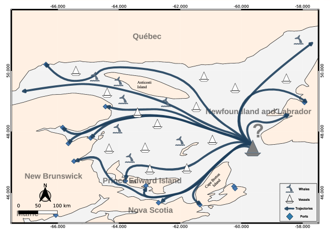
Figure 1: Potential routes a vessel may take to enter the Gulf of St. Lawrence through the Cabot Strait. Whale and vessel symbols represent high vessel traffic in the region and the possibility of marine life encounters along the possible routes. Possible destinations include Quebec, New Brunswick, Nova Scotia, Newfoundland and Labrador ports. A vessel can anchor in one of these ports, continue into the St. Lawrence River, or exit the gulf through the Strait of Belle Isle. The figure illustrates that vessels can have a common start point but may take different routes, resulting in different trajectories.

Maritime transportation plays a vital role in global economic development but shares the aim of becoming environmentally sustainable. The International Maritime Organization (IMO) was established to encourage and implement policies related to maritime safety, navigation efficiency, and the prevention of marine pollution by ships [1]. Its primary function is to improve traffic surveillance and vessel safety by providing real-time information about vessel movement [2]. The Automatic Identification System (AIS) is a technology used to track the location of marine vessels worldwide, and according to Canadian regulations (Section 65 of the Navigation Safety Regulations), every Canadian or foreign vessel heading to Canada is required to have an AIS transceiver that can provide information about its route and receive information about nearby vessels. By using terrestrial and satellite receivers to capture transmissions, vessels can be tracked, improving our awareness about vessel movement in the ocean. This technology is beneficial not only for individual vessel tracking but also for shore-based facilities like the Coast Guard’s Marine communications and traffic services, which can remotely monitor collective traffic and individual movements, acting to prevent distress situations [3, 4, 5], such as collisions along the route (see Figure 1).

AIS messages are transmitted in an encoded format, and among the content transmitted, the most common and relevant to this paper are the vessel coordinates (Longitude and Latitude); besides those, an AIS message also provides Speed over Ground (SOG), Course over Ground (COG), timestamps, identification information (e.g., Maritime Mobile Service Identity — MMSI and/or IMO identifiers) and vessel dimensions (e.g., width and height) within its content. These messages are transmitted by most vessels every 2–10 seconds or 3–5 minutes, depending on the status, qualifications, and purposes of the vessel [6, 7]. The vast amount of data broadcasted worldwide, with approximately 500–600 million messages per day [8], has become the source of constructing AIS datasets. These datasets contain spatial-temporal data and have been widely exploited for applications that require the analysis of mobility patterns and management of shipping routes [9, 10, 8, 11, 12]. Handling AIS data can be complex because of the large amount of data involved, which contains messages that are damaged, duplicated, or otherwise incorrect [13, 14, 15].

The challenge of obtaining high-quality data is further impaired by the limited availability of freely accessible datasets. Open-source datasets often fail to meet the quality standards of paid or government-classified data sources, adding to the difficulty of cleaning, segmenting, and interpolating the data. Researchers in the scientific community have been struggling to develop efficient techniques and pipelines to address these issues and eliminate noise from the data [16, 17, 18]. However, this remains an open challenge as most techniques are tailored to specific research projects and are not publicly available.

Research on AIS datasets has opened the doors to enhance maritime safety and security through solving various issues such as the detection of suspicious events [19], monitoring traffic to avoid collisions [12, 20], and evaluating noise or environmental pollution levels [21, 22]. Recently, the problem of forecasting long-term trajectories [23, 24, 25, 26] of vessels gained significant attention to reduce vessel accidents, detect anomalous trajectories, and improve path planning — especially for autonomous shipping [27, 28, 29, 30, 31, 32, 33]. The study of trajectory forecasting has a diverse background, where different techniques have been employed to create models that predict movement, either from vessels or different vehicles. One of the most basic models is the constant velocity model [34], derived from the AIS messages’ geographical coordinates and the vessel’s SOG and COG at the last recorded timestep, assuming no change in speed and course for the forecasting duration. More refined models go beyond these assumptions and use the trajectory’s geometry to produce more accurate predictions, such as the Ornstein–Uhlenbeck process adapted to vessel trajectory forecasting [35]. Machine learning and deep learning have advanced significantly in recent years, allowing for the creation of complex models that combine different types of data. However, the real-world use of these models is often limited due to the difficulty of synchronizing and preparing diverse data in streaming conditions. To address this, research has been focusing on minimizing required features in data. In this sense, our trajectory forecasting model relies mainly on geographical coordinates, which define the trajectory geometry and can be used to calculate secondary features such as the average speed and bearing of vessels.

In a recent study by Nguyen et al. (2024) [36], authors proposed an approach to represent four AIS-related features into embeddings, i.e., a learned numerical representation of data where similar data points have a similar representation based on their meaning. Their study adopted the transformer encoder in a generative-driven approach to forecasting long-term trajectories, such as in Nguyen et al. (2021) [37]. However, their technique confines the ship’s trajectory to the centroid of the grid cells, requiring longer training sessions on a large model so it can learn the many patterns that distinguish each grid cell. This approach may be effective when ships adhere to nearly constant velocity models, but its potential to learn more individual moving patterns is overlooked. Besides this, the authors implemented their solution using teacher forcing [38], and instead of inputting the previous step predictions as input to the next step, the technique trains the network with ground truth data as that information is known during the training phase. During testing, the network is rewired to revert the need for ground truth data, expecting that the learned weights during forced training will perform better in the testing phase. To be more specific, the authors forecast information about the speed and course of the vessel, which can instead be mathematically calculated when having information about consecutive coordinates. Therefore, unless the model always provides a perfect estimation of the vessel’s speed and course, the information forwarded ahead in the model for predicting the next step of the sequence tends to be imprecise (i.e., uncertain).

In different studies, Capobianco et al. (2021) [39] and Capobianco et al. (2022) [40] have reviewed the effectiveness of recurrent encoder-decoder neural networks in trajectory forecasting. In both studies, the authors utilized comparable network architectures that employ an encoder to produce an embedding; this embedding is then utilized in an attention mechanism to allow for multi-step forecasting and take advantage of both short and long-term dependencies learning; and, the network decoder decodes the embedding and yields the forecasted trajectory. However, the issue in their modeling approach is not related to the auto-encoder model but rather to how the attention mechanism is employed. When attention is used over a sentence as seen in Large Language Models (LLMs) such as ChatGPT or Bert, the mechanism learns the significance (or importance) of words in the sentence, helping the model to focus on the key points of the sentence and respond accordingly to the LLM operator. However, sequences of AIS messages and sentences (i.e., sequences of words) have intrinsically different abstractions. In an AIS forecasting model, the knowledge that can be leveraged from the beginning of the sequence is considerably less important than the knowledge that can be extracted from later points in the same sequence because of the temporal and sequential nature of the data. This way, while the intermediate points of the sequence can aid in more accurate long-term trajectory forecasting, they also increase the uncertainty of the modeling problem in the short term because the model does not follow the correct order of events in the sequence.

Using a different approach, this paper advances previous works by using an equal-size hexagon grid for extracting probabilistic features that aid in identifying the vessel route and destination. These features allow for a finer approximation of the vessel path without being constrained by the centroids of the cells. This means that differently from Nguyen et al. (2024) [36], we tackle this problem in a regression rather than a classification fashion, where the ocean grid is a step to achieve the trajectory instead of being an anchor for the trajectories themselves. Through this approach, we developed a model that can predict 12 hours of AIS data based on 3 hours of input data, where one AIS message is sent every 10 minutes. The study focuses on the Gulf of St. Lawrence in Canada, where vessels can take different routes to reach various regional ports. The ending point (destination) of each track is known, and the purpose is to identify the paths that cargo and tanker vessels will take in an area with many possible destinations (see Figure 1).

To this end, we propose a spatio-temporal model with an encoder-decoder structure where the encoder has three stacked blocks of convolutional layers attached to a Bidirectional Long Short-Term Memory Network (Bi-LSTM). Each block has a pair of $1\mathbf{D}$ convolutions where one extracts short-and the other longer-term dependencies from the input features. Before moving forward with the Bi-LSTM decoding, our model includes a positional-aware attention mechanism, which differs from Capobianco et al. (2021) [39] and Capobianco et al. (2022) [40] by allowing the auto-encoder model to learn from all AIS points in the trajectory but consistently giving more importance to the latter timestep of the input data sequence. The proposed modeling approach uses the attention mechanism as focal attention to the more recent AIS message for a smoother transition between inputs and outputs without requiring overly complex models.

To ensure the reproducibility of our work and cope with the challenge of dealing with erroneous and noisy messages from AIS data, we have developed a sophisticated AIS data analysis tool called the Automatic Identification System Database (AISdb). Such a tool has been perfected over several years and is intended to foster research on AIS data-related fields by the scientific community. AISdb is an open-source platform that offers various tools for collecting and processing real-time and historical AIS data. It is highly flexible and compatible with live streaming and historical raw (i.e., binary encoded) AIS data files. Its interface supports various operations, including creating databases, spatio-temporal querying, processing, visualizing, and exporting curated data. AISdb includes features that enable users to seamlessly integrate AIS data with environmental data stored in raster file formats. This enables users to merge multiple environmental data sources with AIS data, enhancing the analysis and interpretation of vessel movements and their interactions with the marine environment (see Methods for more details).

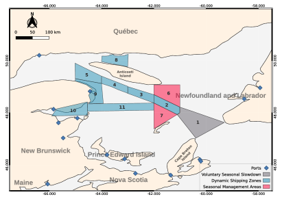
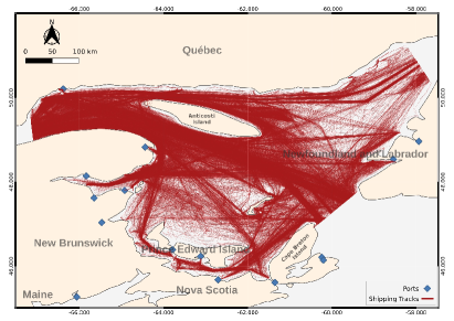
Figure 2: This study centers on the Gulf of St. Lawrence, with traffic policy zones defined by Transport Canada. These zones include voluntary seasonal slowdowns, dynamic shipping zones, and seasonal management areas and are illustrated on the left-hand map. The regulated areas overlay main vessel traffic routes, such as the main shipping corridor between the Cabot Strait (between Cape Breton Island and Newfoundland) and the estuary of the St. Lawrence River routes (polygons 1–5). These areas cover the ports in the zone between New Brunswick and Québec (polygons 6–12) and the Jacques Cartier Strait between Anticosti Island and Northern Quebec (polygon 8). The visualization on the right-hand side displays vessel tracks (2015–2020) in the area, revealing inconsistent paths within shipping lanes.

As for the evaluation, we conducted an extensive set of experiments to test various scenarios and determine the effectiveness of our proposal. We employed different sets of features and applied trigonometric transformations to them, using the results to train models with varying complexities. In such a case, we observed that the effectiveness in providing probabilistic information to the neural network is in the order of 85% and 75% of the F1 Score in predicting the route and the destination of the vessels, respectively. Those results represent the degree of certainty of the probabilistic features. Furthermore, our findings indicate that when using only coordinates, speed, course information, and their deltas (see Methods) to predict long-term trajectories, the model’s ability to make path decisions is limited for cargo and tanker vessels. This is due to the model’s tendency to perform well on straight paths but struggle on complex and curved paths, resulting in mean and median errors of 13 km and 8 km, respectively, on the test dataset shared between both vessel types. Incorporating the proposed probabilistic features resulted in mean and median errors of 12 km and 8 km, respectively. However, after applying cartesian and other trigonometrical transformations to all sets of features, the errors were reduced further, resulting in mean and median errors of 11 km and 6 km. By using the trigonometrical transformations on the probabilistic features, we were able to achieve an $R^{2}$ score higher than 98% for cargo and tankers using the proposed model, a notably high value that is due to the over occurrence of nearly straight paths in the dataset; even so, we demonstrate that our model stands out in decision-making in the face of curvy patterns and sudden route changes. Our contributions set a new milestone for long-term vessel trajectory forecasting using spatio-temporal data, probabilistic modeling of features, and advanced neural network techniques. These results have the potential to move forward with policies that can increase our awareness of the ocean, proactively aiding in reducing unintentional harm to endangered marine species, such as NARW.

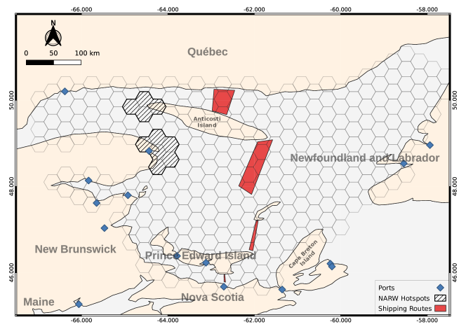
Figure 3: Gulf of St. Lawrence overlain with our hexagonal study grid. Hatched grid cells indicate hotspots for North Atlantic Right Whales [41]. Most vessels’ trajectories intersect with the red route polygons at some point during their journey through the gulf. These polygons segment the gulf from north to south, covering major inbound and outbound movements inside the gulf. However, it is important to note that not all paths are required to cross a route polygon. Vessels whose paths cross the route polygons are generally easier to forecast, while those that do not pose more intricate forecasting scenarios.

Problem Formulation

This research is motivated by the increased number of vessel-whale collisions in the Gulf of St. Lawrence (see Figure 7A), especially since 2017, when at least 12 fatalities of endangered North Atlantic Right Whales (NARW) were recorded [42], indicating that human activity such as fishing and transportation pose a significant risk to the NARW population. Developing effective strategies for managing vessel movement (see Figure 7B) and reducing the likelihood of collisions is essential to mitigate this risk. One promising approach in the face of the unpredictability of whales’ movements is to predict the vessel trajectory instead, which relies on advanced predictive models and real-time data to anticipate vessel paths that come across collision hotspot areas (see Figure 3A). As vessels navigate, their historical data provide us with insights into their likely trajectory besides observations on collective vessel movement patterns [20]; the same can be observed among people commuting [43, 44, 45], patient trajectories in hospitals [46, 47], and spatio-temporal disease-spreading phenomena [48, 49]. Accurately predicting the movement of vessels can provide valuable insights for authorities by integrating the forecasting with the movement of whales to avoid the risk of strike. This information can then be used to proactively adjust shipping routes and enforce speed restrictions in these areas, mitigating the risk of collisions and preserving the safety of marine life.

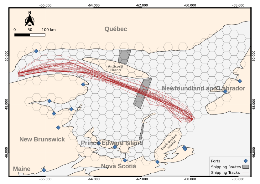
(a) Path 1

(b) Path 2

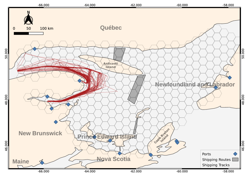
(c) Path 3

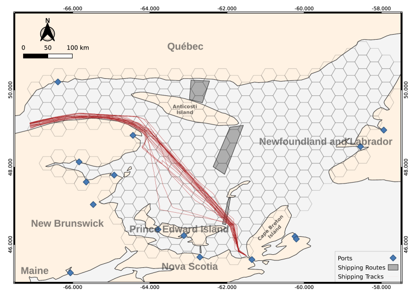
(d) Path 4

Figure 4: The Gulf of St. Lawrence region has multiple paths with high vessel traffic. This figure shows four of them, which do not represent our dataset’s complete set of trajectories but cover three major ones (1, 2, and 4) that cross a route polygon. Path 3, on the other hand, does not intersect with any route polygon. Instead, it represents tracks that interact with all major hotspots of NARW in the gulf.

The challenge we are addressing involves more than just the forecasting trajectories under the unpredictability of whales’ locations. In the Gulf of St. Lawrence, ships can take various paths, even if their start and end are known beforehand (see Figure 3). This difficulty comes from the fact that no physical grid directs ships into specific lanes, unlike city streets [50, 51, 52]. Although traffic management policies designate shipping lanes, the lanes do not restrict the movement of vessels as they may enter or exit lanes at different points throughout the gulf. As a result, predicting ship trajectories becomes challenging, especially for longer distances, as the predicted paths deviate significantly from actual paths with increased elapsed time and travel distance. Therefore, we require a deep-learning model to learn from the input AIS data and its routing possibilities to understand the relationship between mobility constraints and moving patterns.

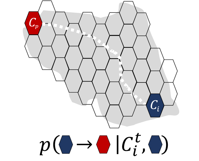
(a) Traditional Formulation

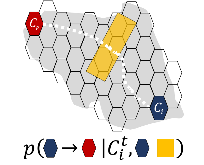
(b) Proposed Formulation

Figure 5: Probabilistic formulations of long-term trajectory forecasting. In the traditional method (a), the probabilistic matrix is utilized to determine the most likely whereabouts of a vessel by analyzing its movements concerning its starting point ($C_{i}$) on a grid using historical data. Our proposed approach (b) follows a similar method but with new features and a revisited understanding. In addition to historical data, the potential route depends on traversing the polygons. Essentially, our model employs route polygons as a type of memory to provide more precise guidance on the vessel’s decisions at different moments in the past, aiming for a more reliable and effective probabilistic-based inference system.

To solve this problem, we first split the gulf into hexagonal grid cells (see Figure 3) of $0.3^{\mathrm{o}}$ on EPSG:4269 projection. The shape of the cells is due to the Earth’s curvature, as hexagonal cells can divide the Earth’s surface uniformly. Figure 4 shows some paths discovered from historical data, highlighted by polygons placed in high-traffic areas. The intuition for utilizing grid cells is extracting the starting and destination area of tracks because the AIS data does not always provide detailed information regarding the destination of a voyage. Relationships between grid cells based on tracks will assist the decision-making of the AI model while forecasting trajectory in the absence of information related to the destination. In addition, there are countless possible locations for vessels in the gulf, making it difficult to compare them with others that have different, but yet similar, trajectories. Using grid cells helps us to overcome these challenges and allows for a more effective comparison between vessels that pass through the same grid cell. In this sense, comparing trajectories and the route polygons we placed in high-traffic areas, we can see that most tracks intersect with route polygons at some point during their course. However, paths like the one in Figure 4C are the most challenging ones in the dataset as it does not intersect with any route polygons and represent a curvy-shaped moving pattern. We developed a probabilistic model (see Algorithm 1) that leverages the relationship between grid cells, route polygons, and historical vessel tracks to predict the route a vessel will take and the destination (i.e., last grid cell) of the voyage. For the sake of disambiguation, this research proposes two models, one for engineering features and referred to as the probabilistic model, and another to forecast the trajectories, referred to as the deep-learning model.

Understanding the historical movements and patterns of vessels is essential in this approach. Our probabilistic model, as shown in Figure 5B, considers the relationship of tracks with route polygons and grid cells that highlight major paths in the gulf. By calculating the (1) number of tracks going to a particular destination (a grid cell), (2) the direction of each track at the point where it intersects with a route polygon, and (3) the probability score of each surrounding cell as a potential destination for each track, we can gain valuable insights into ship behavior and the routes they take. The primary objective of this approach (i.e., probabilistic model) is to predict the probable destination (grid cell) while considering the vessel’s current position. This is achieved by computing the difference, through the Euclidean distance, between the motion behavior of the vessel in the grid cell where it lies and the historical motion behavior of vessels in each possible destination. We consider grid information and AIS messages to determine probability scores and potential destinations for a vessel. The output of this process is a set of engineered features that indicate the route and destination of a vessel for the problem of long-term multi-path trajectory forecasting.

Pipeline Overview

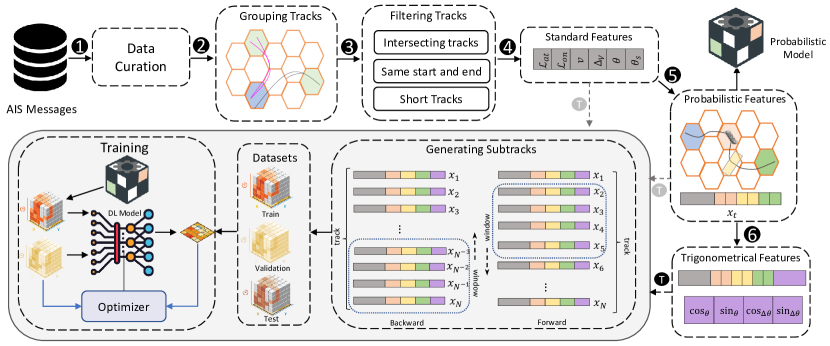
Figure 6: Visual representation of our pipeline. We start with a subset of AIS messages that cover the Gulf of St. Lawrence. After curating the data and separating messages by MMSI into tracks (Step 1), we then create shorter segments (tracks) with end-to-end trip behavior and group these tracks based on common start and end points (Step 2). This means the dataset is divided into subsets with a balanced number of trajectories based on their unique patterns, and then the samples are weighted according to their population. All short tracks, self-intersecting tracks, and tracks having the same start and end port are removed (Step 3). We reverse the tracks and add them to the dataset as new tracks. Using positional attributes, bearing, speed, and their rate of change is calculated to form the Standard Features set (Step 4). This features set is further extended by Probabilistic Features, which are current grid cell (orange color), route polygon (yellow color), and last grid cell (green color) centroids, and for that, we consider the start and end of each track and the closest route polygon placed in the gulf (Step 5). These new features are used for computing the probabilistic model. We then add Trigonometric Features for each message of tracks to extend the existing feature set (Step 6). In Step T, for each track, using the sliding window technique, we generate sub-sequences (trajectories) in contiguous temporal slices of up to 15 hours to construct training, validation, and testing datasets. The first three hours serve as the input to the deep learning model, and the following 12 hours are the observed data to compare to the model prediction. After applying a temporal mini-batch training method, we optimize the neural network to identify the best subset of parameters that can closely forecast the samples in the training set. When training with probabilistic features, each sample is updated to have the additional engineered features from the probabilistic model before feeding to the neural network. This training process is repeated several times until there is no further improvement when testing the model on the validation-reserved data, and after training, we evaluate it on the test data.

In our trajectory forecasting pipeline, depicted in Figure 6, we extract MMSI, timestamps, vessel type, and coordinates from AIS messages recorded between 2015 and 2020. Although over ten types of vessels are included in the data, our study only focuses on cargo and tanker vessels due to their distinguishable linear movement behavior (Step 1). Our pipeline uses tracks, which are ordered sequences of a vessel’s positions from a source port to a destination, instead of complete voyages. Creating tracks from AIS messages involves segmenting voyages based on the time and distance between consecutive messages to identify sub-sequences with end-to-end trip behavior. In our study, a new track starts if the interval between two consecutive AIS messages exceeds 8 hours or the distance interval exceeds 50 Km. We weigh the tracks based on their starting and ending grid, assigning a weight value corresponding to the vessel density of that moving pattern with respect to the entire dataset. Such weight is used for stratified dataset sampling, assuring that distinct mobility patterns will be equally used for model training and validation (Step 2).

In Step 3 of our data processing pipeline, we discard messages within one kilometer of the nearest port as vessels are likely anchored in these areas. Additionally, we discard self-intersecting tracks and tracks that start and end at the same port, often observed in fishing vessels. After this filtering, we interpolate the remaining messages within each track to be 10 minutes apart based on their timestamp. Next, we remove tracks that are outliers from the dataset. Specifically, we identify outlier tracks within a grid cell where the number of tracks of a particular stratification pattern is less than or equal to five. That is the case of tracks of vessels patrolling around marine protected areas that may have been mislabeled during data collection and thus need to be removed. The resulting dataset consists of vessels grouped by their MMSI and divided by their type, with sets of tracks containing only coordinates. Finally, in the preprocessing stage, we reverse the tracks and add them to the dataset as new tracks to increase the sample size for the experiment. In step Step 4, we calculate the speed displacement of the vessel in knots and its acceleration in knots per hour based on the distance between the consecutive AIS messages. We do the same to compute the bearing of the vessel and the rate of the change of the bearing in gradian (see Methods). The resulting information is called the Standard Features of each track. Further, we split a track into two where the rate of change in the bearing between two consecutive points varies by more than $\pm 45^{g}$. The output of this process is divided into training, validation, and testing by vessel type and MMSI.

Afterward, we split the dataset into three subsets: training, validation, and testing. The division is based on vessel type and MMSI, following the stratified sampling weights defined earlier. We use the training set to construct the probabilistic model. This model is capable of identifying common routes and predicting their probable destinations. The presence of multiple routes between frequently traveled source and destination ports highlights the need for creating route polygons to direct the forecasting models. In this sense, the set of Standard Features of each track is extended with the current grid cell, route polygon, and last grid cell centroids (Step 5). We refer to this extended feature set as Probabilistic Features. Subsequently to this step, in Step 6, we further extend the Probabilistic Features by calculating trigonometrical transformation on top of the vessels’ location and bearings resulting in the Trigonometrical Features. Either of the three feature sets can be used for training the deep learning model in Step T, but not multiple simultaneously. For example, in Figure 6, the Trigonometrical Features is the input of the deep learning model, whereas arrows from the other feature sets are greyed out.

To generate smaller sequences of tracks for the deep learning model, we generate trajectories that are up to 15 hours long using a sliding window algorithm. This algorithm processes 3 new messages at a time, iterating over a track every 30 minutes. This aims to ensure that the input data is shaped into vectors of equal size, ranging from 1 to 3 hours, by padding any missing values. The output vectors always have a size of 12 hours, and no padding is applied to them. The deep learning model uses the first 3 hours of the output vector as input, while the remaining 12 hours are observed data used to evaluate the model’s prediction. We proceed to neural network engineering and training after generating the input features normalized between $[0,1]$. Regardless of the feature set we use, we expect the model to generate a pair of normalized coordinates in the range of $[0,1]$ as output, which, when denormalized, should resemble the anticipated output of the vessel trajectory. Such models are trained on the same training data that was used to build the probabilistic model, which is now segmented into trajectories. The training continues until no improvement is seen on the validation-reserved dataset slice, after which the models are evaluated on the test dataset. The training and validation are conducted simultaneously on tankers and cargo vessels. However, the final testing is performed separately so that we can account for the individual performance by vessel type. We also allow the last element in the training input vector to be present as the first element of the output vector (overlap of 10 minutes) to enhance the continuity of the sequential data.

Our experiments involve testing different sets of features and network architectures. Our contributions are on feature engineering and neural network modeling, which together can make complex long-term path decisions. We conducted experiments with three distinct sets of features and displayed the results of other neural network models in an ablation fashion. We covered comparisons with the literature and state-of-art, including simple RNNs [53, 54, 55], Bidirectional RNNs [56, 57, 58], CNNs/RNNs AutoEncoders [59, 60, 61], and combinations of those with and without the transformer-based attention mechanism, all of which have less than 1.5M trainable parameters. We chose not to test models that exceeded the threshold due to their large size and long training time requirements. As AIS is a type of streaming data, it requires models that can train and produce fast outputs. Our proposal suggests using smarter features in combination with simpler, well-tailored models. Additionally, in the context of the Gulf of St. Lawrence, there is not enough data and information available to justify the use of larger and deeper models. These models may not necessarily provide better results but will require more resources and take longer sessions to train and refine.

Differently from the literature, our model uses parallel Convolutional Neural Networks (CNNs) to extract local and global features from input data through dilated convolutions. The CNNs’ outputs are combined and processed by a Bidirectional Long Short-Term Memory (Bi-LSTM) with a Position-Aware Attention mechanism, efficiently encoding the temporal sequence, giving higher importance to later timesteps. The resulting latent space is then decoded through a second Bi-LSTM and multiple Dense layers, giving the final output as normalized latitude and longitude values. This end-to-end, customizable architecture achieves superior performance in predictive geospatial tasks, mainly when trained with the aid of probabilistic and trigonometrical features. To start this discussion, subsequently, we formalize our probabilistic model while using Table 1 to describe the symbols and notations used from hereinafter.

Table 1: Symbols and notations relevant for the probabilistic model formulation understanding.

Notation	Definition
$\tau$	An ordered sequence of $t$ points
$x_{t}$	A point in a $\tau$ at instant $t$, in format $\left<\mathcal{L}_{on},\mathcal{L}_{at},S,\Delta_{v},\theta,\Delta_{\theta}\right>$
$\mathcal{L}_{on}$	Longitude in degrees
$\mathcal{L}_{at}$	Latitude in degrees
$v$	Speed in knots
$\Delta_{v}$	The acceleration in knots per unit time of the vessel
$\theta$	Bearing in gradian
$\Delta_{\theta}$	The rate of change of the bearing in gradian per unit time
$\mathbf{M}$	Route probability matrix $\mathbf{M}\in\mathbb{R}^{c\times r\times z}$, where $c$ is the number of grid cells, $r$ is the number of route polygons and $z$ is number of tracks from $c$ passing through $r$
$\widetilde{\mathbf{M}}$	Destination probability matrix $\widetilde{\mathbf{M}}\in\mathbb{R}^{c\times c\times z}$, where $c$ is the number of grid cells and $z$ is number of tracks passing through a given grid cell
$C$	Set of all grid cells $C=\left\{C_{i}\right\}^{c}_{i=1}$
$D$	Subset of destination grid cells $D=\left\{D_{j}\right\}^{d}_{j=1}$ where $D\subseteq C$
$T$	Collection of tracks $T=\left\{\tau_{i}\right\}^{n}_{i=1}$, where $n$ is the number of tracks
$T_{C_{i}}$	Subset of tracks that have passed through a specific grid cell $C_{i}$
$T_{D_{j}}$	Set of tracks that ended up in $D_{j}$
$S_{\tau}$	A tuple of motion statistics of track $\tau$ in format $\{\mathcal{L}_{f},\mathcal{L}_{e},\widetilde{\theta}_{g},\Psi_{\theta_{g}}\}$
$\mathcal{L}_{f}$	First AIS coordinates of track $\tau_{i}$ within a grid cell $C_{i}$
$\mathcal{L}_{e}$	Last AIS coordinates of track $\tau_{i}$ within a grid cell $C_{i}$
$\widetilde{\theta}_{g}$	The median of the course values of vessel movements in a grid cell
$\Psi_{\theta_{g}}$	The Gaussian Kernel Density Estimation-based entropy of the bearing values
$\delta$	Euclidian distance threshold for motion statistics, first quantile of all pre-computed distances
$\mathbf{I}(\cdot)$	Indicator function, outputs 1 if a $\tau$ satisfies the input conditions, else 0
$E$	Euclidian distance function, as defined in Equation 1
$\mathcal{L}^{R}$	Predicted route centroid coordinates, where $R\subseteq C$
$\mathcal{L}^{N}$	Current grid cell’s centroid coordinates, where $N\subseteq C$
$\mathcal{L}^{D}$	Predicted destination grid cell’s centroid coordinates, where $D\subseteq C$

Probabilistic Features and Probabilistic Model

A trajectory is a sequence of points representing the location of an object over time, and, in this paper, a trajectory $\tau$ is represented as an ordered sequence of $t$ points in time, such as $\tau=\left<x_{1},x_{2},\ldots,x_{t}\right>$, where a point $x_{t}\in\tau$ at time $t$ is also an ordered sequence of features from the AIS message such as $x_{t}=\left<\mathcal{L}_{on},\mathcal{L}_{at},v,\Delta_{v},\theta,\Delta_{\theta}\right>$; where $\mathcal{L}_{on}$ is the longitude, $\mathcal{L}_{at}$ the latitude, $v$ the speed in knots, $\theta$ the bearing in gradian, $\Delta_{v}$ the acceleration in knots per hour, and $\Delta_{\theta}$ the rate of change of the bearing in gradian. We refer to the set of values in $x_{t}$ of each AIS message as Standard Features. The speed, bearing, and deltas can be mathematically calculated using sequences of coordinates (see Methods for details).

Our approach involves probabilistic modeling where we consider a 310-cell grid that overlays the Gulf of St. Lawrence and six-year historical AIS data to create a Route Probability Matrix $\mathbf{M}\in\mathbb{R}^{c\times r\times z}$ and a Destination Probability Matrix $\widetilde{\mathbf{M}}\in\mathbb{R}^{c\times c\times z}$. Here, $c$ represents the number of cells, $r$ is the number of possible routes (route polygons), and $z$ is the number of tracks passing through a grid cell or route polygon. Through those, we aim to generate a probable route and destination that can be used as features for deep-learning models to forecast vessels’ trajectories. It is important to note that our probabilistic model does not predict the next grid cell of the vessel during the vessel displacement in the trajectory. Instead, it predicts the probable long-term decisions that vessels will make. In the end, we will have a collection of conditional probabilities related to trajectories $T$, grid cells $C$, and destination grid cells $D$. We use $T_{C_{i}}$ to refer to a subset of tracks that have passed through a particular grid cell $C_{i}$ and $T_{D_{j}}$ to represent the set of tracks that ended up in $D_{j}$, $i\neq j$. For a simple conditional probability formulation where $z$, the individual tracks interacting with the grid cells, is not taken into account, one could populate $\mathbf{M}_{ij}$ with the conditional probability of tracks crossing a route polygon $R_{k}$ given it crossed the grid cell $C_{i}$ as $\mathbb{P}(R_{k}|C_{i})=|T_{R_{k}}\cap T_{C_{i}}|\div|T_{C_{i}}|$ and populate $\widetilde{\mathbf{M}}_{ij}$ with the conditional probability of a trajectory crossing a grid cell $D_{j}$ given it crossed the grid cell $C_{i}$ as $\mathbb{P}(D_{j}|C_{i})=|T_{D_{j}}\cap T_{C_{i}}|\div|T_{C_{i}}|$.

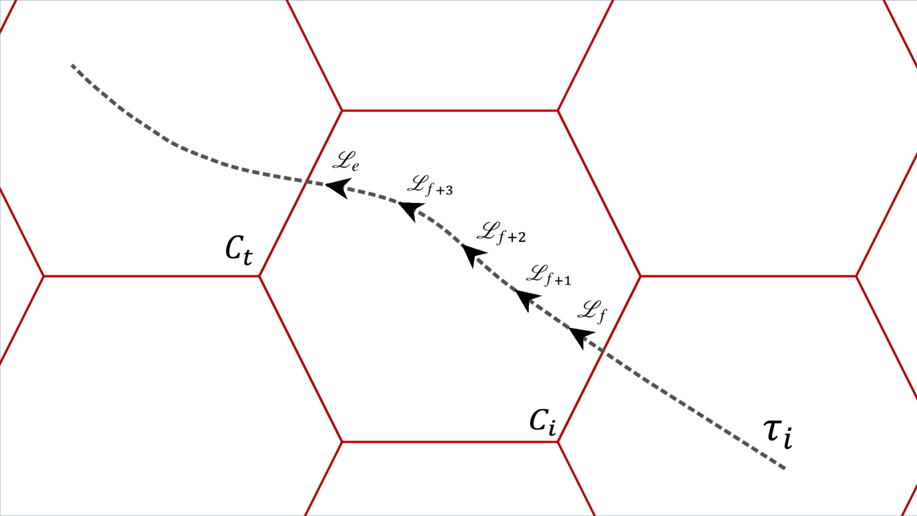
Figure 7: An example of AIS coordinates $\mathcal{L}_{f}$ first and $\mathcal{L}_{e}$ last of a vessel inside a grid cell $C_{i}$ (current) and $C_{t}$ (subsequent) on the vessel trajectory $\tau_{i}$.

Unfortunately, conditional probabilities alone cannot accurately describe the transition between grid cells. This would lead to a bias towards shipping routes with higher vessel traffic over time. Moreover, assuming an equal distance between all grid cells neglects the importance of the vessel course and its distance (from the last AIS message location) to the nearest route polygon. Because of that, we consider the relationship of the vessel location with the route polygon. We do so by accounting for the trajectory $\tau_{i}$ movement direction while passing through $C_{i}$, as depicted in Figure 7. Such directional information ($S_{\tau_{i}}$) is stored on the last axis of our probability matrices $\mathbf{M}\leavevmode\nobreak\ /\leavevmode\nobreak\ \widetilde{\mathbf{M}}$, for each destination grid cell and route polygon, respectively. We refer to the motion direction ($S_{\tau_{i}}$) as motion statistics. The motion statistics for each track $\tau_{i}\in T_{C_{i}}$ consist of a four-value tuple, which is represented by $S_{\tau_{i}}=\{\mathcal{L}_{f},\mathcal{L}_{e},\widetilde{\theta}_{g},\Psi_{\theta_{g}}\}$. Within $C_{i}$, $\mathcal{L}_{f}$ and $\mathcal{L}_{e}$ represent the first and last pair of coordinates, respectively, of $\tau_{i}$ — e.g., $\mathcal{L}_{f}=\Big{<}\mathcal{L}_{lon}^{f},\mathcal{L}_{lat}^{f}\Big{>}$; $\widetilde{\theta}_{g}$ is the median of the course values; and, $\Psi_{\theta_{g}}$ is the Gaussian Kernel Density Estimation-based entropy of the course values within the messages inside $C_{i}$. A hexagonal grid cell has geometrically six neighbors, and $\Psi_{\theta_{g}}$ is responsible for capturing the movement and change in the direction of the vessel inside a particular grid cell. Each $S_{\tau_{i}}$ of historical track is associated with a route polygon $S_{\tau_{i}}\rightarrow R_{k}$ and a destination $S_{\tau_{i}}\rightarrow D_{\tau_{i}}$, in which, motion statistic for each track $\tau\in T$ is computed. The idea behind this approach is to define feasible transitions between routes’ and destinations’ grid cells.

The similarity of a new trajectory $\tau_{n}$ and an existing historical track $\tau_{i}$ in a given grid cell $C_{i}$ is computed using Euclidean distance of their motion statistics $S^{C_{i}}_{\tau_{n}}$ and $S^{C_{i}}_{\tau_{i}}$, respectively, in $C_{i}$ using equation:

$$\hfill E\left(S^{C_{i}}_{\tau_{n}},S^{C_{i}}_{\tau_{i}}\right)=\sqrt{\left(\mathcal{L}_{f}^{\tau_{n}}-\mathcal{L}_{f}^{\tau_{i}}\right)^{2}+\left(\mathcal{L}_{e}^{\tau_{n}}-\mathcal{L}_{e}^{\tau_{i}}\right)^{2}+\left(\widetilde{\theta}_{g}^{\tau_{n}}-\widetilde{\theta}_{g}^{\tau_{i}}\right)^{2}+\left(\Psi_{\theta_{g}}^{\tau_{n}}-\Psi_{\theta_{g}}^{\tau_{i}}\right)^{2}}\hfill$$ (1)

where $\mathcal{L}_{f}$ and $\mathcal{L}_{e}$ represent starting and ending coordinates; and, $\widetilde{\theta}_{g}$ and $\Psi_{\theta_{g}}$ refer to the median and entropy of bearing values, respectively. The distance is calculated between the current track $\tau_{n}$ and each historical track $\tau_{i}$ inside grid cell $C_{i}$. In this calculation, every value in $S_{\tau}$ is normalized between the range $[0,1[$, which ensures that all features have equal influence on the distance measure. The lower the Euclidean distance, the more likely a vessel will take that route or reach its more probable destination.

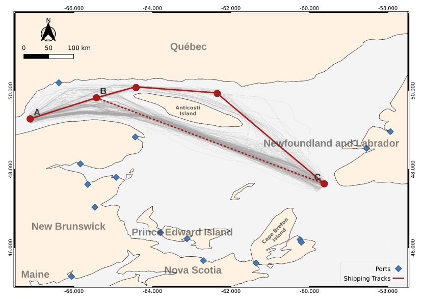
(a)

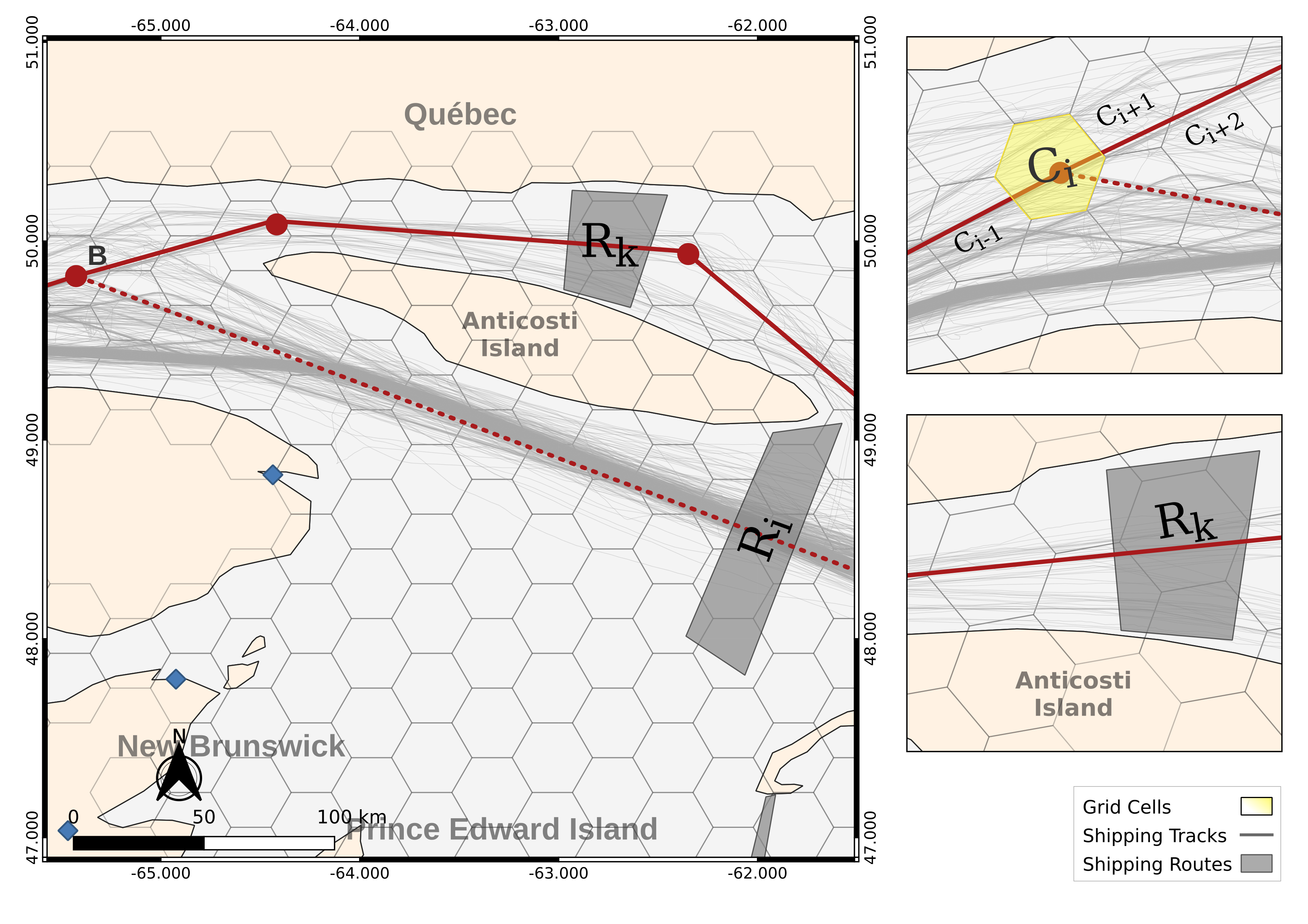
(b)

Figure 8: The image (a) displays a density map depicting two routes from a starting point A towards the endpoint C. In image (b), the region has been divided into hexagonal grid cells of 0.3^o using ESPG:4269 projection, where a grid cells are referred to as $C_{i}$ and possible routes as $R_{i}$ and $R_{k}$. The solid red line shows the probable movement of a vessel between B and C, and the dashed line shows a less probable one.

As an example of the probabilistic process, Figure 8 depicts a vessel moving from point A to C, with a decision point at the segment between point B and C. At this decision point, there are two possible paths, each of which interacts with a different route polygon ($R_{i}$ and $R_{k}$). The solid red line represents the most probable path, while the dashed line shows the least probable path. To define a probable route of a vessel, we need to consider the location of the route polygon ($R_{k}$ or $R_{i}$), the vessel’s location ($C_{i}$) during track $\tau_{n}$, and the motion statistics. We define the probability function for choosing a route as follows:

$$\hfill\mathbb{P}(R_{k}|C_{i},\tau_{n})=\frac{\sum_{\tau_{i}\in T}\mathbf{I}\Big{(}x_{t}\in\tau_{i}\wedge\exists x_{t}\in R_{k}\,\wedge\,E(S_{\tau_{n}},S_{\tau_{i}})\leq\delta\,\wedge\,\exists x_{t}\in C_{i}\Big{)}}{\sum_{\tau_{i}\in T}\mathbf{I}\Big{(}x_{t}\in\tau_{i}\,\wedge\,E(S_{\tau_{n}},S_{\tau_{i}})\leq\delta\,\wedge\,\exists x_{t}\in C_{i}\Big{)}};\hfill$$ (2)

where $\delta$ is a threshold representing the first quantile value of all pre-computed distances between historical motion statistics as defined in Algorithm 1, explained in the Methods section. Additionally, the probability for the destination $D_{j}$ is formalized with respect to the route polygon $R_{k}$, using the following equation:

$$\hfill\mathbb{P}(D_{j}|C_{i},R_{k},\tau_{n})=\frac{\sum_{\tau_{i}\in T}\mathbf{I}\Big{(}x_{t}\in\tau_{i}\,\wedge\,\exists x_{t}\in D_{j}\,\wedge\,E(S_{\tau_{n}},S_{\tau_{i}})\leq\delta\,\wedge\,\exists x_{t}\in C_{i}\,\wedge\,\exists x_{t}\in R_{k}\Big{)}}{\sum_{\tau_{i}\in T}\mathbf{I}\Big{(}x_{t}\in\tau_{i}\,\wedge\,E(S_{\tau_{n}},S_{\tau_{i}})\leq\delta\,\wedge\,\exists x_{t}\in C_{i}\,\wedge\,\exists x_{t}\in R_{k}\Big{)}};\hfill$$ (3)

in cases where the route polygons are known not to interact with the historical tracks, such as in the case of Figure 4(c), we can simplify the conditional probabilistic destination model from above as follows:

$$\hfill\mathbb{P}(D_{j}|C_{i},\tau_{n})=\frac{\sum_{\tau_{i}\in T}\mathbf{I}\Big{(}x_{t}\in\tau_{i}\,\wedge\,\exists x_{t}\in D_{j}\,\wedge\,E(S_{\tau_{n}},S_{\tau_{i}})\leq\delta\,\wedge\,\exists x_{t}\in C_{i}\Big{)}}{\sum_{\tau_{i}\in T}\mathbf{I}\Big{(}x_{t}\in\tau_{i}\,\wedge\,E(S_{\tau_{n}},S_{\tau_{i}})\leq\delta\,\wedge\,\exists x_{t}\in C_{i}\Big{)}};\hfill$$ (4)

Equations 2, 3, and 4 take into account all the tracks in the dataset. The selection of tracks in the numerator and denominator is guided by the indicator function $\mathbf{I}(\cdot)$, which outputs 1 if a $\tau_{i}$ satisfies all conditions.

Equation 2 is defined in terms of the ratio of total historical tracks that have visited $C_{i}$ out of which tracks have visited $R_{k}$. In other words, a track for the indicator function is selected if: (a) any point $x_{t}$ of track $\tau_{i}$ falls within the route polygon $R_{k}$ and $C_{i}$; and (b) the Euclidean distance $E$ of motion statistics within $C_{i}$ is less than a threshold $\delta$. Equation 3 considers the destination probability with respect to the intersection with a route polygon $R_{k}$, which has the same criteria as in Equation 2 but with a change in (b): a point within the track falls into the destination cell $D_{j}$, instead of the route polygon. For Equation 4, which calculates destination probability without considering an interacting route polygon, the criteria are much the same as 2 and 3, but it no longer requires a point in the track to fall into the route polygon $R_{k}$.

The proposed models use conditional probability to add new features to vessel trajectory data. These features, called Probabilistic Features, provide additional information, such as the predicted route polygon and destination grid cell for each trajectory. The new features are obtained by converting transition probabilities into weighted similarity scores and those into cell-grid centroids, which are then added to the AIS messages within the vessel track. For example, a point $x_{t}$ at time $t$ from a track $x\in\tau$ is now known to be of shape $x_{t}=\left<\mathcal{L}_{on},\mathcal{L}_{at},v,\Delta_{v},\theta,\Delta_{\theta},\mathcal{L}_{on}^{R},\mathcal{L}_{at}^{R},\mathcal{L}_{on}^{N},\mathcal{L}_{at}^{N},\mathcal{L}_{on}^{D},\mathcal{L}_{at}^{D}\right>$. Here, $\mathcal{L}^{R}$ indicates the centroid coordinates of the route polygon if the track is predicted to intersect with at least one of the known routes; $\mathcal{L}^{N}$ indicates the centroid coordinates of the grid cell where the vessel currently lies; and, $\mathcal{L}^{D}$ indicates the coordinates of the destination grid cell of the track; where, $C$ is all grid cells, $R\subseteq C$, $N\subseteq C$ and $D\subseteq C$.

Defining the final set of features relies on conditions that depend on the number of routes identified in the dataset and the intersection of the trajectories of interest with the route polygons. In this sense, defining $\mathcal{L}^{D}$, which is the same for an entire track, depends on a similarity-based score calculation:

$$\hfill\mathbb{S}(D_{j}|C_{i},S_{\tau})=\begin{cases}\xi\times\mathbb{P}(D_{j}|C_{i},R_{k},S_{\tau})&\text{if}\,\,\mathbf{max}_{k}[\xi\times\mathbb{P}(R_{k}|C_{i},S_{\tau})]>0,\\ \xi\times\mathbb{P}(D_{j}|C_{i},S_{\tau})&\text{otherwise}.\end{cases}\hfill$$ (5)

Here, $\xi=\left(1-E\left(S_{\tau_{n}},S_{\tau_{i}}\right)\right)$ is the similarity value calculated based on the Euclidian distance. The destination of a track is conditional to the existence of a route polygon that interacts with the trajectory or is independent of it otherwise; knowing that $C_{i}$ is where the vessel lies, $D_{j}$ is the possible destination within any of the 310 cells, and $R_{k}$ is one of the 4 route polygons previously identified in the gulf. Differently, defining $\mathcal{L}^{R}$, which is also shared with the entire track, depends on the next equation:

$$\hfill\mathbb{S}(R|C_{i},S_{\tau})=\begin{cases}\mathbf{max}_{k}[\xi\times\mathbb{P}(R_{k}|C_{i},S_{\tau})]&\text{if}\,\,\mathbf{max}_{k}[\xi\times\mathbb{P}(R_{k}|C_{i},S_{\tau})]>0,\\ \mathbf{max}_{j}[\xi\times\mathbb{P}(D_{j}|C_{i},S_{\tau})]&\text{otherwise}.\end{cases}\hfill$$ (6)

such a case takes into consideration that not all tracks interact with a known route polygon, and whenever this happens, the centroid of the route polygon $\mathcal{L}^{R}$ is replaced by the centroid of the most probable destination $\mathcal{L}^{D}$ among the grid cell in the gulf to increase the robustness of the probabilistic model.

Trigonometrical Transformations

Predictive modeling for trajectory data presents challenges in representing geospatial data when measured in degrees or gradians, such as for longitude, latitude, and bearing. Traditional Recurrent Neural Networks, including Long Short-Term Memory (LSTM) networks, may not be able to properly interpret these variables’ cyclical and cardinal nature when directly used in learning, even if $[0,1]$ normalized. This can result in artificially induced discontinuities and misinterpreted spatial relationships within the dataset. That is because the degree space is not contiguous with the physical space, as is the case of the Cartesian plane.

To better handle degree-based data, it is helpful to use transformations that maintain their inherent cyclical relationships. When dealing with longitude and latitude values, we can project them onto a unit sphere (i.e., radius one). This mapping method transforms the data onto a three-dimensional surface while encoding its geodesic similarities into a nearly Cartesian space using the following sequence of equations:

$$\hfill\begin{aligned} \alpha&=\cos\Big{(}\mathcal{L}_{on}\Big{)}\times\cos\Big{(}\mathcal{L}_{at}\Big{)}\\ \beta&=\sin\Big{(}\mathcal{L}_{on}\Big{)}\times\cos\Big{(}\mathcal{L}_{at}\Big{)}\\ \gamma&=\sin\Big{(}\mathcal{L}_{at}\Big{)}\end{aligned}\hfill$$ (7)

where $\mathcal{L}_{on}$ is the longitude and $\mathcal{L}_{at}$ is the latitude, and $\alpha,\beta,\gamma\in[0,1]$. This type of transformation is designed to maintain the spatial relationships between points on the Earth’s surface, ensuring that nearby points remain adjacent in the transformed representation. However, it becomes inaccurate when dealing with data that are located too close to the Earth’s poles, such as in the Arctic Ocean. Unlike coordinates, bearing values cannot be projected directly onto a Cartesian space. However, they can be transformed using cosine and sine functions, which enable a sinusoidal representation of the data.

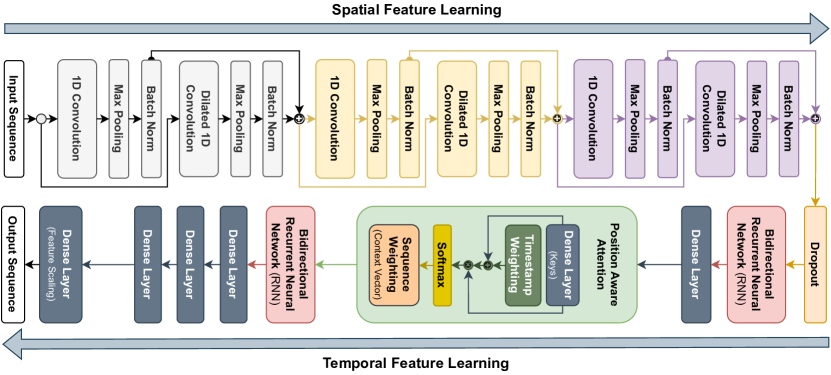
Figure 9: The proposed deep-learning model uses parallel convolutions and a sequential stack of convolution blocks to capture short and long-term spatial features. The extracted features are passed through a dropout layer and a Bi-LSTM with a fully connected layer. The Position-Aware Attention mechanism enhances the importance of later timestamps. The final encoded latent space undergoes a Bi-LSTM decoding phase and a multi-layer fully connected network to produce normalized coordinates.

Table 2: Symbols and notations relevant for the deep-learning model formulation understanding.

Notation	Definition
$b$	Batch size of the input tensor
$w$	Window size of the input, which represents the number of timestamps
$v$	Number of features in each input timestamp
$f$	Size of convolution filters
$s$	Stride of convolution layers
$m$	Number of filters in convolution layers
$\mathbf{x}$	Input tensor to the model, of shape $\mathbb{R}^{b\times w\times v}$
$\mathbf{W}$	Representation of the weights of the model layers
b	Representation of the bias parameters of the model layers
$\star$	Cross-correlation operator used by single-dimensional convolutions
$\widetilde{w}$	Reduced size of window after convolution
$\epsilon$	Small constant to avoid division by zero
$\mu_{b}^{d}$, $(\sigma_{b}^{d})^{2}$	Mean and variance for each filter $d$ within batch $b$ in batch normalization
$\gamma^{\leavevmode\nobreak\ d}$, $\beta^{d}$	Scaling and shifting parameters for each filter $d$ in batch normalization
$h$	Size of max pooling filter
$d$	Feature dimensions – changes with each iteration through layers
$\vartheta$	Dilation factor for kernel expansion in dilated convolutions
$\mathbf{C}$, $\widetilde{\mathbf{C}}$	Cell state and candidate cell state of the Bi-LSTM
$\mathbf{i}$, $\mathbf{f}$	Input gate and forget gate of the Bi-LSTM
$\mathbf{o}$, $\mathbf{h}$	Output gate and hidden state of the Bi-LSTM
$\sigma(\cdot)$	Sigmoid activation function of the Bi-LSTM
$\phi(\cdot)$	Activation function used in the model (i.e., ReLU)
$(\cdot)\%(\cdot)$	Integer part of the rest of the division between two numerical values
$\mathbf{A}$	Attention weights for Position-Aware Attention mechanism
$\mathbf{E}$	Position-Aware context vector of shape $\mathbb{R}^{b\times z\times d}$
$\otimes$	Tensor repeating and concatenation operator
$\omega$	Time factor for establishing a focal point in attention mechanism
$z$	Window size of the output, which represents the number of output timestamps
$\Xi(\cdot)$	Re-scaling function for coordinate values generation
$\mathbf{y}$	Final output tensor representing latitude and longitude, of shape $\mathbb{R}^{b\times z\times 2}$

For speed, applying the logarithmic transformation can be effective, especially when dealing with values spanning across multiple orders of magnitude. This can ensure that larger-scale patterns do not overly influence the model, allowing local trends to play a part in the decision-making process. This can be achieved with the equation $v^{\prime}=\log(1+|v|)$, where $v^{\prime}$ is the transformed and $v$ is the original speed. Through these sets of transformations, the earlier point $x$ at time $t$ from a trajectory $\tau$ become $x_{t}=\Big{<}\mathcal{L}_{on},\mathcal{L}_{at},\alpha,\beta,\gamma,v,\Delta_{v},\theta,\Delta_{\theta},v^{\prime},\Delta_{v^{\prime}},\cos_{\theta},\sin_{\theta},\cos_{\Delta_{\theta}},\sin_{\Delta_{\theta}},\mathcal{L}_{on}^{R},\mathcal{L}_{at}^{R},\alpha^{R},\beta^{R},\gamma^{R},\mathcal{L}_{on}^{N},\mathcal{L}_{at}^{N},\alpha^{N},\beta^{N},\gamma^{N},$ $\mathcal{L}_{on}^{D},\mathcal{L}_{at}^{D},\alpha^{D},\beta^{D},\gamma^{D}\Big{>}$. This final representation includes Standard, Probabilistic, and Trigonometrical Features. It provides an enriched input dataset for the deep-learning model tailored for trajectory forecasting, facilitating its understanding of complex spatial and temporal patterns of the trajectories. With all feature sets properly defined, we move forward with the formalization of the deep-learning model (see Figure 9), which is based on Table 2 for describing the symbols and notations used from hereinafter.

Deep Learning Model

The deep learning model comprises two main parts; spatial and temporal feature learning, as depicted in Figure 9. Our customized architecture uses parallel convolutional neural networks with recurrent neural networks and focal attention for position-aware temporal learning. During the model formulation, we use lower-case bold letters to represent vectors, such as $\mathbf{x}$, upper-case bold letters to represent matrices, such as $\mathbf{W}$, and non-bold lower-case values, such as $b$, to indicate a scalar value or an integer index of matrices and vectors. The equations are defined with indices to help understand how the data changes as it flows through the architecture and to indicate the meaning of each process accomplished by the network module. We use $\mathbf{x}$ to describe the input tensor, which is propagated and updated at each process step. The weights and biases, $\mathbf{W}$ and $\mathbf{b}$, are independent of each other but are optimized together during the network training.

Giving an input tensor $\mathbf{x}\in\mathbb{R}^{b\times w\times v}$, where $b$ denotes the batch size, $w$ denotes the window size of the input vectors, and $v$ denotes the number of features. Our model begins by executing single-dimensional parallel convolutions. Essentially, we slide a filter (also known as a kernel) of size $f$ across each window element and calculate the dot product across all features with a stride of $s$ for each filter $m$. This way, we process the input tensor to extract spatial features that will be used in subsequent model layers.

$$\hfill\mathbf{x}_{b,i,m}=\sum_{j=1}^{f}\sum_{n=1}^{v}\mathbf{x}_{b,(i+(s\times(j-1))),n}\cdot\mathbf{W}_{m,j,n}\equiv\mathbf{x}_{b,i}\star\mathbf{W}_{m}\hfill$$ (8)

Based on the filter size $f$ and stride $s$, we follow this operation for each window element to yield an output tensor $\mathbf{x}\in\mathbb{R}^{b\times\widetilde{w}\times m}$, where $\widetilde{w}$ represents the new window size and $m$ denotes the kernel size. The cross-correlation $\star$ operation represents an equivalent of this convolution. The convolutional layers play a crucial role in extracting spatial features of the input trajectories, especially for long-term trajectory forecasting. These layers are particularly helpful when the input data is limited to short-term data. They can learn spatial patterns like curves and slight course changes based on historical data, but they tend to overfit the input data and can only learn patterns that fit their kernel size (short or long-term dependencies).

Subsequently, $\mathbf{x}\in\mathbb{R}^{b\times\widetilde{w}\times m}$ goes through batch normalization to fit the values of the resulting tensor into a standard scale. This is followed by a max-pooling operation, and the two processes are defined as:

$$\hfill\mathbf{x}_{b,i,m}=\mathbf{max}\left(\frac{\mathbf{x}_{b,p,m}-\mu_{b}^{d}}{\sqrt{\big{(}\sigma_{b}^{d}\big{)}^{2}+\epsilon}}\cdot\gamma^{\leavevmode\nobreak\ d}+\beta^{d}\right)\quad\forall p\in[i,i+h-1]\hfill$$ (9)

For each filter $m$ and batch $b$, a window of size $h$ is defined on the feature map starting at position $i$, with the condition that $i+h-1\leq\widetilde{w}$. The filter-wise mean $\mu_{b}^{d}$ and variance $\big{(}\sigma_{b}^{d}\big{)}^{2}$ are calculated for batch $b$, along with specific scaling $\gamma^{\leavevmode\nobreak\ d}$ and shifting $\beta^{d}$ parameters. Next, the max pooling operation is performed over the window, extracting the maximum value of $p$. The resulting value is assigned to $\mathbf{x}_{b,i,d}$, which becomes the feature map for the given window of filter index $d$. Due to working with parallel convolutions that involve different kernel sizes, it is necessary to use a combination of techniques to ensure consistent tensor dimensions. We use batch normalization and max-pooling to scale down the tensor dimensions into shared tensor dimensions with scaled values, which can be merged later. This approach guarantees that the branches can be combined seamlessly without stability issues during the training.

As mentioned, single-dimensional CNNs can only learn spatial features within their kernel size. We employ parallel convolutions in residual blocks to capture both short-term and long-term spatial features simultaneously. This is achieved through dilated convolutional layers, which expand the kernel size by a factor of $\vartheta$ and enable it to capture extended spatial features from the input data. Both convolutional branches in a block are trained together, but they work independently on copies of the input data such that they are not affected by each other. To perform dilated convolution, we modify Equation 8 as follows:

$$\hfill\mathbf{x}_{b,i,m}=\sum_{j=1}^{f}\sum_{n=1}^{v}\mathbf{x}_{b,(i+(s\times\vartheta\times(j-1))),n}\cdot\mathbf{W}_{m,j,n}\equiv\mathbf{x}_{b,(i+\vartheta)}\star\mathbf{W}_{m}\hfill$$ (10)

where $j$ stands for the filter index, and $\vartheta\times(j-1)$ is the expansion of the kernel due to the dilation rate $\vartheta$. The resulting output of the branches, given by Equation 9, is then combined into a single tensor as such:

$$\hfill\mathbf{x}_{b,i,m}=\mathbf{x}_{b,i,m}^{T}+\mathbf{x}_{b,i,m}^{D}\hfill$$ (11)

where $T$ and $D$ denote the results obtained from the traditional and dilated convolution operations.

The series of mathematical operations that end in Equation 11, as shown in Figure 9, is repeated three times, each time with different parameters. At this point, $\widetilde{w}$ and $m$ have dimensions according to the hyperparameters of the convolution block (see Methods). This stack allows us to extract more precise long and short-term spatial features from the input data at each process step. The parallel CNNs and the sequential blocks work simultaneously to produce a refined output of spatial features that is then sent to the next block for further processing, minimizing further the overall error for the forecasting task.

The subsequent part is where the network learns the temporal features from the input data. It starts with a dropout layer to prevent overfitting from the spatial feature data. The dropout layer comprises a binary mask of shape $\mathbb{R}^{b\times\widetilde{w}\times m}$, where each element has a value of 1 with probability $p$ and a value of 0 with probability $1-p$, which is element-wise multiplied with the input data to generate the output. Such output is forwarded to a Bidirectional Long-Short Term Memory (Bi-LSTM) network, which takes $\mathbf{x}\in\mathbb{R}^{b\times\widetilde{w}\times m}$ as input and produces the hidden state $\mathbf{h}_{b,i,r}\in\mathbb{R}^{b\times\widetilde{w}\times r}$ for each time step $i\leq\widetilde{w}$, where $r$ is the dimension of the LSTM inner weights. The Bi-LSTM equations can be formulated as follows:

$$\hfill\begin{aligned} \mathbf{i}_{b,i,r}&=\sigma\Big{(}\mathbf{W}_{i}\cdot\Big{[}\mathbf{h}_{b,(i-1),r}\leavevmode\nobreak\ ,\leavevmode\nobreak\ \mathbf{x}_{b,i,m}\Big{]}+\mathbf{b}_{i}\Big{)}\\ \mathbf{f}_{b,i,r}&=\sigma\Big{(}\mathbf{W}_{f}\cdot\Big{[}\mathbf{h}_{b,(i-1),r}\leavevmode\nobreak\ ,\leavevmode\nobreak\ \mathbf{x}_{b,i,m}\Big{]}+\mathbf{b}_{f}\Big{)}\\ \widetilde{\mathbf{C}}_{b,i,r}&=\mathbf{tanh}\Big{(}\mathbf{W}_{C}\cdot\Big{[}\mathbf{h}_{b,(i-1),r}\leavevmode\nobreak\ ,\leavevmode\nobreak\ \mathbf{x}_{b,i,m}\Big{]}+\mathbf{b}_{C}\Big{)}\\ \mathbf{o}_{b,i,r}&=\sigma\Big{(}\mathbf{W}_{o}\cdot\Big{[}\mathbf{h}_{b,(i-1),r}\leavevmode\nobreak\ ,\leavevmode\nobreak\ \mathbf{x}_{b,i,m}\Big{]}+\mathbf{b}_{o}\Big{)}\\ \mathbf{C}_{b,i,r}&=\mathbf{f}_{b,i,r}\cdot\mathbf{C}_{b,(i-1),r}+\mathbf{i}_{b,i,r}\cdot\widetilde{\mathbf{C}}_{b,i,r}\\ \mathbf{h}_{b,i,r}&=\mathbf{o}_{b,i,r}\cdot\mathbf{tanh}\Big{(}\mathbf{C}_{b,i,r}\Big{)}\\ \mathbf{x}_{b,i,r}&=\phi\Big{(}\mathbf{W}_{d}\cdot\Big{[}\mathbf{h}_{b,i,r}^{\rightarrow}+\mathbf{h}_{b,i,r}^{\leftarrow}\Big{]}+\mathbf{b}_{d}\Big{)}\end{aligned}\hfill$$ (12)

where $\sigma$ is the sigmoid function, $\mathbf{tanh}$ is the hyperbolic tangent function, $[\mathbf{h}_{b,(i-1),r}\leavevmode\nobreak\ ,\leavevmode\nobreak\ \mathbf{x}_{b,i,m}]$ is the concatenation of the previous hidden state with the $i$-th element of the input. $\mathbf{i}$, $\mathbf{f}$, $\widetilde{\mathbf{C}}$, $\mathbf{o}$, $\mathbf{C}$, and $\mathbf{h}$ represent the input gate, forget gate, candidate cell state, output gate, cell state, and hidden state, respectively. $\mathbf{x}_{b,i,r}$ is the output of the process, where $\mathbf{W}_{d}$ and $\mathbf{b}_{d}$ is the weight and bias for the dense layer after the Bi-LSTM and $\phi$ is the ReLU activation. Because Bi-LSTMs compute the hidden states in the forward $\mathbf{h}_{b,i,r}^{\rightarrow}$ and backward $\mathbf{h}_{b,i,r}^{\leftarrow}$ direction, the double output is merged before going through the fully-connected layer.

The next step of this process is to have the output of the fully connected layer undergo the focal version of the attention mechanism. As previously explained, due to working with sequences in which the order is essential, paying greater attention to later timestamps is more critical than early timestamps in the sequence. As such, we use a Position-Aware Attention mechanism that we propose for this use case, a further contribution of this paper. Given the input tensor $\mathbf{x}_{b,i,r}$, where $\mathbf{x}\in\mathbb{R}^{b\times\widetilde{w}\times r}$, our model follows as:

$$\hfill\begin{aligned} \mathbf{K}_{b,i,r}&=\mathbf{x}_{b,i,r}\cdot\mathbf{W}_{b,i,r}+\mathbf{b}_{b,i,r}\\ \mathbf{S}_{b,i,r}&=\mathbf{K}_{b,i,r}\cdot\Big{(}\mathbf{K}_{b,i,r}+\left(\omega\cdot(i\leavevmode\nobreak\ \%\leavevmode\nobreak\ w)\right)\Big{)}\\ \mathbf{A}_{b,i,r}&=softmax\Big{(}\mathbf{S}_{b,i,r}\Big{)}\\ \mathbf{E}_{b,z,r}&=\left(\sum_{i=1}^{w}\mathbf{A}_{b,i,r}\cdot\mathbf{x}_{b,i,r}\right)\otimes 1_{z}\end{aligned}\hfill$$ (13)

In Equation 13, the attention keys are denoted by $\mathbf{K}_{b,i,m}\in\mathbb{R}^{b\times w\times d}$; and, to establish the focal point of attention, we compute a monotonically increasing score in respect to the index of the input tensor $i$ and the time factor $\omega$. We apply the dot product operation on the temporal-scaled samples to get the intermediate scores $\mathbf{S}_{b,i,r}$, followed by a softmax function to get the attention weights $\mathbf{A}_{b,i,r}$. Finally, we calculate the context vector $\mathbf{E}_{b,r}$ by performing a weighted summation of input vectors with the attention weights along with the temporal axis $i$. The context vector is then repeated $z$ times to produce the encoded latent space representation $\mathbf{E}_{b,z,r}$ that will be decoded in the following by the subsequent layers of the model.

After the attention mechanism output (i.e., context vector) has been created, it needs to be decoded to produce meaningful positional results. That is because, at this point, all the timestamps have the same value. The output of the attention mechanism is fed into a new Bi-LSTM with a similar formulation as in Equation 12. The difference in the decoding part is that the hidden states $\widetilde{\textbf{h}}_{b,z,r}\in\mathbb{R}^{b\times z\times\tilde{r}}$ of the Bi-LSTM goes through three fully connected layers instead of one, each of which can be represented as:

$$\hfill\textbf{x}_{b,z,r}^{k}=\phi^{k}\left(\textbf{W}_{d}^{k}\cdot\widetilde{\textbf{h}}_{b,z,r}+\textbf{b}_{d}^{k}\right)\hfill$$ (14)

where $\phi^{k}$ is the activation function, $\textbf{W}_{d}^{k}$ and $\textbf{b}_{d}^{k}$ are the weight matrix and the bias for the $k^{th}$ fully connected layer, respectively. $\textbf{x}_{b,z,d}^{k}$ is the output of the $k^{th}$ fully connected layer, where $k=1,2,3$, $z$ is the timestamps in the temporal axis, and $d$ the transformed feature dimensions matching the size of the weights of the last fully connected layer. To produce the final set of forecasted coordinates, $\textbf{x}_{b,z,r}^{3}$, needs to undergo a last transformation to reduce the axis $d$ into a fixed size of 2, representing the longitude and latitude values:

$$\hfill\textbf{y}_{b,z,\tilde{d}}=\Xi\left(\textbf{W}_{o}\cdot\textbf{x}_{b,z,d}^{3}+\textbf{b}_{o}\right)\hfill$$ (15)

where $\textbf{y}_{b,i,\tilde{d}}\in\mathbb{R}^{b\times z\times 2}$ and $\Xi$ is a custom re-scaling out function that can map the raw output values defined in $[0,1]$ into the valid range of latitude $[-90,90]$ and longitude $[-180,180]$ coordinate values. Due to working with a particular focus on the Gulf of St. Lawrence, our re-scaling function decodes the normalized values in the range $[-68,45]$ for latitude and $[-58,50]$ for longitude of the coordinate values.

Results

The evaluation of results begins with the probabilistic features, which constitute the foundation of our proposal and the main catalyst for improved decision-making using neural networks in the task of multi-path long-term vessel trajectory forecasting. The probability model is trained on the same dataset that will be later used to train the deep-learning model. The crucial difference is that the deep-learning model’s success hinges on the probabilistic model’s successful implementation. The probabilistic model is responsible for feature engineering, while the deep-learning model focuses on trajectory forecasting based on the vessel position and its relevant probabilistic features. This means that when the deep-learning model has access to data regarding the vessel’s probable route and destination, it can significantly decrease the uncertainty in trajectory forecasting, leading to better performance for the forecasting pipeline.

Probabilistc Model Results
Test Type	Coordinate Type	Precision (%)	Recall (%)	F1 Score (%)
Cargo Test	Route	83.13	83.16	81.19
	Destination	75.28	79.09	75.85
Tanker Test	Route	86.89	89.92	87.84
	Destination	74.85	77.12	74.90
Cargo Train	Route	81.69	83.25	80.43
	Destination	89.51	89.72	89.02
Tanker Train	Route	83.43	84.29	82.31
	Destination	88.64	87.95	87.48

Table 3: Performance of the probabilistic model in forecasting a vessel’s route and destination.

The performance evaluations of the probabilistic model across all data segments, for both training and testing datasets, are presented in Table 3. We present the results over the training data for the probabilistic model as it is rule-based and does not store training data. The overperformance observed in the training datasets — especially in forecasting the destinations of the trajectories that scored 89% and 87% F1 Score for cargo and tanker vessels, respectively — are expected outcomes. Forecasting routes in both cases also yield reasonable results, achieving 80% and 82%. More impressively, when utilizing the test data — entirely unseen for the model — the outcome for route forecasting exceeded those observed during the training phase, scoring 81% and 87% for cargo and tanker vessels, respectively. However, regarding destination forecasting, we see a consistent decrease in performance, with the scores dropping to 75% and 74%, respectively. The observed performance difference between the training and testing datasets is an expected behavior – details about the metrics can be found in the Methods section. Even considering these variations, the results obtained are consistent, advocating for the effectiveness of the probabilistic model.

To evaluate the features’ performance in the deep learning model, we conducted experiments that compared all three sets of features by gradually removing parts of the network and observing the results. This ablation approach allowed us to assess the impact of each feature set on different neural network architectures. In this context, each model was tested with equal rigor over the Standard, Probabilistic, and Trigonometric Feature sets, denoted as A1/B1, A2/B2, and A3/B3, respectively. We conducted a series of tests on five different model versions, which we labeled as C1 through C5. The details of the tests can be found in Tables 4 and 5. C1 represents our proposed model with all its layers included, while C2 is the same model but without the parallel convolutions. On the other hand, C3 is the proposed model without the attention mechanism, and C4 is the model without both the parallel convolutions and the attention mechanism. Finally, C5 refers to the model that uses simple unidirectional recurrent networks exclusively.

Standard Features || Cargo Vessels
	$R^{2}$ Score	MAE	MSE	Mean Err.	25th Pct.	50th Pct.	75th Pct.	Std. Dev.
A1/C1	98.32%	0.0794	0.0219	13.0609	4.1290	8.1360	15.6287	16.8534
A1/C2	98.39%	0.0738	0.0207	12.0751	3.2538	7.2295	14.3310	16.7377
A1/C3	97.65%	0.0790	0.0263	12.6353	2.6082	6.5676	15.2610	18.7873
A1/C4	97.96%	0.0755	0.0241	12.1253	2.3751	6.1875	14.6569	18.3074
A1/C5	97.43%	0.0844	0.0290	13.4349	2.9712	7.2248	16.2579	19.6830
Probabilistic Features || Cargo Vessels
A2/C1	98.20%	0.0804	0.0297	13.8892	4.0198	8.8602	16.3392	21.7328
A2/C2	98.21%	0.0816	0.0292	13.9605	4.2302	9.1191	16.7682	21.3547
A2/C3	97.89%	0.0763	0.0346	12.7730	2.4753	6.2913	14.3849	24.7063
A2/C4	97.91%	0.0787	0.0354	13.2785	2.6182	6.6299	15.1287	24.9233
A2/C5	97.52%	0.0882	0.0418	14.9181	3.1329	7.7203	17.1389	26.7791
Trigonometrical Features || Cargo Vessels
A3/C1	98.09%	0.0737	0.0315	12.5173	2.9758	6.6108	13.9366	23.4030
A3/C2	98.08%	0.0740	0.0323	12.5150	2.9509	6.6810	13.9237	23.8451
A3/C3	97.80%	0.0752	0.0376	12.7279	2.3615	6.0779	14.0855	26.1927
A3/C4	97.70%	0.0801	0.0397	13.5411	2.6477	6.6960	15.2335	26.7318
A3/C5	97.39%	0.0874	0.0448	14.8360	3.0500	7.5764	16.7728	28.1661

Table 4: Comparison of forecasting models over cargo vessels in the Gulf of St. Lawrence. The best performances in each column are highlighted with bold numbers. C1 represents our proposed model with all its layers included, while C2 is the same model but without the parallel convolutions. C3 is the proposed model without the attention mechanism, and C4 is without parallel convolutions and attention mechanism. Finally, C5 refers to the model that uses simple unidirectional recurrent networks exclusively.

Our first noteworthy observation lies in the slight numerical variation in the $R^{2}$ Score across different experiments, as shown in Tables 4 and 5. This trend can be attributed to the nature of the data and the geographic traits of the Gulf of St. Lawrence region, which is an area with well-defined shipping lanes where most cargo and tanker vessels exhibit linear travel behavior with minimal or zero variations within the segments used to train our deep-learning model. Simultaneously, this pattern provides insights into the performance benefits of using probabilistic and trigonometrical features compared to the standard ones. This is particularly noticeable when evaluating the 25^th, 50^th, and 75^th percentile values of the distribution of haversine distances between all observed and all predicted coordinates. For cargo vessels, as presented in Table 4, we observe variations in the haversine distance of the predicted to the observed coordinates between 2 to 4 km for the 25^th, 6 to 8 for the 50^th, and 14 to 16 km for the 75^th percentile across the standard features. Although error margins slightly increase with probabilistic features, they decrease significantly with trigonometric features integration, indicating better vessel route prediction.

Standard Features || Tanker Vessels
	$R^{2}$ Score	MAE	MSE	Mean Err.	25th Pct.	50th Pct.	75th Pct.	Std. Dev.
B1/C1	98.17%	0.0751	0.0215	12.3757	3.9366	7.7236	14.5098	17.3276
B1/C2	98.32%	0.0691	0.0198	11.3193	3.0421	6.7370	13.4186	17.0405
B1/C3	97.10%	0.0747	0.0259	11.9052	2.4920	6.2030	14.2152	18.7462
B1/C4	97.74%	0.0707	0.0232	11.3954	2.2510	5.8280	13.5352	18.3798
B1/C5	96.92%	0.0799	0.0283	12.6215	2.7878	6.7369	15.0114	19.6633
Probabilistic Features || Tanker Vessels
B2/C1	98.42%	0.0748	0.0242	12.9008	3.8051	8.4623	15.4267	19.5181
B2/C2	98.36%	0.0765	0.0242	13.0027	4.0693	8.6144	15.6594	19.3429
B2/C3	98.06%	0.0705	0.0293	11.7623	2.3384	5.9108	13.3525	22.8520
B2/C4	98.03%	0.0740	0.0307	12.4650	2.5137	6.3644	14.3824	23.2749
B2/C5	97.72%	0.0833	0.0348	14.0422	3.0119	7.4313	16.4624	24.2642
Trigonometrical Features || Tanker Vessels
B3/C1	98.29%	0.0691	0.0260	11.6770	2.8218	6.2823	13.1752	21.2020
B3/C2	98.21%	0.0696	0.0277	11.7550	2.8866	6.4927	13.2350	22.1301
B3/C3	97.97%	0.0698	0.0321	11.7930	2.2478	5.7668	13.1974	24.3013
B3/C4	97.92%	0.0749	0.0332	12.6534	2.5354	6.3981	14.4932	24.4186
B3/C5	97.55%	0.0827	0.0384	13.9672	2.9248	7.2341	16.0181	25.9926

Table 5: Comparison of forecasting models over tanker vessels in the Gulf of St. Lawrence. The best performances in each column are highlighted with bold numbers. C1 represents our proposed model with all its layers included, while C2 is the same model but without the parallel convolutions. C3 is the proposed model without the attention mechanism, and C4 is without parallel convolutions and attention mechanism. Finally, C5 refers to the model that uses simple unidirectional recurrent networks exclusively.

Turning to tanker vessels, as shown in Table 5, we find that these models outperform cargo vessels, reflected by lower mean and standard deviation errors. However, percentile errors remain similar, generally varying by half a kilometer to one kilometer. These results affirm that our model benefits from incorporating probabilistic features, particularly trigonometrical ones, leading to more accurate route approximation than the standard features. The best models using only standard features exhibit similar scores compared to the models using the trigonometrical features (such as shown in Table 4), indicating that the deep learning model is able to replicate the intricate relationships that we estimate with the probabilistic model. These results, however, are not consistent across several model runs. Using the trigonometrical features and the probabilistic model, on the other hand, results in consistent results across several model runs.

More specifically, in Table 4, the A1/C2 model showed the best performance under the standard features for cargo vessels, with the lowest Mean Absolute Error (MAE) of 0.0738, Mean Squared Error (MSE) of 0.0207, Mean Error of 12.0751 km, and Standard Deviation of 16.7377 km. For the probabilistic features, model A2/C3 marginally outperformed others, achieving the lowest Mean Error of 12.7730 km and 25^th percentile error of 2.4753 km, while model A2/C2 recorded the lowest MSE of 0.0292 and Standard Deviation of 21.3547 km. Among the trigonometric features, model A3/C1 showed the best results with the lowest MAE of 0.0737 and MSE of 0.0315, while model A3/C2 showed the lowest Mean Error of 12.5150 km. In Table 5, the B1/C2 model under standard features exhibited the best performance for tankers, while under probabilistic features, the B2/C1 and B2/C2 models outperformed others in most metrics, and model B2/C3 depicted the lowest MAE of 0.0705 and Mean Error of 11.7623 km. Under the trigonometric features, model B3/C1 showed the lowest values across most evaluation metrics, including MAE of 0.0691, MSE of 0.0260, Mean Error of 11.6770 km, and 75^th percentile error of 13.1752 km.

	[0.3][c]	[0.3][c]	[0.3][c]
Line #1
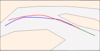
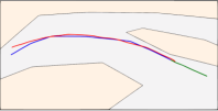
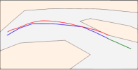
Line #2
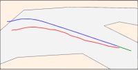
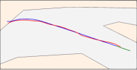
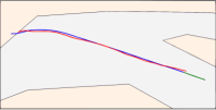
Line #3
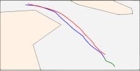
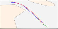
Line #4
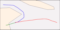
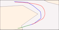
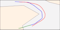
Line #5

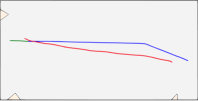
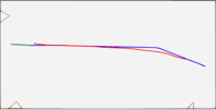
(a) Standard Features

(a) *

(b) Probabilistic Features

(b) *

(c) Trigonometrical Features

(c) *

Figure 10: Proposed Model with Convolutional Layers and Positional-Aware Attention (C1).
Legend: Green lines represent the input data, Blue the ground-truth, and Red the model forecasting.

Upon conducting a thorough examination of these various models, we can conclude that the complexity of the models varies based on the feature sets, vessel types, and individual model attributes. Nonetheless, despite these differences, the models consistently exhibited high-performance levels, with dissimilarities primarily arising from the preference for specific feature sets. Furthermore, our analysis unveiled a deeper facet of the models’ capabilities beyond the raw performance statistics. The models engage in intricate decision-making processes when working with diverse feature sets. For example, the increased standard deviation observed for trigonometric and probabilistic features does not necessarily indicate poor performance. Rather, it represents a unique form of dynamic decision-making that results in complex, erratic, yet precise trajectory shapes (i.e., routes) that may not be reflected in numerical consistency.

	[0.3][c]	[0.3][c]	[0.3][c]
Line #1
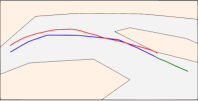
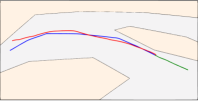
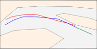
Line #2
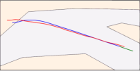
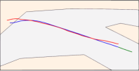
Line #3
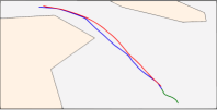
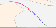
Line #4
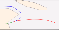
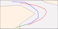
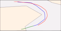
Line #5

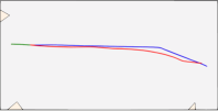
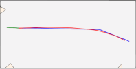
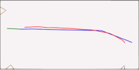
(a) Standard Features

(a) *

(b) Probabilistic Features

(b) *

(c) Trigonometrical Features

(c) *

Figure 11: Proposed Model with Convolutional Layers and without Positional-Aware Attention (C2).
Legend: Green lines represent the input data, Blue the ground-truth, and Red the model forecasting.

As further experiments, we designed and tested five different scenarios, which are illustrated in Figures 10, 11, 12, and 13. These scenarios aim to compare and validate the decision-making capability of different models and highlight that the evaluation metrics used for numerical analysis can be misleading in certain cases. Figure 10 shows the results for model C1, Figure 11 corresponds to C2, Figure 12 represents C3, while Figure 13 displays the model C4. As for model C5, we did not provide a visual representation due to its limited performance. However, the detailed results for this model are available in Tables 4 and 5.

	[0.3][c]	[0.3][c]	[0.3][c]
Line #1
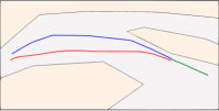
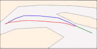
Line #2
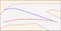
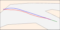
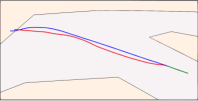
Line #3
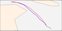
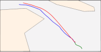
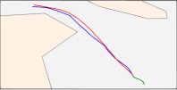
Line #4
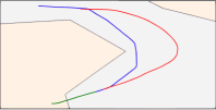
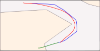
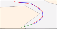
Line #5

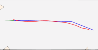
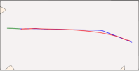
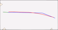
(a) Standard Features

(a) *

(b) Probabilistic Features

(b) *

(c) Trigonometrical Features

(c) *

Figure 12: Proposed Model without Convolutional Layers and with Positional-Aware Attention (C3).
Legend: Green lines represent the input data, Blue the ground-truth, and Red the model forecasting.

	[0.3][c]	[0.3][c]	[0.3][c]
Line #1
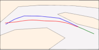
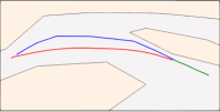
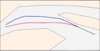
Line #2
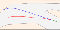
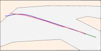
Line #3
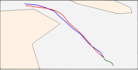
Line #4
Line #5

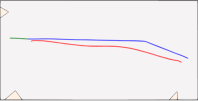
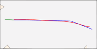
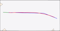
(a) Standard Features

(a) *

(b) Probabilistic Features

(b) *

(c) Trigonometrical Features

(c) *

Figure 13: Proposed Model without Convolutional Layers and Positional-Aware Attention (C4).
Legend: Green lines represent the input data, Blue the ground-truth, and Red the model forecasting.

In Figure 10, we can observe the performance of the proposed model (C1) on three sets of distinct features. The image highlights two incorrect path decisions made when using the Standard Features, which are images 2(a) and 4(a). Additionally, it shows poor forecasting performance in image 5(a). However, the other two feature sets exhibit perfect path decisions, with clear variations in the approximation of the forecasted path with the observed ones. In this case, the Trigonometrical Features are better suited for approximating the track in image 4(c) than the Probabilistic Features as seen in image 4(b). In contrast, the Probabilistic Features are better for image 4(b), albeit with a broader curve shape that increases the error.

In Figure 11, the proposed model is shown without the CNN layers (C2). It is evident that the lack of these layers for spatial feature extraction produces a more noisy approximation of several paths. Specifically, the 1(b)/1(c) and 2(b)/2(c) paths from the Probabilistic and Trigonometrical Features are poorly fitted. The previously well-fitted, curvy-shaped forecast for the Probabilistic Features is now loosely related to the input trajectory and the expected forecasting, as seen in image 4(b). On the other hand, the Trigonometrical Features show a better curve fitting in image 5(c), yet with highly imperfect forecastings due to the loss of spatial features sourced from the stacked convolutional layers. Moreover, the standard feature set still struggles to forecast the correct paths. Although there were minor improvements in images 1(a) and 5(a), the curvy-shaped 4(a) and the port-entering one 2(a) remain incorrect.

The image in Figure 12 shows a slight change in the setup, where there is no attention mechanism, but instead, the stack of convolution layers (C3) is used. The image also reveals that all three sets of features fail equally to fit images 1(a), 1(b), and 1(c). This suggests that the model might repeat a dominant pattern in the dataset, failing to account for changes in the features required to predict the correct trajectory. On the other hand, images 2(b) and 2(c), which depict a port entry, are correctly predicted for both Probabilistic and Trigonometrical features. However, for the standard feature set in image 2(a), it shows the worst result seen so far. Interestingly, the Trigonometrical Features are extremely well-fitted to the curvy-shape pattern, reasonably fitted by the Probabilistic Features, and somewhat fitted by the Standard Features, tracks shown in images 4(c), 4(b), and 4(a), respectively. This indicates that spatial patterns play a larger role in this set of experiments, but it can lead to an overfitting scenario as CNNs tend to repeat dominant patterns from the training dataset. In the complete model with all layers intact (C1), the attention mechanism functions as a filter for the spatial features, helping to control overfitting in the forecasting.

In Figure 13, the probabilistic features, as seen in image 4(b), perform better in curvy-shaped forecasting when compared to the trigonometrical features, as seen in image 4(c). However, all three feature sets fail to provide accurate information for the forecasting of images 1(a), 1(b), and 1(c). Similarly, the standard features fail to forecast images 2(a) and 4(a). Although image 5(a) moves in the correct direction, it fails to fit accurately as the other two sets of features managed to achieve in images 5(b) and 5(c).

Our set of experiments shows that the numerical variations in Tables 4 and 5 reflect the partial performance of the models in terms of long-term multi-path trajectory forecasting. Such discrepancy arises as the assessment metrics often fail to capture the inherent decision-making complexity of the deep-learning models, especially in scenarios involving predominantly linear trajectories. Even when the dataset is balanced and stratified, these metrics require additional inspection to fully appreciate the models’ ability to handle complex tasks. Moreover, the plethora of experiments has permitted us to identify the superior model for this study – model C1, trained on trigonometrical features. This model is proficient in accurately forecasting and visually representing all possible trajectories. In addition, the model performs better, yielding lower errors when trained on trigonometric features instead of probabilistic features. Therefore, the C1 model demonstrates superior path-decision capabilities, supported by the minimal approximation errors observed across the complete dataset of reserved vessels used for validation.

For a finer and more complete evaluation, in Figure 14, we show the results we achieved over the same test cases using the (a) Default Features with the TrAISformer model, the previous state-of-the-art on the task of long-term trajectory forecasting. Several adaptations were required to make the model suitable for the task we approach in this paper. Details about our adaptations to their model are available in the Methods. As can be observed in the images, the TrAISformer shows a similar performance to a simple sequence-to-sequence auto-encoder model when not trained with the probabilistic and trigonometric features. This means that their model, as is, is not capturing additional information that can help in the multi-path long-term trajectory forecasting problem. Besides this, TrAISformer has $7.6\times 10^{7}$ parameters, taking 1 hour and 30 minutes per training epoch and requiring 30 hours of training over the complete dataset. In contrast, the models tested and presented in the current paper are limited to $1.5\times 10^{7}$ parameters, five times fewer trainable parameters, in most cases requiring half a million trainable parameters, taking not more than 15 minutes per epoch and 3 hours to achieve a fully trained neural network. Details on the computational environment used for this experiment and computation can be found within the Methods.

Legend: Green lines represent the input data, Blue the ground-truth, and Red the model forecasting.

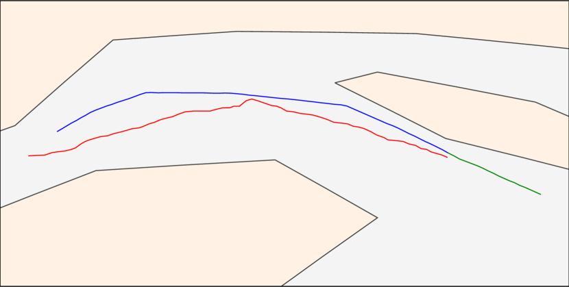
(a) Test case #1

(b) Test case #2

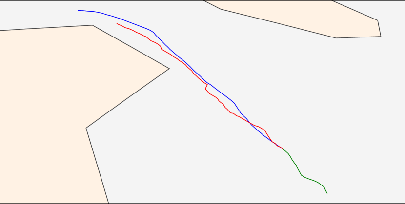
(c) Test case #3

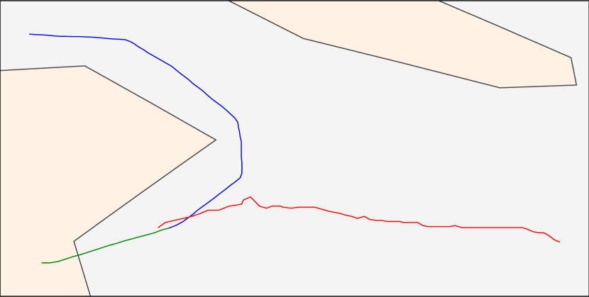
(d) Test case #4

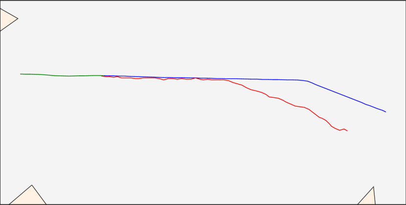
(e) Test case #5

Figure 14: TrAISformer [36] model over the five test cases using the (a) Default Features for comparison.

Table 6 presents the results obtained from the complete test dataset of cargo and tankers. Unlike the previous models, TrAISformer shows an $R^{2}$ result lower than the previously observed 98% for our proposed model. This is because the model was trained using teacher-forcing, which forecasts navigational metrics instead of approximating them using the trajectory coordinates. Therefore, the trajectories are geometrically noisy, even though some display correct direction and forecasted long-term paths. Based on the outcomes shown in Table 4 and 5, TrAISformer has achieved results similar to A1/C5 and B1/C5; they refer to simple unidirectional recurrent networks on an auto-encoder structure and do not rely on convolutional networks and the attention mechanism. Based on these results, we can conclude that utilizing probabilistic augmentation for trajectory data, such as AIS data, and employing different spatial projections for feature learning in auto-encoder sequence-to-sequence models achieves state-of-the-art results in long-term multi-path-trajectory forecasting. This approach proves to be the most effective strategy for handling uncertainty in open waters where there are multiple paths between origin and destination.

	$R^{2}$ Score	MAE	MSE	Mean Err.	25th Pct.	50th Pct.	75th Pct.	Std. Dev.
Tanker	96.67%	0.0966	0.0399	16.1471	3.6852	9.0399	19.9771	24.2283
Cargo	97.23%	0.0945	0.0342	15.6350	3.5165	8.7594	19.6720	21.4226

Table 6: Results from TrAISformer [36] over the entire dataset of Tanker and Cargo vessels.

Discussions

Our study highlights the significance of incorporating a probabilistic model within the trajectory forecasting process to enhance multi-path long-term vessel trajectory forecasting. During training, ground-truth data is used to construct transition probability matrices, providing the model with a nuanced perspective on potential vessel movements without the risk of overfitting. As the model is probabilistically driven, it stores motion statistics without relying heavily on the exact details of training data. This enables the model to distill a set of generalized patterns and rules from the data, which, while retaining a degree of uncertainty, does not compromise the model’s prediction capabilities. This controlled uncertainty enhances its ability to forecast under various conditions and adapt to the complexity of maritime navigation.

Our deep-learning model offers a unique advantage by combining exact coordinates from the Standard Features with conditional probabilities from the Probabilistic Features, allowing for a blend of precision and flexibility in predictive capabilities. This approach enables the model to identify intricate route patterns and make informed decisions that simpler baseline models often overlook. Through the Probabilistic Features, the model learns to navigate a domain where certainty is balanced with possibilities, reflecting real-world conditions where numerous factors can alter a vessel’s trajectory. This dynamic interplay between certainty and uncertainty makes the deep learning model more robust and less likely to fail.

The dual-model architecture with shared predictive responsibilities strengthens the overall system’s resilience, making it well-suited for real-time applications that process streaming AIS data. In this sense, our research contributes to trajectory forecasting by introducing a spatio-temporal model that integrates probabilistic feature engineering with deep learning techniques, significantly improving routing decisions on long-term vessel trajectory forecasting. We tested the model in various conditions with multiple feature sets and two vessel types, demonstrating its robustness and generalization in different contexts.

It is important to note that relying solely on numerical indicators can be misleading when deciding over complex scenarios. As we showed in the results, our model efficiently makes correct long-term path decisions, though it may only sometimes generate as straight paths as baseline models due to its noisiness. The ability of our model comes not only from the features but also the positional-aware attention mechanism in our deep-learning model, which significantly improves its ability to capture temporal dependencies, enabling it to learn nuanced temporal patterns that improve trajectory-fitting capabilities.

Furthermore, our study has practical implications concerning maritime safety and preserving biodiversity. Improved trajectory forecasting can significantly enhance navigational safety and prevent unintentional harm to marine life, particularly endangered species inhabiting busy sea routes such as the NARW. Our work inspires further research to improve the model’s performance, such as adding more route polygons across the Gulf of St. Lawrence and exploring techniques like Dynamic Time Warping as a loss function to reduce noise in generated trajectories. Furthermore, our model offers a foundation to harness the potential of sophisticated forecasting models, advancing maritime safety and proactively addressing ecological preservation concerns. In conclusion, our approach, combined with the efficient and flexible data processing capability of the Automatic Identification System Database (AISdb), sets a positive precedent for fostering reproducible research in vessel trajectory forecasting for the broader scientific community while harnessing the potential of deep learning and advancing maritime safety.

Methods

Dataset Description

Our dataset was collected from satellite-based Automatic Identification System (AIS) messages sent by vessels operating in the Gulf of St. Lawrence between 2015 and 2020. The AIS data was acquired from Spire, and it provides detailed records, including identification number, speed, location, vessel type, and timestamps. After cleaning the tracks, our final dataset consisted of 953 cargo and 391 tanker vessels for training, 51 cargo and 21 tanker vessels for validation, and 252 cargo and 103 tanker vessels for testing. The testing subset represents 20% of the entire dataset, while the validation subset (for deep-learning use) represents 20% of the non-testing data, and the outstanding data constitutes the training dataset.

Automatic Identification System Database (AISdb)

AISdb is a specialized platform developed to work with AIS data by the Marine Environmental Research Infrastructure for Data Integration and Application Network (MERIDIAN). AISdb is open-source software that offers a comprehensive toolkit for collecting and processing raw AIS data. It supports live streaming and historical raw AIS data files, making it a versatile solution for diverse requirements. AISdb’s core functionality relies on SQLite and Postgres databases, which can be used locally or remotely through a Python interface that enables querying, data processing, visualization, and curated data exportation.

AISdb is a powerful platform that provides an easy-to-use integration of AIS data with a wide range of environmental data stored in raster file formats. This integration is facilitated by the platform’s built-in functions, which allow users to download ocean bathymetric chart grids conveniently and query the depth of the sea floor beneath each surface vessel position. The platform is designed to accommodate raster data based on a longitude/latitude coordinate grid cell system, enabling users to merge various environmental data sources with AIS data. This provides a more comprehensive understanding of vessel movements and interactions with the marine environment, including temperature, salinity, and water quality. By offering such a wide range of features and capabilities, AISdb empowers users to conduct advanced research and analysis in the marine domain, which is ideal for academic and industrial use.

AISdb enables researchers to manage and utilize AIS data for their purpose, e.g., marine traffic risk mitigation, environmental studies, and marine surveillance, to name a few. Data can be requested as raw tracks or processed and extracted to a CSV file. This initiative is meant to benefit the research groups already involved in AIS-data research or those interested in engaging in it in the future. The availability of raw and unparsed data eliminates the need for preprocessing and preparing key data for various ocean-related AIS-driven tasks, thus making the research process more streamlined and efficient.

AISdb enables the reproducibility of AIS-related research, and due to its Python interface, it enables users to leverage machine and deep learning algorithms for vessel-task modeling. In such a sense, this research was made available in the AISdb platform, so any interested party can use AISdb to reproduce the results and scale up or down the research we have done using their own or our freely available data.

Algorithm 1 Calculate grid cell Probability

1:$C_{i}$ current grid cell of new track $\tau_{n}$; $S^{C_{i}}_{\tau_{n}}$ statistics of a new track $\tau_{n}\in C_{i}$; $k$ number of destinations;

2:function Possible-Destination($C_{i},S^{C_{i}}_{\tau_{n}},k$)

3:     $T_{C_{i}}=\left\{(S_{\tau}\rightarrow D_{j})|\tau_{C_{i}}=C_{i},\tau\in\widetilde{\mathbf{M}}\right\}$

4:     $C_{dest}=\left\{D_{j}|D_{j}\in T_{C_{i}}\right\}$

5:     $\mathbf{D}=\phi$

6:     for $(S_{\tau_{i}}\rightarrow D_{j})\in T_{C_{i}}$ do

7:         $dist=Euclidean(S_{\tau_{i}},S^{C_{i}}_{\tau_{n}})$

8:         $\mathbf{D}=\mathbf{D}\cup(D_{j},S_{\tau_{i}})\rightarrow dist$

9:     end for

10:     $CD=\phi$

11:     for $D_{i}\in C_{dest}$ do

12:         $D_{i}^{min}=min\left\{dist|dist\rightarrow\mathbf{D}(D_{j},S_{\tau}),D_{j}=D_{i}\right\}$

13:         $CD=CD\cup(D_{i}\rightarrow D_{i}^{min})$

14:     end for

15:     $\delta=\mu(\left\{D_{i}^{min}|(D_{i}\rightarrow D_{i}^{min})\in CD\right\})$

16:     $CD_{updated}=\phi$

17:     for $D_{i}\in C_{dest}$ do

18:         $D_{i}^{min}=D_{i}\in CD$

19:         if $D_{i}^{min}<\delta$  then

20:              $prob_{cx}=\frac{\left\|\left\{\tau|\tau\in T_{C_{i}},D_{j}\leftarrow\tau,D_{j}=D_{i}\right\}\right\|}{|T_{C_{i}}|}$

21:              $\mathsf{dist}_{i}=D_{i}^{min}\times(1-prob_{cx})$

22:              $CD_{updated}=CD_{updated}\cup(D_{i}\rightarrow\mathsf{dist}_{i})$

23:         end if

24:     end for

25:     return $\left\{f:D_{i}|(D_{i}\leftarrow\mathsf{dist}_{i})\in CD_{updated},\mathsf{dist}_{j}>\mathsf{dist}_{i},j\neq i,i=1,...,k\right\}$

26:end function

Estimation of Route and Destination

Our model for trajectory feature engineering is probabilistic. Its main objective is to predict the vessel’s most likely future location based on the current position, direction data, and historical AIS data. We require the ocean to be segmented into deterministic grids to achieve this. These grids integrate the movement patterns of various vessels over time based on their position data from historical AIS records. Each cell in the grid records when and how frequently vessels have visited that particular cell, storing their motion statistics along with it. The model operates on two levels. Firstly, it predicts the vessel’s route polygon along the trajectory. Secondly, it also predicts the most likely end-grid cell, which represents the completion of the vessel’s journey. Both are represented by their centroids, which are calculated separately for each AIS message in the vessel trajectory. The step-by-step procedure to find possible routes and destinations for a new trajectory ($\tau_{n}$) is provided in Algorithm 1, which requires as input: $C_{i}$, $S^{C_{i}}_{\tau_{n}}$, and $k$.

Herein, $C_{i}$ is the grid cell related to the current position of a vessel; $S^{C_{i}}_{\tau_{n}}$ is motion statistics of the new trajectory ($\tau_{n}$) in the grid cell $C_{i}$; lastly, $k$ represents the number of top probable destinations to consider. In Line 2, $T_{C_{i}}$ is a subset from $\widetilde{\mathbf{M}}$ (defined in Table 1) containing historical vessel motion statistics and destination related to grid cell $C_{i}$. We gather all unique possible destinations (end grid cell) $C_{dest}$ passing through $C_{i}$ in Line 3. In Line 4, we initialize the set $D$ as an empty set. Subsequently, we calculated the similarity between each historical track and the new trajectory in the current cell. The distance for each historical track (moving to a particular destination $D_{j}$) is stored in $D$. Lines 5–8 depicts the procedure where for each historical track’s statistics $S^{C_{i}}_{\tau_{i}}$, we calculate the Euclidean distance, labeled as $\mathsf{e}$, between $S_{\tau_{i}}$ and $S^{C_{i}}_{t_{n}}$. In the historical tracks, more than one track may pass through $C_{i}$ to a particular destination $D_{j}$. Thus, for each unique $D_{j}\in C_{dest}$, from all historical tracks that go to $D_{j}$, we consider only one track having the minimum distance $D_{i}^{min}$ (see Lines 10–13). The mean ($\mu$) of the population’s minimum distances in $CD$ is determined in Line 14. In $CD$, we only consider those destination $D_{j}$ whose distance is less than the mean $\delta$ — see Equation 4. Line 16-23 depicts the procedure to store the score in $CD_{updated}$. The score is calculated by multiplying the similarity score and probability tracking passing cell $C_{i}$ to reach a particular $D_{i}$. After processing, the function returns a set of tuples. Each tuple is uniquely identified by a pair of indices $(i,j)$, where $i\in[1,k]$ and $j$ denote the tuple’s rank.

TrAISformer Adaptations

As already mentioned, there are only a hand-full of models that are tailored for the long-term trajectory forecasting of AIS data due to the increased uncertainty in working on a large geographical environment over a long temporal range [62], making this problem very challenging to tackle and susceptible to many variables not intrinsically inherent to the positioning data provided by AIS messages. The prior state-of-the-art model [36] in such a task, for instance, was developed to classify instead of regress over data, adopting a space quantization strategy that also helps in reducing uncertainty and achieving better results. Such an approach adopts a sparse representation of AIS data and trains the transformer with multi-head attention. Due to our problem constraints, we were required to adapt their loss function as follows:

$$L_{total}=(\mathbb{L}_{lon}+\mathbb{L}_{lat}+\mathbb{L}_{v}+\mathbb{L}_{\theta}+\mathbb{L}_{\Delta_{v}}+\mathbb{L}_{\Delta_{\theta}})$$ (16)

The change was necessary because the original implementation of their model failed to converge over our dataset. In such cases, the loss function we adapt measures the variation within the prediction of each feature required by their model. This is a requirement because the authors are using teacher-forcing training, which is also the reason for the increased variability observed in the output results of their model. In our version of the loss function, $\mathbb{L}$ indicates the cross-entropy loss function applied over the quantized model-output results. A last modification for better performance and stability of their model over our dataset refers to masking the embedding using a left-padding strategy instead of a right-padding one to increase the model stability and match the input and output of the different models under testing.

Evaluation Metrics

When evaluating the performance of a probabilistic model, three metrics are used: Precision, Recall, and F1 Score. Precision measures the model’s ability to accurately identify only the relevant instances and is calculated by dividing true positive (TP) predictions by the sum of true positives and false positives (FP). Recall, also known as sensitivity, measures the model’s ability to identify all relevant instances and is calculated by dividing true positives by the sum of true positives and false negatives (FN). F1 Score is a performance assessment metric that combines both Precision and Recall, giving a more comprehensive evaluation of the model’s performance by taking the harmonic mean between these two values. To ensure a fair measure of model performance, each of these metrics is evaluated in a weighted manner.

$$\hfill Precision=\frac{TP}{TP+FP}\hfill$$ (17)

$$Recall=\frac{TP}{TP+FN}\hfill$$ (18)

$$\hfill F1\ Score=2\times\frac{{Precision\times Recall}}{{Precision+Recall}}\hfill$$ (19)

To evaluate the performance of our deep-learning model, we use: Mean Absolute Error – MAE, Mean Squared Error – MSE, and Coefficient of Determination – $R^{2}$. The MAE measures the average size of errors in a set of predictions. It is calculated as the average absolute differences between the predicted and actual observations. Each difference carries equal weight. The MAE is derived from the number of observations (n), the actual observations ($y_{i}$), and the predicted observations ($\hat{y}_{i}$). The MSE measures the average of the squares of the errors. It is a quality measure of an estimator, representing the average squared difference between the estimated values and the actual value. The MSE is always non-negative, and lower values are better. The $R^{2}$ score is a statistical measure that shows the proportion of the variance in a dependent variable explained by one or more independent variables in a regression model. It indicates the model’s goodness-of-fit and how well-unseen samples are likely to be predicted. The value of $R^{2}$ ranges from 0 to 1, where 1 indicates the linear regression fits the data perfectly, and 0 indicates that the average is a better predictor. In this case, $\bar{y}$ represents the mean of the observed data.

$$\hfill MAE=\frac{1}{n}\sum_{i=1}^{n}\left|y_{i}-\hat{y}_{i}\right|\hfill$$ (20)

$$\hfill MSE=\frac{1}{n}\sum_{i=1}^{n}\left(y_{i}-\hat{y}_{i}\right)^{2}\hfill$$ (21)

$$\hfill R^{2}=1-\frac{\sum_{i=1}^{n}\left(y_{i}-\hat{y}_{i}\right)^{2}}{\sum_{i=1}^{n}\left(y_{i}-\bar{y}\right)^{2}}\hfill$$ (22)

Speed

The speed of a vessel is given by the ratio of the distance between two points with respect to the time. The distance between two AIS messages (points) on the earth’s surface can be determined by the distance between the coordinates of $a,b\in\tau_{i}$ using the great circle distance. The Equation 23 takes into account the latitudes $\mathcal{L}_{at}^{a}$ and $\mathcal{L}_{at}^{b}$, the difference $\bigtriangleup^{\mathcal{L}_{on}}_{ab}$ between the longitudes $\mathcal{L}_{on}^{a}$ and $\mathcal{L}_{on}^{b}$, and the Earth’s radius $\mathbf{R}$ (6,371 km), values are given in radians.

$$\hfill\mathbb{D}(a,b)=\left(sin\left(\mathcal{L}_{at}^{a}\right)\times sin\left(\mathcal{L}_{at}^{b}\right)+cos\left(\mathcal{L}_{at}^{a}\right)\times cos\left(\mathcal{L}_{at}^{b}\right)\times cos\left({\bigtriangleup^{\mathcal{L}_{on}}_{qk}}\right)\times\mathbf{R}\right)\hfill$$ (23)

Using Equation 23, we calculate speed of a vessel to reach point $a$ from $b$:

$$\hfill v(b,a)=\frac{\mathbb{D}(a,b)}{(time_{b}-time_{a})}\hfill$$ (24)

Furthermore, the change in speed between locations is calculated as $\Delta_{v}=v_{2}-v_{1}$.

Bearing

The bearing is the direction of a vessel during its trajectory relative to the earth’s surface, calculated as:

$$\hfill\begin{aligned} \theta(a,b)\leavevmode\nobreak\ =\leavevmode\nobreak\ atan_{2}\Big{(}&sin\Big{(}\bigtriangleup_{\mathcal{L}_{on}}\Big{)}\times cos\Big{(}\mathcal{L}_{at}^{b}\Big{)},\\ &cos\Big{(}\mathcal{L}_{at}^{a}\Big{)}\times sin\Big{(}\mathcal{L}_{at}^{b}\Big{)}-sin\Big{(}\mathcal{L}_{at}^{a}\Big{)}\times cos\Big{(}\mathcal{L}_{at}^{b}\Big{)}\times cos\Big{(}\bigtriangleup_{\mathcal{L}_{on}}\Big{)}\Big{)}\end{aligned}\hfill$$ (25)

where $\bigtriangleup_{\mathcal{L}_{on}}$ is the difference between the longitudes of two points, $\Big{(}\mathcal{L}_{on}^{b}-\mathcal{L}_{on}^{a}\Big{)}$. Furthermore, the rate of bearing $\Delta_{\theta}$ is defined as the difference between two bearing values $\Big{(}\Delta_{\theta}=\theta_{2}-\theta_{1}\Big{)}$, adjusted to lie in the range of $[-180,180]$ by adding or subtracting 360 from $\Delta_{\theta}$ as needed.

Optimization Strategy

The optimization function we use encapsulates the strategy of independently minimizing the Mean Absolute Error (MAE) for both output components, latitude, and longitude, such as formalized below:

$$\hfill\min_{\Theta}\left(\frac{1}{N}\sum_{i=1}^{N}\left|\mathcal{L}_{at}^{i}-\widehat{\mathcal{L}_{at}^{i}}\right|+\frac{1}{N}\sum_{j=1}^{N}\left|\mathcal{L}_{on}^{j}-\widehat{\mathcal{L}_{on}^{j}}\right|\right)\hfill$$ (26)

Here, $y=\left<\mathcal{L}_{at},\mathcal{L}_{on}\right>$ symbolizes the original coordinates, and $\widehat{y}=\left<\widehat{\mathcal{L}_{at}},\widehat{\mathcal{L}_{on}}\right>$ symbolizes the predicted ones, while $\Theta$ stands as representation of the network parameters. For the optimization, we utilize the Adam optimizer with the learning rate of $1e^{-3}$ and weight decay of $1e^{-4}$ to prevent overfitting.

Model Hyperparameters

In order to ensure an unbiased evaluation, consistent hyperparameters were utilized across all experiments when constructing the deep learning model. L2 regularization was enforced with a regularization strength of 0.0005. Incremental convolutional blocks were employed with various numbers of filter sizes (256, 256, 128) and kernel sizes (7, 5, 5), with each block being subject to the stipulated L2 regularization. A Dropout Layer was added with a probability rate of 10%. The encoder-decoder architecture utilized bidirectional long- and short-term memory layers with 128 cells. Both the kernel and the recurrent weights in these layers used the ReLU activation function and L2 regularization. A Position-Aware Attention Mechanism was also incorporated to enhance the model’s attention to the input data’s temporal sequence. A time factor of 25% was employed for a balance between self-attention and the capturing of longer-term dependencies within the data sequence. Following the decoder, three dense layers were sequentially stacked. These layers had a decreasing number of neurons (128, 128, 64), and the ReLU function was activated for each.

Computing Environment

We conducted experiments on probabilistic and deep-learning models for trajectory forecasting in a high-performance computing environment. The environment was equipped with an NVIDIA A100 GPU GPU with 40GB of memory and 42 CPUs with 128GB of RAM running under Ubuntu 20.04 LTS.

Author contributions statement

Conceptualization, G.S., J.K.; methodology, G.S., J.K., R.P., and S.M.; AISdb software, G.S., J.K., M.S., S.V., R.G., R.P., and S.M.; validation, G.S., J.K., A.S., R.F., and D.E.; formal analysis, G.S.; data modeling, G.S., J.K., and D.E.; model optimization, G.S.; AISdb integration, G.S., J.K.; data curation, G.S., J.K., D.E., J.B., and T.F.; writing — original draft preparation, G.S. and J.K.; writing — review and editing, all authors; visualization, G.S. and J.K.; supervision, J.B., T.F., R.F., R.P., S.M.; project administration, G.S.; funding acquisition, G.S., R.P., S.M.; All authors have read and agreed to this version of the manuscript.

Competing interests

The authors declare no competing interests.

References

- [1] Organization, I. M. Brief history of imo. https://www.imo.org/en/About/HistoryOfIMO/Pages/Default.aspx. Accessed: 16th November 2023.
- [2] Organization, I. M. Ais transponders. https://www.imo.org/en/OurWork/Safety/Pages/AIS.aspx. Accessed: 16th November 2023.
- [3] Fournier, M., Casey Hilliard, R., Rezaee, S. & Pelot, R. Past, present, and future of the satellite-based automatic identification system: Areas of applications (2004–2016). \JournalTitleWMU journal of maritime affairs 17, 311–345 (2018).
- [4] Goerlandt, F. & Kujala, P. Traffic simulation based ship collision probability modeling. \JournalTitleReliability Engineering & System Safety 96, 91–107, DOI: 10.1016/j.ress.2010.09.003 (2011). Special Issue on Safecomp 2008.
- [5] Chen, P., Huang, Y., Mou, J. & van Gelder, P. Probabilistic risk analysis for ship-ship collision: State-of-the-art. \JournalTitleSafety Science 117, 108–122, DOI: 10.1016/j.ssci.2019.04.014 (2019).
- [6] Yang, D., Wu, L., Wang, S., Jia, H. & Li, K. X. How big data enriches maritime research–a critical review of automatic identification system (ais) data applications. \JournalTitleTransport Reviews 39, 755–773 (2019).
- [7] Harati-Mokhtari, A., Wall, A., Brooks, P. & Wang, J. Automatic identification system (ais): data reliability and human error implications. \JournalTitleThe Journal of Navigation 60, 373–389 (2007).
- [8] Millefiori, L. M. et al. Covid-19 impact on global maritime mobility. \JournalTitleScientific reports 11, 1–16 (2021).
- [9] Karataş, G. B., Karagoz, P. & Ayran, O. Trajectory pattern extraction and anomaly detection for maritime vessels. \JournalTitleInternet of Things 16, 100436 (2021).
- [10] Capobianco, S., Millefiori, L. M., Forti, N., Braca, P. & Willett, P. Deep learning methods for vessel trajectory prediction based on recurrent neural networks. \JournalTitleIEEE Transactions on Aerospace and Electronic Systems 57, 4329–4346 (2021).
- [11] Mustafa, H., Barrus, C., Leal, E. & Gruenwald, L. Gtraclus: A local trajectory clustering algorithm for gpus. In 2021 IEEE 37th International Conference on Data Engineering Workshops (ICDEW), 30–35 (IEEE, 2021).
- [12] Rong, H., Teixeira, A. & Soares, C. G. Data mining approach to shipping route characterization and anomaly detection based on ais data. \JournalTitleOcean Engineering 198, 106936 (2020).
- [13] Fu, P., Wang, H., Liu, K., Hu, X. & Zhang, H. Finding abnormal vessel trajectories using feature learning. \JournalTitleIEEE Access 5, 7898–7909 (2017).
- [14] Li, H. et al. Spatio-temporal vessel trajectory clustering based on data mapping and density. \JournalTitleIEEE Access 6, 58939–58954 (2018).
- [15] Haranwala, Y. J., Spadon, G., Renso, C. & Soares, A. A data augmentation algorithm for trajectory data. In 1st ACM SIGSPATIAL International Workshop on Methods for Enriched Mobility Data: Emerging issues and Ethical perspectives 2023 (EMODE ’23), 5, DOI: 10.1145/3615885.3628008 (ACM, New York, NY, USA, New York, NY, USA, 2023).
- [16] Wang, C., Ren, H. & Li, H. Vessel trajectory prediction based on ais data and bidirectional gru. In 2020 International Conference on Computer Vision, Image and Deep Learning (CVIDL), 260–264 (IEEE, 2020).
- [17] Park, J., Jeong, J. & Park, Y. Ship trajectory prediction based on bi-lstm using spectral-clustered ais data. \JournalTitleJournal of Marine Science and Engineering 9, 1037 (2021).
- [18] Murray, B. & Perera, L. P. A dual linear autoencoder approach for vessel trajectory prediction using historical ais data. \JournalTitleOcean Engineering 209, 107478, DOI: 10.1016/j.oceaneng.2020.107478 (2020).
- [19] Campbell, J. N., Isenor, A. W. & Ferreira, M. D. Detection of invalid ais messages using machine learning techniques. \JournalTitleProcedia Computer Science 205, 229–238 (2022).
- [20] Spadon, G., Ferreira, M. D., Soares, A. & Matwin, S. Unfolding ais transmission behavior for vessel movement modeling on noisy data leveraging machine learning. \JournalTitleIEEE Access (2022).
- [21] Peng, Z. et al. Establishment of inland ship air pollution emission inventory based on power method correction model. \JournalTitleSustainability 14, 11188 (2022).
- [22] Pichegru, L. et al. Maritime traffic trends around the southern tip of africa–did marine noise pollution contribute to the local penguins’ collapse? \JournalTitleScience of The Total Environment 849, 157878 (2022).
- [23] Nguyen, D., Vadaine, R., Hajduch, G., Garello, R. & Fablet, R. A multi-task deep learning architecture for maritime surveillance using ais data streams. In 2018 IEEE 5th International Conference on Data Science and Advanced Analytics (DSAA), 331–340 (IEEE, 2018).
- [24] Patmanidis, S., Voulgaris, I., Sarri, E., Papavassilopoulos, G. & Papavasileiou, G. Maritime surveillance, vessel route estimation and alerts using ais data. In 2016 24th Mediterranean Conference on Control and Automation (MED), 809–813 (IEEE, 2016).
- [25] Zhang, Y.-l., Peng, P.-f., Liu, J.-s. & Liu, S.-k. Ais data oriented ships’ trajectory mining and forecasting based on trajectory delimiter. In 2018 10th International Conference on Intelligent Human-Machine Systems and Cybernetics (IHMSC), vol. 1, 269–273 (IEEE, 2018).
- [26] Üney, M., Millefiori, L. M. & Braca, P. Data driven vessel trajectory forecasting using stochastic generative models. In IEEE International Conference on Acoustics, Speech and Signal Processing (ICASSP), 8459–8463 (IEEE, 2019).
- [27] Faghih-Roohi, S., Xie, M. & Ng, K. M. Accident risk assessment in marine transportation via markov modeling and markov chain monte carlo simulation. \JournalTitleOcean engineering 91, 363–370 (2014).
- [28] Le Guillarme, N. & Lerouvreur, X. Unsupervised extraction of knowledge from s-ais data for maritime situational awareness. In Proceedings of the 16th International Conference on Information Fusion, 2025–2032 (IEEE, 2013).
- [29] d’Afflisio, E., Braca, P., Millefiori, L. M. & Willett, P. Maritime anomaly detection based on mean-reverting stochastic processes applied to a real-world scenario. In 2018 21st International Conference on Information Fusion (FUSION), 1171–1177 (IEEE, 2018).
- [30] Forti, N., Millefiori, L. M. & Braca, P. Unsupervised extraction of maritime patterns of life from automatic identification system data. In OCEANS 2019-Marseille, 1–5 (IEEE, 2019).
- [31] Forti, N., Millefiori, L. M., Braca, P. & Willett, P. Anomaly detection and tracking based on mean–reverting processes with unknown parameters. In ICASSP 2019-2019 IEEE International Conference on Acoustics, Speech and Signal Processing (ICASSP), 8449–8453 (IEEE, 2019).
- [32] Ferreira, M. D., Spadon, G., Soares, A. & Matwin, S. A semi-supervised methodology for fishing activity detection using the geometry behind the trajectory of multiple vessels. \JournalTitleSensors 22, 6063 (2022).
- [33] Newaliya, N. & Singh, Y. A review of maritime spatio-temporal data analytics. In 2021 International Conference on Computational Performance Evaluation (ComPE), 219–226 (IEEE, 2021).
- [34] Xiao, Z., Fu, X., Zhang, L. & Goh, R. S. M. Traffic pattern mining and forecasting technologies in maritime traffic service networks: A comprehensive survey. \JournalTitleIEEE Transactions on Intelligent Transportation Systems 21, 1796–1825, DOI: 10.1109/TITS.2019.2908191 (2020).
- [35] Pallotta, G., Horn, S., Braca, P. & Bryan, K. Context-enhanced vessel prediction based on ornstein-uhlenbeck processes using historical ais traffic patterns: Real-world experimental results. In 17th international conference on information fusion (FUSION), 1–7 (IEEE, 2014).
- [36] Nguyen, D. & Fablet, R. A transformer network with sparse augmented data representation and cross entropy loss for ais-based vessel trajectory prediction. \JournalTitleIEEE Access 1–1, DOI: 10.1109/ACCESS.2024.3349957 (2024).
- [37] Nguyen, D. & Fablet, R. TrAISformer-a generative transformer for AIS trajectory prediction. \JournalTitleCoRR abs/2109.03958 (2021). 2109.03958.
- [38] Lamb, A. M. et al. Professor forcing: A new algorithm for training recurrent networks. In Lee, D., Sugiyama, M., Luxburg, U., Guyon, I. & Garnett, R. (eds.) Advances in Neural Information Processing Systems, vol. 29 (Curran Associates, Inc., 2016).
- [39] Capobianco, S., Millefiori, L. M., Forti, N., Braca, P. & Willett, P. Deep learning methods for vessel trajectory prediction based on recurrent neural networks. \JournalTitleIEEETransactions on Aerospace and Electronic Systems 57, 4329–4346, DOI: 10.1109/TAES.2021.3096873 (2021).
- [40] Capobianco, S., Forti, N., Millefiori, L. M., Braca, P. & Willett, P. Recurrent encoder-decoder networks for vessel trajectory prediction with uncertainty estimation. \JournalTitleIEEE Transactions on Aerospace and Electronic Systems 1–12, DOI: 10.1109/TAES.2022.3216823 (2022).
- [41] O’Brien, O. et al. Repatriation of a historical north atlantic right whale habitat during an era of rapid climate change. \JournalTitleScientific Reports 12, 1–10 (2022).
- [42] Davies, K. T. & Brillant, S. W. Mass human-caused mortality spurs federal action to protect endangered north atlantic right whales in canada. \JournalTitleMarine Policy 104, 157–162 (2019).
- [43] Spadon, G., Carvalho, A. C. d., Rodrigues-Jr, J. F. & Alves, L. G. Reconstructing commuters network using machine learning and urban indicators. \JournalTitleScientific reports 9, 11801 (2019).
- [44] Lei, W., Alves, L. G. & Amaral, L. A. N. Forecasting the evolution of fast-changing transportation networks using machine learning. \JournalTitleNature communications 13, 4252 (2022).
- [45] Alves, L. G., Rybski, D. & Ribeiro, H. V. Commuting network effect on urban wealth scaling. \JournalTitleScientific Reports 11, 22918 (2021).
- [46] Rodrigues-Jr, J. F., Gutierrez, M. A., Spadon, G., Brandoli, B. & Amer-Yahia, S. Lig-doctor: Efficient patient trajectory prediction using bidirectional minimal gated-recurrent networks. \JournalTitleInformation Sciences 545, 813–827, DOI: 10.1016/j.ins.2020.09.024 (2021).
- [47] Rodrigues-Jr, J. F., Spadon, G., Brandoli, B. & Amer-Yahia, S. Patient trajectory prediction in the mimic-iii dataset, challenges and pitfalls. \JournalTitleCoRR abs/1909.04605 (2019). 1909.04605.
- [48] Spadon, G. et al. Pay attention to evolution: Time series forecasting with deep graph-evolution learning. \JournalTitleIEEE Transactions on Pattern Analysis and Machine Intelligence 44, 5368–5384, DOI: 10.1109/TPAMI.2021.3076155 (2022).
- [49] Spadon, G. et al. Behavioral characterization of criminality spread in cities. In International Conference on Computational Science (ICCS), vol. 108, 2537–2541, DOI: 10.1016/J.PROCS.2017.05.118 (Elsevier, 2017).
- [50] Spadon, G., Gimenes, G. & Rodrigues-Jr, J. F. Identifying urban inconsistencies via street networks. \JournalTitleProcedia Computer Science 108, 18–27, DOI: 10.1016/j.procs.2017.05.103 (2017). International Conference on Computational Science, ICCS 2017, 12-14 June 2017, Zurich, Switzerland.
- [51] Spadon, G., Gimenes, G. & Rodrigues, J. F. Topological street-network characterization through feature-vector and cluster analysis. In Computational Science – ICCS 2018: 18th International Conference, Wuxi, China, June 11–13, 2018, Proceedings, Part I, 274–287, DOI: 10.1007/978-3-319-93698-7_21 (Springer-Verlag, Berlin, Heidelberg, 2018).
- [52] Spadon, G., Brandoli, B., Eler, D. M. & Rodrigues-Jr, J. F. Detecting multi-scale distance-based inconsistencies in cities through complex-networks. \JournalTitleJournal of Computational Science 30, 209–222, DOI: 10.1016/j.jocs.2018.12.015 (2019).
- [53] Huang Tang, Y. Y. & Shen, H. A model for vessel trajectory prediction based on long short-term memory neural network. \JournalTitleJournal of Marine Engineering & Technology 21, 136–145, DOI: 10.1080/20464177.2019.1665258 (2022).
- [54] Suo, Y., Chen, W., Claramunt, C. & Yang, S. A ship trajectory prediction framework based on a recurrent neural network. \JournalTitleSensors 20, DOI: 10.3390/s20185133 (2020).
- [55] Ibadurrahman et al. Long-term ship position prediction using automatic identification system (ais) data and end-to-end deep learning. \JournalTitleSensors 21, DOI: 10.3390/s21217169 (2021).
- [56] Gao, M., Shi, G. & Li, S. Online prediction of ship behavior with automatic identification system sensor data using bidirectional long short-term memory recurrent neural network. \JournalTitleSensors 18, DOI: 10.3390/s18124211 (2018).
- [57] Bao, K. et al. An improved ship trajectory prediction based on ais data using mha-bigru. \JournalTitleJournal of Marine Science and Engineering 10, DOI: 10.3390/jmse10060804 (2022).
- [58] Yang, C.-H., Wu, C.-H., Shao, J.-C., Wang, Y.-C. & Hsieh, C.-M. Ais-based intelligent vessel trajectory prediction using bi-lstm. \JournalTitleIEEE Access 10, 24302–24315, DOI: 10.1109/ACCESS.2022.3154812 (2022).
- [59] Murray, B. & Perera, L. P. An ais-based deep learning framework for regional ship behavior prediction. \JournalTitleReliability Engineering & System Safety 215, 107819, DOI: 10.1016/j.ress.2021.107819 (2021).
- [60] Liu, T. & Ma, J. Ship navigation behavior prediction based on ais data. \JournalTitleIEEE Access 10, 47997–48008, DOI: 10.1109/ACCESS.2022.3172308 (2022).
- [61] Capobianco, S., Forti, N., Millefiori, L. M., Braca, P. & Willett, P. Uncertainty-aware recurrent encoder-decoder networks for vessel trajectory prediction. In 2021 IEEE 24th International Conference on Information Fusion (FUSION), 1–5, DOI: 10.23919/FUSION49465.2021.9626839 (2021).
- [62] Zhang, X., Fu, X., Xiao, Z., Xu, H. & Qin, Z. Vessel trajectory prediction in maritime transportation: Current approaches and beyond. \JournalTitleIEEE Transactions on Intelligent Transportation Systems 23, 19980–19998, DOI: 10.1109/TITS.2022.3192574 (2022).
Acknowledgments
This research received partial funding from several organizations, including the Natural Sciences and Engineering Research Council of Canada (NSERC) through grant number RGPIN-2022-03909, the Institute for Big Data Analytics (IBDA), and the Ocean Frontier Institute (OFI) at Dalhousie University in Halifax, NS, Canada. The research was also supported by the São Paulo Research Foundation (FAPESP) through grants #2016/17078-0 and #2022/12374-1. Additionally, it received further funding from the Canada First Research Excellence Fund (CFREF) and the Canadian Foundation for Innovation’s MERIDIAN cyberinfrastructure. We thank all funding sources and Spire for providing the vessel track dataset.