The intrinsic geometry determined by the Cauchy problems of the Camassa-Holm equation

Abstract

Pseudospherical surfaces determined by Cauchy problems involving the Camassa-Holm equation are considered herein. We study how global solutions influence the corresponding surface, as well as we investigate two sorts of singularities of the metric: the first one is just when the co-frame of dual form is not linearly independent. The second sort of singularity is that arising from solutions blowing up. In particular, it is shown taht the metric blows up if and only if the solution breaks in finite time.

MSC classification 2020: 35A01, 74G25, 37K40 , 35Q51.

Keywords Equations describing pseudospherical surfaces  $\cdot$ Geometric analysis  $\cdot$ Existence of metrics  $\cdot$ Blow up of metrics

1 Introduction

Chern and Tenenblat introduced the notion of pseudospherical equations [10], connecting certain special partial differential equations (PDEs) with infinitely differentiable two-dimensional Riemannian manifolds. Roughly speaking, an equation is said to describe a pseudospherical surface (PSS equation) if it is a necessary and sufficient condition for the validity of the structure equations determining a surface of Gaussian curvature ${\cal K}=-1$. As a result, solutions of such an equation determines a co-frame for a pseudospherical metric of a pseudospherical surface (PSS) with ${\cal K}=-1$. This concept will be accordingly and timely revisited in the present work.

One of the most well-known equations of this type is the third order equation

$$u_{t}-u_{txx}+3uu_{x}=2u_{x}u_{xx}+uu_{xxx},$$ (1.0.1)

that was deduced by Camassa and Holm [6] as a shallow water model, named after them, and shown to be a PSS equation by Reyes [56]. Amongst a number of features the Camassa-Holm (CH) equation has, we would like to highlight existence of differentiable, but not smooth, solutions breaking at finite time [13]. Throughout this paper, by smooth we mean $C^{\infty}$.

Subsequent developments and applications of Chern and Tenenblat’s ideas have not considered solutions with initial data nor finite regularity. As a result, the solutions examined in [13] are, at first sight, somewhat incompatible with the theory developed in [10]. This incongruity might, and probably does, explain the lack of studies of PSS determined by solutions of the Camassa-Holm equation with finite regularity. Very likely, this is the root of a more general fact, that is the absence of works considering surfaces determined by Cauchy problems involving PSS equations.

Only very recently some light have been shed on problems of the nature mentioned above. In [62] qualitative properties of PSS determined by a certain equation reported in [28], (but discovered in a different context in [52]), was studied in conjunction with Cauchy problems. Despite its innovative approach, such a connection was made by considering smooth solutions.

A step forward was made soon after, in [22], where PSS surfaces determined by periodic Cauchy problems involving the equation studied in [62, 28] was considered. This led the authors to prove the existence of periodic PSS and, more importantly, for the first time a finite regularity geometric problem was considered.

Papers [22, 62] are pioneering studies of PSS in connection with Cauchy problems. However, in view of the qualitative nature of the solutions of the Cauchy problems involved, no solution developing any sort of singularities were considered.

A significant leap has been made in [31], where blowing up solutions of the CH were shown to determined PSS. It was proved that the corresponding metric of the surface can only exist within a strip of finite height in the $(x,t)$ plane and also experiences a blow up. Indeed, perhaps the most remarkable result proved in [31] is that any non-trivial initial datum in a certain Sobolev class will necessarily define a co-frame for a pseudospherical metric for a PSS.

The progress made in [31] would not be possible at no cost: A sine qua non ingredient that enabled the advances carried out in [31] was the reformulation of the notions of PSS determined by an equation and generic solutions.

Despite the significant findings reported in [31], some relevant points remain unclear: in the literature of the CH equation, there are blow up scenarios other than those considered in [31], but we had no more than clues about if they really could always be transferred to the metric and that being so, how that happens. From a completely different nature, not to say opposite, the results reported in [31] showed that any non-trivial initial datum defines a strip contained on the upper plane where a co-frame can be defined everywhere, but it remains unclear if or when we could extend the strip to the entire upper plane.

1.1 Novelty of the manuscript

While the results reported in [31] showed that any non-trivial initial datum gives rise to a PSS whose dual co-frame is defined on a strip of height $T>0$, they left many open questions. For example, the blow up mechanisms explored in that reference are not the only ones leading to a breakdown of the solutions. In addition, no attempt has been made to consider the possibility of having $T=\infty$, nor problems concerning how persistence properties of the solutions may affect the corresponding PSS.

This paper shows that we may have PSS defined on subsets of arbitrary height. Moreover, we additionaly study PSS determined by compactly supported initial conditions, precisely describing the asymptotic behaviour of the metric. Furthermore, other blow up conditions for the metrics are also predicted. More importantly, we prove that the metric blows up if and only if the solution develops wave breaking.

1.2 Outline of the manuscript

In section 2 we revisit some basic and relevant aspects of the CH equation, with main focus on the two-dimensional Riemannian geometry determined by its solutions and open problems regarding its geometric analysis. Next, in section 3 we fix the notation used throughout the manuscript, recall basic notions and state our main results. In section 4 we revisit some useful facts, such as conserved quantities and qualitative results regarding the CH equation, that are widely employed in section 5, where our main results are proved. In section 6 we show that the metric of the surface blows up if and only if the solution breaks in finite time. Some examples illustrating our main results are discussed in section 7, while our discussions and conclusions are presented in sections 8 and 9, respectively.

2 Few facts about the CH equation and the geometry determined by its solutions

Despite being primarily deduced as an approximation for the description of waves propagating in shallow water regimes, the equation proved to have several interesting properties related to integrability [6]. If we denote

$$m(x,t):=u(x,t)-u_{xx}(x,t),$$

which is known as momentum [6], then (1.0.1) can be rewritten as an evolution equation for $m$, namely,

$$m_{t}+2u_{x}m+um_{x}=0.$$ (2.0.1)

It was shown in [6] that (2.0.1) has a bi-Hamiltonian structure, having the representations

$$m_{t}=-{\cal B}_{1}\frac{\delta{\cal H}_{2}}{\delta m}=-{\cal B}_{2}\frac{\delta{\cal H}_{1}}{\delta m},$$

where

$${\cal B}_{1}(\cdot)=\partial_{x}(1-\partial_{x}^{2})(\cdot),\quad{\cal B}_{2}(\cdot)=\partial_{x}(m\cdot)+m\partial_{x}(\cdot)$$

are the Hamiltonian operators, and the functionals ${\cal H}_{1}$ and ${\cal H}_{2}$ are

$${\cal H}_{1}=\frac{1}{2}\int_{\mathbb{R}}(u^{2}+u_{x}^{2})dx,\quad{\cal H}_{2}=\frac{1}{2}\int_{\mathbb{R}}(u^{3}+uu_{x}^{2})dx.$$ (2.0.2)

As a consequence of its bi-Hamiltonian structure, (2.0.1) has also a recursion operator ${\cal R}={\cal B}_{2}{\cal B}_{1}^{-1}$ and infinitely many symmetries as well, being also integrable in this sense. The reader is referred to [54, Chapter 7] or [53] for further details about recursion operators and integrability.

It is still worth of mention that Camassa and Holm showed a Lax formulation [6] for (1.0.1)

$$\psi_{xx}=\displaystyle{\Big{(}\frac{1}{4}-\frac{m}{2\lambda}\Big{)}\psi},\,\,\,\,\psi_{t}=\displaystyle{-(\lambda+u)\psi_{x}+\frac{1}{2}u_{x}\psi}$$ (2.0.3)

as well as continuous, piecewise soliton like solutions, called peakons. For a review on the Camassa-Holm and related equations, see [25].

2.1 Wave breaking of solutions

Soon after the seminal work [6], the interest and relevance of the equation spread out the field of integrable equations and arrived at the lands of applied analysis. Solutions emanating from Cauchy problems involving initial data in certain Banach spaces were proved to be locally well-posed, being global under additional conditions [12]. Even more interestingly, depending on the slope of the initial datum there exists a finite value $T>0$ (the lifespan of the solution), such that

$$\liminf_{t\rightarrow T}\big{(}\inf_{x\in\mathbb{R}}u_{x}(x,t)\big{)}=-\infty.$$ (2.1.1)

This fact was first observed in [6] and its rigorous demonstration and dependence on the initial datum was shown by Constantin and Escher [13], see also the review [23].

The Hamiltonian ${\cal H}_{1}$ in (2.0.2) is equivalent to the square of the Sobolev $H^{1}(\mathbb{R})-$norm of the solution, meaning that solutions with enough decaying at infinity (as those emanating from initial data $u_{0}\in H^{s}(\mathbb{R})$, $s>3/2$) remain uniformly bounded by the norm of the initial datum as long as they exist [12, 23, 60].

On the other hand, (2.1.1) says that the first singularity (blow up) of a solution, whether it occurs, is manifested by the non-existence of any lower bound of $u_{x}$ as $t$ approaches a finite time $T$, at least for some point $x\in\mathbb{R}$ [13, Theorem 4.2]. The sudden steepening shown in (2.1.1), but preserving the shape of the solution, is better known as wave breaking (of $u$).

2.2 Geometric aspects of the CH equation

The Camassa-Holm (CH) equation, or its solutions, can also be studied from geometric perspectives [14, 15, 16, 56]. We shall briefly discuss [14, 56] which are the main inspirations for this paper, the first being concerned with infinite dimensional Riemmanian geometry, whereas the latter is concerned with an abstract two-dimensional Riemannian manifold, whose importance for this paper is crucial.

Equation (1.0.1) can be associated with the geometric flow in an infinite dimensional manifold ${\cal D}^{3}(\mathbb{R})$ modelled by a Hilbert space in which we can endow a (weak) Riemannian metric [14]. The geodesics in ${\cal D}^{3}(\mathbb{R})$ can either exist globally [14, Theorem 6.1] or breakdown in finite time [14, Theorems 6.3 and 6.4] and, in particular, geodesics starting, at the identity, with initial velocity corresponding to initial datum leading to breaking solutions will also develop singularities at finite time [14, Theorem 6.3].

A different geometric perspective for the CH equation was given by Reyes [56], who showed it describes pseudospherical surfaces [56, Theorem 1] à la Chern and Tenenblat [10], e.g. see [7, Definition 2.1].

Definition 2.1.

A pseudospherical surface $(PSS)$ is a two-dimensional Riemannian manifold whose Gaussian curvature is constant and negative.

For now it suffices saying that an equation describes pseudospherical surfaces, or is of the pseudospherical type, henceforth referred as PSS equation, when the equation is the compatibility condition of the structure equations

$$d\omega_{1}=\omega_{3}\wedge\omega_{2},\quad d\omega_{2}=\omega_{1}\wedge\omega_{3},\quad d\omega_{3}=-{\cal K}\omega_{1}\wedge\omega_{2},$$ (2.2.1)

for a PSS.

That said, in section 2 we show how from a given solution of the CH equation we can construct intrinsically a two-dimensional manifold having Gaussian curvature ${\cal K}=-1$.

The impossibility of a complete realisation of these surfaces in the three-dimensional space is a consequence of Hilbert theorem, which states one cannot immerse isometrically a complete surface with negative curvature into $\mathbb{R}^{3}$ [51, page 439], [46]. See also [21, section 5-11] for a proof of the Hilbert theorem. This explains the adjective abstract often used to qualify a PSS.

In his work Reyes showed that if $u$ is a solution of the CH equation, $m$ is its corresponding momentum, then the one-forms

$$\begin{array}[]{lcl}\omega_{1}&=&\displaystyle{\Big{(}\frac{\lambda}{2}+\frac{1}{2\lambda}-m\Big{)}dx+\Big{(}um+\frac{\lambda}{2}u-\frac{u}{2\lambda}-\frac{1}{2}-\frac{\lambda^{2}}{2}\Big{)}dt},\\ \\ \omega_{2}&=&-u_{x}dt,\\ \\ \omega_{3}&=&\displaystyle{\Big{(}m+\frac{1}{2\lambda}-\frac{\lambda}{2}\Big{)}dx+\Big{(}\frac{\lambda^{2}}{2}-\frac{1}{2}-\frac{u}{2\lambda}-\frac{\lambda}{2}u-um\Big{)}dt},\end{array}$$ (2.2.2)

satisfy (2.2.1), for any $\lambda\in\mathbb{R}\setminus\{0\}$ and ${\cal K}=-1$. This implies that the domain of the solution $u$, under certain circumstances, can be endowed with a Riemannian metric $g=\omega_{1}^{2}+\omega_{2}^{2}$ of a PSS, also known as first fundamental form of the surface. From (2.2.2), the corresponding metric is

$$\begin{array}[]{lcl}g&=&\displaystyle{\Big{(}\frac{\lambda}{2}+\frac{1}{2\lambda}-m\Big{)}^{2}dx^{2}}+\displaystyle{2\Big{(}\frac{\lambda}{2}+\frac{1}{2\lambda}-m\Big{)}\Big{(}um+\frac{\lambda}{2}u-\frac{u}{2\lambda}-\frac{1}{2}-\frac{\lambda^{2}}{2}\Big{)}dxdt}\\ \\ &+&\displaystyle{\Big{[}u_{x}^{2}+\Big{(}um+\frac{\lambda}{2}u-\frac{u}{2\lambda}-\frac{1}{2}-\frac{\lambda^{2}}{2}\Big{)}^{2}}\Big{]}dt^{2}=:\displaystyle{g_{11}dx^{2}+2g_{12}dxdt+g_{22}dt^{2}}.\end{array}$$ (2.2.3)

More precisely, the work of Reyes showed that, in fact, the Camassa-Holm equation is geometrically integrable, in the sense that its solutions may describe a one-parameter family of non-trivial pseudospherical surfaces [56, Corollary 1]. This is a reflection that the parameter $\lambda$ in (2.2.2) cannot be removed under a gauge transformation

While in [14] the influence of solutions emanating from Cauchy problems is crucial in the study of the existence and formation of singularities of geodesics, this is a point usually not considered in the literature of PSS equations, see [8, 9, 17, 18, 10, 20, 22, 39, 40, 41, 55, 56, 57, 58, 59, 63] and references therein. Moreover, in the study of PSS and PDEs the solutions are assumed to be smooth, very often implicitly, but sometimes clearly mentioned [8, page 2] and [41, page 2].

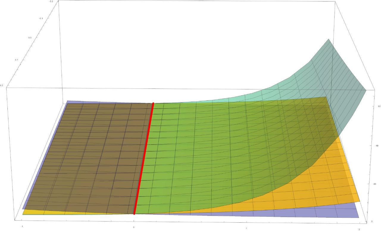
Figure 1: Graphs of solutions $u(x,t)=e^{x-ct}$ of the CH equation for different values of $c$. The curve $x\mapsto(x,0,e^{x})$, highlighted in red, belongs to the graph of this function for any value of $c$.

A smooth solution of a PSS equation leads to smooth one-forms $\omega_{1},\omega_{2},\omega_{3}$ and then the corresponding first fundamental form will inherit the same regularity. The solutions considered by Constantin [14], on the contrary, are not necessarily $C^{\infty}$, showing an enormous difference among [14] and [8, 7, 55, 56, 57, 58, 59, 63] in terms of the regularity of the objects considered.

Additionally, in the context of the literature of PDEs and PSS, the problem of uniqueness of solutions is not usually discussed, then the question of whether a given first fundamental form could be associated to one or more solutions of the CH equation has not been yet considered. Therefore, a situation like the one shown in Figure 1 is very likely to happen: how can one study the intrinsic geometry associated to the solutions of the CH equation when our only information is a known curve on the boundary of its graph?

3 Notation, notions and main results

Throughout this paper $u=u(x,t)$ denotes a function depending on the variables $x$ and $t$, whose physical meaning, when considering the model (1.0.1), are height of the free surface of water above a flat bottom, space and time, respectively. From a geometric point of view, $x$ and $t$ are coordinates of a domain in $\mathbb{R}^{2}$ in which the function $u$ is defined. We denote by $u(x,\cdot)$ and $u(\cdot,t)$ the functions $t\mapsto u(x,t)$, for fixed $x$, and $x\mapsto u(x,t)$, for fixed $t$, respectively.

For given two non-empty and connected subsets $I,J\subseteq\mathbb{R}$, the notation $u\in C^{0}(I\times J)$ means that $u=u(x,t)$ is continuous with respect to both variables in $I\times J$. By $u_{x}$ or $\partial_{x}u$ we denote partial derivative of $u$ with respect to its first argument, while similarly $u_{t}$ or $\partial_{t}u$ will denote partial derivative with respect to the second argument. We can also consider higher order derivatives using similar convention.

The set of ordered $n-th$ derivatives of $u$, $n\in{\mathbb{N}}$, is denoted by $u_{(n)}$. By convention, $u_{(0)}=u$. Whenever $u$ and its all derivatives up to order $k\in{\mathbb{N}}\cup\{0\}$ are continuous on the domain of $u$, we then write $u\in C^{k}$. The sets of smooth functions defined on a domain $\Omega\subseteq\mathbb{R}^{2}$ is denoted by $C^{\infty}(\Omega)$.

Given $n\in{\mathbb{N}}$, a non-empty set $I\subseteq\mathbb{R}$ and a Banach space $X$, we say that $u\in C^{n}(X,I)$ whenever $\partial_{x}^{k}u(\cdot,t)\in C^{0}(X,I)$, $0\leq k\leq n$. Moreover, $u\in C^{0}(X,I)$ means $u(\cdot,t)\in X$ and $\|u\|_{C^{0}}=\sup_{t\in I}\|u(\cdot,t)\|_{X}$.

3.1 Sobolev spaces

The Sobolev spaces $H^{s}(\mathbb{R})$ and the $L^{p}(\mathbb{R})$ spaces, $s\in\mathbb{R}$ and $1\leq p\leq\infty$, are the most relevant Banach spaces used throughout this work. Familiarity with $L^{p}(\mathbb{R})$ spaces is presupposed, whereas we opt to revisit some basic facts about Fourier analysis and Sobolev spaces due to their importance for our developments. For further details, see [64, Chapter 4].

The set of smooth rapidly decaying functions (Schwartz space) is denoted by ${\cal S}(\mathbb{R})$, whereas its dual space is denoted by ${\cal S}^{\prime}(\mathbb{R})$. Elements of ${\cal S}(\mathbb{R})$ are called test functions, while those lying in its dual are known as tempered distributions. The Fourier transform of a test function $\phi$ is denoted and given, respectively, by $\hat{\phi}$ and

$${\cal F}(\phi)(\xi)=\hat{\phi}(\xi):=\frac{1}{\sqrt{2\pi}}\int_{\mathbb{R}}\phi(x)e^{-ix\xi}dx,$$

whose inverse is

$$\phi(x)={\cal F}^{-1}(\hat{\phi})(x)=\frac{1}{\sqrt{2\pi}}\int_{\mathbb{R}}\hat{\phi}(\xi)e^{ix\xi}d\xi.$$

The Fourier transform of a tempered distribution $\psi$, denoted by $\hat{\psi}$, can be defined throughout the relation $\langle\phi,{\cal F}(\psi)\rangle=\langle{\cal F}(\phi),\psi\rangle$.

The Sobolev space of order $s\in\mathbb{R}$, denoted by $H^{s}(\mathbb{R})$, is the set of tempered distributions $f\in{\cal S}^{\prime}(\mathbb{R})$ such that $(1+|\xi|^{2})^{s/2}\hat{f}(\xi)\in L^{2}(\mathbb{R})$, that has a natural inner product induced by $L^{2}(\mathbb{R})$

$$\langle f,g\rangle_{s}=\int_{\mathbb{R}}(1+\xi^{2})^{s}\hat{f}(\xi)\overline{\hat{g}(\xi)}d\xi.$$ (3.1.1)

We denote by $\langle\cdot,\cdot\rangle_{s}$ and $\|\cdot\|_{s}$, $s\in\mathbb{R}$, the inner product in $H^{s}(\mathbb{R})$ and its induced norm, respectively, whereas by $\|\cdot\|_{L^{p}(\mathbb{R})}$ we denote the norm in the $L^{p}(\mathbb{R})$ space, for finite $p$, and $\|\cdot\|_{\infty}$ otherwise. In particular, ${\cal S}(\mathbb{R})\subset H^{s}(\mathbb{R})\subset H^{t}(\mathbb{R})\subset{\cal S}^{\prime}(\mathbb{R})$, for any $s\geq t$.

The following is a cornerstone result for our developments.

Lemma 3.1.

(Sobolev Embedding Theorem, [64, Proposition 1.2, page 317]) If $s>1/2$, then each $u\in H^{s}(\mathbb{R})$ is bounded and continuous. In addition, if $s>1/2+k$, $k\in{\mathbb{N}}$, then $H^{s}(\mathbb{R})\subseteq C^{k}(\mathbb{R})\cap L^{\infty}(\mathbb{R})$.

As we will soon see, the natural Sobolev space for our purposes is precisely $H^{4}(\mathbb{R})$, which, in view of the precedent result, is embedded into $C^{3}(\mathbb{R})\cap L^{\infty}(\mathbb{R})$.

Let us recall the isomorphism $\Lambda^{s}:H^{\sigma}\rightarrow H^{\sigma-s}$, with $s,\,\sigma\in\mathbb{R}$, given by $\Lambda^{s}f:={\cal F}^{-1}((1+\xi^{2})^{s/2}\hat{f})$. For us, the most relevant members of this family are just $s=2$ and its inverse. For this reason we shall pay a more detailed attention to the operators $\Lambda^{2}:H^{4}(\mathbb{R})\rightarrow H^{2}(\mathbb{R})$ and $\Lambda^{-2}:H^{2}(\mathbb{R})\rightarrow H^{4}(\mathbb{R})$.

It is a well known property of the Fourier transform that ${\cal F}(f^{(n)})(\xi)=(i\xi)^{n}\hat{f}(\xi)$, where we assume $f\in C^{n}(\mathbb{R})$. Moreover, in view of linearity, we have

$$(\Lambda^{2}(f))(x)=({\cal F}^{-1}((1+\xi^{2})\hat{f})(x)=({\cal F}^{-1}(\hat{f}))(x)-({\cal F}^{-1}(-\xi^{2}\hat{f}))(x)=((1-\partial_{x}^{2})f)(x),$$

and then, $\Lambda^{2}=1-\partial_{x}^{2}$.

On the other hand, let us define $h$ by $\hat{h}(\xi)=\hat{g}(\xi)\hat{f}(\xi)$. Then $({\cal F}(fg))(\xi)=\sqrt{2\pi}\hat{h}(\xi)$ and $h(x)=(g\ast f)(x)$, where $\ast$ denotes the usual convolution between two functions. In particular, if we consider

$$g(x)=\frac{e^{-|x|}}{2},$$ (3.1.2)

we have

$$({\cal F}(g))(\xi)=\frac{1}{\sqrt{2\pi}}\frac{1}{1+\xi^{2}},$$

and then,

$$(\Lambda^{-2}(f))(x)={\cal F}^{-1}((1+\xi^{2})^{-1}\hat{f})(x)=\sqrt{2\pi}({\cal F}^{-1}(\hat{g}\hat{f}))(x)=(g\ast f)(x).$$

In view of the comments above, given a function $u_{0}\in H^{s}(\mathbb{R})$, then it uniquely defines another function $m_{0}(x)=\Lambda^{2}(u_{0})=u_{0}(x)-u_{0}^{\prime\prime}(x)$ and vice-versa

$$u_{0}(x)=(\Lambda^{-2}m_{0})(y)=\frac{1}{2}\int_{\mathbb{R}}e^{-|x-y|}m_{0}(y)dy.$$

Another frequent operator seen in this paper is

$$\partial_{x}\Lambda^{-2}=(\partial_{x}g)(x)=-\frac{\text{sgn}\,(x)}{2}e^{-|x|},$$ (3.1.3)

that acts on $f$ through the formula $(\partial_{x}\Lambda^{-2}(f))(x)=-\frac{1}{2}(\text{sgn}\,(\cdot)e^{-|\cdot|}\ast f(\cdot))(x)$.

3.2 Intrinsic geometry and PSS

Let $\mathbb{E}$ be the usual three-dimensional euclidean space, with canonical inner product $\langle\cdot,\cdot\rangle$ and ${\cal M}\subseteq\mathbb{E}$ be an open, non-empty set, which we shall henceforth identify with a surface. A one-form $\omega=f(x,t)dx+g(x,t)dt$ defined on ${\cal M}$ is said to be of class $C^{k}$ if and only if its coefficients $f$ and $g$ are $C^{k}$ functions.

We say that a triad of $C^{k}$ one forms $\{\omega_{1},\omega_{2},\omega_{3}\}$ endows ${\cal M}$ with a PSS structure with Gaussian curvature ${\cal K}=-1$, if $\{\omega_{1},\omega_{2}\}$ is linearly independent, that is expressed through the condition $\omega_{1}\wedge\omega_{2}\big{|}_{\cal M}\neq 0$, and the following equations

$$d\omega_{1}=\omega_{3}\wedge\omega_{2},\quad d\omega_{2}=\omega_{1}\wedge\omega_{3},\quad d\omega_{3}=\omega_{1}\wedge\omega_{2}$$ (3.2.1)

are satisfied.

The form $\omega_{3}$ is called Levi-Civita connection and it is completely determined by the other two one-forms [51, Lemma 5.1, page 289], as well as the Gaussian curvature of ${\cal M}$ [51, Theorem 2.1, page 329]. Since the forms $\omega_{1},\omega_{2}$, for each point $p\in{\cal M}$, are dual elements of the basis of the corresponding tangent space, then they are intrinsic objects associated to the surface, as well as any other geometry object described only by them.

Definition 3.1.

Let $\omega_{1}$ and $\omega_{2}$ be given one-forms on a surface ${\cal M}$ in $\mathbb{E}$, such that $\{\omega_{1},\omega_{2}\}$ is LI, and $p\in{\cal M}$. The first fundamental form of ${\cal M}$ is defined, on each each tangent space $T_{p}{\cal M}$ and for any $v\in T_{p}{\cal M}$, by $I(v)=\omega_{1}(v)^{2}+\omega_{2}(v)^{2}$.

Using the convention $\alpha\beta=\alpha\otimes\beta$ and $\alpha^{2}=\alpha\alpha$, for any one-forms $\alpha$ and $\beta$, we can rewrite the first fundamental form as

$$I=\omega_{1}^{2}+\omega_{2}^{2}.$$ (3.2.2)

3.3 Main results

Let us now introduce important and sensitive notions for our main purposes.

Definition 3.2.

Let $u=u(x,t)$; $\Omega\subseteq\mathbb{R}^{2}$ a non-empty, open and simply connected set, and consider a differential equation for $u$. A function $v:\Omega\rightarrow\mathbb{R}$ is said to be a classical, or strong, solution for an equation

$${\cal E}(x,t,u,u_{(1)},\cdots,u_{({n)}})=0,$$ (3.3.1)

if:

• $v$ possesses as many as continuous derivatives (pure or mixed) to make the equation well defined;

• $v$ satisfies the equation pointwise, that is

  $${\cal E}(x,t,u,u_{(1)},\cdots,u_{({n)}})\Big{|}_{u=v}\equiv 0.$$

In addition, we say that $u$ is a strong solution of (3.3.1) subject to an initial condition $u\big{|}_{X}=u_{0}$ if $u$ is a solution as previously described and $u\in C^{0}(X\cup\Omega)$.

Example 3.1.

Since the CH equation (1.0.1) has the terms $u_{t}$, $u_{x}$, $u_{xx}$, $u_{txx}$ and $u_{xxx}$, then any strong solution defined on an open set $\Omega\subseteq\mathbb{R}^{2}$ has to have these derivatives continuous.

Definition 3.3.

In view of the Example 3.1, the set of functions defined on a set $\Omega\subseteq\mathbb{R}^{2}$ for which $u$, $u_{t}$, $u_{x}$, $u_{tx}$, $u_{xx}$, $u_{txx}$ and $u_{xxx}$ are all continuous is denoted by $C^{3,1}(\Omega)$.

In the class of Sobolev spaces (with a suitable order) we can see the CH equation as a non-local evolution equation, or a dynamical system, [12, 13, 14, 60], and a straightforward calculation shows that if $v\in C^{0}(H^{4}(\mathbb{R}),[0,T))\cap C^{1}(H^{3}(\mathbb{R}),[0,T))$, then $v\in C^{3,1}(\mathbb{R}\times(0,T))\subseteq C^{1}(\mathbb{R}\times(0,T))$, and

$$v_{t}-v_{txx}+3vv_{x}-2v_{x}v_{xx}+vv_{xxx}=(1-\partial_{x}^{2})\Big{(}v_{t}+vv_{x}+\partial_{x}\Lambda^{-2}\Big{(}v^{2}+\frac{v_{x}^{2}}{2}\Big{)}\Big{)}.$$ (3.3.2)

Suppose that $v$ is a solution of the CH equation (1.0.1). Then $v$ is a solution of the non-local (first order) evolution equation

$$u_{t}+uu_{x}+\partial_{x}\Lambda^{-2}\Big{(}u^{2}+\frac{u_{x}^{2}}{2}\Big{)}=0.$$ (3.3.3)

Conversely, assuming that $v\in C^{0}(H^{4}(\mathbb{R}),[0,T))\cap C^{1}(H^{3}(\mathbb{R}),[0,T))$ is a solution of (3.3.3), then (3.3.2) tells us that $v$ is a solution of (1.0.1).

Example 3.2.

If we consider the non-local form of the CH equation (3.3.3), then any strong solution $v:\Omega\rightarrow\mathbb{R}$ belongs to $C^{1}(\Omega)$.

Example 3.3.

As previously mentioned, the sets of solutions for (3.3.3) and (1.0.1) are not the same, being any $C^{3,1}$ solution of the latter a solution of the former. The converse, however, is not true.

Consider the function $u(x,t)=e^{x+t}$. A straightforward inspection shows that it is a solution of (1.0.1) in the sense of definition 3.2, but $u(\cdot,t)\notin L^{2}(\mathbb{R})$, for any $t$, meaning that the convolutions involving $u^{2}$ and $u_{x}^{2}$ and (3.1.3) are not defined.

The above examples show that a solution for (3.3.3) is not necessarily a solution of the (1.0.1), although they agree for solutions belonging to $H^{s}(\mathbb{R})$ for $s$ sufficiently large.

The observations made above are well known facts in the literature of the CH equation, but in view of their importance in the development of this manuscript, we want to give them the needed attention.

Proposition 3.1.

Let $u\in C^{0}(H^{4}(\mathbb{R}),[0,T))\cap C^{1}(H^{3}(\mathbb{R}),[0,T))$. Then $u$ is a classical solution of the CH equation (1.0.1) if and only if $u$ is a classical solution of the non-local equation (3.3.3). Moreover, in such a class, the Cauchy problem

$$\left\{\begin{array}[]{l}m_{t}+2u_{x}m+um_{x}=0,\\ \\ u(x,0)=u_{0}(x)\end{array}\right.$$ (3.3.4)

is equivalent to

$$\left\{\begin{array}[]{l}\displaystyle{u_{t}+uu_{x}+\partial_{x}\Lambda^{-2}\Big{(}u^{2}+\frac{u_{x}^{2}}{2}\Big{)}=0},\\ \\ u(x,0)=u_{0}(x).\end{array}\right.$$ (3.3.5)

In other words, proposition 3.1 says that (1.0.1) and (3.3.3) are the same object in the class $C^{0}(H^{4}(\mathbb{R}),[0,T))\cap C^{1}(H^{3}(\mathbb{R}),[0,T))$.

The Cauchy problem (3.3.5) is more convenient to address the questions raised in the Introduction. In fact, in view of the tools developed by Kato [43], we can establish the existence and uniqueness of a solution $u\in{\cal B}:=C^{0}(H^{s}(\mathbb{R}),[0,T))\cap C^{1}(H^{s-1}(\mathbb{R}),[0,T))$, $s>3/2$, for (3.3.5) emanating from an initial datum $u_{0}\in H^{s}(\mathbb{R})$ [60, Theorem 3.2]. While any function in ${\cal B}$ is $C^{1}$ with respect to $t$, its regularity regarding $x$ is controlled by $s$. Therefore, taking $s$ sufficiently large we can reach to a higher regularity of the solution with respect to $x$, making it also a solution for (3.3.4). See also [30].

It is time to drive back to PSS equations. As we have already pointed out, we must observe that several notions in this field were introduced, and have been used assuming, implicitly or explicitly, smooth solutions see [59, Definition 2.4], [7, page 89] [42, page 89], and [8, page 2] and [41, page 2], respectively. On the other hand, our paper aims at seeing (3.3.3) as a PSS equation and thus, we need to look for notions that do not require $C^{\infty}$ regularity in the studied objects.

Definition 3.4.

($C^{k}$ PSS modelled by ${\cal B}$ and B-PSS equation, [31, Definition 2.1]) Let ${\cal B}$ be a function space. A differential equation (3.3.1), for a dependent variable $u\in{\cal B}$, is said to describe a pseudospherical surface of class $C^{k}$ modelled by ${\cal B}$, $k\in{\mathbb{N}}$, or it is said to be of pseudospherical type modelled by ${\cal B}$, if it is a necessary and sufficient condition for the existence of functions $f_{ij}=f_{ij}(x,t,u,u_{(1)},\cdots,u_{(\ell)})$, $1\leq i\leq 3,\,\,,1\leq j\leq 2$, depending on $u$ and its derivatives up to a finite order $\ell$, such that:

• ${\cal B}\subseteq C^{k}$;

• the functions $f_{ij}$ are $C^{k}$ with respect their arguments;

• the forms

  $$\omega_{i}=f_{i1}dx+f_{i2}dt,\quad 1\leq i\leq 3,$$ (3.3.6)

  satisfy the structure equations of a pseudospherical surface (3.2.1);

• the condition $\omega_{1}\wedge\omega_{2}\not\equiv 0$ is satisfied.

If the function space is clear from the context and no confusion is possible, we maintain the original terminology introduced in the works by Tenenblat and co-authors and simply say PSS equation in place of ${\cal B}-$PSS equation.

Whichever function space ${\cal B}$ is, the first condition asks it to be a subset of $C^{k}$, that is the space who utterly controls the regularity of the surface.

It is possible to find books in differential geometry requiring $C^{2}$ metrics for a surface, which would force the one-forms being $C^{2}$ [44, Theorem 4.24, page 153]. However, [34, Theorems 10-19 and 10-19, page 232] and [34, Theorem 10-18, page 232] require $C^{1}$ regularity of the one-forms defining a surface (and thus, a $C^{1}$ metric). It is worth noticing that this is the same regularity required by Hartman and Wintner [35, page 760], who proved a sort of Bonnet theorem requiring $C^{1}$ metric of a surface defined on a domain in $\mathbb{R}^{2}$.

Remark 3.1.

The third condition in definition 3.4 is satisfied if we are able to find functions $\mu_{1}$, $\mu_{2}$ and $\mu_{3}$, depending on $u$ and its derivatives up to a finite order, vanishing identically on the solutions of the equation, that is,

$$d\omega_{1}-\omega_{3}\wedge\omega_{2}=\mu_{1}dx\wedge dt,\,\,d\omega_{2}-\omega_{1}\wedge\omega_{3}=\mu_{2}dx\wedge dt,\,\,d\omega_{3}-\omega_{1}\wedge\omega_{2}=\mu_{3}dx\wedge dt,$$

and

$$\mu_{1}\big{|}_{\eqref{3.3.1}}\equiv 0,\,\,\,\mu_{2}\big{|}_{\eqref{3.3.1}}\equiv 0\,\,\,\,\mu_{3}\big{|}_{\eqref{3.3.1}}\equiv 0.$$

Remark 3.2.

In practical terms, the components of the functions $f_{ij}$, jointly with the conditions in Definition 3.4, tells us the regularity we have to ask from the solution of the Cauchy problem in order to define a PSS. The final regularity that can be achieved is dictated by these coefficients and that required to grant the existence of solutions from the available tools for proving their well-posedness.

Remark 3.3.

The fourth condition is present for technical reasons, to avoid the situation $d\omega_{3}=0$, which would imply that $\omega_{1}=\alpha\omega_{2}$, for some $\alpha\in\mathbb{R}$. In practical aspects, this condition has to be verified case by case, depending on the solution. Despite being technical, this requirement truly ensures a surface structure in definition 3.4.

While definition 3.4 of ${\cal B}-$PSS equation has made only a minor modification in the previous one (that by Chern and Tenenblat), the same cannot be said about our proposed notion for a generic solution.

Definition 3.5.

(Generic solution, [31, Definition 2.2]) A classical solution $u:U\rightarrow\mathbb{R}$ of (3.3.1) is called generic solution for a $C^{k}$ PSS equation (3.3.1) if:

1. $u\in{\cal B}$;

2. It is a strong solution in the sense of definition 3.2;

3. The one-forms (3.3.6) are $C^{k}$ on $U$;

4. There exists at least a simply connected open set $\Omega\subseteq U$ such that $\omega_{1}\wedge\omega_{2}\big{|}_{p}\neq 0$, for any $p\in\Omega$.

Otherwise, $u$ is said to be non-generic.

Let us show that the CH equation (1.0.1) is a $C^{0}(H^{s}(\mathbb{R}),[0,T))\cap C^{1}(H^{s-1}(\mathbb{R}),[0,T))-$PSS equation.

Example 3.4.

Let $\lambda\in\mathbb{R}\setminus\{0\}$; $\Omega\subseteq\mathbb{R}\times[0,T)=:U$ be an open and simply connected set, $u$ be a solution of the CH equation defined on $\Omega$, with either $u_{x}\big{|}_{\Omega}>0$ or $u_{x}\big{|}_{\Omega}<0$; and suppose that $u$ satisfies the CH equation on $\mathring{U}=\mathbb{R}\times(0,T)$. Consider the triad of one-forms (2.2.2). A straightforward calculation shows that

$$\begin{array}[]{lcl}d\omega_{1}-\omega_{3}\wedge\omega_{2}&=&\Big{(}m_{t}+2u_{x}m+um_{x}\Big{)}dx\wedge dt,\\ \\ d\omega_{2}-\omega_{1}\wedge\omega_{3}&=&0,\\ \\ d\omega_{3}-\omega_{1}\wedge\omega_{2}&=&-\Big{(}m_{t}+2u_{x}m+um_{x}\Big{)}dx\wedge dt,\end{array}$$ (3.3.7)

and

$$\omega_{1}\wedge\omega_{2}=-\Big{(}\frac{\lambda}{2}+\frac{1}{2\lambda}-m\Big{)}u_{x}dx\wedge dt.$$ (3.3.8)

Moreover, if $u$ is a solution of the CH equation, we conclude that $\omega_{1}\wedge\omega_{2}=0$ if and only if

$$m=\frac{\lambda}{2}+\frac{1}{2\lambda}\quad\text{or}\quad u_{x}=0,$$

that, substituted into (2.0.1), implies

$$u(x,t)=c,$$ (3.3.9)

for some constant $c$.

The minimum of regularity we can require to define a surface is $C^{1}$, see [34, Theorems 10-19 and 10-19, page 232]. Therefore, the component functions of the one-forms (2.2.2) have to be of this order, which in particular, implies $m\in C^{1}$. As such, $u$ has to be at least $C^{3}$ with respect to $x$ and $C^{1}$ with respect to $t$, with continuous mixed derivatives. As a result, the CH equation is a PSS equation modelled by the function space ${\cal B}:=C^{3,1}(U)$ and $u$ is a generic solution for the equation, bringing to $\Omega$ the structure of a PSS.

Example 3.4 does not necessarily show that (3.3.3) can be seen as a PSS equation. However, if we restrict the solutions of the CH equation (1.0.1) to the class ${\cal B}=C^{0}(H^{4}(\mathbb{R}),[0,T))\cap C^{1}(H^{3}(\mathbb{R}),[0,T))\subseteq C^{3,1}(\mathbb{R}\times[0,T))$ as in proposition 3.1, then the same one-forms (2.2.2) give

$$\begin{array}[]{lcl}d\omega_{1}-\omega_{3}\wedge\omega_{2}&=&\displaystyle{(1-\partial_{x}^{2})\Big{(}u_{t}+uu_{x}+\partial_{x}\Lambda^{-2}\Big{(}u^{2}+\frac{u_{x}^{2}}{2}\Big{)}\Big{)}dx\wedge dt,}\\ \\ d\omega_{2}-\omega_{1}\wedge\omega_{3}&=&0,\\ \\ d\omega_{3}-\omega_{1}\wedge\omega_{2}&=&\displaystyle{-(1-\partial_{x}^{2})\Big{(}u_{t}+uu_{x}+\partial_{x}\Lambda^{-2}\Big{(}u^{2}+\frac{u_{x}^{2}}{2}\Big{)}\Big{)}dx\wedge dt,}\end{array}$$ (3.3.10)

and thus (3.3.3) is a PSS equation in the sense of definition 3.4.

In fact, we have the following result.

Theorem 3.1.

Let $T>0$ and consider the function space ${\cal B}=C^{0}(H^{4}(\mathbb{R}),[0,T))\cap C^{1}(H^{3}(\mathbb{R}),[0,T))\subseteq C^{3,1}(\mathbb{R}\times[0,T))$. Then the CH equation (1.0.1) is a PSS equation modelled by ${\cal B}$ if and only if the non-local evolution equation (3.3.3) is a PSS equation modelled by ${\cal B}$. Moreover, they describe exactly the same PSS, in the sense that $u\in{\cal B}$ is a generic solution of (1.0.1) if and only if it is a generic solution of (3.3.3).

While theorem 3.1 tells us that the geometric object described by (3.3.7) is identical to that given by (3.3.10), it does not say when or how we can determine whether we really have a PSS from a solution. Moreover, finding a solution of a highly non-linear equation like (1.0.1) is a rather non-trivial task.

One of the advantages of the modern methods for studying evolution PDEs is the fact that we can extract much information about properties of solutions, that we do not necessarily know explicitly, from the knowledge of an initial datum. The equivalence between Cauchy problems given by proposition 3.1 and theorem 3.1 suggest that we could have qualitative information from the surface provided that we know an initial datum.

In geometric terms, an initial datum uniquely defines a curve. The tools from analysis tell us that this curve, which we know, uniquely determines a solution. Ultimately, the curve then provides in a unique way a surface determined by the graph of the solution (in the sense that the one-forms (3.2.1) are uniquely described by $u$). Our goal now is to study qualitatively this (unique) graph from the point of view of PSS framework.

Theorem 3.2.

Let $u_{0}\in H^{4}(\mathbb{R})$ be a non-trivial initial datum, and consider the Cauchy problem (3.3.4). Then there exists a value $T>0$, uniquely determined by $u_{0}$, and an open strip of height $T$ ${\cal S}=\mathbb{R}\times(0,T)$, such that the forms (2.2.2) are uniquely determined by $u_{0}$, defined on ${\cal S}$, and of class $C^{1}$. Moreover, the Hamiltonian ${\cal H}_{1}$, given in (2.0.2), provides a conserved quantity on the solutions of problem (3.3.4).

By a non-trivial function we mean one that is not identically zero.

The geometric meaning of theorem 3.2 is the following: given a regular curve

$$\gamma(x)=(x,0,u_{0}(x)),\quad u_{0}\in H^{4}(\mathbb{R}),$$ (3.3.11)

let $\Gamma:=\{\gamma(x),\,x\in\mathbb{R}\}$. Then we can uniquely determine a solution $u(x,t)$ of the CH equation such that $\Gamma\subseteq\overline{\text{Gr}(u))}$, where

$$\text{Gr}(u)=\{(x,t,u(x,t)),\,x\in\mathbb{R},\,t>0\}$$

and $\overline{\text{Gr}(u)}$ denotes the closure of $\text{Gr}(u)$.

Even though the existence of the forms (2.2.2) over a domain ${\cal S}\neq\emptyset$ is a necessary condition for endowing ${\cal S}$ with the structure of a PSS, it is not sufficient, since the condition $\omega_{1}\wedge\omega_{2}\neq 0$ is fundamental for such, and theorem 3.2 says nothing about it.

It is worth mentioning that a solution $u$ of the CH equation subject to an initial datum in $H^{4}(\mathbb{R})$ is unique and its domain is determined by the initial datum [12, Proposition 2.7] and it has to be considered intrinsically with its domain. Moreover, the invariance of the conserved quantity ${\cal H}_{1}$ in (2.0.2) implies $u_{x}(\cdot,t)\in L^{2}(\mathbb{R})$, for each $t$ for which the solution exists. Let us fix $t_{0}\in(0,T)$. Then $u_{x}(x,t_{0})\rightarrow 0$ as $|x|\rightarrow\infty$. Since ${\cal H}_{1}(0)>0$, then $u(\cdot,t_{0})\not\equiv 0$ and cannot be constant. Therefore, $u_{x}(\cdot,t_{0})$ cannot be constant either. As a result, we conclude the existence of two points $x_{0}$ and $x_{1}$ such that the mean value theorem implies $u_{x}(x_{0},t_{0})=0$, whereas for the other we have $u_{x}(x_{1},t_{0})\neq 0$, say $u_{x}(x_{1},t_{0})>0$. The continuity of $u_{x}$ then implies the existence of an open and simply connected set $\Omega$ such that $u_{x}(\cdot,\cdot)\big{|}_{\Omega}>0$.

These comments prove the following result.

Corollary 3.1.

Assume that $u_{0}$ is a solution satisfying the conditions in theorem 3.2 and let $u$ be the unique solution of (3.3.5). Then $u_{x}(\cdot,\cdot)$ vanishes at a non-countable number of points of ${\cal S}$. Moreover, there exist open and simply connected subsets $\Omega\subseteq U$ such that $u_{x}(x,t)$ does not vanish for any $(x,t)\in\Omega$.

We have an even stronger result coming from the precedent lines.

Corollary 3.2.

Any solution of (3.3.5), emanating from a non-trivial initial datum $u_{0}\in H^{4}(\mathbb{R})$, is a generic solution in the sense of definition 3.4.

Theorem 3.2 and its corollaries show that any non-trivial initial datum determines a PSS, compare with [31, Theorem 2.2], and their proof is given in subsection 5.2. Due to [31, Theorem 2.2], these results are somewhat expected. The same, however, cannot be said about our next proclamation.

Theorem 3.3.

Assume that $u_{0}\in H^{4}(\mathbb{R})$ is a non-trivial, compactly supported initial datum, with $[a,b]=\text{supp}(u_{0})$ and $u$ be the corresponding solution of (3.3.4). Then there exists two $C^{1}$ curves $\gamma_{+},\gamma_{-}:[0,T)\rightarrow\overline{{\cal S}}$, and two $C^{1}$ functions $E_{+},\,E_{-}:[0,T)\rightarrow\mathbb{R}$, where $T\in\mathbb{R}$ and ${\cal S}\subseteq\mathbb{R}^{2}$ are given in Theorem 3.2, such that:

1. $\pi_{1}(\gamma_{-}(t))<\pi_{1}(\gamma_{+}(t))$, for any $t\in[0,T)$, where $\pi_{1}:\mathbb{R}^{2}\rightarrow\mathbb{R}$ is the canonical projection $\pi_{1}(x,t)=x$;

2. $\gamma_{\pm}^{\prime}(t)\neq 0$, for any $t\in(0,T)$;

3. On the left of $\gamma_{-}$, the first fundamental form is given by

   $$\begin{array}[]{lcl}g&=&\displaystyle{\frac{1}{4}\Big{(}\lambda+\frac{1}{\lambda}\Big{)}dx^{2}+2\Big{(}\frac{\lambda}{2}+\frac{1}{2\lambda}\Big{)}\Big{[}\Big{(}\frac{\lambda}{2}-\frac{1}{2\lambda}\Big{)}E_{-}(t)e^{x}-\frac{1}{2}-\frac{\lambda^{2}}{2}\Big{]}dxdt}\\ \\ &&\displaystyle{+\Big{[}E_{-}(t)^{2}e^{2x}+\Big{(}\Big{(}\frac{\lambda}{2}-\frac{1}{2\lambda}\Big{)}E_{-}(t)e^{x}-\frac{1}{2}-\frac{\lambda^{2}}{2}\Big{)}^{2}\Big{]}dt},\end{array}$$ (3.3.12)

4. On the right of $\gamma_{+}$, the first fundamental form is given by

   $$\begin{array}[]{lcl}g&=&\displaystyle{\frac{1}{4}\Big{(}\lambda+\frac{1}{\lambda}\Big{)}dx^{2}+2\Big{(}\frac{\lambda}{2}+\frac{1}{2\lambda}\Big{)}\Big{[}\Big{(}\frac{\lambda}{2}-\frac{1}{2\lambda}\Big{)}E_{+}(t)e^{-x}-\frac{1}{2}-\frac{\lambda^{2}}{2}\Big{]}dxdt}\\ \\ &&\displaystyle{+\Big{[}E_{+}(t)^{2}e^{-2x}+\Big{(}\Big{(}\frac{\lambda}{2}-\frac{1}{2\lambda}\Big{)}E_{+}(t)e^{-x}-\frac{1}{2}-\frac{\lambda^{2}}{2}\Big{)}^{2}\Big{]}dt}.\end{array}$$ (3.3.13)

If we denote by $(g)$ the matrix of the first fundamental form and fix $t\in(0,T)$, then the metrics (3.3.12) and (3.3.13) can be written in a unified way, that is,

$$(g)=\begin{pmatrix}\displaystyle{\frac{1}{4}\Big{(}\lambda+\frac{1}{\lambda}\Big{)}}&\displaystyle{-\frac{1}{4}(1+\lambda^{2})\Big{(}\lambda+\frac{1}{\lambda}\Big{)}}\\ \\ \displaystyle{-\frac{1}{4}(1+\lambda^{2})\Big{(}\lambda+\frac{1}{\lambda}\Big{)}}&\displaystyle{\frac{1}{4}\Big{(}1+\frac{1}{2\lambda}\Big{)}}\end{pmatrix}+O(e^{-|x|})=:(g_{0})+O(e^{-|x|}),$$

as $|x|\rightarrow\infty$, meaning that the matrix $(g)$ is an $O(e^{-|x|})$ perturbation of the singular matrix $(g_{0})$ as $|x|\rightarrow+\infty$. Therefore, the metric determined by a compactly supported initial datum becomes asymptotically singular, for each fixed $t\in(0,T)$. Hence, for $|x|\gg 1$ and $t$ fixed, the components of the metric behave like the famous peakon solutions of the CH equation.

Theorem 3.4.

If $u_{0}\in H^{4}(\mathbb{R})$ and for some $x_{0}\in\mathbb{R}$, we have

$$u_{0}^{\prime}(x_{0})<-\frac{\|u_{0}\|_{1}}{\sqrt{2}},$$ (3.3.14)

then there exists $0<T_{m}<\infty$ such that the metric (2.2.3), determined by the solution o (3.3.4), blows up as $t\rightarrow T_{m}$. More precisely, the coefficients $g_{11}$ and $g_{12}$ are uniformly bounded whereas

$$\liminf_{t\rightarrow T_{m}}\Big{(}\sup_{x\in\mathbb{R}}g_{22}(x,\tau)\Big{)}=+\infty.$$ (3.3.15)

Expression (3.3.15) says that the metric blows up for a finite value of $t$ and then, the surface can only be defined on a proper subset of $\mathbb{R}^{2}$.

While Theorem 3.3 tells us that the metric determined by an initial datum becomes asymptotically singular for each fixed $t$ as long as the solution exists, theorem 3.4 shows us a different sort of singularity, in which the metric blows up over a strip of finite height. Our next result, however, informs us that a compactly supported initial datum actually leads to a singularity of the metric similar to that established in Theorem 3.4.

Theorem 3.5.

If $u_{0}\in H^{4}(\mathbb{R})$ is a non-trivial, compactly supported initial datum, then the metric (2.2.3), determined by the solution o (3.3.4), blows up within a strip of finite height.

Theorems 3.4 and 3.5 tell us the existence of a height for which the co-frame of dual forms $\omega_{1}$ and $\omega_{2}$ are well defined, but their corresponding metric becomes unbounded near some finite height, meaning that the metric, and the forms as well, are only well defined on a certain strip with infinite length, but finite height.

A completely different scenario is given by our next result.

Theorem 3.6.

Let $m_{0}\in H^{2}(\mathbb{R})\cap L^{1}(\mathbb{R})$ and $u$ be the corresponding solution of (3.3.4). If $m_{0}(x)\geq 0$ or $m_{0}(x)\leq 0$, then (2.2.2) are $C^{1}$ one-forms defined on ${\cal S}=\mathbb{R}\times(0,\infty)$. Moreover, for any $R>0$, there exists a simply connected set ${\cal R}\subseteq\mathbb{R}^{2}$ such that $\sqrt{x^{2}+t^{2}}>R$, for any $(x,t)\in{\cal R}$, and $u_{x}\big{|}_{\cal R}>0$ or $u_{x}\big{|}_{\cal R}<0$.

Theorem 3.6 says that subsets of the domain of the solution of the CH equation that can be endowed with a PSS structure cannot be contained in any compact set. In view of this result, regions arbitrarily far away from the origin may be endowed with the structure of a PSS.

4 Preliminaries

In this section we present auxiliary results that will help us to prove technical theorems and will be of vital importance in order to establish our main results.

4.1 Conserved quantities

The topics we discuss make implicit or explicit use of certain quantities that are conserved for solutions having enough decaying at infinity. For this reason we recall them from a geometric perspective.

A differential form $\alpha$ is said to be ${\it closed}$ if $d\alpha=0$, whereas it is called ${\it exact}$ when $\alpha=d\beta$. Two closed forms are said to be equivalent if their difference is an exact one.

Given a differential equation (3.3.1), we say that a one-form $\alpha=C^{0}dx+C^{1}dt$, whose coefficients depend on $(x,t,u)$ and derivatives of $u$ up to a certain order, is a conserved current if it is closed on the solutions $u$ of the equation. In particular, note that

$$d\alpha=(\partial_{x}C^{1}-\partial_{t}C^{0})dx\wedge dt$$

and if $\alpha$ is closed on the solution of the equation, then

$$(\partial_{x}C^{1}-\partial_{t}C^{0})\Big{|}_{{\cal E}=0}=0,$$

which is a conservation law for the equation. That said, it is a structural property of the equation, e.g. see [62, section 3].

Conserved currents differing from another one by an exact differential form determine exactly the same conservation law.

Example 4.1.

Consider the following one-forms

$$\alpha=u\,dx+\Big{(}\frac{3}{2}u^{2}-u_{tx}-uu_{xx}-\frac{1}{2}u_{x}^{2}\Big{)}\,dt$$

and

$$\beta=\frac{u^{2}+u_{x}^{2}}{2}\,dx+\Big{(}u^{3}-u^{2}u_{xx}-uu_{tx}+\Big{)}\,dt.$$

A straightforward calculation shows that

$$d\alpha=(m_{t}+2u_{x}m+um_{x})dx\wedge dt\,\,\,\text{and}\,\,\,d\beta=u(m_{t}+2u_{x}m+um_{x})dx\wedge dt.$$

It is easy to see that on the solutions of the CH equation (2.0.1) these two one-forms are closed.

Finally, observe that

$$\tilde{\alpha}=(u-u_{xx})\,dx+\Big{(}\frac{3}{2}u^{2}-uu_{xx}-\frac{1}{2}u_{x}^{2}\Big{)}\,dt$$

is equivalent to the one-form $\alpha$, since $\tilde{\alpha}=\alpha-d(u_{x})$.

Integrating the conservation law, we obtain

$$\frac{d}{dt}\int_{\mathbb{R}}C^{0}dx=\int_{\mathbb{R}}\Big{(}\frac{d}{dx}C^{1}\Big{)}dx=C^{1}\Big{|}_{-\infty}^{+\infty}.$$

If the quantity $C^{1}$ has enough decaying at infinity and the integral in the left hand side of the equation above converges, then we have

$$\frac{d}{dt}\int_{\mathbb{R}}C^{0}dx=0.$$

Let

$$Q(t):=\int_{\mathbb{R}}C^{0}dx.$$

Assuming that $Q$ is defined for $t\in I$, where $I$ is a connected set, then it is called conserved quantity. In particular, if $0\in I$, we have $Q(t)=Q(0)$ for any other $t\in I$.

Returning to our example 4.1, from the forms $\alpha$ and $\tilde{\alpha}$ we conclude that

$${\cal H}_{0}(t)=\int_{\mathbb{R}}u(x,t)dx=\int_{\mathbb{R}}m(x,t)dx$$ (4.1.1)

is a conserved quantity, whereas the first Hamiltonian in (2.0.2) is the conserved quantity emanating from the conserved current $\beta$. Note that these quantities are only conserved for solutions decaying sufficiently fast as $|x|\rightarrow\infty$.

While a conservation law is a structural property of the equation, the same cannot be said for the conserved quantity, e.g, see [62] for a better discussion. However, given a solution of the CH equation for which either (4.1.1) or (2.0.2) is conserved, if the corresponding functional exists for the initial datum, then this property persists and, even stronger, it remains invariant as long as the solution exists.

4.2 Auxiliary and technical results

Lemma 4.1.

([12, Proposition 2.7]) If $u_{0}\in H^{4}(\mathbb{R})$, then there exists a maximal time $T=T(u_{0})>0$ and a unique solution $u$ to the Cauchy problem (3.3.5) such that $u=u(\cdot,u_{0})\in C^{0}(H^{4}(\mathbb{R}),[0,T))\cap C^{1}(H^{3}(\mathbb{R}),[0,T))$. Moreover, the solution depends continuously on the initial data, in the sense that the mapping $u_{0}\mapsto u(\cdot,u_{0}):H^{4}(\mathbb{R})\rightarrow C^{0}(H^{4}(\mathbb{R}),[0,T))\cap C^{1}(H^{3}(\mathbb{R}),[0,T))$ is continuous.

Remark 4.1.

We observe that if, instead of $u_{0}\in H^{4}(\mathbb{R})$, we assume $u_{0}\in H^{s}(\mathbb{R})$, $s>3/2$, we would then conclude that $u\in C^{0}(H^{s}(\mathbb{R}),[0,T))\cap C^{1}(H^{s-1}(\mathbb{R}),[0,T))$, for the same $T$, see [60, Theorem 3.2].

Lemma 4.2.

([30, Theorem 1.1]) Assume that $m_{0}\in H^{2}(\mathbb{R})\cap L^{1}(\mathbb{R})$. If $m_{0}(x)\geq 0$ or $m_{0}(x)\leq 0$, for any $x\in\mathbb{R}$, then the corresponding solution $u$ of the CH equation exists globally. In other words, the solution $u$ of the CH equation belongs to the class $C^{0}(H^{4}(\mathbb{R}),[0,\infty))\cap C^{1}(H^{3}(\mathbb{R}),[0,\infty))$.

Lemma 4.3.

([14, Theorem 3.1]) Let $u_{0}\in H^{3}(\mathbb{R})$ and $[0,T)$ be the maximal interval of existence of the corresponding solution of (3.3.5). Then

$$\left\{\begin{array}[]{lcl}q_{t}(x,t)&=&u(q,t),\\ \\ q(x,0)&=&x,\end{array}\right.$$ (4.2.1)

has a unique solution $q\in C^{1}(\mathbb{R}\times[0,T),\mathbb{R})$. Moreover, for every fixed $t\in[0,T)$, the function $q(\cdot,t)$ is an increasing diffeomorphism of the line.

Lemma 4.4.

([13, Theorem 4.2]) Given an initial datum $u_{0}\in H^{3}(\mathbb{R})$ satisfying (3.3.15), then the corresponding solution $u$ of the CH equation subject to $u(x,0)=u_{0}(x)$ breaks at finite time, that is, there exists a finite time $T_{m}>0$ such that

$$\lim_{t\rightarrow T_{m}}\inf\Big{(}\inf_{x\in\mathbb{R}}u_{x}(t,x)\Big{)}=-\infty.$$ (4.2.2)

Lemma 4.5.

([13, Theorem 2.1]) Let $T>0$ and $v\in C^{1}(H^{2}(\mathbb{R}),[0,T))$ be a given function. Then, for any $t\in[0,T)$, there exists at least one point $\xi(t)\in\mathbb{R}$ such that

$$y(t):=\inf\limits_{x\in\mathbb{R}}v_{x}(x,t)=v_{x}(\xi(t),t)$$ (4.2.3)

and the function $y$ is almost everywhere differentiable in $(0,T)$, with $y^{\prime}(t)=v_{tx}(\xi(t),t)$ almost everywhere in $(0,T)$.

Lemma 4.6.

([37, Theorem 1.4]) If $u_{0}\in H^{4}(\mathbb{R})$, is compactly supported, then there exist $C^{1}$ real valued functions $E_{\pm}$ such that

$$u(x,t)=\left\{\begin{array}[]{lcl}E_{+}(t)e^{-x},&\text{for}&x>q(b,t),\\ \\ E_{-}(t)e^{x},&\text{for}&x<q(a,t),\end{array}\right.$$

where $q(\cdot,\cdot)$ is the function given in Lemma 4.3, for any $t>0$ such that the solution exists.

The original statement of Lemma 4.6 says that $s>5/2$ and the functions $E_{\pm}$ are continuous. It is immediate then its validity for $s=4$, that is our case, and a careful analysis on the proof of [37, Theorem 1.4] reveals that the functions are continuously differentiable.

5 Proof of the main results

5.1 Proof of theorem 3.1

From (3.3.2), $u\in{\cal B}$ is a solution of (1.0.1) in the sense of definition 3.2 if and only if it is a solution of (3.3.3) in the same sense. Let $w_{0}\in H^{4}(\mathbb{R})$, $u_{1}$ and $u_{2}$ be the corresponding solutions of (1.0.1) and (3.3.3), respectively, subject to the same initial condition $u_{1}(x,0)=u_{2}(x,0)=w_{0}(x)$. Proposition 3.1 combined with lemma 4.1 inform us that $u_{1}=u_{2}$ and this is the only solution for both equations satisfying the given initial condition. As a result, they determine the same forms $\omega_{1},\omega_{2},\omega_{3}$, and the same PSS as well.

5.2 Proof of theorem 3.2

Lemma 4.1, jointly with remark 4.1 and Theorem 3.1, assures that (3.3.5) has a unique solution $u\in C^{0}(H^{4}(\mathbb{R}),[0,T))\cap C^{1}(H^{3}(\mathbb{R}),[0,T))\subseteq C^{3,1}(\mathbb{R}\times[0,T))$, for a $T$ uniquely determined by $u_{0}$. We then conclude that the one-forms (2.2.2) are $C^{1}$ and defined on the open and connected set ${\cal S}=\mathbb{R}\times(0,T)$.

Due to $u_{0}\in H^{4}(\mathbb{R})$, then $\|u_{0}\|_{1}<\infty$. Moreover, the functional ${\cal H}_{1}(t)$, given in (2.0.2), is constant, that is, ${\cal H}_{1}(t)={\cal H}_{1}(0)$, $t\in(0,T)$. Given that $t\mapsto{\cal H}(t)=\|u\|_{1}^{2}/2$ is invariant, we conclude $\|u\|_{1}=\|u_{0}\|_{1}$.

5.3 Proof of Theorem 3.3

Let $u$ be the corresponding solution of the CH equation subject to $u(x,0)=u_{0}(x)$ and $q$ be the function given by Lemma 4.3.

Define $\varphi(x,t):\mathbb{R}\times[0,T)\rightarrow\mathbb{R}\times[0,T)$ by $\varphi(x,t)=(q(x,t),t)$. Then $\varphi$ is a bijection fixing $\mathbb{R}\times\{0\}$ and $\varphi\big{|}_{\mathbb{R}\times(0,T)}$ is a $C^{1}$ diffeomorphism, see [31, Theorem 3.1].

Let $\gamma_{\pm}:[0,T)\rightarrow\overline{{\cal S}}$ be given by $\gamma_{-}(t)=\varphi(a,t)$ and $\gamma_{+}(t)=\varphi(b,t)$. Then $\gamma_{-}^{\prime}(t)=(u(\varphi(a,t)),1)$ and $\gamma_{+}^{\prime}(t)=(u(\varphi(b,t)),1)$. Again, by Lemma 4.3 we have

$$\pi_{1}(\gamma_{-}(t))=q(a,t)<q(b,t)=\pi_{1}(\gamma_{+}(t)),$$

for each $t\in(0,T)$.

Let $p\in{\cal S}$ be a point on the left of $\gamma_{-}$. This then implies that

$$x:=\pi_{1}(p)<\pi_{1}(\gamma_{-}(t))=q(a,t).$$

By Lemma 4.6 we have $u(x,t)=E_{-}(t)e^{x}$, that substituted into (2.2.3) gives (3.3.12). To get (3.3.13) we proceed mimetically as before and for this reason is omitted.

5.4 Proof of theorem 3.4

Let us define

$$y(t)=\inf_{x\in\mathbb{R}}u_{x}(x,t).$$ (5.4.1)

By lemma 4.5 we can find $\xi(t)$ (despite the notation, it is not a function, see [13, Theorem 2.1]) such that $y(t)=u_{x}(\xi(t),t)$ and it is an a.e. $C^{1}$ function. Moreover, [13, Theorem 4.2] shows in its demonstration that $y$ is Lipschitz and $y(0)\leq u_{0}^{\prime}(x_{0})<0$.

Differentiating (3.3.3) with respect to $x$ and using $y(t)$ above, we obtain

$$y^{\prime}(t)+\frac{y(t)^{2}}{2}=u(\xi(t),t)^{2}-\Big{(}\partial_{x}\Lambda^{-2}\Big{(}u^{2}+\frac{u_{x}^{2}}{2}\Big{)}\Big{)}(\xi(t),t).$$

In [12, page 240] it was proved that $y(t)$ satisfies the differential inequality

$$y^{\prime}(t)\leq-\frac{\epsilon}{4}y(t)^{2},$$

for some $\epsilon\in(0,1)$, implying that it is a negative and non-increasing function satisfying the inequality

$$\frac{\epsilon}{4}t+\frac{1}{y(0)}\leq\frac{1}{y(t)}.$$ (5.4.2)

Since $y(t)<y(0)<0$, then (5.4.2) is only valid for a finite range of values for $t$. As a result, we conclude the existence of $T_{m}$ such that (5.4.2) holds for $t\in(0,T_{m})$, and then, the solution $u$, as a function of $t$, is only defined on $(0,T_{m})$.

On the other hand, (5.4.2) can be seen in a slightly different way, since it implies

$$0\leq\frac{\epsilon}{4}t-\frac{1}{y(t)}\leq-\frac{1}{y(0)},$$

which tells us that $y(t)\rightarrow-\infty$ before $t$ reaches $-4/(\epsilon y(0))$ (which gives an upper bound to $T_{m}$). As a result, if $(t_{k})_{k}\subseteq(0,T_{m})$ is a convergent sequence to $T_{m}$, we then have $y(t_{k})\rightarrow-\infty$ as $k\rightarrow\infty$. This, in particular, is nothing but (4.2.2).

Let us evaluate the coefficients $g_{ij}$ of the metric (2.2.3) at $x=\xi(t)$. The Sobolev Embedding Theorem (see lemma 3.1) implies that $u$ is uniformly bounded in $(0,T_{m})$ by $\|u_{0}\|_{1}$. Since $x=\xi(t)$ is a point of minima of the function $u_{x}(\cdot,t)$, we conclude that $u_{xx}(\xi(t),t)=0$ and thus, $m(\xi(t),t)=u(\xi(t),t)$ is bounded as well. As a result, we conclude that both $g_{11}(\xi(t),t)$ and $g_{12}(\xi(t),t)$ are uniformly bounded for $t\in(0,T_{m})$.

A different situation occurs with $g_{22}$. The previous arguments show that $g_{22}(\xi(t),t)=u_{x}(\xi(t),t)^{2}+B(u(\xi(t),t))$, where $B(u(\xi(t),t))$ are the uniformly bounded remaining terms of the metric in $(0,T_{m})$.

For any sequence $(t_{k})_{k}\subseteq(0,T_{m})$ convergent to $T_{m}$, we have

$$\sup_{x\in\mathbb{R}}g(x,t_{k})\geq g_{22}(\xi(t_{k}),t_{k})=u_{x}(\xi(t_{k}),t_{k})^{2}+B(u(\xi(t_{k}),t_{k}))\rightarrow+\infty$$

as $k\rightarrow\infty$, showing that

$$\sup_{(x,t)\in\mathbb{R}\times[0,T_{m})}g_{22}(x,t)=\lim_{t\rightarrow T_{m}}\inf_{\tau\geq t}\Big{(}\sup_{x\in\mathbb{R}}g_{22}(x,\tau)\Big{)}=+\infty.$$

5.5 Proof of theorem 3.5

From (2.2.2) we have

$$f_{32}(x,t)=-u_{x}(x,t),$$

and, as a result,

$$\|f_{32}(\cdot,t)\|_{\infty}=\|u_{x}(\cdot,t)\|_{\infty}.$$ (5.5.1)

Therefrom, for each $t$ such that the solution exist, we have

$$\int_{0}^{t}\|f_{32}(\cdot,\tau)\|_{\infty}\,d\tau=\int_{0}^{t}\|u_{x}(\cdot,\tau)\|_{\infty}\,d\tau.$$ (5.5.2)

By Theorem 3.1 and the conditions on the initial datum, we conclude that the function defined in (5.5.2) is continuous. Let us prove the existence of a height $T_{m}<\infty$ such that $\|f_{32}(\cdot,t)\|_{\infty}\rightarrow\infty$ as $t\rightarrow T_{m}$.

The maximal height $T_{m}$ corresponds to the maximal time of existence of the solution. Following [37, Corollary 1.1] or [3, Theorem 6.1], the conditions on the initial datum in Theorem 3.5 imply that the solution $u$ can only exist for a finite time $T_{m}$, implying on the existence of a maximal height $T_{m}$ for the strip in Theorem 3.2.

By [37, Corollary 1.1, Eq. (1.20)] we then have

$$\int_{0}^{T_{m}}\|u_{x}(\cdot,\tau)\|_{\infty}\,d\tau=\infty.$$

On the other hand, the singularities of the solution arise only in the form of wave breaking. Moreover, we have the equivalence (e.g, see [50, page 525, Eq. (3.7)])

$$\int_{0}^{T_{m}}\|u_{x}(\cdot,\tau)\|_{\infty}\,d\tau=\infty\Longleftrightarrow\int_{0}^{T_{m}}\|y(\tau)\|_{\infty}\,d\tau=\infty,$$ (5.5.3)

where $y(\cdot)$ is given by (5.4.1). Let $(t_{k})_{k\in{\mathbb{N}}}\subseteq(0,T_{m})$ be any sequence convergent to $T_{m}$. By (5.5.3), (5.5.2), (5.4.1) and Lemma 4.5, we have $y(t_{k})=u(\xi(t_{k}),t_{k})<\infty$ and

$$\int_{0}^{t_{k}}\|f_{32}(\cdot,\tau)\|_{\infty}\,d\tau<\infty,$$

for any $k\in{\mathbb{N}}$, but

$$\lim_{k\rightarrow\infty}\int_{0}^{t_{k}}\|f_{32}(\cdot,\tau)\|_{\infty}\,d\tau=\infty,$$

meaning that $|f_{32}(x,t)|$ becomes unbounded near some point of the line $\mathbb{R}\times\{T_{m}\}$. Since $g_{22}(x,t)\geq f_{32}(x,t)^{2}$, we have

$$\sup_{x\in\mathbb{R}}g(x,t_{k})\geq f_{32}(\xi(t_{k}),t_{k})\rightarrow\infty$$

as $k\rightarrow\infty$, and we then get again

$$\sup_{(x,t)\in\mathbb{R}\times[0,T_{m})}g_{22}(x,t)=\lim_{t\rightarrow T_{m}}\inf_{\tau\geq t}\Big{(}\sup_{x\in\mathbb{R}}g_{22}(x,\tau)\Big{)}=+\infty,$$ (5.5.4)

which proves the result.

We can give a slightly different prove starting from (5.5.3). In fact, that condition implies on the wave breaking of the solution. According to McKean [48, 49], this only happens if and only if the points for which $m_{0}(x)$ is positive lies to the left of those that $m_{0}(x)$ is negative, see also [38, Theorem 1.1]. In other words, for some $x_{0}\in\mathbb{R}$, we have $m_{0}(x_{0})\geq 0$, for $x\leq x_{0}$, whereas for $x\geq x_{0}$ we have $m_{0}(x_{0})\leq 0$. By [31, Theorem 3.3], we get back to (5.5.4).

5.6 Proof of theorem 3.6

By lemma 4.2, $u$ is a global solution in the class $C^{0}(H^{4}(\mathbb{R}),[0,\infty))\cap C^{0}(H^{3}(\mathbb{R}),[0,\infty))$. In particular, it is defined on ${\cal S}=\mathbb{R}\times(0,\infty)$ and, therefore, the coefficients $f_{ij}$, $1\leq i\leq 3$, $1\leq j\leq 2$, of the one-forms (2.2.2) belong to the class $C^{3,1}(\mathbb{R}\times(0,\infty))\subseteq C^{1}(\mathbb{R}\times(0,\infty))$, and then, $g_{kl}\in C^{1}(\mathbb{R}\times(0,\infty))$, $1\leq k,l\leq 2$.

By corollary 3.1 we know that $\{\omega_{1},\omega_{2}\}$ cannot be linearly independent everywhere. Let $R>0$, $\overline{B}_{R}(0);=\{(x,t)\in U;\,\,x^{2}+t^{2}\leq R^{2}\}$, and $W_{R}:=U\setminus\overline{B}_{R}(0)$.

Suppose that for some $R>0$ we had $u_{x}\big{|}_{W_{R}}=0$. Then $u\big{|}_{W_{R}}=c$, for some $c\in\mathbb{R}$, and since $u\in L^{2}(\mathbb{R})$, we would conclude that $c=0$, resulting in $u\big{|}_{{\cal R}}=0$, for any open set ${\cal R}\subseteq W_{R}$. Therefore, we can find numbers $t_{0}>R$ and $b>a>R$ such that $[a,b]\times\{t_{0}\}\subseteq{\cal R}$, $u(x,t_{0})=u_{t}(x,t_{0})=0$, $a\leq x\leq b$. From (3.3.3) we obtain

$$\partial_{x}\Lambda^{-2}\Big{(}u^{2}+\frac{u_{x}^{2}}{2}\Big{)}(x,t)=-\Big{(}u_{t}+uu_{x}\Big{)}(x,t).$$

Evaluating at $t=t_{0}$ and letting $x\in(a,b)$, we conclude that

$$F(x):=\partial_{x}\Lambda^{-2}\Big{(}u^{2}+\frac{u_{x}^{2}}{2}\Big{)}(x,t_{0})=-\Big{(}u_{t}+uu_{x}\Big{)}(x,t_{0})\equiv 0,$$

implying $F^{\prime}(x)=0$, $x\in(a,b)$. Since $\partial_{x}^{2}\Lambda^{2}=\Lambda^{-2}-1$, we get

$$0=F^{\prime}(x)=\Lambda^{-2}\Big{(}u^{2}+\frac{u_{x}^{2}}{2}\Big{)}(x,t_{0})=\frac{1}{2}\int_{\mathbb{R}}\frac{e^{-|x-y|}}{2}\Big{(}u^{2}+\frac{u_{x}^{2}}{2}\Big{)}(y,t_{0})dy,\quad x\in(a,b),$$

wherefrom we arrive at the conclusion $u(x,t_{0})\equiv 0$, $x\in\mathbb{R}$. This would then imply $\|u\|_{1}=0$ at $t=t_{0}$. The invariance of $\|u\|_{1}$ implies $u\equiv 0$, that conflicts with $u_{0}$ being a non-trivial initial datum.

The contradiction above forces us to conclude that, for any $R>0$, we can find $(x_{R},t_{R})\in W_{R}$ such that $u_{x}(x_{R},t_{R})\neq 0$, meaning that we either have $u_{x}(x_{R},t_{R})>0$ or $(x_{R},t_{R})<0$. Since $u_{x}$ is continuous, we can find a neighborhood $V_{R}$ of $(x_{R},t_{R})$ such that $u_{x}\big{|}_{V_{R}}$ has the same sign.

6 Finite height vs finite time of existence

The results proved in [31] and those in theorems 3.4 and 3.5 suggest that the metric blows up as long as the solution develops a wave breaking. This is, inded, the case.

Theorem 6.1.

Let $u\in C^{0}(H^{4}(\mathbb{R}),[0,T))\cap C^{1}(H^{3}(\mathbb{R}),[0,T))$ be a solution of the CH equation and $g_{22}$ be the corresponding component of the metric tensor given in (2.2.3). Then $g_{22}$ blows up within a strip of finite height if and only if $u$ breaks in finite time.

Proof.

Let $q$ be the function given in Lemma 4.3 and $\varphi(x,t)=(q(x,t),t)$ be the bijection given in the proof of Theorem 3.3 (see subsection 5.3). As long as the solution exists for $t>0$ and taking (2.0.1) into account, we have

$$\frac{d}{dt}m(\varphi(x,t))=(m_{t}+um_{x})(\varphi(x,t))=-2(u_{x}m)(\varphi(x,t)),$$

that is,

$$m(\varphi(x,t))=m_{0}(x)e^{\displaystyle{-2\int_{0}^{t}u_{x}(\varphi(x,\tau))d\tau}}.$$ (6.0.1)

From (2.2.3) we obtain

$$u_{x}(x,t)^{2}\leq g(x,t)\leq u_{x}(x,t)^{2}+(um)(x,t)^{2}+\text{lower order terms},$$

that, after neglecting the lower order terms, implies

$$|u_{x}(x,t)|\leq\sqrt{g(x,t)}\leq|u_{x}(x,t)|+|(um)(x,t)|.$$ (6.0.2)

Since $u\in C^{0}(H^{4}(\mathbb{R}),[0,T))\cap C^{1}(H^{3}(\mathbb{R}),[0,T))$ and $m_{0}(x)=m(x,0)=u(x,0)-u_{xx}(x,0)$, Lemma 3.1 implies that $\|m_{0}\|_{L^{\infty}}<\infty$. Moreover, we also have

$$\|u(\cdot,t)\|_{L^{\infty}}<\|u\|_{1}=\sqrt{2{\cal H}_{1}(0)},$$

where ${\cal H}_{1}(t)$ is given by (2.0.2). These two estimates, put together into (6.0.2), imply

$$|u_{x}(x,t)|\leq\sqrt{g(x,t)}\leq|u_{x}(x,t)|+\sqrt{2{\cal H}_{1}(0)}\|m_{0}\|_{L^{\infty}}e^{\displaystyle{2\int_{0}^{t}\|u_{x}(\cdot,\tau)\|_{L^{\infty}}d\tau}},$$ (6.0.3)

where we used that $\|u_{x}(\cdot,\tau)\|_{L^{\infty}}=\|u_{x}(\varphi(x,\tau))\|_{L^{\infty}}$.

Inequalities (6.0.3) combined with (5.5.3) show that $g_{22}$ blows up in a strip of finite height if and only if $u_{x}$ blows up in finite time. Hence, we have

$$\sup_{(x,t)\in\mathbb{R}\times[0,T)}g_{22}(x,t)=\infty\Longleftrightarrow\liminf_{t\rightarrow T}\big{(}\inf_{x\in\mathbb{R}}u_{x}(x,t)\big{)}=-\infty.$$

In particular, the maximal height of the strip coincides with the maximal time of existence of the solutions. ∎

7 Examples

We give two examples illustrating qualitative aspects of the surfaces determined by solutions of the CH equation once an initial datum is known.

Example 7.1.

Let us consider $m_{0}(x)=e^{-x^{2}}$. As a consequence of (5.4.2), $m>0$ and so does the corresponding solution $u$. As a result of theorem 3.1 and its corollaries, $u$ is a generic solution of the CH equation in the sense of definition 3.4.

By theorem 3.6, the one-forms (2.2.2) are defined on ${\cal S}=\mathbb{R}\times(0,T)$ and they endow an infinite number of simply connected open sets $\Omega\subseteq U$ with the structure of a PSS.

Example 7.2.

Let us now consider the family of functions $\phi_{n}(x)=e^{-nx^{2}}$, $n\in{\mathbb{N}}$ and $x\in\mathbb{R}$. As pointed out in [13, Example 4.3], for $n$ sufficiently large, we have

$$\phi_{n}^{\prime}(x)<-\frac{\|\phi_{n}\|_{1}}{\sqrt{2}}.$$ (7.0.1)

Fix $n$ large enough so that (7.0.1) and choose $u_{0}=\phi_{n}$. As a consequence of theorem 3.4, we know that $g_{22}$ blows up for some $x\in\mathbb{R}$ as long as $t$ approaches some value $T_{m}$ determined by the initial datum.

We close this section with some words about the maximal time $T_{m}$ of existence (lifespan) of a solution of the CH equation emanating from an initial datum in Sobolev spaces. From theorem 3.2 we know that $u$, and the metric as well, will become unbounded before reaching a certain value determined by the initial datum. The question is: do we have any sort of information about how it is determined? An answer for this question is provided by [19, Theorem 0.1], which shows a lower bound for it:

$$T_{m}\geq T(u_{0}):=-\frac{2}{\|u_{0}\|_{1}}\arctan\Big{(}\frac{\|u_{0}\|_{1}}{\inf_{x\in\mathbb{R}}u_{0}^{\prime}(x)}\Big{)}.$$

For the initial datum $u_{0}(x)=e^{-nx^{2}}$ considered in example 7.2, we have

$$T(u_{0})=2\sqrt[4]{\frac{2n}{\pi(n+1)^{2}}}\arctan\Big{(}\sqrt[4]{\frac{\pi e^{2}(n+1)^{2}}{8n^{3}}}\Big{)}.$$

In particular, for $n\gg 1$, we have

$$T(u_{0})=\sqrt{\frac{2e}{n}}+O(n^{-1}).$$

As a consequence of the quantities shown above, for the given initial datum in example 7.2 we can surely guarantee that only certain open, properly and simply connected sets contained in

$${\cal S}=\mathbb{R}\times\Big{(}0,2\sqrt[4]{\frac{2n}{\pi(n+1)^{2}}}\arctan\Big{(}\sqrt[4]{\frac{\pi e^{2}(n+1)^{2}}{8n^{3}}}\Big{)}\Big{)}$$

can be endowed with a PSS structure.

8 Discussion

The connection between surfaces of constant Gaussian curvature ${\cal K}=-1$ has a long history in differential geometry, dating back to the first half part of century XIX [61, page 17], see also [11, chapter 9] and [65, chapter 1].

Roughly half a century ago, a hot topic in mathematical physics emerged after certain hydrodynamics models, more precisely, the KdV equation, was shown to have remarkable properties [33]. In [47] there is a survey of results about the KdV equation and its importance for nourishing a new-born field whose most well known representative is just itself.

An explosion of works was seen during the 60 and 70’s after [33] exploring properties of the KdV equation, while other quite special equations were also discovered sharing certain properties with the KdV. In this context was proposed the AKNS method [1], which reinvigorated and boosted the field emerged after the KdV, currently called integrable equations (very roughly and naively speaking, an equation sharing properties with the KdV equation). By that time, the interest on this sort of equations spred out fields, attracting people more inclined to analysis of PDEs and geometric aspects of these equations.

By the end of the 70’s, [63] Sasaki showed an interesting connection between equations described by the AKNS method [1] and surfaces of Gaussian curvature ${\cal K}=-1$, culminating in the seminal work by Chern and Tenenblat [10, section 1] who established the basis for what today is known as PSS equations. These works are roots for what Reyes called geometric integrability, see [55, 57, 58, 59].

Equation (1.0.1) was discovered in [24], but became famous after its derivation as a hydrodynamic model in a paper by Camassa and Holm [6], and named after then, see also the review [25]. Despite its physical relevance, like other integrable models physically relevant, it attracted the interests of different areas. Probably one of the most impacted was just analysis of PDEs. In particular, the works by Constantin and co-workers [5, 12, 13, 14, 15] payed a crucial role, creating and developing new tools for tackling the CH equation that would later be explored not only to the CH equation itself, but also for other similar models, see [19, 26, 27, 29, 36, 37, 45] to name a few. Most of these works, not to say all, deal with solutions of the CH equation with finite regularity.

Apparently, Constantin [14] was the first showing connections between the CH equation and the geometry of manifolds. However, it was not before the fundamental work by Reyes [56] that it was recognised as a PSS equation. Even though these two works are concerned with the same object (the CH equation), they are completely different in nature. In fact, the results reported by Constantin [14] are intrinsically related to Cauchy problems involving the CH equation, whereas those shown by Reyes are concerned with structural aspects of the equation itself, such as integrability and abstract two-dimensional surfaces.

The work by Reyes was followed by a number of works dealing with geometric aspects of CH type equations à la Chern and Tenenblat, see [7, 8, 17, 18, 28, 62, 57, 58, 59] and references therein.

Despite a tremendous research carried out since the works [5, 12, 13, 14, 60] and [55, 57], it is surprising that until now very few attention has been directed to geometric aspects of well-posed solutions and PSS equations. As far as I know, the first paper trying to make such a connection is [62], where qualitative analysis of a certain PSS equation was used to describe aspects of the corresponding metric. However, even this reference considered an analytic solution. A second attempt addressing this topic is [22], where Cauchy problems involving the equation considered in [28, 62] were studied. In spite of the efforts made in [22, 62], these works do not deal with solutions blowing up, which was first considered in [31].

In [31] the notions of $C^{k}-$PSS and generic solutions were first considered and the blow up of metrics determined by the solutions of the CH equation were shown for two situations, depending on how the sign of the momentum behaves, see [31, theorems 3.2 and 3.4]. However, no problems related to global nature, i.e, circumstances in which the co-frame can be defined on $\mathbb{R}\times(0,\infty)$ or asymptotic behaviors of metrics, were considered.

The notions of generic solutions and PSS equations used in the current literature carry intrinsically $C^{\infty}$ regularity and this brings issues in the study of surfaces in connection with Cauchy problems. This is even more dramatic for equations like the CH because they have different representations depending on the sort of solutions one considers and they only coincide on certain Banach spaces. This explains why in [31] it was needed to step forward and introduce definitions 3.4 and 3.5.

Another important aspect of the connections between geometry and analysis made in the present paper is the condition $\omega_{1}\wedge\omega_{2}\neq 0$. Whenever $\omega_{1}\wedge\omega_{2}=0$ we have (3.3.9) holding on an open set $\Omega$. This is a problem of unique continuation of solutions, whose answer would be impossible quite few time ago.

For $c=0$, the answer for arbitrary open sets was given very recently in [45], see also [26, 27, 29]. As long as $u\big{|}_{\Omega}=0$, for some open set $\Omega$, then $u\equiv 0$, see [45, Theorem 1.3]. Our solutions emanate from a non-trivial initial datum, and then, we cannot have $u\equiv 0$ on an open set $\Omega$ contained in the domain of $u$. For $c\neq 0$, it is unclear if we might have $u\big{|}_{\Omega}=c$ since this unique continuation problem is still an open question, see [31, Discussion].

The proof of Corollary 3.1 shows that $u_{x}(x,t)$ vanishes at least once, for each $t$ as long as $u$ is defined, see also [31, Theorem 2.3]. As a result, the domain of $u$ cannot be wholly endowed with a PSS structure. The answer for the open question mentioned above would only clarify whether we may have open sets that cannot be endowed with a PSS structure (those in which $u$ is constant). If its answer is that $c=0$ (which I conjecture, it is the case), then Corollary 3.1 would imply that the domain of the solution has a non-countable set of points in which we loss the structure of a PSS equation, but such a set would be of zero measure. On the other hand, if the answer to the question is that we may have $c\neq 0$, then we would have a situation whose geometric implication should be better understood, but would surely imply on the existence of subsets of the domain of $u$, with positive measure, in which a PSS structure is not allowed.

Event though the ideas developed and better explored in this paper are mostly concerned with the CH equation, they can used to other PSS equations. The main point is that the techniques to deal with Cauchy problems may vary depending on the equation, and this will then impact in how to address the geometric problem. This can be seen by comparing the results established in the present paper and those in [22, 62]. In a subsequent paper [32], qualitative aspects of PSS equations determined by the solutions of the Degasperis-Procesi equation will be reported. As will be shown, the ideas introduced in the present manuscript can be applied to this model, but paying the price that they have to be customised in view of the different nature of the equation and the corresponding Cauchy problems.

9 Conclusion

In this paper we studied the influence of Cauchy problems and the PSS surfaces defined by the corresponding solutions. To this end, we had to propose a formulation of the notion of PSS equation and generic solutions. Our main results are reported in subsection 3.3, including the new already mentioned definitions. A remarkable fact reported is that any non-trivial initial datum gives rise to a PSS equation. In particular, we showed solutions breaking in finite time lead to metrics having blow up either.

References

- [1] M. J. Ablowitz, D. J. Kaup, A. C.Newell, H. Segur, and R. M. Miura, Nonlinear-evolution equations of physical significance, Phys. Rev. Lett., vol. 31, 125-127, (1973).
- [2] I. Agricola and T. Friedrich, Global analysis, Graduate Studies in Mathematics, voll 52, AMS, (2002).
- [3] L. Brandolese, Breakdown for the Camassa-Holm equation using decay criteria and persistence in weighted spaces, IMRN, vol. 22, 5161–5181, (2012).
- [4] R. Beals, M. Rabelo and K. Tenenblat, Bäcklund transformations and inverse scattering solutions for some pseudospherical surface equations, Studies in Applied Mathematics, vol. 81, 125–151, (1989).
- [5] A. Bressan and A. Constantin, Global Conservative Solutions of the Camassa–Holm Equation, Arch. Rational Mech. Anal., vol. 183, 215–239 (2007).
- [6] R. Camassa and D. D. Holm, An integrable shallow water equation with peaked solitons, Physical Reviews Letters, vol. 71, 1661–1664, (1993).
- [7] T. Castro Silva and K. Tenenblat, Third order differential equations describing pseudospherical surfaces, J. Diff. Equ., vol. 259, 4897–4923, (2015).
- [8] T. Castro Silva and N. Kamran, Third-order differential equations and local isometric immersions of pseudospherical surfaces, Communications in Contemporary Mathematics, vol. 18, paper 1650021, (2016).
- [9] J. A. Cavalcante and K. Tenenblat, Conservation laws for nonlinear evolution equations, J. Math. Phys., vol. 29, 1044–1049, (1988).
- [10] S. S. Chern and K. Tenenblat, Pseudospherical surfaces and evolution equations, Stud. Appl. Math., vol. 74, 55–83, (1986).
- [11] J. N. Clelland, From Frenet to Cartan: the method of moving frames, AMS, (2017).
- [12] A. Constantin, J. Escher, Global existence and blow-up for a shallow water equation, Annali Sc. Norm. Sup. Pisa, vol. 26, 303–328, (1998).
- [13] A. Constantin and J. Escher, Wave breaking for nonlinear nonlocal shallow water equations, Acta Math., vol. 181, 229–243 (1998).
- [14] A. Constantin, Existence of permanent and breaking waves for a shallow water equation: a geometric approach, Ann. Inst. Fourier, vol. 50, 321–362, (2000).
- [15] A. Constantin, On the geometric approach to the motion of inertial mechanical systems, J. Phys. A, vol. 35, R51–R79, (2002).
- [16] A. Constantin and B. Kolev, Integrability of invariant metrics on the diffeomorphism group of the circle, J. Nonlinear Sci. 16 (2006) 109–122.
- [17] P. L. da Silva and I. L. Freire, Well-posedness, travelling waves and geometrical aspects of generalizations of the Camassa-Holm equation, J. Diff. Eq., vol. 267, 5318–5369, (2019).
- [18] P. L. da Silva and I. L. Freire, Integrability, existence of global solutions, and wave breaking criteria for a generalization of the Camassa-Holm equation, Stud. Appl. Math., vol. 145, 537–562, (2020).
- [19] R. Danchin, A few remarks on the Camassa-Holm equation, Diff. Int. Equ., vol. 14, 953–988, (2001).
- [20] Q. Ding and K. Tenenblat, On differential systems describing surfaces of constant curvature, J. Diff. Equ., vol. 184, 185–214, (2002).
- [21] M. P. do Carmo, Differential Geometry of Curves and Surfaces, 2nd edition, Prentice-Hall, (2016).
- [22] N. Duruk Mutlubas and I. L. Freire, Existence and uniqueness of periodic pseudospherical surfaces emanating from Cauchy problems, (2023), https://doi.org/10.48550/arXiv.2309.06291.
- [23] J. Escher, Breaking water waves, In: Constantin A. (eds) Nonlinear Water Waves. Lecture Notes in Mathematics, vol 2158. Springer, Cham, (2016), DOI: 10.1007/978-3-319-31462-42.
- [24] A. S. Fokas and B. Fuchssteiner, Sympletic structures, their Bäcklund transformations and hereditary symmetries, Physica D, vol. 4, 47–66 (1981).
- [25] I. L. Freire, A look on some results about Camassa–Holm type equations, Communications in Mathematicsthis, vol. 29, 115–130, (2021).
- [26] I. L. Freire, Conserved quantities, continuation and compactly supported solutions of some shallow water models, Journal of Physics A-Mathematical and Theoretical, vol. 54, (2021): paper 015207.
- [27] I. L. Freire, Corrigendum: Conserved quantities, continuation and compactly supported solutions of some shallow water models (2021 J. Phys. A: Math. Theor. 54 015207), Journal of Physics A-Mathematical and Theoretical, vol. 54 (2021): p. 409502.
- [28] I. L. Freire and R. S. Tito, A Novikov equation describing pseudospherical surfaces, its pseudo-potentials, and local isometric immersions, Studies Appl. Math., vol. 148, 758–772, (2022).
- [29] I. L. Freire, Unique continuation results for abstract quasi-linear evolution equations in Banach spaces, Dyn. PDEs, vol. 20, 179–195, (2023).
- [30] I. L. Freire, Remarks on strong global solutions of the equation, Appl. Math. Lett., vol. 146, paper 108820, (2023).
- [31] I. L. Freire, Breakdown of pseudospherical surfaces determined by the Camassa-Holm equation, J. Diff. Equ., vol. 378, 339–359, (2023).
- [32] I. L. Freire, Local isometric immersions and breakdown of manifolds determined by Cauchy problems involving the Degasperis-Procesi equation, (2023), in preparation.
- [33] C. S. Gardner, J. M. Greene, M. D. Kruskal, and R. M. Miura, Method for solving the Korteweg-de Vries equation, Phys. Rev. Lett., vol. 19, 1095–1097, (1967).
- [34] H. Guggenheimer, Differential Geometry, Dover, New York, (1977).
- [35] P. Hartman and A. Wintner, On the fundamental equations of differential geometry, Amer. J. Math., vol. 72, 757–774, (1950).
- [36] D. Henry, Compactly supported solutions of the Camassa–Holm equation, J. Nonlin. Math. Phys., vol. 12, 342–347, (2005).
- [37] A. A. Himonas, G. Misiolek, G. Ponce and Y. Zhou, Persistence properties and unique continuation of solutions of the Camassa-Holm equation, Commun. Math. Phys., vol. 271, 511-522, (2007).
- [38] Z. Jiang, L. Ni and Y. Zhou, Wave breaking of the Camassa-Holm equation, J. Nonlinear Sci., vol. 22, 235–245, (2012).
- [39] N. Kahouadji, N. Kamran and K. Tenenblat, Local Isometric Immersions of Pseudo-Spherical Surfaces and Evolution Equations. In: Guyenne, P., Nicholls, D., Sulem, C. (eds) Hamiltonian Partial Differential Equations and Applications. Fields Institute Communications, vol 75. Springer, New York, NY, (2015).
- [40] N. Kahouadji, N. Kamran and K. Tenenblat, Second-order equations and local isometric immersions of pseudo-spherical surfaces, Commun. Anal. Geom., vol. 24, 605–643, (2016).
- [41] N. Kahouadji, N. Kamran and K. Tenenblat, Local isometric immersions of pseudo-spherical surfaces and th order evolution equations, Communications in Contemporary Mathematics, vol. 21, paper 1850025, (2019).
- [42] N. Kamran and K. Tenenblat, On differential equations describing pseudo-spherical surfaces, J. Differential Equations, vol. 115, 75–98, (1995).
- [43] T. Kato, Quasi-linear equations of evolution, with applications to partial differential equations. in: Spectral theory and differential equations, Proceedings of the Symposium Dundee, 1974, Lecture Notes in Math, Vol. 448, Springer, Berlin, 25–70, 1975.
- [44] W. Kühnel, Differential geometry, Third Edition, AMS, (2015).
- [45] F. Linares and G. Ponce, Unique continuation properties for solutions to the Camassa–Holm equation and related models, Proceedings of the American Mathematical Society, vol. 148, 3871-3879, (2020).
- [46] T. K. Milnor, Efimov’s theorem about complete immersed surfaces of negative curvatures, Adv. Math., vol. 8, 472–543, (1972).
- [47] R. M. Miura, The Korteweg-de Vries equation: a survey of results, SIAM Review, vol. 18, 412-459, (1976).
- [48] H. McKean, Breakdown of a shallow water equation, Asian J. Math., vol. 2, 767–774, (1998).
- [49] H. McKean, Breakdown of the Camassa-Holm equation, Comm. Pure Appl. Math., vol. 57, 416–418, (2004).
- [50] L. Molinet, On well-posedness results for Camassa-Holm equation on the line: a survey, J. Nonlin. Math. Phys., vol. 11, 521–533, (2004).
- [51] B. O’Neill, Elementary Differential Geometry, 2nd edition, Academic Press, (2006).
- [52] V. Novikov, Generalizations of the Camassa–Holm equation, J. Phys. A: Math. Theor., vol. 42, paper 342002, (2009).
- [53] P. J. Olver, Evolution equations possessing infinitely many symmetries, J. Math. Phys., vol. 18, 1212–1215, (1977).
- [54] P. J. Olver, Applications of Lie groups to differential equations, Springer, 2nd edition, (1993).
- [55] E. G. Reyes, Some geometric aspects of integrability of differential equations in two independent variables, Acta Appl. Math., vol. 64, 75–109, (2000).
- [56] E. G. Reyes, Geometric integrability of the Camassa-Holm equation, Lett. Math. Phys., vol. 59, 117–131, (2002).
- [57] E. G. Reyes, Pseudo-potentials, nonlocal symmetries and integrability of some shallow water equations, Sel. Math., New Ser., vol. 12, 241–270, (2006).
- [58] E. G. Reyes, Correspondence theorems for hierarchies of equations of pseudospherical type, J. Diff. Equ., vol 225, 26–56, (2006).
- [59] E. G. Reyes, Equations of pseudospherical type (After S. S. Chern and K. Tenenblat), Results. Math., vol 60, 53–101, (2011).
- [60] G. Rodriguez-Blanco, On the Cauchy problem for the Camassa–Holm equation, Nonlinear Anal., 46, 309–327 (2001).
- [61] C. Rogers and W. K. Schief, Bäcklund and Darboux Transformations: Geometry and Modern Applications in Soliton Theory, Cambridge University Press, (2014).
- [62] N. Sales Filho and I. L. Freire, Structural and qualitative properties of a geometrically integrable equation, Commun. Nonlin. Sci. Num. Simul., vol. 114, paper 106668, (2022).
- [63] R. Sasaki, Soliton equations and pseudospherical surfaces, Nuclear Physics B, vol. 154, 343–357, (1979).
- [64] M. E. Taylor, Partial Differential Equations I, 2nd edition, Springer, (2011).
- [65] K. Tenenblat, Transformations of Manifolds and Applications to Differential Equations, Addison–Wesley/Longman, London, UK, (1998).