Debiasing Algorithm through
Model Adaptation

Abstract

Large language models are becoming the go-to solution for various language tasks. However, with growing capacity, models are prone to rely on spurious correlations stemming from biases and stereotypes present in the training data. This work proposes a novel method for detecting and mitigating gender bias in language models. We perform causal analysis to identify problematic model components and discover that mid-upper feed-forward layers are most prone to convey biases. Based on the analysis results, we adapt the model by multiplying these layers by a linear projection. Our titular method DAMA significantly decreases bias as measured by diverse metrics while maintaining the model’s performance on downstream tasks. We release code for our method and models, which retrain LLaMA’s state-of-the-art performance while being significantly less biased.

1 Introduction

Large language models have a large capacity for learning linguistic and factual information from training data, but they are prone to capture unwanted biases. It has been shown that LLMs are, to a varying extent, gender biased (Stanczak & Augenstein, 2021; Blodgett et al., 2020; van der Wal et al., 2023; Nadeem et al., 2021; Nangia et al., 2020; Limisiewicz & Mareček, 2022). This bias is manifested by relying on a spurious correlation between seemingly gender-neutral expressions or words and specific gender. For instance, language models tend to ascribe stereotypical gender to certain practitioners, such as “male mechanics” or “female cleaners” (Lu et al., 2020b). In many tasks, the models also show uneven performance for the test examples involving different gender contexts.

This work analyzes the LLaMA family of models (Touvron et al., 2023). These openly available models obtain state-of-the-art performance on a variety of downstream tasks. We focus specifically on the gender bias present in these models, but our method is applicable to other types of bias. We specifically ask: 1) Can we identify evidence of gender bias in LLaMA? Specifically, do they associate professional names with their stereotypical gender? 2) Can we identify which components of the model store the gender-biased representation? 3) Can we edit the model’s weights to decrease the bias while preserving its performance on other tasks?

To answer the first question, we check the LLaMA performance on popular tests for gender bias: WinoBias (Zhao et al., 2018) and StereoSet (Nadeem et al., 2021). We introduce an interpretable metric that evaluates bias on the original language generation task. To answer the second question, we perform causal tracing (Vig et al., 2020; Meng et al., 2022a). We monitor changes in the distribution of predictions when the stereotypical representation is revealed only in one of the components, such as MLP (multilayer perceptron) or attention layer. Following the terminology of Pearl (2001), we call such component gender bias mediator. To tackle the last question, we introduce “Debiasing Algorithm through Model Adaptation”. In DAMA, we edit bias-vulnerable feed-forward layers by multiplying linear transformation weights by the orthogonal projection matrix similar to Ravfogel et al. (2022). Our results show that with directed changes in model weights, we can reduce gender bias substantially while having only a minimal impact on the model’s performance. Specifically, we monitor performance changes in language modeling (measured by perplexity) and in four downstream tasks.

Our contributions are as follows: We evaluate gender bias in LLaMA models and introduce a novel, transparent metric for quantifying bias directly in language generation. Most importantly, we propose DAMA, a method for editing weights of the bias mediator to significantly reduce gender bias in three different tasks without sacrificing performance across unrelated tasks. This is an improvement over prior methods that were focused on one type of bias manifestation Ranaldi et al. (2023) or were not tested for preserving language understanding capabilities of the model Lauscher et al. (2021); Gira et al. (2022).

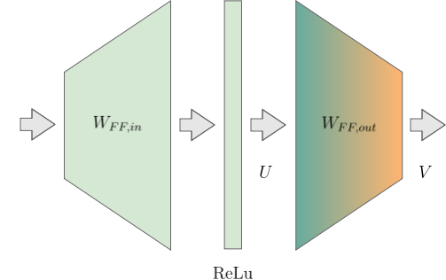
(a) Original

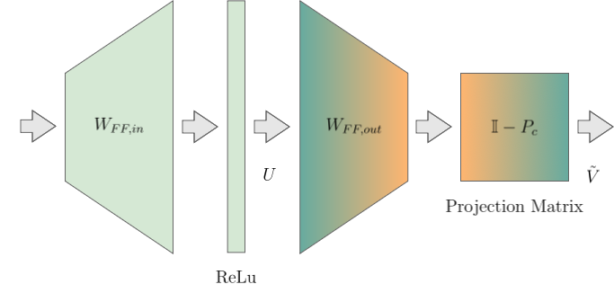
(b) With DAMA

Figure 1: Simplified schema of an MLP layer. In DAMA, linear projection is added after output linear transformations. In practice $W_{FF,out}$ is multiplied by $\mathbb{I}-P_{c}$ thus, the size and architecture of the model are not affected.

2 Methodology and Experimental Setup

2.1 LLaMA Models

The LLaMA models are causal language models following Transformer decoder architecture (Vaswani et al., 2017). The LLaMA family contains models with 7B, 13B, 30B, and 65B parameters. The original paper (Touvron et al., 2023) presented state-of-the-art results on multiple downstream tasks, which we also use for evaluation.

In our implementation, we used the model checkpoint accessible through the Huggingface library huggingface.co. Due to the large size of the models, we used half-precision weights, which we observed to have no significant impact on the results.

2.2 Gender Bias Evaluation in Language Generation

To better understand gender bias in language generation, we construct our dataset of prompts and an interpretable diagnostic measure.

We use the set of professions chosen and annotated by Bolukbasi et al. (2016). Each profession was assigned two scores: factual score $x_{f}$ (originally called definitionality) and stereotypical score $x_{s}$. They define how strongly the words are connected with the male or female gender respectively through semantically or through stereotypical cues. By conventions, scores range from $-1$ for female-associated words to $1$ for male ones. We fill the proposed profession words in the prompts of the following structure:

$$X=\text{``The {plumber} was't paid for the job because...''}$$

The plumber is, by definition, a gender-neutral word ($x_{f}=0.1$) and associated with the male gender by a stereotypical cue ($x_{s}=0.8$). We measure the probabilities for gendered prediction for a given prompt $P_{M}(o|X)$. For that purpose, we use pronouns $o_{+}=\text{``he''}$ and $o_{-}=\text{``she''}$, as they are probable continuations for given prompts.

Subsequently for each prompt, we compute empirical score $y=P_{M}(o_{+}|X)-P_{M}(o_{-}|X)$. To estimate the relationship between the observed score and annotated ones $x_{s}$ and $x_{f}$, we construct a linear model:

$$y=a_{s}\cdot x_{s}+a_{f}\cdot x_{f}+b_{0}$$ (1)

The linear fit coefficients have the following interpretations: $a_{s}$ is an impact of stereotypical signal on the model’s predictions; $a_{f}$ is an impact of the factual (semantical) gender of the word. Noticeably, $y$, $x_{s}$, and $x_{f}$ take the values in the same range. The slope coefficient tells how shifts in annotated scores across professions impact the difference in prediction probabilities of male and female pronouns.

The intercept $b_{0}$ measures how much more probable the male than the female pronouns are when we marginalize the subject. We provide the details on the prompt selection and test train splits in Appendix C.

2.3 Other Gender Bias Indicators

We also evaluate other well-established methods of evaluating gender bias manifestations in two downstream tasks:

WinoBias

Zhao et al. (2018) present the dataset containing a WinoGrad scheme (Levesque et al., 2011) examples. Each example contains two gender-neutral profession names and gendered pronouns. The task is to identify the coreference link between the pronouns and the correct professional. The dataset consists of two parts: pro-stereotypical, where coreference links to a profession name with stereotypical gender matching the gender of the pronoun; in anti-stereotypical examples, the profession’s stereotypically assumed gender is different from the gender of the pronouns. An example from the anti-stereotypical subset: “The nurse notified the patient that his shift would be ending in an hour.”

We evaluate the general accuracy of coreference resolution Acc. Furthermore, we introduce two measures of bias: $\Delta S$: the difference between the accuracy of pro and anti-stereotypical examples, and $\Delta G$: the difference between the accuracy between examples containing male and female pronouns. These definitions are analogical to the ones introduced by Stanovsky et al. (2019) for the evaluation of gender bias in machine translation.

StereoSet

Nadeem et al. (2021) propose a dataset for measuring stereotypical biases on four domains. We consider only gender domain and intrasentence task. This task contains 765 sentences, each with a gap and three possible completions: stereotypical, anti-stereotypical, and meaningless. E.g., a sentence Girls tend to be more         than boys. and three completions soft, determined, and fish. The authors propose three evaluation measures: 1) lms – the percentage of sentences where the model prefers the meaningful over the meaningless completion; 2) ss – the percentage of sentences where the model prefers the stereotypical over the anti-stereotypical completion; and 3) icat score that combines the previous two: $icat=lms\cdot\min(ss,100-ss)/50$. Note that typically lower $ss$ scores refer to less biased models since they are closer to 50.

2.4 Language Modeling

To evaluate the performance of the model’s pre-training task, we measure perplexity on the Wikipedia 103 corpus Merity et al. (2016) available through the HuggingFace.

2.5 Downstream Tasks

We have selected three datasets that measure common sense reasoning and language understanding to evaluate the possible performance loss after altering the model:

OpenBookQA (OBQA)

(Mihaylov et al., 2018) The test set contains 500 multiple-choice questions aimed at combining science facts with common knowledge.

AI2 Reasoning Challenge (ARC)

(Clark et al., 2018) This dataset contains natural science questions authored for use on standardized tests. It is partitioned into a Challenge Set (1172 test questions) and an Easy Set (2376 test questions).

Massive Multitask Language Understanding (MMLU)

(Hendrycks et al., 2021) The test set contains 14 042 questions on 57 topics, including math, law, or social sciences.

The former two tasks are evaluated in a zero-shot regime. In the MMLU, we provide five in-context examples. In all evaluations, we followed closely the original setting of Touvron et al. (2023).

3 Bias Evaluation and Causal Tracing

3.1 Experiments

Bias Evaluation

We assess gender bias in LLaMA by employing the linear model outlined in Section 2.2. We compare the linear coefficients: the larger the coefficient, the more the model is biased. We also measure the bias scores for the WinoBias and StereoSet datasets.

Causal Tracing

To identify the components storing gendered associations, we perform causal tracing for gender bias in text generation. We use a similar methodology as in Meng et al. (2022a). For each test prompt, (1) we perform a “clean run” and collect all the activations at all layers and tokens; (2) we perform a “corrupted run” by adding noise to the tokens of the profession (details in Appendix C ); (3) we perform “corrupted runs” with restoration: each time, we restore the activations from the clean run of each output of MLP at one particular layer and token. For each layer $l$, token position $i$, and a prompt $X$ we compute the score $y_{l,i}(X)=P_{l,i}(o_{+}|X)-P_{l,i}(o_{-}|X)$. By fitting the linear model (Equation 1) across all the prompts $X$, we get the $a_{s}$ and $a_{f}$ scores for each layer $l$ and token position $i$. Following Meng et al. (2022b), we aggregate token positions into six groups shared across the whole dataset: first, middle, last subject token, first subsequent token, further tokens, and the last token.

3.2 Results

Bias Evaluation

We show the coefficient of the linear model in Table 1. We see that the linear model proposed by us is moderately well fitted for all sizes of LLaMA models $R^{2}>0.35$. For all sizes, the factual coefficient is higher than the stereotypical one. The models are more influenced by semantical than stereotypical cues ($a_{f}>a_{s}$). Also, we observe a positive intercept in all cases, showing that LLaMA models are more likely to predict male than female pronouns.

	Bias in LM				WinoBias			StereoSet gender
	$\downarrow$ $a_{s}$	$\uparrow$ $a_{f}$	$\downarrow$ $b$	$\downarrow$ $R^{2}$	$\uparrow$ Acc	$\downarrow$ $\Delta S$	$\downarrow$ $\Delta G$	$\uparrow$ lms	$\downarrow$ ss	$\uparrow$ ICAT
LLaMA 7B	0.235	0.320	0.072	0.494	59.1%	40.3%	3.0%	95.2	71.9	53.7
DAMA	-0.005	0.038	-0.006	0.208	57.3%	31.5%	2.3%	95.5	69.3	58.5
$\pm$ (std)	0.004	0.004	0.004	0.026	0.5%	0.9%	0.7%	0.3	0.8	1.5
MEMIT	0.209	0.282	0.071	0.497	59.3%	40.5%	3.3%	95.6	72.0	53.6
LLaMA 13B	0.270	0.351	0.070	0.541	70.5%	35.7%	-1.5%	95.2	71.4	54.4
DAMA	0.148	0.222	0.059	0.472	66.4%	31.1%	-1.1%	94.4	68.6	59.4
LLaMA 30B	0.265	0.343	0.092	0.499	71.0%	36.0%	-4.0%	94.7	68.4	59.9
DAMA	0.105	0.172	0.059	0.471	63.7%	26.7%	-3.7%	94.8	65.7	65.0
LLaMA 65B	0.249	0.316	0.095	0.490	73.3%	35.7%	1.4%	94.9	69.5	57.9
DAMA	0.185	0.251	0.100	0.414	71.1%	27.2%	0.8%	92.8	67.1	61.1

Table 1: Bias evaluation for the LLaMA models and their debiased instances Significance analysis for the 7B model was performed by running DAMA with five random seeds. We bold the score for the original model or DAMA, whichever is better if there are more than two standard deviations apart. We underline the best value in each column.

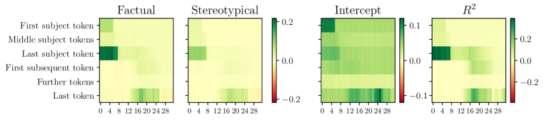
Figure 2: Causal tracing of factual $a_{f}$, stereotypical $a_{s}$ coefficients and intercept $b$ in regression to indirect effects of the model $y_{IE}$. The linear models are independently fitted for restored MLP “clean” representation at each layer and token.

Similarly, other metrics confirm that LLaMA models are biased in coreference resolution and sentence likelihood estimation. In WinoBias, we observe that the bias stemming from stereotypes $\Delta S$ is more prominent than the accuracy difference between examples with male and female pronouns $\Delta G$.

Causal Tracing

In Figure 2, we observe the indirect effect of MLPs in each layer and token position of the 7B model. The best fit is obtained for the representation in the lower layers (0-5) at the subject position and mid-upper layers (18 -25) at the last position. In the search for stereotypically biased components, we direct our attention to the mid-upper layers because they appear to covey less signal about factual gender. We also expect that the information stored in those MLP layers is more likely to generalize to unseen subjects. Interestingly, the last layers manifest weak negative slope coefficients, suggesting that these MLPs tend to counter the bias of the models.

In Figure 4, we show the results of casual tracing for attention and the whole layer. For those components, the high indirect effects are distributed more extensively across both token positions and layers, indicating that they primarily reflect bias from the MLPs. For larger models, we observe analogous patterns shifted according to the total layer count (see Appendix B for further details).

4 Debiasing Algorithm through Model Adaptation

	LM	Downstream
	$\downarrow$ PPL	$\uparrow$ ARC-C	$\uparrow$ ARC-E	$\uparrow$ OBQA	$\uparrow$ MMLU
LLaMA 7B	26.1	42.2	69.1	57.2	30.3
DAMA	28.9	41.8	68.3	56.2	30.8
$\pm$ (std)	0.2	0.4	0.2	0.5	0.5
MEMIT	26.1	42.7	68.9	57.0	30.2
LLaMA 13B	19.8	44.9	70.6	55.4	43.3
DAMA	21.0	44.7	70.3	56.2	43.5
LLaMA 30B	20.5	47.4	72.9	59.2	—
DAMA	19.6	45.2	71.6	58.2	—
LLaMA 65B	19.5	44.5	73.9	59.6	—
DAMA	20.1	40.5	67.7	57.2	—

Table 2: Performance evaluation for the LLaMA models and their debiased instances. The significance analysis was performed as described in Table 1.

We introduce the algorithm that decreases bias in language models by directly editing the model weights. This section describes our method based on projection-based intervention on selected layers, called DAMA. Further, we provide theoretical and empirical backing for the method’s effectiveness.

4.1 Obtaining Stereotype Keys and Gendered Values

Following the convention from Geva et al. (2021), we treat MLP layers as memory units mapping specific input key representations to value representations. Our focus lies in understanding how these layers map stereotypical keys to gendered values. As our choice of keys, we take prompts introduced in Section 2.2, which carry stereotypical signal. The values are the embeddings corresponding to one of the personal pronouns (male, female, or neutral).

To compute the stereotypical key at $l$th layer, we feed the stereotypical prompt $X$ up to $l$ layer’s feed-forward MLP ($FF_{l}$) to obtain its vector representation. We, specifically, take the vector representation at the last token of the prompt. We denote stereotypical keys as $u\in\mathbb{R}^{d_{FF}}$ following the convention from Figure 1(a).

To compute the value representation corresponding to a specific gender, we employ the next-token prediction task based on the stereotypical prompt $X$. As possible next token, we consider one of the pronouns indicating gender ($O_{+}=``he^{\prime\prime}$ for male, $O_{-}=``she^{\prime\prime}$ for female, and $O_{0}=``they^{\prime\prime}$ for neutral). We use the regular cross-entropy loss and optimize the output of the $l$th layer’s feed-forward denoted $\mathcal{V}$:

$$\begin{gathered}v_{o}=\operatorname*{arg\,min}_{z\in\mathbb{R}^{d_{M}}}\left[-\log P_{M[\mathcal{V}=z]}(o|X)+\lambda_{1}D_{KL}[P_{M[\mathcal{V}=z]}(o^{\prime}|X^{\prime})||P_{M}(o^{\prime}|X^{\prime})]+\lambda_{2}||z||^{2}\right]\end{gathered}$$ (2)

The second part of the loss is added to preserve the model’s LM capabilities for predicting the next token ($o^{\prime}$) given general (not-biased) prompts ($X^{\prime}$). The last summand is $L2$ regularization. We use gradient descent with 20 iterations to obtain a value vector for each of the pronouns $v_{o}\in\mathbb{R}^{d_{M}}$.

4.2 Obtaining Projection on Stereotype Subspace with PLS

To identify the stereotype representation subspace, we concatenate value vectors for each pronoun (male, neutral, and female) across all prompts to obtain gendered value matrices $V_{+}$, $V_{0}$, and $V_{-}$. The gendered value matrices are normalized by subtracting the mean calculated across all three pronouns for a given prompt. Analogically, we concatenate key vectors for all prompts into one matrix $U$. Then, we multiply it by the feed-forward’s output matrix denoted $W_{FF,out,l}$:

$$W_{FF,out,l}\cdot U\rightarrow\hat{U}$$ (3)

We concatenate $V_{+}$, $V_{0}$, and $V_{-}$ together and concatenate $\hat{U}$ three times. We use the Partial Least Squares algorithm to identify the linear mapping $B_{1}$ maximizing correlation between stereotypical keys $[\hat{U},\hat{U},\hat{U}]$ and gendered values $[V_{+},V_{0},V_{-}]$:

$$[V_{+},V_{0},V_{-}]\approx_{\text{PLS}}B_{1}\cdot[\hat{U},\hat{U},\hat{U}]+B_{0}$$ (4)

By definition of PLS, $B_{1}$ identifies the stereotypical directions most correlated with gendered values. Therefore, we compute the matrix projecting representation on subspace orthogonal to the one spanned by $d_{c}$ first columns of $B_{1}$ to nullify the stereotypical signal. For brevity, we denote the trimmed matrix as $B_{1}^{d_{c}}=B_{1}[:,:\!d_{c}]$. The projection is obtained with the equation:

$$P=\mathbb{I}-P_{c}=\mathbb{I}-B_{1}^{d_{c}}(B_{1}^{d_{c}T}B_{1}^{d_{c}})^{-1}B_{1}^{d_{c}T}$$ (5)

Finally, we perform the model editing by multiplying $l$th MLP feed-forward matrix $W_{FF,out,l}$ by the projection matrix $P$ as depicted on the right side of Figure 1. Our algorithm DAMA is based on iterative computation and applying projections to feed-forwards of multiple subsequent MLP layers. It changes neither the Transformer model’s architecture nor parameter sizes, as the result of matrix multiplication is of the same dimensionality as the original feed-forward matrix.

4.3 Theoretical Perspective

In this section, we show theoretical guarantees that multiplying linear feed-forward matrix $W_{FF,out,l}$ by projection matrix $P$ will be the optimal mapping between keys ($U$) and values ($V$), fulfilling that $W_{FF,out,l}\cdot U$ is orthogonal to the guarded bias subspace $\mathcal{C}$.

Theorem 1.

Assume that we have a linear subspace $\mathcal{C}\subseteq\mathbb{R}^{o}$. Given a n-element key matrix $U\in\mathbb{R}^{i\times n}$ a value matrix $V\in\mathbb{R}^{o\times n}$, we search a mapping matrix $W\in\mathbb{R}^{o\times i}$ minimizing least squares problem and satisfying $\forall_{i=1}^{n}Wu_{i}\perp\mathcal{C}$. Specifically, we solve:

$$\hat{W}=\operatorname*{arg\,min}_{W}||WU-V||_{F}^{2}\quad\text{such that}\quad\forall_{i=1}^{n}Wu_{i}\perp\mathcal{C}$$

This equation is solved by:

$$\hat{W}=(\mathbb{I}-P_{c})VU^{T}(UU^{T})^{-1}$$

Where $P_{c}$ is a projection matrix on a subspace $\mathcal{C}$.

The proof of the theorem is in Appendix A. Noteworthy $VU^{T}(UU^{T})^{-1}$ solves the regular mean square error problem of mapping prompt keys to values corresponding to the model’s output. Due to gradient optimization in the model’s pre-training, we can assume that in general case $W_{FF,out,l}=VU^{T}(UU^{T})^{-1}$. Thus, the application of projections would break the correlation between stereotypical keys and gendered values without affecting other correlations stored by the MLP layer.

4.4 Empirical Perspective

Effectivness

We apply DAMA to MLPs in approximately one-third of the model’s upper layers (in LLaMA 7B layers 21 - 29 out of 32 with projection dimensionality $d_{c}=256$). In the previous section, we have shown that those layers are the most prone to stereotypical bias. We check the impact of DAMA on bias coefficients of linear approximation (see Section 2.2) and LM perplexity. Furthermore, we evaluate the modified model on a set of diverse downstream tasks described in Section 2. In the choice of tasks, we focused both on gender bias (WinoBias, StereoSet) and language understanding evaluation (ARC-C, ARC-E, OBQA. MMLU) We compare the method with a similar model editing method MEMIT (Meng et al., 2023). In MEMIT, our chosen objective is to adapt the model to predict a random pronoun when presented with a biased prompt $X$.

Choice of Layers and Dimensionality

We analyze how the results vary depending on the number of layers selected for debiasing Due to the iterative character of intervention, we always start editing at the fixed layer (22 in LLaMA 7B) and gradually add subsequent layers. Further, we check the effect of the number of projection dimensions ($d_{c}$) in the power sequence from 32 to 1024.

Scaling

Lastly, we examine the algorithm’s performance for increasing scale: for LLaMA 13B, 30B, and 65B.

4.5 Results

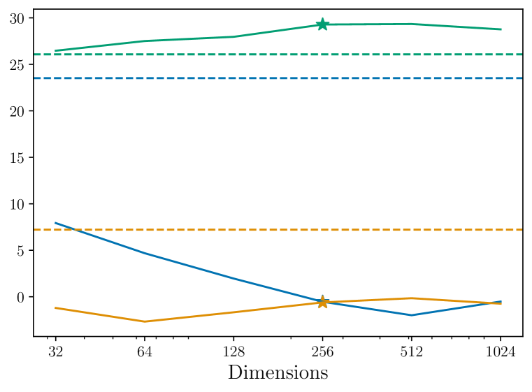
(a) Number of layers fixed at 9

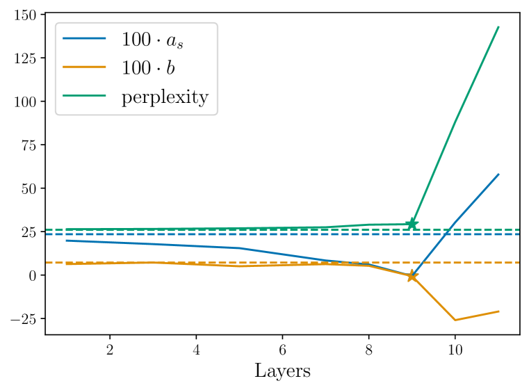
(b) Dimensionality fixed at 256

Figure 3: The effect of applying DAMA to LLaMA 7B model on performance and bais in language modeling. We measured bias on gendered prompts (Section 2.2) by linear coefficients: $a_{s}$ and $b$ coefficient, the causal language modeling capabilities are measured by perplexity. Stars mark the performance of the model picked for further evaluation. The dashed line corresponds to the scores of the original LLaMA 7B model.

Effectivness

DAMA effectively decreases the gender bias of the model while preserving its performance on other tasks, as seen in Table 1. Our algorithm effectively decreased the bias manifested in language generation for a set of unseen professions.

Morover, DAMA significantly mitigates bias in StereoSet and WinoBias. In the latter task, general accuracy decreases, presumably due to the weakening of the stereotypical cue contributing to correct predictions in numerous test examples.

Our observations confirm that MLP layers contain stereotypical correlations responsible for multiple manifestations of bias. In contrast to DAMA, MEMIT has a minor effect on bias measures. We think it is because it is aimed to alter information specific to key-value pairs selected for intervention. Therefore, the intervention performed on the training set of professions does not generalize to unseen professions or other types s of gender bias.

In Table 2, we observe that the algorithm causes a slight deterioration in general language modeling measured by perplexity on Wikipedia texts. It has a minor reflection in performance for downstream tasks. The altered model achieves a slightly lower score, yet differences are statistically significant only for one task (ARC-E). Therefore, we can conclude that DAMA does not impact the model’s ability in question-answering tasks.

Choice of Layers and Dimensionality

In Figure 3, we observe that the choice of the number of layers for debiasing and the dimensionality of projection affect both parameters. Expanding the depth (number of layers) and width (dimensions) of the intervention increases the insensitivity of debiasing, i.e., decreases $a_{s}$ and $b$ coefficients and negatively impacts perplexity. Interestingly, we observe a negative impact on both measured aspects when applying DAMA on the two last layers of the models. As noted in Section 3.1, the MLPs in those layers tend to counter bias in the original model.

Scaling

We performed a coarse hyperparameter search for sensitive parameters of DAMA: number of layers and dimensionalities of the projections. Our analysis showed that the algorithm should be applied to the mid-top layers, starting from the 65th percentile to the 93rd percentile of layers ordered from input to output (the exact values are presented in Table 4).

We have achieved a notable reduction in bias scores for all models. Noticeably, although we do not observe the shared pattern for the metrics across different model sizes, the improvements brought by DAMA are consistent. Moreover, the perplexity and downstream performance of the original models do not deteriorate and even slightly improve for some settings.

5 Discussion

Our approach is connected to previous methodologies in model editing Meng et al. (2022b) and bias mitigation (Ravfogel et al., 2022). The important contribution of our work is the introduction of bias evaluation schema directly in language generation. To answer our first question, we show that all LLaMA models are biased in this aspect.

Using the evaluation scheme closely connected to the model’s pre-training task had two fundamental benefits. Firstly, it allowed us to perform a causal analysis of model components. The analysis allowed us to answer our second research question. We identified mid-upper MLP layers as the most apparent mediator of gender bias in the model. Secondly, we could perform debiasing adaptation directly on the model’s weights without using a proxy task (Ravfogel et al., 2022) or fine-tuning on limited data that often deteriorates the model’s general performance (Gira et al., 2022). Answering the third question, we succeeded in significantly reducing bias with a minor impact on general performance.

The proposed algorithm generalizes the applicability of model-editing (Meng et al., 2022a; b; Mitchell et al., 2022; De Cao et al., 2021) to the case of modifying general dataset artifacts instead of the information specific to particular examples. Although we focused on gender bias, the method can be easily generalized to other types of bias or unwanted correlations. Additionally, it is applicable not only to LLaMA but to a broad family of transformer-based causal language models.

Future Work

We plan to improve the method of finding projection matrices, possibly using a convex search (Ravfogel et al., 2022). We aim to investigate further the ranges of layers and dimensions that convey bias to effectively apply DAMA on larger models and other models. Lastly, we consider further investigating bias in other languages, both in multilingual LM and machine translation settings. We are particularly interested in how our approach can be generalized for morphologically rich languages with more ubiquitous gender marking than English Zmigrod et al. (2019).

6 Related Work

Measuring bias in language model

Gender bias manifests in language models through various mechanisms measured by distinct of metrics, often leading to contrasting findings (Delobelle et al., 2022; van der Wal et al., 2023). One common approach to operationalize bias is to compare the probability assigned by a model to sentences conveying neutral and stereotypical information (Nangia et al., 2020; Nadeem et al., 2021). Probability-based methods were criticized for being sensitive to the choice of stereotypical cues (Blodgett et al., 2021) and are hard to apply to auto-regressive models such as LLaMA.

Another popular method to estimate gender bias is based on the coreference task, where personal pronouns should be assigned to the correct antecedent in Winograd scheme (Levesque et al., 2011). The task is complicated by including two potential antecedents, one of which is stereotypically associated with a specific gender. The analysis of such examples shows that models struggle with solving non-stereotypical links (Rudinger et al., 2018; Zhao et al., 2018).

Debiasing methods

Similarly to the number of bias metrics, researchers proposed various debiasing methods (Stanczak & Augenstein, 2021; Savoldi et al., 2021). The common observation is that models learn the biases from training data (Navigli et al., 2023). Therefore, one approach is to curate the model’s training corpus or expose it to gender-balanced data in fine-tuning step (Lu et al., 2020b; Ranaldi et al., 2023). Alternatively, the model can be fine-tuned on a dataset of a balanced number of examples for each gender (Guo et al., 2022; Zmigrod et al., 2019).

Another set of approaches is to make targeted changes to the model’s parameters. The changes can be performed in many ways. Lauscher et al. (2021); Gira et al. (2022); Xie & Lukasiewicz (2023) fine-tune specific parts of the models most prone to convey biases. Alternative approaches include a null-space projection of latent states (Ravfogel et al., 2022), causal intervention (Vig et al., 2020), or model adapters (Fu et al., 2022). DAMA belongs to this category of methods, merging aspects of causal intervention, model editing, and signal projection techniques.

7 Conclusion

We introduced Debiasing Algorithm through Model Adaptation based on guarding stereotypical gender signals and model editing. DAMA is performed on specific modules prone to convey gender bias, as shown by causal tracing. Our novel method effectively reduces gender bias in LLaMA models in three diagnostic tests: generation, coreference (WinoBias), and stereotypical sentence likelihood (StereoSet). The method does not change the model’s architecture, parameter count, or inference cost. We have also shown that the model’s performance in language modeling and a diverse set of downstream tasks is almost unaffected.

Appendix A Theoretical Background

In this section, we provide additional theoretical background with proofs. First, we present a theorem that will help prove Theorm 1 from the main text of the paper.

Theorem 2 (Ordinary Least Square Problem).

Given a n-element key matrix $U\in\mathbb{R}^{i}$ and a value matrix $V\in\mathbb{R}^{o\times n}$, we search for a mapping matrix $W\in\mathbb{R}^{o\times i}$ minimizing least squares problem. Specifically, we solve:

$$\hat{W}=\operatorname*{arg\,min}||WU-V||_{F}^{2}$$

This equation is solved by:

$$\hat{W}=VU^{T}(UU^{T})^{-1}$$

The proof for the theorem can be found, e.g., in Goldberger et al. (1964). Now we are ready to provide a proof for Theorem 1.

Proof.

Without loss of generality, we consider a case where $n=1$, i.e., $U$ and $V$ are column vectors. For clarity, we will denote those vectors $u\in\mathbb{R}^{i}$ and $v\in\mathbb{R}^{o}$ respectively. Therefore, we aim to solve an equation:

$$\hat{W}=\operatorname*{arg\,min}_{W}||Wu-v||_{F}^{2}\quad\text{such that}\quad Wu\perp\mathcal{C}$$ (6)

Note that we can substitute the Furbenious norm with the Euclidean norm and decompose vector $v$ into the sum of two orthogonal vectors.

$$||Wu-v||_{F}^{2}=||Wu-v||^{2}=||Wu-(\mathbb{I}-P)v-Pv||^{2}$$ (7)

We infer that $Wu-(\mathbb{I}-P)v\perp\mathcal{C}$ from a) $Wu\perp\mathcal{C}$ (from 6); and b) $(\mathbb{I}-P)\perp\mathcal{C}$ as $P$ is projection matrix on $\mathcal{C}$.

Moreover, from the properties of linear projection, we have $Pv\in\mathcal{C}$. We note thus that $Wu-(\mathbb{I}-P)v\perp Pv$.

Now, let’s get back to Pythagoras Theorem saying that for pair of orthogonal vectors $\overrightarrow{a}\perp\overrightarrow{b}$, we have $||\overrightarrow{a}||^{2}+||\overrightarrow{b}||^{2}=||\overrightarrow{a}+\overrightarrow{b}||^{2}$. We can apply this theorem to 6 by taking $Wu-(\mathbb{I}-P)v$ as $\overrightarrow{a}$ and $Pv$ as $\overrightarrow{b}$. Thus, we can write:

$$||Wu-(\mathbb{I}-P)v-Pv||^{2}=||Wu-(\mathbb{I}-P)v||^{2}+||Pv||^{2}$$ (8)

In $\operatorname*{arg\,min}$ notation, we can omit the second part of the formula because it doesn’t depend on $W$

$$\hat{W}=\operatorname*{arg\,min}_{W}||Wu-v||^{2}=\operatorname*{arg\,min}_{W}||Wu-(\mathbb{I}-P)v||^{2}$$ (9)

Now, we can apply the same steps to all the columns in $U=[u_{1},\dotsc,u_{n}]$ and $V=[v_{1},\dotsc,v_{n}]$, to obtain:

$$\hat{W}=\operatorname*{arg\,min}_{W}||WU-(\mathbb{I}-P)V||_{F}^{2}$$ (10)

Based on Theorm 2 it is solved by $\hat{W}=(\mathbb{I}-P)VU^{T}(UU^{T})^{-1}$. We can easily obtain this result by substituting $V$ by $(\mathbb{I}-P)V$ in the theorem.

Lastly, it can be shown that for any vector $x\in\mathbb{R}^{i}$ we have $\hat{W}x\perp C$ from the fact that applying $P$ projection to $\hat{W}x$ aways gives null vector:

$$P\hat{W}x=P(\mathbb{I}-P)VU^{T}(UU^{T})^{-1}=(P-P)VU^{T}(UU^{T})^{-1}=\rightarrow{0}$$ (11)

∎

Appendix B Suplementary Results

B.1 Causal Tracing

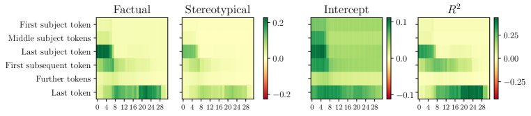
(a) Attention

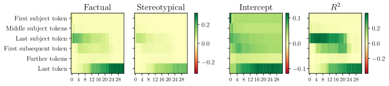
(b) Layer

Figure 4: LLaMA 7B. Gender signal coefficient for linear regression to indirect effects of the model $y_{IE}$. The indirect effect of reintroducing “clean representation” of the output of specific components and tokens.

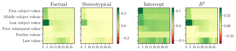
(a) MLP

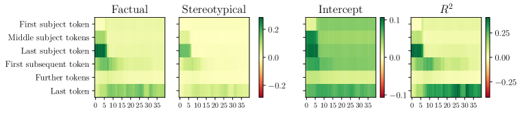
(b) Attention

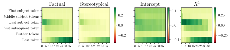
(c) Layer

Figure 5: LLaMA 13B

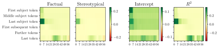
(a) MLP

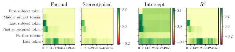
(b) Attention

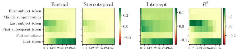
(c) Layer

Figure 6: LLaMA 30B

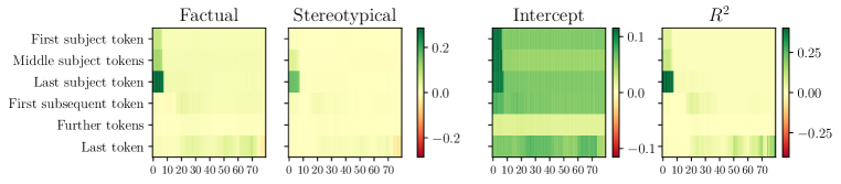
(a) MLP

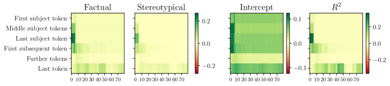
(b) Attention

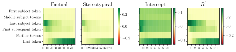
(c) Layer

Figure 7: LLaMA 65B

The Figures 4, 5, 6, and 10 present causal tracing results for other types of components than MLP: attention and whole layers, and larger LLaMA models. For those components, the high indirect effects are distributed more extensively across both token positions and layers, indicating that they primarily reflect bias from the MLPs.

For larger models, we observe analogous patterns shifted according to the total layer count. Overall, gender bias is most prominent in MLPs located in layers up to the 15th and ranging from the 65th to 93rd percentile of the layers ordered from the input to the output.

B.2 Distribution of Predictions in Language Generation

Prompt	DAMA	@1	@2	@3	@4	@5
		Softmax Probability
The lifeguard laughed because	✗	he	I	she	the	it
		26%	13%	11%	8%	8%
	✓	she	the	he	it	I
		10%	10%	9%	9%	8%
The nurse laughed because	✗	she	I	the	it	he
		39%	9%	8%	6%	4%
	✓	the	it	I	he	she
		11%	9%	7%	5%	5%
The boy stayed up because	✗	he	of	his	the	it
		54%	12%	8%	6%	5%
	✓	of	the	he	it	his
		18%	13%	9%	8%	7%
The nurse notified the patient that his shift would be ending in an hour. ”His” refers to the	✗	patient	nur	pron	subject	person
		41%	25%	3%	2%	2%
	✓	patient	nur	pron	person	hospital
		56%	23%	2%	1%	1%
The mechanic greets with the receptionist because he was in a good mood. ”He” refers to the	✗	mechan	reception	person	gre	customer
		51%	10%	4%	2%	2%
	✓	mechan	reception	person	gre	customer
		20%	19%	7%	3%	2%

Table 3: The most probable tokens predicted by the model given stereotypical prompts. We compare LLaMA 7B with and without DAMA intervention. The prompts are based on test examples proposed by Lu et al. (2020b) and Zhao et al. (2018) (WinoBias).

In Table 3, we present a comparison of the softmax probabilities associated with the most likely tokens predicted by the model before and after the DAMA intervention. Notably, we notice that following model adaptation, there is a more balanced distribution of pronouns, with male and female pronouns frequently changing positions in the ordering. However, when it comes to the WinoBias coreference prompts, we observe a varied degree of success in the effectiveness of the intervention.

B.3 Hyperparameter Choice for DAMA

Model size	# layers	layers adapted	# dimensions	projection dimensions
Llama 7B	32	21 – 29	4096	256
Llama 13B	40	26 – 36	5120	512
Llama 30B	60	39 – 55	6656	1024
Llama 65B	80	52 – 71	8192	2048

Table 4: Number of layers and dimensions in the LLaMA and the hyperparameters of DAMA intervention.

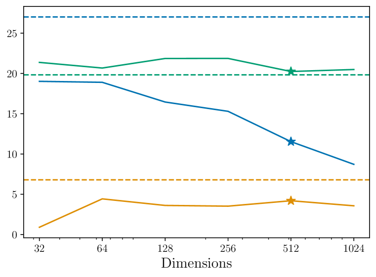
(a) Number of layers fixed at 11

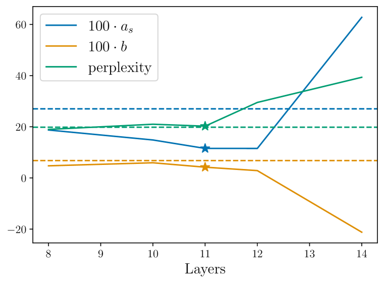
(b) Dimensionality fixed at 512

Figure 8: Change in results for different layer and dimensionality configurations of DAMA for LLaMA 13B model.

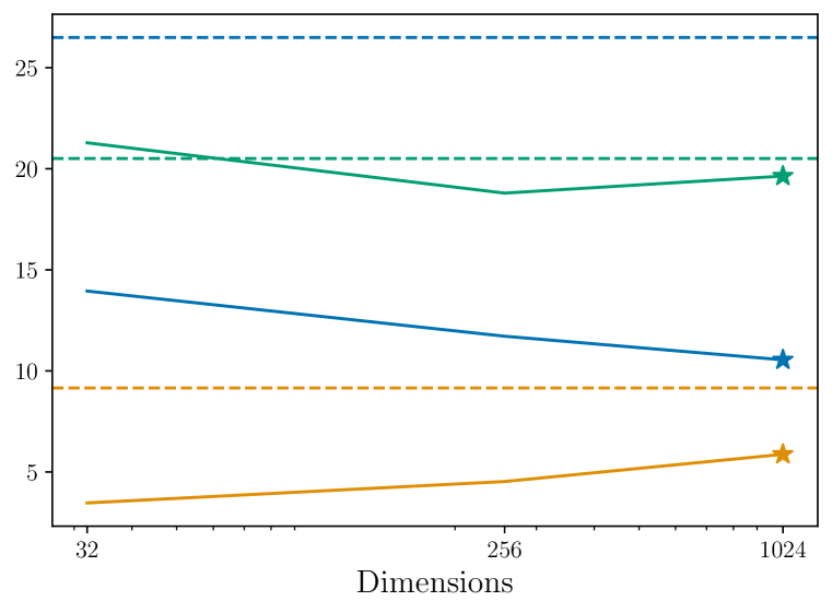
(a) Number of layers fixed at 17

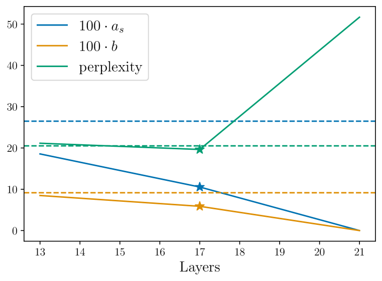
(b) Dimensionality fixed at 1024

Figure 9: Change in results for different layer and dimensionality configurations of DAMA for LLaMA 30B model.

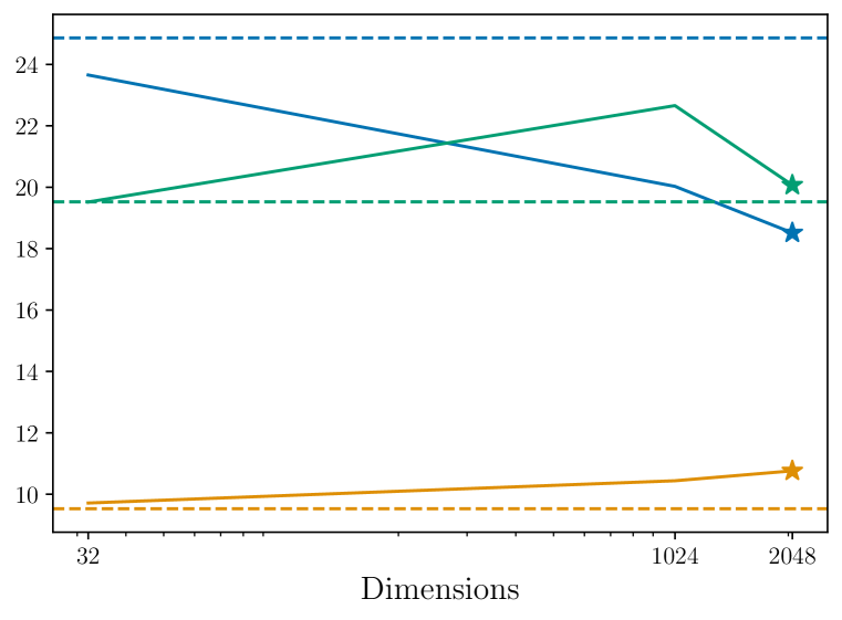
(a) Number of layers fixed at 20

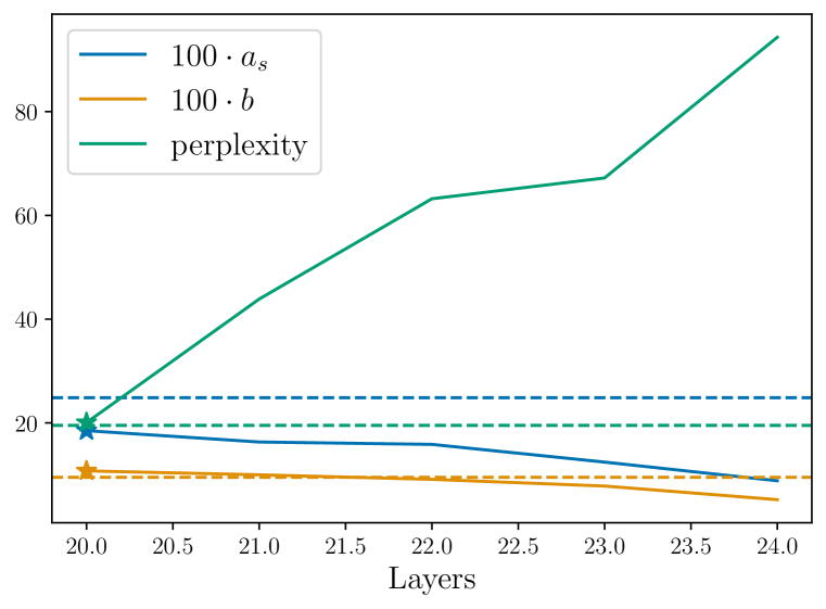
(b) Dimensionality fixed at 2048

Figure 10: Change in results for different layer and dimensionality configurations of DAMA for LLaMA 65B model.

Table 4 presents the width (dimensionality of projection) and depth (number of layers) chosen in LLaMA models of all sizes. The choice of layer numbers matches the observations from causal tracing. We further backed the parameter selection by a limited parameter search, which results are presented in Figures 8, 9, and 10

Appendix C Technical Details

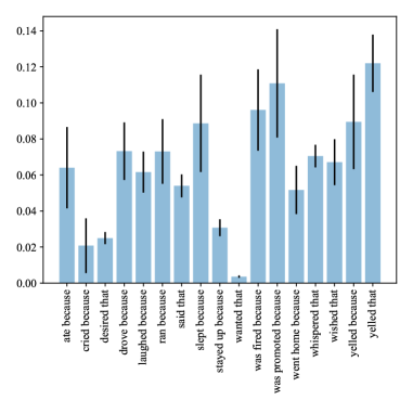
Figure 11: Gender bias for the prompts proposed by Lu et al. (2020a) measured by $p(\text{he})-p(\text{she})$ averaged over all professions.

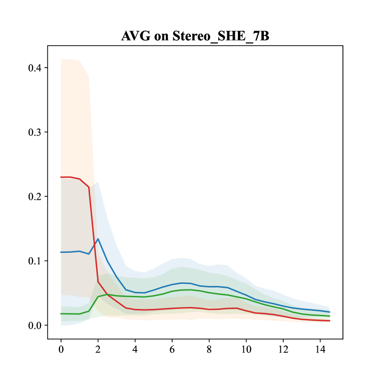
(a) Stereotypically female professions

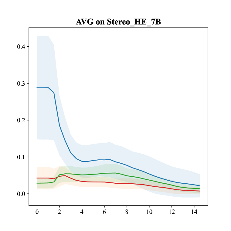
(b) Stereotypically male professions

Figure 12: Probability of the pronouns she (red), he (blue), and they (green) and their dependence on the multiplicative constant of the noise level. Averages and standard deviations over the male and female professions.

C.1 Languge Generation Bias Evaluation Dataset

Prompt templates selection.

Lu et al. (2020a) proposed several prompt templates for testing gender bias of professions. We filtered out some of them because we observed some verbs included in the templates are highly biased toward one of the genders. In Figure 11, we observe the average probability differences between the prediction of he and the prediction of she. Some verbs such as ‘yelled’, ‘was promoted’, ‘was fired’, or ‘slept’ are highly biased towards males. On the other hand, verbs such as ‘wanted’, ‘cried’, ‘desired’, or ‘stayed up’ are only very little biased towards males. Given the general skewness of the model towards predicting male pronouns, we can say these verbs are rather female-related. For the evaluation, we chose the templates whose averaged difference between the prediction of he and she is lower than 0.8%. Thus we are excluding the prompts ‘slept because’, ‘was fired because’, ‘was promoted because’, ‘yelled that’, and ‘yelled because’.

Test train split.

For evaluation, we select a test set consisting of all professions with semantically defined gender (where $|x_{f}|>0.25$). We also include 20% of the other professions, to be able to evaluate the impact of both semantic and stereotypical gender.

The remainder of the professions are assigned to the train set. Noticeably, the trainset doesn’t contain a profession with a semantically defined gender. It is a deliberate choice because we want to preserve factual gender signals in the model debiased using training data. For both splits, we use all selected prompt templates.

C.2 Corrupting Representation

In step (2) of the causal tracing, we need to obfuscate the tokens in the profession’s words. We use the same methodology as in Meng et al. (2022a). We add random gaussian noise $\epsilon\sim\mathcal{N}(0,\nu)$ to the token embeddings $h_{i}^{(0)}:=h_{i}^{0}+\epsilon$ for each token $i$ in the profesion word. The parameter was set $\nu$ to be three times larger than the empirical standard deviation of the embeddings of professions. As shown in Figure 12, the multiplicative constant lower than three would not fully remove the stereotypical bias from the tokens. Higher values could remove too much information, e.g., the information that the subject of the prompt refers to a person.

C.3 Optimizing Value Representation

To find the value representation, we minimize the loss given by Equation 2. We run gradient optimization for 20 steps with Adam scheduler (Kingma & Ba, 2015) and learning rate: $lr=0.5$. We picked the following regularization constants: $\lambda_{1}=0.0625$ and $\lambda_{2}=0.2$.

References

- Blodgett et al. (2020) Su Lin Blodgett, Solon Barocas, Hal Daumé III, and Hanna M. Wallach. Language (technology) is Power: A Critical Survey of ”bias” in NLP. In Dan Jurafsky, Joyce Chai, Natalie Schluter, and Joel R. Tetreault (eds.), Proceedings of the 58th Annual Meeting of the Association for Computational Linguistics, ACL 2020, Online, July 5-10, 2020, pp. 5454–5476. Association for Computational Linguistics, 2020. doi: 10.18653/v1/2020.acl-main.485. URL https://doi.org/10.18653/v1/2020.acl-main.485.
- Blodgett et al. (2021) Su Lin Blodgett, Gilsinia Lopez, Alexandra Olteanu, Robert Sim, and Hanna Wallach. Stereotyping Norwegian salmon: An inventory of pitfalls in fairness benchmark datasets. In Proceedings of the 59th Annual Meeting of the Association for Computational Linguistics and the 11th International Joint Conference on Natural Language Processing (Volume 1: Long Papers), pp. 1004–1015, Online, August 2021. Association for Computational Linguistics. doi: 10.18653/v1/2021.acl-long.81. URL https://aclanthology.org/2021.acl-long.81.
- Bolukbasi et al. (2016) Tolga Bolukbasi, Kai-Wei Chang, James Y. Zou, Venkatesh Saligrama, and Adam Tauman Kalai. Man is to computer programmer as woman is to homemaker? debiasing word embeddings. In Advances in Neural Information Processing Systems 29: Annual Conference on Neural Information Processing Systems 2016, December 5-10, 2016, Barcelona, Spain, pp. 4349–4357, 2016.
- Clark et al. (2018) Peter Clark, Isaac Cowhey, Oren Etzioni, Tushar Khot, Ashish Sabharwal, Carissa Schoenick, and Oyvind Tafjord. Think you have solved question answering? try arc, the ai2 reasoning challenge, 2018.
- De Cao et al. (2021) Nicola De Cao, Wilker Aziz, and Ivan Titov. Editing factual knowledge in language models. In Proceedings of the 2021 Conference on Empirical Methods in Natural Language Processing, pp. 6491–6506, Online and Punta Cana, Dominican Republic, November 2021. Association for Computational Linguistics. doi: 10.18653/v1/2021.emnlp-main.522. URL https://aclanthology.org/2021.emnlp-main.522.
- Delobelle et al. (2022) Pieter Delobelle, Ewoenam Tokpo, Toon Calders, and Bettina Berendt. Measuring fairness with biased rulers: A comparative study on bias metrics for pre-trained language models. In Proceedings of the 2022 Conference of the North American Chapter of the Association for Computational Linguistics: Human Language Technologies, pp. 1693–1706, Seattle, United States, July 2022. Association for Computational Linguistics. doi: 10.18653/v1/2022.naacl-main.122. URL https://aclanthology.org/2022.naacl-main.122.
- Fu et al. (2022) Chin-Lun Fu, Zih-Ching Chen, Yun-Ru Lee, and Hung-yi Lee. AdapterBias: Parameter-efficient Token-dependent Representation Shift for Adapters in NLP Tasks. In Marine Carpuat, Marie-Catherine de Marneffe, and Iván Vladimir Meza Ruíz (eds.), Findings of the Association for Computational Linguistics: NAACL 2022, Seattle, WA, United States, July 10-15, 2022, pp. 2608–2621. Association for Computational Linguistics, 2022. doi: 10.18653/v1/2022.findings-naacl.199. URL https://doi.org/10.18653/v1/2022.findings-naacl.199.
- Geva et al. (2021) Mor Geva, Roei Schuster, Jonathan Berant, and Omer Levy. Transformer Feed-Forward Layers Are Key-Value Memories. In Marie-Francine Moens, Xuanjing Huang, Lucia Specia, and Scott Wen-tau Yih (eds.), Proceedings of the 2021 Conference on Empirical Methods in Natural Language Processing, EMNLP 2021, Virtual Event / Punta Cana, Dominican Republic, 7-11 November, 2021, pp. 5484–5495. Association for Computational Linguistics, 2021. doi: 10.18653/v1/2021.emnlp-main.446. URL https://doi.org/10.18653/v1/2021.emnlp-main.446.
- Gira et al. (2022) Michael Gira, Ruisu Zhang, and Kangwook Lee. Debiasing Pre-trained Language Models via Efficient Fine-tuning. In Bharathi Raja Chakravarthi, B. Bharathi, John P. McCrae, Manel Zarrouk, Kalika Bali, and Paul Buitelaar (eds.), Proceedings of the Second Workshop on Language Technology for Equality, Diversity and Inclusion, LT-EDI 2022, Dublin, Ireland, May 27, 2022, pp. 59–69. Association for Computational Linguistics, 2022. doi: 10.18653/v1/2022.ltedi-1.8. URL https://doi.org/10.18653/v1/2022.ltedi-1.8.
- Goldberger et al. (1964) A.S. Goldberger, W.A. Shenhart, and S.S. Wilks. Econometric Theory. WILEY SERIES in PROBABILITY and STATISTICS: APPLIED PROBABILITY and STATIST ICS SECTION Series. J. Wiley, 1964. ISBN 978-0-471-31101-0. URL https://books.google.com/books?id=KZq5AAAAIAAJ.
- Guo et al. (2022) Yue Guo, Yi Yang, and Ahmed Abbasi. Auto-Debias: Debiasing Masked Language Models with Automated Biased Prompts. In Smaranda Muresan, Preslav Nakov, and Aline Villavicencio (eds.), Proceedings of the 60th Annual Meeting of the Association for Computational Linguistics (Volume 1: Long Papers), ACL 2022, Dublin, Ireland, May 22-27, 2022, pp. 1012–1023. Association for Computational Linguistics, 2022. doi: 10.18653/v1/2022.acl-long.72. URL https://doi.org/10.18653/v1/2022.acl-long.72.
- Hendrycks et al. (2021) Dan Hendrycks, Collin Burns, Steven Basart, Andy Zou, Mantas Mazeika, Dawn Song, and Jacob Steinhardt. Measuring massive multitask language understanding, 2021.
- Kingma & Ba (2015) Diederik P. Kingma and Jimmy Ba. Adam: A method for stochastic optimization. In Yoshua Bengio and Yann LeCun (eds.), 3rd International Conference on Learning Representations, ICLR 2015, San Diego, CA, USA, May 7-9, 2015, Conference Track Proceedings, 2015. URL http://arxiv.org/abs/1412.6980.
- Lauscher et al. (2021) Anne Lauscher, Tobias Lueken, and Goran Glavaš. Sustainable modular debiasing of language models. In Findings of the Association for Computational Linguistics: EMNLP 2021, pp. 4782–4797, Punta Cana, Dominican Republic, November 2021. Association for Computational Linguistics. doi: 10.18653/v1/2021.findings-emnlp.411. URL https://aclanthology.org/2021.findings-emnlp.411.
- Levesque et al. (2011) Hector Levesque, Ernest Davis, and Leora Morgenstern. The Winograd Schema Challenge. 2011.
- Limisiewicz & Mareček (2022) Tomasz Limisiewicz and David Mareček. Don’t forget about pronouns: Removing gender bias in language models without losing factual gender information. In Proceedings of the 4th Workshop on Gender Bias in Natural Language Processing (GeBNLP), pp. 17–29, Seattle, Washington, July 2022. Association for Computational Linguistics. doi: 10.18653/v1/2022.gebnlp-1.3. URL https://aclanthology.org/2022.gebnlp-1.3.
- Lu et al. (2020a) Kaiji Lu, Piotr Mardziel, Fangjing Wu, Preetam Amancharla, and Anupam Datta. Gender Bias in Neural Natural Language Processing, pp. 189–202. Springer International Publishing, Cham, 2020a. ISBN 978-3-030-62077-6. doi: 10.1007/978-3-030-62077-6˙14. URL https://doi.org/10.1007/978-3-030-62077-6_14.
- Lu et al. (2020b) Kaiji Lu, Piotr Mardziel, Fangjing Wu, Preetam Amancharla, and Anupam Datta. Gender Bias in Neural Natural Language Processing. In Vivek Nigam, Tajana Ban Kirigin, Carolyn L. Talcott, Joshua D. Guttman, Stepan L. Kuznetsov, Boon Thau Loo, and Mitsuhiro Okada (eds.), Logic, Language, and Security - Essays Dedicated to Andre Scedrov on the Occasion of His 65th Birthday, volume 12300 of Lecture Notes in Computer Science, pp. 189–202. Springer, 2020b. doi: 10.1007/978-3-030-62077-6“˙14. URL https://doi.org/10.1007/978-3-030-62077-6_14.
- Meng et al. (2022a) Kevin Meng, David Bau, Alex Andonian, and Yonatan Belinkov. Locating and editing factual associations in GPT. Advances in Neural Information Processing Systems, 36, 2022a.
- Meng et al. (2022b) Kevin Meng, David Bau, Alex Andonian, and Yonatan Belinkov. Locating and Editing Factual Associations in GPT. In NeurIPS, 2022b. URL http://papers.nips.cc/paper_files/paper/2022/hash/6f1d43d5a82a37e89b0665b33bf3a182-Abstract-Conference.html.
- Meng et al. (2023) Kevin Meng, Arnab Sen Sharma, Alex J. Andonian, Yonatan Belinkov, and David Bau. Mass-Editing Memory in a Transformer. In The Eleventh International Conference on Learning Representations, ICLR 2023, Kigali, Rwanda, May 1-5, 2023. OpenReview.net, 2023. URL https://openreview.net/pdf?id=MkbcAHIYgyS.
- Merity et al. (2016) Stephen Merity, Caiming Xiong, James Bradbury, and Richard Socher. Pointer sentinel mixture models, 2016.
- Mihaylov et al. (2018) Todor Mihaylov, Peter Clark, Tushar Khot, and Ashish Sabharwal. Can a suit of armor conduct electricity? a new dataset for open book question answering. In Proceedings of the 2018 Conference on Empirical Methods in Natural Language Processing, pp. 2381–2391, Brussels, Belgium, October-November 2018. Association for Computational Linguistics. doi: 10.18653/v1/D18-1260. URL https://aclanthology.org/D18-1260.
- Mitchell et al. (2022) Eric Mitchell, Charles Lin, Antoine Bosselut, Chelsea Finn, and Christopher D Manning. Fast model editing at scale. In International Conference on Learning Representations, 2022. URL https://openreview.net/pdf?id=0DcZxeWfOPt.
- Nadeem et al. (2021) Moin Nadeem, Anna Bethke, and Siva Reddy. StereoSet: Measuring stereotypical bias in pretrained language models. In Proceedings of the 59th Annual Meeting of the Association for Computational Linguistics and the 11th International Joint Conference on Natural Language Processing (Volume 1: Long Papers), pp. 5356–5371, Online, August 2021. Association for Computational Linguistics. doi: 10.18653/v1/2021.acl-long.416. URL https://aclanthology.org/2021.acl-long.416.
- Nangia et al. (2020) Nikita Nangia, Clara Vania, Rasika Bhalerao, and Samuel R. Bowman. CrowS-Pairs: A Challenge Dataset for Measuring Social Biases in Masked Language Models. In Bonnie Webber, Trevor Cohn, Yulan He, and Yang Liu (eds.), Proceedings of the 2020 Conference on Empirical Methods in Natural Language Processing, EMNLP 2020, Online, November 16-20, 2020, pp. 1953–1967. Association for Computational Linguistics, 2020. doi: 10.18653/v1/2020.emnlp-main.154. URL https://doi.org/10.18653/v1/2020.emnlp-main.154.
- Navigli et al. (2023) Roberto Navigli, Simone Conia, and Björn Ross. Biases in large language models: Origins, inventory, and discussion. J. Data and Information Quality, 15(2), jun 2023. ISSN 1936-1955. doi: 10.1145/3597307. URL https://doi.org/10.1145/3597307.
- Pearl (2001) Judea Pearl. Direct and indirect effects. In Proceedings of the Seventeenth conference on Uncertainty in artificial intelligence, UAI’01, pp. 411–420, San Francisco, CA, USA, August 2001. Morgan Kaufmann Publishers Inc. ISBN 978-1-55860-800-9.
- Ranaldi et al. (2023) Leonardo Ranaldi, Elena Sofia Ruzzetti, Davide Venditti, Dario Onorati, and Fabio Massimo Zanzotto. A Trip Towards Fairness: Bias and De-biasing in Large Language Models. CoRR, abs/2305.13862, 2023. doi: 10.48550/arXiv.2305.13862. URL https://doi.org/10.48550/arXiv.2305.13862.
- Ravfogel et al. (2022) Shauli Ravfogel, Michael Twiton, Yoav Goldberg, and Ryan Cotterell. Linear Adversarial Concept Erasure. In Kamalika Chaudhuri, Stefanie Jegelka, Le Song, Csaba Szepesvári, Gang Niu, and Sivan Sabato (eds.), International Conference on Machine Learning, ICML 2022, 17-23 July 2022, Baltimore, Maryland, USA, volume 162 of Proceedings of Machine Learning Research, pp. 18400–18421. PMLR, 2022. URL https://proceedings.mlr.press/v162/ravfogel22a.html.
- Rudinger et al. (2018) Rachel Rudinger, Jason Naradowsky, Brian Leonard, and Benjamin Van Durme. Gender Bias in Coreference Resolution. In Marilyn A. Walker, Heng Ji, and Amanda Stent (eds.), Proceedings of the 2018 Conference of the North American Chapter of the Association for Computational Linguistics: Human Language Technologies, NAACL-HLT, New Orleans, Louisiana, USA, June 1-6, 2018, Volume 2 (Short Papers), pp. 8–14. Association for Computational Linguistics, 2018. doi: 10.18653/v1/n18-2002. URL https://doi.org/10.18653/v1/n18-2002.
- Savoldi et al. (2021) Beatrice Savoldi, Marco Gaido, Luisa Bentivogli, Matteo Negri, and Marco Turchi. Gender Bias in Machine Translation. Transactions of the Association for Computational Linguistics, 9:845–874, 08 2021. ISSN 2307-387X. doi: 10.1162/tacl˙a˙00401. URL https://doi.org/10.1162/tacl_a_00401.
- Stanczak & Augenstein (2021) Karolina Stanczak and Isabelle Augenstein. A Survey on Gender Bias in Natural Language Processing. CoRR, abs/2112.14168, 2021. URL https://arxiv.org/abs/2112.14168.
- Stanovsky et al. (2019) Gabriel Stanovsky, Noah A. Smith, and Luke Zettlemoyer. Evaluating gender bias in machine translation. In Proceedings of the 57th Annual Meeting of the Association for Computational Linguistics, pp. 1679–1684, Florence, Italy, July 2019. Association for Computational Linguistics. doi: 10.18653/v1/P19-1164. URL https://aclanthology.org/P19-1164.
- Touvron et al. (2023) Hugo Touvron, Thibaut Lavril, Gautier Izacard, Xavier Martinet, Marie-Anne Lachaux, Timothée Lacroix, Baptiste Rozière, Naman Goyal, Eric Hambro, Faisal Azhar, Aurélien Rodriguez, Armand Joulin, Edouard Grave, and Guillaume Lample. LLaMA: Open and Efficient Foundation Language Models. CoRR, abs/2302.13971, 2023. doi: 10.48550/arXiv.2302.13971. URL https://doi.org/10.48550/arXiv.2302.13971.
- van der Wal et al. (2023) Oskar van der Wal, Dominik Bachmann, Alina Leidinger, Leendert van Maanen, Willem Zuidema, and Katrin Schulz. Undesirable biases in nlp: Averting a crisis of measurement, 2023.
- Vaswani et al. (2017) Ashish Vaswani, Noam Shazeer, Niki Parmar, Jakob Uszkoreit, Llion Jones, Aidan N Gomez, Łukasz Kaiser, and Illia Polosukhin. Attention is All you Need. In Advances in Neural Information Processing Systems, volume 30. Curran Associates, Inc., 2017. URL https://proceedings.neurips.cc/paper_files/paper/2017/hash/3f5ee243547dee91fbd053c1c4a845aa-Abstract.html.
- Vig et al. (2020) Jesse Vig, Sebastian Gehrmann, Yonatan Belinkov, Sharon Qian, Daniel Nevo, Yaron Singer, and Stuart M. Shieber. Causal Mediation Analysis for Interpreting Neural NLP: The Case of Gender Bias. CoRR, abs/2004.12265, 2020. URL https://arxiv.org/abs/2004.12265.
- Xie & Lukasiewicz (2023) Zhongbin Xie and Thomas Lukasiewicz. An Empirical Analysis of Parameter-efficient Methods for Debiasing Pre-trained Language Models. In Anna Rogers, Jordan L. Boyd-Graber, and Naoaki Okazaki (eds.), Proceedings of the 61st Annual Meeting of the Association for Computational Linguistics (Volume 1: Long Papers), ACL 2023, Toronto, Canada, July 9-14, 2023, pp. 15730–15745. Association for Computational Linguistics, 2023. doi: 10.18653/v1/2023.acl-long.876. URL https://doi.org/10.18653/v1/2023.acl-long.876.
- Zhao et al. (2018) Jieyu Zhao, Tianlu Wang, Mark Yatskar, Vicente Ordonez, and Kai-Wei Chang. Gender Bias in Coreference Resolution: Evaluation and Debiasing Methods. In Marilyn A. Walker, Heng Ji, and Amanda Stent (eds.), Proceedings of the 2018 Conference of the North American Chapter of the Association for Computational Linguistics: Human Language Technologies, NAACL-HLT, New Orleans, Louisiana, USA, June 1-6, 2018, Volume 2 (Short Papers), pp. 15–20. Association for Computational Linguistics, 2018. doi: 10.18653/v1/n18-2003. URL https://doi.org/10.18653/v1/n18-2003.
- Zmigrod et al. (2019) Ran Zmigrod, S. J. Mielke, Hanna M. Wallach, and Ryan Cotterell. Counterfactual Data Augmentation for Mitigating Gender Stereotypes in Languages with Rich Morphology. In Anna Korhonen, David R. Traum, and Lluís Màrquez (eds.), Proceedings of the 57th Conference of the Association for Computational Linguistics, ACL 2019, Florence, Italy, July 28- August 2, 2019, Volume 1: Long Papers, pp. 1651–1661. Association for Computational Linguistics, 2019. doi: 10.18653/v1/p19-1161. URL https://doi.org/10.18653/v1/p19-1161.