Incorporating nonparametric methods for estimating causal excursion effects in mobile health with zero-inflated count outcomes

Abstract

In the domain of mobile health, tailoring interventions for real-time delivery is of paramount importance. Micro-randomized trials have emerged as the “gold-standard” methodology for developing such interventions. Analyzing data from these trials provides insights into the efficacy of interventions and the potential moderation by specific covariates. The “causal excursion effect", a novel class of causal estimand, addresses these inquiries, backed by current semiparametric inference techniques. Yet, existing methods mainly focus on continuous or binary data, leaving count data largely unexplored. The current work is motivated by the Drink Less micro-randomized trial from the UK, which focuses on a zero-inflated proximal outcome, the number of screen views in the subsequent hour following the intervention decision point. In the current paper, we revisit the concept of causal excursion effects, specifically for zero-inflated count outcomes, and introduce novel estimation approaches that incorporate nonparametric techniques. Bidirectional asymptotics are derived for the proposed estimators. Through extensive simulation studies, we evaluate the performance of the proposed estimators. As an illustration, we also employ the proposed methods to the Drink Less trial data.

Keywords Count outcome  $\cdot$ Causal excursion effect  $\cdot$ Micro-randomized trial  $\cdot$ Mobile health  $\cdot$ Structural nested mean model

1 Introduction

Mobile health (mHealth) interventions, particularly those utilizing text messages or push notifications, have been developed to promote health-related behaviors. These interventions exhibit significant potential across a wide range of health issues, from alcohol consumption reduction (Song et al., 2019) to physical activity maintenance (Lee et al., 2019). Advancements in mobile and sensing technologies now facilitate real-time tracking of an individual’s internal state and context, offering timely and personalized support (Kumar et al., 2013; Spruijt-Metz and Nilsen, 2014). This has given rise to the concept of the just-in-time adaptive intervention (JITAI), a method that tailors treatment in response to the evolving needs and situations of the individual, bearing the goal of delivering the right treatment on the right occasion (Nahum-Shani et al., 2018). For instance, the evening, recognized as a high-risk window for individuals with a history of excessive alcohol consumption, might be ideal for targeted interventions (Day et al., 2014; Bell et al., 2020).

The micro-randomized trial (MRT) has emerged as the touchstone methodology for devising these interventions (Klasnja et al., 2015; Liao et al., 2016). Within the framework of an MRT, participants undergo sequential randomization, aligning them with one of the intervention options across hundreds or even thousands of decision points. Typically, data analysis from micro-randomized trials seeks to answer three critical scientific questions: (1) which interventions can impact the proximal outcome; (2) in which context should the intervention be delivered; and (3) does the treatment effect change with time? The “causal excursion effect", a novel class of causal estimand, provides solutions to these inquiries (Boruvka et al., 2018; Qian et al., 2021a). Notably, these effects can be perceived as a marginal generalization of the treatment “blips" in the structural nested mean model (Robins, 1989, 1994), as they are conditional on a few selected variables instead of all past observed variables.

To estimate the causal excursion effect, one might consider using standard methods such as generalized estimating equation (GEE) approaches (Liang and Zeger, 1986) or random-effects models (Laird and Ware, 1982), especially given the longitudinal nature of data from mHealth studies. Yet, these methods are not guaranteed to give consistent estimates of treatment effects when the data includes both time-varying treatments and time-varying confounders (Sullivan Pepe and Anderson, 1994; Robins and Hernan, 2008). Structural nested mean models have been proposed to address this issue by modeling the causal effects of a time-varying treatment on a time-varying outcome (Robins, 1994). Augmenting this, the G-estimation methodology offers an effective toolset for isolating treatment effects in the presence of time-varying confounding.

In the evolving landscape of MRT-related methodologies, both Boruvka et al. (2018) and Qian et al. (2021a) have innovatively expanded upon the concept, enabling the estimation of causal excursion effects through a weighted and centered least square estimator. However, these studies focus on either continuous or binary data, leaving count data largely unexplored. Our study is motivated by the Drink Less trial where the proximal outcome is the user’s engagement with the mobile app, measured by the number of screen views in the subsequent hour following the notification decision point (Bell et al., 2020). Notably, this outcome has a unique characteristic of being zero-inflated as under certain contexts or intervention conditions users may rarely open the app, thereby consistently recording zero screen views. Consequently, common distributional assumptions such as normal or binomial distribution are no longer tenable for such data.

In this paper, we revisit the concept of causal excursion effects under potentially zero-inflated count outcomes and introduce novel estimation methodologies. As highlighted by Shi and Dempsey (2023), even within MRTs, the accurate collection of randomization probabilities can be compromised due to technical errors. To this end, we propose a class of doubly robust estimating equations applicable to both MRTs and observational mHealth studies, even when treatments are not randomized. Our work yields three primary contributions:

1. We revisit causal excursion effects and the weighted and centered least square estimator, also known as the estimator of the marginal excursion effect (EMEE) from Qian et al. (2021a), focusing on zero-inflated count outcomes.

2. We advocate for nonparametric techniques to estimate nuisance functions, such as generalized additive models. In particular, we adopt a two-part model for estimating the conditional mean of the proximal outcomes to adapt to the zero-inflation nature.

3. We propose a doubly-robust estimator to estimate the causal excursion effect. The resulting estimator is consistent and asymptotically normal provided the convergence rates of nuisance function estimators are sufficiently fast, known as rate double robustness (Yu et al., 2023). Moreover, we establish bidirectional asymptotics, which require either the sample size or the number of decision points to go to infinity.

The rest of this article is organized as follows. Section 2 provides an overview of the Drink Less trial as a motivating example. The notation and causal estimand are reviewed in Section 3. Section 4 details the incorporation of nonparametric methods for estimating the causal excursion effect. Section 5 provides the data generation procedure, settings, and results of the simulation study. Next, we apply the proposed method to analyzing the Drink Less data in Section 6. We conclude with a discussion in Section 7.

2 Motivating example: Drink Less

Our motivating example is from an mHealth app named Drink Less. This app targets the general UK adults who are drinking alcohol at increasing and higher risk levels in reducing hazardous and harmful alcohol consumption (Garnett et al., 2019, 2021). However, a decline in user engagement can notably affect the app’s effectiveness.

The MRT design offers a robust experimental framework, producing quality data that can enhance the timing, content, and delivery sequence of mHealth interventions (Klasnja et al., 2015; Liao et al., 2016; Qian et al., 2022; Liu et al., 2023). Participants in MRTs are sequentially randomized to receive varying intervention options, such as receiving a push notification or not. Along with each intervention, data on proximal outcomes and covariates are also gathered, resulting in a collection of time-varying covariates, interventions, and proximal outcomes. The primary objective of MRTs is to inform the design of JITAIs embedded in behavior change apps by assessing the proximal effects of treatments and how covariates might influence those effects.

A 30-day MRT with 349 participants was conducted to improve the push notification strategy in Drink Less (Bell et al., 2020). Participants with a baseline Alcohol Use Disorders Identification Test (AUDIT) score of 8 or higher (Bohn et al., 1995; Saunders et al., 1993), who resided in the UK, were at least 18 years old, and desired to drink less, were recruited into the trial. Every day at 8 p.m., during the trial, participants were randomly given one of three intervention options: no notification, the standard notification, or a message randomly selected from a new message bank. For more details about the messages, see Bell et al. (2020). Each option was assigned according to a static randomization probability of 40%, 30%, and 30%, respectively. The depth of engagement with the app was measured by the total number of screen views between 8 p.m. and 9 p.m. Along with the interventions, data on age, AUDIT score, gender, and other covariates were also recorded. The main goal is to explore the effects of push notifications on user engagement, whether or not these effects differ according to the user’s context, and how these effects change over time.

We first examine the distribution of the proximal outcome from the Drink Less trial. Figure 1 displays the histogram and Q-Q plot of the proximal outcome, which is the number of screen views between 8 p.m. and 9 p.m. following no notification, a new notification, or the standard notification. The results suggest that the proximal outcome is not normally distributed and is highly zero-inflated.

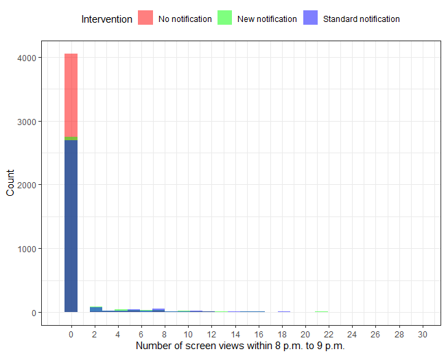
(a) Histogram

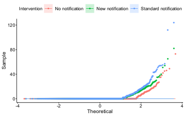
(b) Q-Q plot

Figure 1: Graphical inspection of the distribution and normality check of the number of screen views from 8 p.m. to 9 p.m. after each type of notification.

3 Causal Excursion Effect: A Review

3.1 Notations

Consider a setting with longitudinal data spanning $T$ decision points for $n$ participants. For each participant, the treatment assignment at time $t$ is represented by $A_{t}$. We simplify by considering only binary treatments $A_{t}\in\{0,1\}$, where $1$ indicates the administration of treatment, and $0$ indicates its absence. Let $X_{t}$ denote individual and contextual information or covariates collected after time $t-1$ and up to time $t$. This includes prior treatments, proximal outcomes, and the participant’s availability status $I_{t}\in\{0,1\}$. The value $1$ implies availability for treatment at $t$, and $0$ denotes the opposite.

After providing the treatment at time $t$, we observe a proximal outcome $Y_{t,\Delta}$. This outcome is usually considered a deterministic function of data collected over a span, or interval, of length $\Delta$. To illustrate, let us consider the Drink Less example from Section 2. Here, the decision time is daily at 8 p.m., with the proximal outcome being screen views between 8 p.m. and 9 p.m., resulting in $\Delta=1$. In contrast, other mHealth studies might designate each minute as a decision point, leading to potentially larger $\Delta$ values (Battalio et al., 2021). For the majority of our discussion, we focus on situations where $\Delta=1$. We also assume that $Y_{t,1}$ is count data, and like in the “Drink Less” study, it might exhibit a high degree of zero-inflation.

In our notation, an overbar signifies a sequence of random variables; for instance, $\bar{A}_{t}$ encompasses the series $(A_{1},\cdots,A_{t})$. The data collected until time $t$ is represented by the history $H_{t}=(\bar{X}_{t},\bar{A}_{t-1})$.

3.2 Causal Excursion Effect

In the following, we introduce the potential outcomes framework (Rubin, 1974; Robins, 1989) to define the causal excursion effect. Let $X_{t}(\bar{a}_{t-1})$ be the potential covariates that would have been collected, and $A_{t}(\bar{a}_{t-1})$ the treatment that would have been assigned, had the participant received the treatment sequence $\bar{a}_{t-1}\in\{0,1\}^{t-1}$. Additionally, denote by $Y_{t,1}(\bar{a}_{t})$ the potential proximal outcome that would have been observed had that participant received the treatment sequence $\bar{a}_{t}\in\{0,1\}^{t}$. Here, treatments $A_{t}$ and covariates $X_{t}$ are also expressed as potential outcomes of previous treatment to mimic mHealth settings where covariates and treatment assignments can depend on previous treatments. The potential history at time $t$ is represented by $H_{t}(\bar{A}_{t-1})=\{X_{1},A_{1},X_{2}(A_{1}),A_{2},X_{3}(\bar{A}_{2}),\cdots,X_{t}(\bar{A}_{t-1})\}$.

As in Boruvka et al. (2018) and Qian et al. (2021a), we are interested in estimating the causal excursion effect of treatment $A_{t}$ on $Y_{t,1}$:

$$\log\frac{\mathbb{E}\left\{Y_{t,1}\left(\bar{A}_{t-1},1\right)\mid S_{t}\left(\bar{A}_{t-1}\right)=s_{t},I_{t}\left(\bar{A}_{t-1}\right)=1\right\}}{\mathbb{E}\left\{Y_{t,1}\left(\bar{A}_{t-1},0\right)\mid S_{t}\left(\bar{A}_{t-1}\right)=s_{t},I_{t}\left(\bar{A}_{t-1}\right)=1\right\}}.$$ (1)

Here, $S_{t}\left(\bar{A}_{t-1}\right)\in\mathbb{R}^{p}$ denotes a vector of potential moderators formed from $H_{t}(\bar{A}_{t-1})$. Specifically, the effect contrasts two excursions from the current treatment protocol at time $t$ and characterizes the treatment effect in the short term. By conditioning on $S_{t}\left(\bar{A}_{t-1}\right)$ and $I_{t}\left(\bar{A}_{t-1}\right)=1$, the effect is defined for only individuals available for treatment at time $t$ and is marginalized over variables in $H_{t}(\bar{A}_{t-1})$ that are not in $S_{t}(\bar{A}_{t-1})$. To accommodate possibly zero-inflated count outcomes, we opt for the logarithm of the ratio of, rather than the difference in, the expected outcomes.

When choosing $S_{t}\left(\bar{A}_{t-1}\right)=H_{t}\left(\bar{A}_{t-1}\right)$, we get the fully conditional version of the causal excursion effect, which can be expressed as

$$\log\frac{\mathbb{E}\left\{Y_{t,1}\left(\bar{A}_{t-1},1\right)\mid H_{t}\left(\bar{A}_{t-1}\right),I_{t}\left(\bar{A}_{t-1}\right)=1\right\}}{\mathbb{E}\left\{Y_{t,1}\left(\bar{A}_{t-1},0\right)\mid H_{t}\left(\bar{A}_{t-1}\right),I_{t}\left(\bar{A}_{t-1}\right)=1\right\}}.$$ (2)

The fully conditional effect closely parallels the treatment blips in the structural nested mean model (Robins, 1994). However, our focus is solely on the immediate effect of a time-varying treatment, not the cumulative effect of all previous treatments.

3.3 Identification

To estimate the causal excursion effect from the observed data, we state three fundamental assumptions in causal inference.

Assumption 3.1 (Consistency.).

The observed data is equal to the potential outcome under the observed treatment sequence, i.e., for each $t\leq T$, $X_{t}=X_{t}(\bar{A}_{t-1})$, $A_{t}=A_{t}(\bar{A}_{t-1})$, $Y_{t,1}=Y_{t,1}(\bar{A}_{t})$.

Assumption 3.2 (Positivity.).

If the joint density $\operatorname{Pr}(H_{t}=h_{t},I_{t}=1)>0$, then $\operatorname{Pr}(A_{t}=a_{t}|H_{t}=h_{t},I_{t}=1)>0$ almost everywhere for $a_{t}\in\{0,1\}$.

Assumption 3.3 (Sequential ignorability.).

For each $t\leq T$, the potential outcomes $\{X_{t+1}(\bar{a}_{t}),A_{t+1}(\bar{a}_{t}),\allowbreak Y_{t,1}(\bar{a}_{t}),\ldots,Y_{T,1}(\bar{a}_{T}\allowbreak)\}$ are independent of $A_{t}$ conditional on $H_{t}$.

Assumption 3.1 connects the potential outcomes with the observed data and states that there is no interference between the observations. Both Assumptions 3.2 and 3.3 are inherently satisfied in MRTs due to the sequential randomization of treatments based on known probabilities. However, in observational studies, Assumption 3.3 is not inherently satisfied. It is crucial to note that this assumption cannot be verified in purely observational datasets. To evaluate the impact of potential unmeasured confounding, one might employ sensitivity analyses, as recommended by Yang and Lok (2018).

Under these assumptions, the causal excursion effect can be expressed in terms of observed data:

$$\log\frac{\mathbb{E}\left[\mathbb{E}\left\{Y_{t,1}\mid A_{t}=1,H_{t},I_{t}=1\right\}\mid S_{t},I_{t}=1\right]}{\mathbb{E}\left[\mathbb{E}\left\{Y_{t,1}\mid A_{t}=0,H_{t},I_{t}=1\right\}\mid S_{t},I_{t}=1\right]}.$$ (3)

The derivation of the identifiability results is essentially the same as in Qian et al. (2021a). For thoroughness, we include the proof for the general case where $\Delta>1$ in Appendix A.

Additionally, the causal excursion effect simplifies to

$$\log\frac{\mathbb{E}\left(Y_{t,1}\mid A_{t}=1,H_{t},I_{t}=1\right)}{\mathbb{E}\left(Y_{t,1}\mid A_{t}=0,H_{t},I_{t}=1\right)}.$$ (4)

when conditioning on the full history $H_{t}$. In what follows, we begin by detailing the estimation procedure for the fully conditional excursion effect, subsequently extending the approach to instances where $S_{t}\neq H_{t}$.

4 Incorporating Nonparametric Methods for Causal Excursion Effect Estimation

4.1 Estimating the Conditional Excursion Effect

In this section, we discuss the estimation procedure for the conditional excursion effect. We start by assuming a linear model for the conditional excursion effect. Specifically, suppose that

$$\log\frac{\mathbb{E}\left(Y_{t,1}\mid A_{t}=1,H_{t},I_{t}=1\right)}{\mathbb{E}\left(Y_{t,1}\mid A_{t}=0,H_{t},I_{t}=1\right)}=f(H_{t})^{\top}\phi$$ (5)

holds for some unknown $p$-dimension parameter vector $\phi$, where $f(\cdot)$ is a known deterministic function. Next, we will explain the estimation and inference procedure for the unknown parameter $\phi$. Throughout, we denote the true value of $\phi$ by $\phi_{0}$.

We base the estimation procedure on Robins (1994)’s G-estimation. First, one can construct a variable $U_{t}(\phi)$ that mimics the potential outcome $Y_{t,1}(\bar{A}_{t-1},0)$ that would have been observed had the treatment been removed at time $t$. Define

$$U_{t}(\phi)=Y_{t,1}\exp(-A_{t}f(H_{t})^{\top}\phi).$$

Therefore, for $t=1,\ldots,T$ we have

$$\mathbb{E}[U_{t}(\phi)|A_{t},H_{t},I_{t}=1] = \mathbb{E}[Y_{t,1}(\bar{A}_{t-1},0)|A_{t},H_{t},I_{t}=1]$$ (6)

$$= \mathbb{E}[Y_{t,1}(\bar{A}_{t-1},0)|H_{t},I_{t}=1]$$

$$= \mathbb{E}[U_{t}(\phi)|H_{t},I_{t}=1],~{}\,t=1,\ldots,T.$$

where the second equality follows due to Assumption 3.3 of sequential ignorability. Let $h(H_{t})=\mathbb{E}[U_{t}(\phi)|H_{t},I_{t}=1]$ denote the conditional mean of $U_{t}(\phi)$ given $H_{t}$ and $I_{t}=1$, and let $p_{t}(H_{t})=\operatorname{Pr}(A_{t}=1|H_{t})$, $t=1,\ldots,T$ denote the treatment randomization probability. Estimation of $\phi$ in model (5) can thus be based on the following estimating function:

$$m_{C}(H_{t};\phi,h,p_{t})=I_{t}\left[U_{t}(\phi)-h(H_{t})\right]\times\left[\{A_{t}-p_{t}(H_{t})\}f(H_{t})\right],$$ (7)

for any given $h$ and $p_{t}$. Building upon argument (6), the expectation of (7) equals zero when $\phi=\phi_{0}$ under conditions $h=h_{0}$ or $p_{t}=p_{t,0}$. To denote individual participants, we introduce the subscript $i$, resulting in $n$ independent and identically distributed copies of the data sequence $H_{T}$, represented as $H_{1,T},\ldots,H_{n,T}$. The estimating equation for $\phi$ is expressed as:

$$\frac{1}{nT}\sum_{i=1}^{n}\sum_{t=1}^{T}m_{C}(H_{it};\phi,h,p_{t})=0.$$ (8)

In MRTs with a known randomization probability, estimating the conditional mean $h(H_{t})$ remains the primary task. To address this, we express $h(H_{t})$ in terms of two estimable conditional means:

$$h(H_{t})=\mu_{1}(H_{t})\exp\{-f(H_{t})^{\top}\phi\}p_{t}(H_{t})+\mu_{0}(H_{t})\left(1-p_{t}(H_{t})\right).$$

Here, $\mu_{1}(H_{t})=E[Y_{t,1}|A_{t}=1,H_{t},I_{t}=1]$ and $\mu_{0}(H_{t})=E[Y_{t,1}|A_{t}=0,H_{t},I_{t}=1]$. Nonparametric models such as generalized additive models can be employed to estimate $\mu_{1}(H_{t})$ and $\mu_{0}(H_{t})$. By incorporating estimates $\hat{\mu}_{1}$ and $\hat{\mu}_{0}$ into the estimating function (7), we can formulate an estimating function for $\phi$, that is, $m_{C}(H_{t};\phi,\hat{\mu}_{1},\hat{\mu}_{0},\hat{p}_{t})$. Let $\eta=(\mu_{0},\mu_{1},p_{t})$, and the true value $\eta_{0}=(\mu_{0,0},\mu_{1,0},p_{t,0})$. For simplicity, we define $m_{C}(H_{t};\phi,\eta)=m_{C}(H_{t};\phi,\mu_{1},\mu_{0},p_{t})$. This resulting estimator is referenced as “ECE-NonP”, following the terminology used by Qian et al. (2021a).

In observational studies, both the conditional mean $h(H_{t})$ and the randomization probability $p_{t}(H_{t})$ are unknown, necessitating the estimation of these nuisance functions from the data. Given that we cannot guarantee the consistency of our estimators for $h(H_{t})$ and $p_{t}(H_{t})$, a doubly robust estimator becomes crucial, demanding only one of them to be consistently estimated. In what follows, we demonstrate the rate double robustness of our proposed estimator, ECE-NonP.

In line with Yu et al. (2023), we make an additional assumption:

Assumption 4.1.

As $nT\rightarrow\infty,\left\|\hat{\eta}-\eta_{0}\right\|_{2,P}\rightarrow 0$ in probability and

$$\left(\left\|\hat{\mu}_{1}-\mu_{1,0}\right\|_{2,P}+\left\|\hat{\mu}_{0}-\mu_{0,0}\right\|_{2,P}+\left\|\hat{p}_{t}-p_{t,0}\right\|_{2,P}\right)\left\|\hat{p}_{t}-p_{t,0}\right\|_{2,P}=o_{P}\left\{(nT)^{-1/2}\right\}.$$

Assumption 4.1 outlines the convergence rates of the nuisance functions, pivotal for establishing the asymptotics. The first part plays a central role in the derivation of consistency for the estimator, while the second part aids in determining the asymptotic distribution of the ECE-NonP estimator. For MRT data, this assumption is naturally met as $p_{t,0}(H_{t})$ is known and others can be consistently estimated using nonparametric methods. The proofs for Proposition 4.1 can be found in Appendix B.

Proposition 4.1 (Bidirectional Asymptotics of ECE-NonP).

Suppose model (5), Assumptions 3.1 - 3.3, Assumption 4.1 and some regularity conditions hold. Let ${\dot{m}}_{\phi}(H_{t};\phi,\eta)=\frac{\partial m_{C}(H_{t};\phi,\eta)}{\partial\phi}$. Let $\mathbb{P}g\{m_{C}(H_{t};\phi,\eta)\}=\frac{1}{T}\sum_{t=1}^{T}\mathbb{E}[g\{m_{C}(H_{i,t};\phi,\eta)\}]$ where $g$ is any given function or operator of $m_{C}$. As either $n\rightarrow\infty$ or $T\rightarrow\infty$, we have $(nT)^{1/2}(\hat{\phi}-\phi_{0})\rightarrow\operatorname{MVN}(0,\mathbf{B}\bm{\Sigma}\mathbf{B}^{\top})$ in distribution, where $\mathbf{B}=\{\mathbb{P}{\dot{m}}_{\phi}(H_{t};\phi_{0},\eta_{0})\}^{-1}$ and

$$\bm{\Sigma}=\lim_{nT\rightarrow\infty}\frac{1}{nT}\sum_{i=1}^{n}\sum_{t=1}^{T}\mathbb{E}\left\{m_{C}\left(H_{i,t};\phi_{0},\eta_{0}\right)m_{C}^{\top}\left(H_{i,t};\phi_{0},\eta_{0}\right)|H_{i,t}\right\}.$$

Remark 1.

In the study by Qian et al. (2021a), an estimator for the conditional excursion effect, termed as ECE for binary outcomes, was introduced. Building on the discussion of Kim et al. (2021), this ECE estimator can be extended to count outcomes using the estimating function:

$$I_{t}\exp\left\{-A_{t}f\left(H_{t}\right)^{\top}\phi\right\}\left[Y_{t,1}-\exp\left\{g\left(H_{t}\right)^{\top}\alpha+A_{t}f\left(H_{t}\right)^{\top}\phi\right\}\right]$$

$$\times\tilde{K}_{t}\left[\begin{array}[]{c}g\left(H_{t}\right)\\ \left\{A_{t}-p_{t}\left(H_{t}\right)\right\}f\left(H_{t}\right)\end{array}\right],$$

where $\tilde{K}_{t}$ is defined as

$$-\frac{\exp\left\{f\left(H_{t}\right)^{\mathrm{T}}\phi\right\}}{\exp\left\{f\left(H_{t}\right)^{\mathrm{T}}\phi\right\}p_{t}\left(H_{t}\right)+\left\{1-p_{t}\left(H_{t}\right)\right\}}.$$

Distinctly, their estimator assumes a parametric working model for $\mathbb{E}\left(Y_{t,1}\mid H_{t},A_{t}=0,I_{t}=1\right)$. Instead, we represent the $h(H_{t})$ using two nonparametrically estimated conditional means, $\mu_{1}(H_{t})$ and $\mu_{0}(H_{t})$. Semiparametric efficiency can be achieved when the working model is correctly specified. In the simulations, we examine the performance of both the ECE and the ECE-NonP estimator with the above weight $\tilde{K}_{t}$.

Remark 2.

The ECE-NonP estimator’s consistency is contingent upon the correct specification of the treatment effect model (5). Yet, the full history $H_{t}$ is typically of high dimensionality, which complicates the accurate specification of excursion effects in the model. Presently, there is limited guidance on how to effectively determine the treatment effect model, which remains a prominent challenge.

Remark 3.

The principle of bidirectional asymptotics suggests that as either the sample size $n$ or the number of decision points $T$ approaches infinity, the ECE-NonP estimator achieves consistency and asymptotic normality. However, this should be used with caution. A larger $T$ may not necessarily translate to more information for estimating $\phi$ when one considers user availability during a trial. Time points where $I_{t}=0$ do not contribute to (7) and the value of $I_{t}$ can vary with time. Notably, this is not a problem in studies such as Drink Less, where users are assumed to be always available given the nature of the intervention.

4.2 Estimating the Marginal Excursion Effect

In this section, we provide the estimation procedure for the marginal excursion effect, paralleling the methodology from the preceding section. First, we make a parametric assumption concerning the excursion effect. For $1\leq t\leq T$, we assume that

$$\log\frac{\mathbb{E}\left[\mathbb{E}\left\{Y_{t,1}\mid A_{t}=1,H_{t},I_{t}=1\right\}\mid S_{t},I_{t}=1\right]}{\mathbb{E}\left[\mathbb{E}\left\{Y_{t,1}\mid A_{t}=0,H_{t},I_{t}=1\right\}\mid S_{t},I_{t}=1\right]}=S_{t}^{\top}\beta$$ (10)

holds. Within this context, the parameter of interest is $\beta$. Throughout, we denote the true value of $\beta$ by $\beta_{0}$.

Here, we construct a variable $U_{t}=Y_{t,1}\exp\left(-A_{t}S_{t}^{\top}\beta\right)$ under model (10). Estimation of $\beta$ can thus be based on the following estimating function:

$$m_{M}(H_{t};\beta,h,p_{t})=I_{t}W_{t}\left[U_{t}(\beta)-h(H_{t})\right]\times\left[\{A_{t}-\tilde{p}_{t}(S_{t})\}S_{t}\right],$$ (11)

where $h(H_{t})=\mathbb{E}[U_{t}(\beta)|H_{t},I_{t}=1]$ and weight $W_{t}$ is added to allow for the estimation of marginal causal excursion effects conditional on $S_{t}$ instead of $H_{t}$, a technique proposed by Boruvka et al. (2018) and Qian et al. (2021a). Here, the weight $W_{t}$ is defined as

$$\left\{\frac{\tilde{p}_{t}\left(S_{t}\right)}{p_{t}\left(H_{t}\right)}\right\}^{A_{t}}\left\{\frac{1-\tilde{p}_{t}\left(S_{t}\right)}{1-p_{t}\left(H_{t}\right)}\right\}^{1-A_{t}}$$

where the numerical probability $\tilde{p}_{t}\left(S_{t}\right)$ can be chosen arbitrarily as long as it only depends on $S_{t}$. Intuitively, the weight $W_{t}$ transforms the data distribution where $A_{t}$ is randomized with probability $p_{t}(H_{t})$ to a distribution where $A_{t}$ is randomized with probability $\tilde{p}_{t}(S_{t})$. The solution to the estimating equation $\frac{1}{nT}\sum_{i=1}^{n}\sum_{t=1}^{T}m_{M}(H_{i,t};\beta,h,p_{t})=0$ yields an estimator for $\beta$.

Similar to our previous approach, it is necessary to estimate the nuisance functions and subsequently plug these estimates into (11). We can express the nuisance function $h(H_{t})$ utilizing two conditional means:

$$h(H_{t})=\mu_{1}(H_{t})\exp\{-S_{t}^{\top}\beta\}\tilde{p}_{t}(S_{t})+\mu_{0}(H_{t})\left(1-\tilde{p}_{t}(S_{t})\right).$$

Here, we substitute $p_{t}(H_{t})$ by $\tilde{p}_{t}(S_{t})$ due to the change of probability introduced by weight $W_{t}$. In MRTs, we assume that the propensity score $p_{t}(H_{t})$ appearing in $W_{t}$ is known. Otherwise, this score can be estimated, either nonparametrically or parametrically, analogous to the estimations of $\mu_{1}$ and $\mu_{0}$. For ease of reference, we label this estimator as the “EMEE-NonP” approach.

Proposition 4.2 provides the bidirectional asymptotics of the EMEE-NonP estimator. The proof is deferred to Appendix C.

Proposition 4.2 (Bidirectional Asymptotics of EMEE-NonP).

Suppose the randomization probability $p_{t}(H_{t})$ is known. Suppose model (10), Assumptions 3.1 - 3.3, Assumption 4.1 and some regularity conditions hold. Let ${\dot{m}}_{\beta}(H_{t};\beta,\eta)=\frac{\partial m_{M}(H_{t};\beta,\eta)}{\partial\beta}$. Let $\mathbb{P}g\{m_{M}(H_{t};\beta,\eta)\}=\frac{1}{T}\sum_{t=1}^{T}\allowbreak\mathbb{E}[g\{m_{M}(H_{i,t};\beta,\eta)\}]$ where $g$ is any given function or operator of $m_{M}$. As either $n\rightarrow\infty$ or $T\rightarrow\infty$, we have $(nT)^{1/2}(\hat{\beta}-\beta_{0})\rightarrow\operatorname{MVN}(0,\mathbf{B}\bm{\Sigma}\mathbf{B}^{\top})$ in distribution, where $\mathbf{B}=\{\mathbb{P}{\dot{m}}_{\beta}(H_{t};\beta_{0},\eta_{0})\}^{-1}$ and

$$\bm{\Sigma}=\lim_{nT\rightarrow\infty}\frac{1}{nT}\sum_{i=1}^{n}\sum_{t=1}^{T}\mathbb{E}\left\{m_{M}\left(H_{i,t};\beta_{0},\eta_{0}\right)m_{M}^{\top}\left(H_{i,t};\beta_{0},\eta_{0}\right)\mid H_{i,t}\right\}.$$

Remark 4.

The EMEE method, as proposed in Qian et al. (2021a) for a binary outcome, provides a comprehensive framework to concurrently determine both $\alpha$ and $\beta$ parameters. The estimating equation is expressed as:

$$\sum_{t=1}^{T}I_{t}\exp\left\{-A_{t}S_{t}^{\top}\beta\right\}\left[Y_{t,1}-\exp\left\{g\left(H_{t}\right)^{\top}\alpha+A_{t}S_{t}^{\top}\beta\right\}\right]W_{t}\left[\begin{array}[]{c}g\left(H_{t}\right)\\ \left\{A_{t}-\tilde{p}_{t}\left(S_{t}\right)\right\}S_{t}\end{array}\right]$$ (14)

Consistency and asymptotic normality of the EMEE estimator were also established. One important property of the estimator is that the consistency is robust to the misspecification of the working model $g(H_{t})^{\top}\alpha$, which is difficult to model due to the high-dimensional nature of $H_{t}$. In our method, this essential requirement for robustness is embodied in Assumption 4.1.

Remark 5.

The EMEE-NonP estimator lacks the double robustness property, which we will demonstrate. Consider the expectation of (11):

$$\mathbb{E}\left[S_{t}I_{t}W_{t}\left(U_{t}(\beta)-h(H_{t})\right)\times\left(A_{t}-\tilde{p}_{t}(S_{t})\right)\right]$$

$$= \mathbb{E}\left\{\mathbb{E}\left[S_{t}I_{t}W_{t}\left(U_{t}(\beta)-h(H_{t})\right)\times\left(A_{t}-\tilde{p}_{t}(S_{t})\right)|A_{t},H_{t}\right]\right\}$$

$$= \mathbb{E}\left\{S_{t}I_{t}\mathbb{E}\left[W_{t}|A_{t},H_{t}\right]\times\left[\mathbb{E}(U_{t}(\beta)|A_{t},H_{t},I_{t}=1)-h(H_{t})\right]\times\left[p_{t}(H_{t})-\tilde{p}_{t}(S_{t})\right]\right\}$$

For double robustness, it is necessary for $\mathbb{E}(U_{t}(\beta)|A_{t},H_{t},I_{t}=1)=h(H_{t})=\mathbb{E}[U_{t}(\beta)|H_{t},I_{t}=1]$. However, under identifiability assumptions 3.1-3.3, this cannot be ensured. A similar issue arises for the EMEE estimator. As highlighted in Qian et al. (2021b), even if $\exp\left\{g\left(H_{t}\right)^{\top}\alpha\right\}$ correctly models $\mathbb{E}\left\{Y_{t,1}\left(\bar{A}_{t-1},0\right)\mid H_{t},I_{t}=1,A_{t}=0\right\}$, the term $Y_{t,1}-\exp\left\{g\left(H_{t}\right)^{\top}\alpha+A_{t}S_{t}^{\top}\beta\right\}$ in the estimating equation (14) does not generally have conditional expectation zero given $H_{t}$. This arises because while the causal excursion effect exists as a marginal model, the fully conditional effect, dependent on $H_{t}$, is not necessarily $S_{t}^{\top}\beta$.

Remark 6.

For the estimator of $\beta$ to be consistent, it is imperative that the treatment effect model as defined in (10) is correctly specified. Given that $S_{t}$ consists of summary variables chosen from $H_{t}$ by the researcher, this is an easier task compared with modeling the conditional excursion effect. Yet, by conditioning on only part of the history, i.e., $S_{t}$, the marginal excursion effect depends on the randomization probability of past treatment assignments $\bar{A}_{t-1}$ (Guo et al., 2021; Zhang and Laber, 2021; Qian et al., 2021b). Therefore, any interpretation of the causal excursion effect must be contextualized within the current treatment protocol.

4.3 A Doubly-Robust EMEE-NonP Estimator

The preceding EMEE-NonP estimator lacks double robustness, which means that it solely relies on known or correctly specified randomization probabilities. This makes it difficult to extend to observational mHealth studies. In this section we provide a doubly robust estimator, referred to as the DR-EMEE-NonP estimator.

The modified estimating function is expressed as

$$m_{D}(H_{t};\beta,\mu,p_{t}) = I_{t}W_{t}\left[U_{t}(\beta)-\mu_{A_{t}}(H_{t})\exp(-A_{t}S_{t}^{\top}\beta)\right]\times[\{A_{t}-\tilde{p}_{t}(S_{t})\}S_{t}]$$ (15)

$$+ I_{t}\tilde{p}_{t}(S_{t})(1-\tilde{p}_{t}(S_{t}))[\mu_{1}(H_{t})\exp(-S_{t}^{\top}\beta)-\mu_{0}(H_{t})]S_{t},$$

where $\mu_{A_{t}}(H_{t})=\mathbb{E}[Y_{t,1}|H_{t},A_{t},I_{t}=1]$.

Below we make a new assumption about the convergence rate of nuisance functions and establish the bidirectional asymptotics for DR-EMEE-NonP in Proposition 4.3. The proof is deferred to Appendix D.

Assumption 4.2.

As $nT\rightarrow\infty,\left\|\hat{\eta}-\eta_{0}\right\|_{2,P}\rightarrow 0$ in probability and

$$\left(\|\mu_{1,0}-\hat{\mu}_{1}\|_{2,P}+\|\mu_{0,0}-\hat{\mu}_{0}\|_{2,P}\right)\|p_{t}-\hat{p}_{t}\|_{2,P}=o_{P}\{(nT)\}^{-1/2}$$

Proposition 4.3 (Bidirectional Asymptotics of DR-EMEE-NonP).

Suppose model (10), Assumptions 3.1 - 3.3, Assumption 4.2 and some regularity conditions hold. Let ${\dot{m}}_{\beta}(H_{t};\beta,\eta)=\frac{\partial m_{D}(H_{t};\beta,\eta)}{\partial\beta}$. Let $\mathbb{P}g\{m_{D}(H_{t};\beta,\eta)\}=\frac{1}{T}\sum_{t=1}^{T}\mathbb{E}[g\{m_{D}(H_{i,t};\beta,\eta)\}]$ where $g$ is any given function or operator of $m_{D}$. As either $n\rightarrow\infty$ or $T\rightarrow\infty$, we have $(nT)^{1/2}(\hat{\beta}-\beta_{0})\rightarrow\operatorname{MVN}(0,\mathbf{B}\bm{\Sigma}\mathbf{B}^{\top})$ in distribution, where $\mathbf{B}=\{\mathbb{P}{\dot{m}}_{\beta}(H_{t};\beta_{0},\eta_{0})\}^{-1}$ and

$$\bm{\Sigma}=\lim_{nT\rightarrow\infty}\frac{1}{nT}\sum_{i=1}^{n}\sum_{t=1}^{T}\mathbb{E}\left\{m_{D}\left(H_{i,t};\beta_{0},\eta_{0}\right)m_{D}^{\top}\left(H_{i,t};\beta_{0},\eta_{0}\right)\mid H_{i,t}\right\}.$$

The idea of forming a doubly robust estimator originated with the research of Scharfstein et al. (1999). This foundational work was subsequently expanded upon by multiple studies, notably the DR-Learner as explored by Van Der Laan and Rubin (2006), Nie and Wager (2021) and Kennedy (2023). More recently, Shi and Dempsey (2023) introduced a DR-learner designed to estimate causal excursion effects in mHealth studies, specifically for continuous and binary outcomes. This work distinguishes itself in two primary ways. Firstly, our approach centers on estimating the causal excursion effect for zero-inflated count outcomes—an issue previously unexamined. Secondly, we establish bidirectional asymptotics for the DR-EMEE-NonP estimator, necessitating that either the sample size or the number of decision points approaches infinity.

4.4 Extension to Multi-Category Treatment

In the previous sections, our discussions predominantly focused on binary treatments. Notably, the proposed methods can be readily adapted to scenarios with multiple treatment categories, a case exemplified by the Drink Less study.

Consider a scenario with $K$ treatment options. To denote each specific treatment option at time $t$, one can employ dummy variables, denoted as $\mathbf{A}_{t}=(A_{t,1},\cdots,A_{t,K})$. Specifically, the configuration where $A_{t,k}=1$ (and all other elements are $0$) represents the selection of the $k$th treatment. Conversely, a value of $\mathbf{A}_{t}=0$ indicates the absence of any treatment.

Illustratively, the model for the causal excursion effect can be expressed as:

$$\log\frac{\mathbb{E}\left\{\mathbb{E}\left(Y_{t,1}\mid H_{t},\mathbf{A}_{t}\right)\right\}}{\mathbb{E}\left\{\mathbb{E}\left(Y_{t,1}\mid H_{t},\mathbf{A}_{t}=0\right)\right\}}=S_{t}^{\top}\beta_{1}A_{t,1}+\cdots+S_{t}^{\top}\beta_{K}A_{t,K}.$$

Within this equation, $(\beta_{1},\cdots,\beta_{K})$ represents the set of parameter vectors yet to be determined, each denoting the causal excursion effect of the corresponding treatment.

When transitioning to multi-treatment settings, certain modifications to the estimating equation are imperative. The modification of DR-EMEE-NonP and EMEE-NonP involves representing the nuisance parameter $h(H_{t})$ with $K$ conditional means, which is

$$\mathbb{E}[U_{t}(\beta)|H_{t},I_{t}=1] = \mu_{0}\left(1-\tilde{p}_{t,1}(S_{t})-\cdots-\tilde{p}_{t,K}(S_{t})\right)$$

$$+ \mu_{1}\exp\{-S_{t}^{\top}\beta_{1}\}\tilde{p}_{t,1}(S_{t})+\cdots+\mu_{K}\exp\{-S_{t}^{\top}\beta_{K}\}\tilde{p}_{t,K}(S_{t}),$$

where $\mu_{k}=\mathbb{E}[Y_{t,1}|A_{t,1}=0,\cdots,A_{t,k}=1,\cdots,A_{t,K}=0,H_{t},I_{t}=1]$ for $k=1,\cdots,K$. In addition, the weight $W_{t}$ in (11) should be modified as

$$\left\{\frac{\tilde{p}_{t,1}\left(S_{t}\right)}{p_{t,1}\left(H_{t}\right)}\right\}^{A_{t,1}}\left\{\frac{\tilde{p}_{t,2}\left(S_{t}\right)}{p_{t,2}\left(H_{t}\right)}\right\}^{A_{t,2}}\cdots\left\{\frac{1-\tilde{p}_{t,1}\left(S_{t}\right)-\cdots-\tilde{p}_{t,K}\left(S_{t}\right)}{1-p_{t,1}\left(H_{t}\right)-\cdots-p_{t,K}\left(H_{t}\right)}\right\}^{1-A_{t,1}-\cdots-A_{t,K}}$$

Here, $\tilde{p}_{t,k}$ denotes the numerical probability for each treatment $k$, and $p_{t,k}$ denotes the randomization probability specified by the treatment protocol corresponding to treatment $k$. Other estimators can be similarly modified, we thus omit the details. It is crucial to note that reliable estimation of these parameters requires sufficient data, either a large sample size or a sufficiently long follow-up time.

5 Simulation Studies

In this section, we conduct extensive simulation experiments to assess the finite-sample performance of the proposed estimators across several scenarios. Specifically, we consider

1. A two-arm MRT with $p_{t}\left(H_{t}\right)=\operatorname{expit}\left(-0.5A_{t-1}+0.5Z_{t}\right)$, where $Z_{t}$ is a time-varying covariate.

2. A two-arm observational study with $p_{t}\left(H_{t}\right)=\operatorname{expit}\left(-0.5A_{t-1}+0.5Z_{t}\right)$.

3. A two-arm MRT with $p_{t}\left(H_{t}\right)$ given by a Thompson sampling (TS) algorithm (Russo et al., 2018)

4. A three-arm MRT with $p_{t,1}\left(H_{t}\right)=p_{t,2}\left(H_{t}\right)=0.5\operatorname{expit}\left(-0.5A_{t-1}+0.5Z_{t}\right)$

In our simulations, the first two scenarios compare seven estimators, including ECE, ECE-NonP, EMEE, EMEE-NonP, DR-EMEE-NonP, and the GEE approach with either an independence working correlation matrix (GEE.IND) or an exchangeable working correlation matrix (GEE.EXCH). Other scenarios focus on the comparison of EMEE, EMEE-NonP, and DR-EMEE-NonP with GEE methods.

Our simulation study builds upon the setup established by Qian et al. (2021a). We adopt a simple setting with $\Delta=1$, and all participants are available at all decision points, i.e., $I_{t}=1$, $t=1,\ldots,T$. The time-varying covariate $Z_{t}$ can take three values, $0$, $1$, and $2$, each with an equal probability. We generate the outcome $Y_{t,1}$ using a zero-inflated negative binomial (NB) model as follows:

$$O_{t,1} \sim \operatorname{Bernoulli}(\pi_{t,1}),$$

$$L_{t,1} \sim \operatorname{NB}(\mu_{t,1},r),$$

$$Y_{t,1} = O_{t,1}L_{t,1},$$

where $r$ denotes the dispersion parameter. We set $r=1$ across all settings.

In Scenarios (1) and (3), we set $\pi_{t,1}=\exp(-0.4(Z_{t}+0.1)+0.1Z_{t}A_{t})$ and $\mu_{t,1}=\{2.2\mathbbm{1}_{Z_{t}=0}+2.5\mathbbm{1}_{Z_{t}=1}$$+2.4\mathbbm{1}_{Z_{t}=2}\}\exp\{A_{t}\left(0.1+0.3Z_{t}\right)\}$. Hence, the true conditional causal excursion effect is

$$\log\frac{\mathbb{E}\left(Y_{t+1}\mid A_{t}=1,H_{t}\right)}{\mathbb{E}\left(Y_{t+1}\mid A_{t}=0,H_{t}\right)}=0.1+0.4Z_{t}.$$

Here, $Z_{t}$ interacts with the treatment $A_{t}$, a moderator that impacts the conditional causal excursion effect. We also consider the fully marginal excursion effect, which is

$$\log\frac{\mathbb{E}\left\{\mathbb{E}\left(Y_{t+1}\mid A_{t}=1,H_{t}\right)\right\}}{\mathbb{E}\left\{\mathbb{E}\left(Y_{t+1}\mid A_{t}=0,H_{t}\right)\right\}}=0.460.$$

We omit the details of the TS algorithm here and defer these to Appendix E.

For Scenario (2), we set $\pi_{t+1}=\exp(-0.4(Z_{t}+0.1)+0.1Z_{t}A_{t})$ and $\mu_{t+1}=\exp\{0.2+0.5Z_{t}+A_{t}\left(0.1+0.3Z_{t}\right)\}$. In this case, the true marginal excursion effect becomes

$$\log\frac{\mathbb{E}\left\{\mathbb{E}\left(Y_{t+1}\mid A_{t}=1,H_{t}\right)\right\}}{\mathbb{E}\left\{\mathbb{E}\left(Y_{t+1}\mid A_{t}=0,H_{t}\right)\right\}}=0.578.$$

In Scenario (4), we have two types of treatments and an absence of treatment. Here, we set $\pi_{t+1}=\exp\left(-0.4(Z_{t}+0.1)+0.1Z_{t}A_{t,1}+0.1Z_{t}A_{t,2}\right)$ and $\mu_{t+1}=\left\{2.2\mathbbm{1}_{Z_{t}=0}+2.5\mathbbm{1}_{Z_{t}=1}+2.4\mathbbm{1}_{Z_{t}=2}\right\}\allowbreak e^{A_{t,1}\left(0.1+0.3Z_{t}\right)+A_{t,2}\left(0.1+0.1Z_{t}\right)}$. As a result, the true conditional causal excursion effect is

$$\log\frac{\mathbb{E}\left(Y_{t+1}\mid A_{t},H_{t}\right)}{\mathbb{E}\left(Y_{t+1}\mid A_{t}=0,H_{t}\right)}=A_{t,1}(0.1+0.4Z_{t})+A_{t,2}(0.1+0.2Z_{t}).$$

Further, the fully marginal excursion effect becomes

$$\log\frac{\mathbb{E}\left\{\mathbb{E}\left(Y_{t+1}\mid A_{t},H_{t}\right)\right\}}{\mathbb{E}\left\{\mathbb{E}\left(Y_{t+1}\mid A_{t}=0,H_{t}\right)\right\}}=0.460A_{t,1}+0.267A_{t,2}.$$

A working model of the form $g(H_{t})^{\top}\alpha=\alpha_{0}+\alpha_{1}Z_{t}$ is used for the logarithm of the expected outcome under no treatment when implementing ECE, EMEE and the GEE methods. For methods ECE-NonP, EMEE-NonP, and DR-EMEE-NonP, the preliminary step involves estimating the nuisance parameters $\mathbb{E}[Y_{t,1}|A_{t}=1,H_{t}]$ and $\mathbb{E}[Y_{t,1}|A_{t}=0,H_{t}]$. These estimates are subsequently incorporated into the estimating equation (7). These parameters are estimated via nonparametric regressions, specifically through the generalized additive model. Given the zero-inflation in the data, we model the conditional mean in two parts. The first part models the probability of attaining value $0$, while the second part models the non-zero counts, which is a hurdle model (Hu et al., 2011). Note that, in Scenario (2)– which explores an observational data framework – the objective is to examine the rate double robustness of the proposed DR-EMEE-NonP estimator. Here, $p_{t}(H_{t})$ also requires estimation from the data. For all methods, we use the sample proportion for estimating $p_{t}(H_{t})$.

The performance measures include estimation bias (Bias), mean estimated standard error (SE), standard deviation (SD), root mean squared error (RMSE), and coverage probability of 95% confidence interval (CP) across $1000$ replicates. In the simulation experiments, we set the number of decision points to $T=30,100,150$ and the sample size to $n=100$.

In Table 1, we present the simulation results of marginal excursion effects under Scenario (1). A clear trend emerges from these results: as the sample size grows, both standard deviations and root mean squared errors of all methods decline. Notably, the DR-EMEE-NonP, EMEE-NonP, and EMEE techniques consistently display negligible bias across all settings, with the empirical coverage probability aligning closely to the nominal level. In contrast, both ECE-NonP and ECE underperform compared to DR-EMEE-NonP, EMEE-NonP, and EMEE, displaying greater biases. Their empirical coverage probabilities for 95% confidence intervals significantly deviate from the nominal level, primarily due to the misspecification of the treatment effect model when estimating the fully marginal excursion effect.

Moreover, Table 2 displays the simulation results of conditional excursion effects. We can see that methods ECE and ECE-NonP parallel the performances of EMEE, EMEE-NonP, and DR-EMEE-NonP, exhibiting minimal bias and great empirical coverage probabilities. This is attributed to the correct specification of the treatment effect model by including the moderator $Z_{t}$. Furthermore, GEE methods yield biased results across all settings, as shown in Tables 1 - 2, with their empirical coverage probabilities diverging notably from expected values.

Table 3 summarizes the simulation results of marginal excursion effects under Scenario (2). Here, only DR-EMEE-NonP performs well, exhibiting minimal bias and impressive empirical coverage probabilities, a virtue of its rate double robustness property, which other methods lack. Yet, in Table 4, all methods exhibit excellent performances, attributed to the correct specification of the outcome model and the treatment effect model.

For Scenario (2), we employed a Thompson sampling algorithm to determine $p_{t}\left(H_{t}\right)$, and the results are deferred to Tables 9 and 10 in Appendix F. Such algorithms have gained popularity in MRTs, facilitating timely and tailored interventions as evidenced in the DIAMANTE study (Aguilera et al., 2020). The results closely mirror those of the first scenario. Both the EMEE-NonP and EMEE methods yield comparable results, outpacing the GEE methods in performance. Transitioning to Scenario (3), which is presented in Tables 11 and 12 in Appendix F, we introduce two types of treatments in addition to an absence of treatment. Nonetheless, the proposed methods outperform the standard GEE methods.

6 Application to Drink Less Data

The Drink Less MRT engaged 349 participants exhibiting excessive alcohol use over a 30-day duration. The primary objective centered on enhancing user interaction with the mobile application among those identified with hazardous alcohol consumption patterns. Our study evaluates the impact of delivering push notifications on the degree of app engagement, quantified by the count of screen views between 8 p.m. to 9 pm. Due to the form of intervention, participants were available for the intervention at all times, i.e., $I_{t}=1$. For each participant, baseline and time-varying covariates including age, gender, employment type, AUDIT score, days since download, and the number of screen views yesterday were collected. These covariates are subsequently employed as control variables in $g(H_{t})$.

For the EMEE approach, we adopt a working model of the form $g(H_{t})^{\top}\alpha=\alpha_{0}+\alpha_{1}Z_{t}$ for the logarithm of the expected outcome under no treatment. In EMEE-NonP and DR-EMEE-NonP methods, we leverage two-part generalized additive models to estimate the conditional mean of proximal outcomes.

6.1 Primary Analysis

In our primary analysis, we first estimate the marginal causal excursion effect of push notifications exerted on the number of screen views. Adopting an analysis model where $S_{t}=1$, the relationship is articulated as:

$$\log\frac{\mathbb{E}\left\{\mathbb{E}\left(Y_{t,1}\mid H_{t},A_{t}=1\right)\right\}}{\mathbb{E}\left\{\mathbb{E}\left(Y_{t,1}\mid H_{t},A_{t}=0\right)\right\}}=\beta_{0}.$$

The results are presented in Table 5. Notably, all employed estimators elucidate that the effect is statistically distinct from zero, with EMEE-NonP and DR-EMEE-NonP yielding marginally reduced standard errors. Subsequently, we compare the marginal excursion effect between the standard notification and the notification from a new message bank. The analysis model has the form

$$\log\frac{\mathbb{E}\left\{\mathbb{E}\left(Y_{t,1}\mid H_{t},\mathbf{A}_{t}\right)\right\}}{\mathbb{E}\left\{\mathbb{E}\left(Y_{t,1}\mid H_{t},\mathbf{A}_{t}=0\right)\right\}}=\beta_{0,1}A_{t,1}+\beta_{0,2}A_{t,2}.$$

Here, $A_{t,1}=1$ denotes the administration of the standard notification, and $A_{t,2}=1$ denotes the administration of the new notification. The findings from this analysis, presented in Table 6, affirm the efficacy of both types of notifications. Yet, the standard notification has a higher treatment effect.

6.2 Secondary Analysis

For our secondary analysis, we limit attention to the effects of providing push notifications on user engagement. Particularly, we examine the effect moderation by setting $S_{t}$ to variables such as “days since download” and “the number of screen views yesterday”. The analytical model is expressed as:

$$\log\frac{\mathbb{E}\left\{\mathbb{E}\left(Y_{t,1}\mid H_{t},A_{t}=1\right)\mid S_{t}\right\}}{\mathbb{E}\left\{\mathbb{E}\left(Y_{t,1}\mid H_{t},A_{t}=0\right)\mid S_{t}\right\}}=\beta_{0}+\beta_{1}S_{t}.$$

The findings from our analysis are summarized in Tables 6 and 7. A standout observation from the EMEE-NonP and DR-EMEE-NonP estimators is the identification of “days since download” as a significant moderator, a phenomenon overlooked by the EMEE estimator. Furthermore, all estimators reveal that “the number of screen views yesterday” does not significantly influence the treatment effect.

Based on our analytical findings, there are several insights. First, the push notifications yielded an improvement in user engagement with the Drink Less app, with the standard notification exhibiting a higher effect. Additionally, over prolonged use, users seem to get habituated to the app, resulting in diminishing treatment effects. This highlights the potential utility of periodically refreshing intervention strategies to maintain user engagement. Lastly, our analysis indicates that the treatment effects remain uninfluenced by the number of screen views from the previous day.

7 Discussion

The current paper revisits the concept of the causal excursion effect, a contrast between two excursions from the current treatment protocol into the future, particularly focusing on zero-inflated count proximal outcomes. Building upon the multiplicative structural nested mean model, the proposed method provides a coarse description of the excursion effect instead of using a two-part model to separately model the treatment effect on the zero part and the count part. While our work extends the ECE and EMEE methods from Qian et al. (2021a)—originally developed for binary outcomes—to our framework, we also introduce novel estimators that harness nonparametric techniques for estimating nuisance functions. Notably, within the domain of mHealth, the exploration of zero-inflated count outcomes remains relatively less, with only a few discussions hinting at the extension to count outcomes, but lacking in-depth theoretical and empirical investigation.

We demonstrate the rate double robustness of the ECE-NonP and the DR-EMEE-NonP estimator, which is useful for analyzing observational mHealth data. Beyond this, we establish the consistency and asymptotic normality for ECE-NonP, EMEE-NonP, and DR-EMEE-NonP, requiring either the sample size or the number of decision points to go to infinity, known as bidirectional asymptotics (Yu et al., 2023).

We summarize a few directions for future research. First, the current work primarily emphasizes marginal excursion effects; however, person-specific effects may be helpful for informing decision-making, which requires incorporating random effects into the causal excursion effect. Second, the identification of potential moderators during initial research phases could be useful, given that, as of now, the selection of $S_{t}$ from $H_{t}$ is predominantly governed by the researcher’s own judgment.

Table 1: Comparison of seven estimators for the fully marginal excursion effect under Scenario (1)

Estimator	Time Length	Bias	SE	SD	RMSE	CP
	30	-0.025	0.055	0.056	0.061	0.91
	100	-0.025	0.030	0.031	0.040	0.86
ECE	150	-0.024	0.025	0.025	0.035	0.83
	30	-0.025	0.056	0.056	0.061	0.92
	100	-0.025	0.030	0.031	0.040	0.87
ECE-NonP	150	-0.024	0.025	0.025	0.035	0.84
	30	-0.001	0.058	0.059	0.059	0.94
	100	-0.001	0.032	0.033	0.033	0.94
EMEE	150	0.000	0.026	0.026	0.026	0.93
	30	-0.001	0.058	0.058	0.058	0.95
	100	-0.001	0.032	0.033	0.033	0.94
EMEE-NonP	150	0.000	0.026	0.026	0.026	0.94
	30	-0.001	0.058	0.059	0.058	0.95
	100	-0.001	0.032	0.033	0.033	0.94
DR-EMEE-NonP	150	0.000	0.026	0.026	0.026	0.94
	30	-0.026	0.055	0.055	0.061	0.91
	100	-0.025	0.030	0.031	0.040	0.87
GEE (ind)	150	-0.025	0.024	0.025	0.035	0.83
	30	-0.026	0.055	0.056	0.061	0.91
	100	-0.025	0.030	0.031	0.040	0.87
GEE (exch)	150	-0.025	0.024	0.025	0.035	0.83

Table 2: Comparison of seven estimators of the treatment effect moderation $Z_{t}$ under Scenario (1)

		$\beta_{0}$					$\beta_{1}$
Estimator	Time Length	Bias	SE	SD	RMSE	CP	Bias	SE	SD	RMSE	CP
	30	-0.003	0.076	0.077	0.077	0.94	0.004	0.076	0.077	0.077	0.95
	100	0.001	0.041	0.043	0.043	0.94	-0.002	0.041	0.043	0.043	0.92
ECE	150	-0.001	0.034	0.034	0.034	0.95	0.001	0.034	0.035	0.035	0.94
	30	-0.003	0.076	0.078	0.078	0.94	0.004	0.076	0.077	0.077	0.95
	100	0.001	0.042	0.043	0.043	0.95	-0.002	0.042	0.043	0.043	0.93
ECE-NonP	150	-0.001	0.034	0.034	0.034	0.95	0.001	0.034	0.035	0.035	0.95
	30	-0.002	0.076	0.077	0.077	0.94	0.003	0.076	0.078	0.078	0.94
	100	0.001	0.041	0.042	0.042	0.94	-0.002	0.041	0.043	0.043	0.93
EMEE	150	-0.001	0.034	0.034	0.034	0.94	0.001	0.034	0.035	0.035	0.95
	30	-0.003	0.076	0.077	0.077	0.94	0.003	0.076	0.078	0.078	0.95
	100	0.001	0.042	0.042	0.042	0.95	-0.002	0.042	0.043	0.043	0.93
EMEE-NonP	150	-0.001	0.034	0.034	0.034	0.95	0.001	0.034	0.035	0.035	0.95
	30	-0.003	0.076	0.077	0.077	0.94	0.003	0.076	0.078	0.078	0.95
	100	0.001	0.042	0.042	0.042	0.95	-0.002	0.042	0.043	0.043	0.93
DR-EMEE-NonP	150	-0.001	0.034	0.034	0.034	0.95	0.001	0.034	0.035	0.035	0.95
	30	0.021	0.074	0.075	0.078	0.94	-0.024	0.072	0.073	0.077	0.92
	100	0.024	0.040	0.041	0.048	0.89	-0.027	0.039	0.041	0.049	0.88
GEE (ind)	150	0.022	0.033	0.033	0.039	0.90	-0.024	0.032	0.033	0.041	0.87
	30	0.021	0.074	0.075	0.078	0.94	-0.024	0.072	0.073	0.077	0.92
	100	0.024	0.040	0.041	0.048	0.89	-0.027	0.039	0.041	0.049	0.88
GEE (exch)	150	0.022	0.033	0.033	0.039	0.90	-0.025	0.032	0.033	0.041	0.87

Table 3: Comparison of seven estimators for the fully marginal excursion effect under Scenario (2)

Estimator	Time Length	Bias	SE	SD	RMSE	CP
	30	-0.015	0.065	0.067	0.068	0.93
	100	-0.015	0.036	0.036	0.039	0.92
ECE	150	-0.015	0.029	0.030	0.034	0.91
	30	-0.017	0.062	0.067	0.069	0.92
	100	-0.015	0.034	0.036	0.039	0.91
ECE-NonP	150	-0.016	0.028	0.030	0.034	0.89
	30	-0.015	0.065	0.067	0.068	0.93
	100	-0.015	0.036	0.036	0.039	0.92
EMEE	150	-0.015	0.029	0.030	0.034	0.91
	30	-0.017	0.067	0.067	0.069	0.94
	100	-0.015	0.037	0.036	0.039	0.93
EMEE-NonP	150	-0.016	0.030	0.030	0.034	0.92
	30	-0.003	0.066	0.068	0.068	0.94
	100	-0.002	0.036	0.037	0.037	0.94
DR-EMEE-NonP	150	-0.002	0.030	0.031	0.031	0.95
	30	-0.031	0.062	0.064	0.071	0.92
	100	-0.031	0.034	0.034	0.046	0.85
GEE (ind)	150	-0.032	0.028	0.029	0.043	0.78
	30	-0.031	0.062	0.064	0.071	0.92
	100	-0.031	0.034	0.034	0.046	0.85
GEE (exch)	150	-0.032	0.028	0.029	0.043	0.78

Table 4: Comparison of seven estimators of the treatment effect moderation $Z_{t}$ under Scenario (2)

		$\beta_{0}$					$\beta_{1}$
Estimator	Time Length	Bias	SE	SD	RMSE	CP	Bias	SE	SD	RMSE	CP
	30	0.002	0.084	0.088	0.088	0.95	-0.002	0.080	0.081	0.081	0.94
	100	0.000	0.046	0.046	0.046	0.95	0.000	0.044	0.044	0.044	0.95
ECE	150	-0.001	0.038	0.038	0.038	0.95	0.001	0.036	0.035	0.035	0.94
	30	-0.004	0.103	0.089	0.089	0.98	0.000	0.076	0.082	0.082	0.92
	100	-0.005	0.057	0.046	0.047	0.99	0.002	0.041	0.045	0.045	0.94
ECE-NonP	150	-0.005	0.046	0.038	0.038	0.98	0.002	0.034	0.036	0.036	0.93
	30	0.002	0.083	0.086	0.086	0.95	-0.002	0.078	0.080	0.080	0.95
	100	0.000	0.045	0.045	0.045	0.95	0.000	0.043	0.043	0.043	0.95
EMEE	150	-0.001	0.037	0.037	0.037	0.95	0.001	0.035	0.034	0.034	0.94
	30	-0.004	0.083	0.088	0.088	0.94	0.000	0.076	0.081	0.081	0.94
	100	-0.005	0.045	0.046	0.046	0.95	0.002	0.042	0.044	0.044	0.94
EMEE-NonP	150	-0.005	0.037	0.038	0.038	0.94	0.002	0.034	0.035	0.035	0.94
	30	-0.003	0.086	0.088	0.088	0.95	0.000	0.075	0.081	0.081	0.93
	100	-0.004	0.047	0.046	0.046	0.96	0.002	0.041	0.044	0.044	0.94
DR-EMEE-NonP	150	-0.005	0.038	0.038	0.038	0.95	0.002	0.034	0.035	0.035	0.94
	30	0.002	0.085	0.089	0.089	0.94	-0.002	0.080	0.082	0.082	0.94
	100	0.000	0.047	0.046	0.046	0.96	0.000	0.044	0.044	0.044	0.96
GEE (ind)	150	-0.001	0.038	0.038	0.038	0.95	0.001	0.036	0.035	0.035	0.95
	30	0.002	0.085	0.089	0.089	0.94	-0.002	0.080	0.082	0.082	0.94
	100	0.000	0.047	0.046	0.046	0.96	0.000	0.044	0.044	0.044	0.96
GEE (exch)	150	-0.001	0.038	0.038	0.038	0.95	0.001	0.036	0.035	0.035	0.94

Table 5: Marginal causal excursion effects in the Drink Less micro-randomized trial

Estimator	Estimate	SE	95% CI	p-Value
EMEE	1.110	0.123	(0.869,1.352)	<0.001
EMEE-NonP	1.120	0.111	(0.903,1.337)	<0.001
DR-EMEE-NonP	1.120	0.089	(0.946,1.294)	<0.001

Table 6: Marginal excursion effects of providing standard notifications and new notifications in the Drink Less micro-randomized trial

	Standard Notification				New Notification
Estimator	Estimate	SE	95% CI	p-Value	Estimate	SE	95% CI	p-Value
EMEE	1.242	0.132	(0.983,1.500)	<0.001	0.965	0.138	(0.694,1.236)	<0.001
EMEE-NonP	1.238	0.130	(0.982,1.493)	<0.001	0.988	0.129	(0.736,1.240)	<0.001
DR-EMEE-NonP	1.240	0.100	(1.042,1.436)	<0.001	0.991	0.099	(0.798,1.184)	<0.001

Table 7: Effect moderation of days since download in the Drink Less micro-randomized trial

	$\beta_{0}$				$\beta_{1}$
Estimator	Estimate	SE	95% CI	p-Value	Estimate	SE	95% CI	p-Value
EMEE	1.352	0.181	(0.997,1.707)	<0.001	-0.019	0.011	(-0.040,0.003)	0.091
EMEE-NonP	1.555	0.185	(1.187,1.914)	<0.001	-0.034	0.013	(-0.059,-0.009)	0.001
DR-EMEE-NonP	1.477	0.153	(1.177,1.777)	<0.001	-0.027	0.010	(-0.046,-0.008)	0.001

Table 8: Effect moderation of the number of screen views yesterday in the Drink Less micro-randomized trial

	$\beta_{0}$				$\beta_{1}$
Estimator	Estimate	SE	95% CI	p-Value	Estimate	SE	95% CI	p-Value
EMEE	1.195	0.164	(0.873,1.517)	<0.001	-0.023	0.024	(-0.071,0.024)	0.329
EMEE-NonP	1.116	0.122	(0.878,1.355)	<0.001	0.000	0.018	(-0.034,0.035)	0.982
DR-EMEE-NonP	1.118	0.096	(0.930,1.307)	<0.001	0.001	0.017	(-0.032,0.033)	0.974

The Supplementary Material is organized as follows. In Section A, the identifiability results of the causal excursion effect are provided. The proofs for Propositions 1, 2, and 3 are presented in Sections B, C, and D, respectively. Section E contains the Thomspon sampling algorithm used in the simulation study. We also provide additional simulation results in Section F.

Appendix A Derivation of identifiability result

This section provides the identifiability result of the causal excursion effect under Assumptions 3.1-3.3 for $\Delta>1$.

Proof.

We first assume that the following statement is true.

$$\mathbb{E}\left\{Y_{t,\Delta}\left(\bar{A}_{t-1},a,\bar{0}\right)\mid H_{t},A_{t}=a,I_{t}=1\right\}=\mathbb{E}\left\{\prod_{j=t+1}^{t+k-1}\frac{\mathbbm{1}\left(A_{j}=0\right)}{1-p_{j}\left(H_{j}\right)}Y_{t,\Delta}\mid H_{t},A_{t}=a,I_{t}=1\right\}~{}\ \text{for any}~{}\ 1\leq k\leq\Delta.$$ (16)

Notice that

$$\mathbb{E}\left\{Y_{t,\Delta}\left(\bar{A}_{t-1},a,\overline{0}\right)\mid S_{t}\left(\bar{A}_{t-1}\right),I_{t}\left(\bar{A}_{t-1}\right)=1\right\}$$

$$= \mathbb{E}\left[\mathbb{E}\left\{Y_{t,\Delta}\left(\bar{A}_{t-1},a,\overline{0}\right)\mid H_{t}\left(\bar{A}_{t-1}\right),I_{t}\left(\bar{A}_{t-1}\right)=1\right\}\mid S_{t}\left(\bar{A}_{t-1}\right),I_{t}\left(\bar{A}_{t-1}\right)=1\right]$$

$$= \mathbb{E}\left[\mathbb{E}\left\{Y_{t,\Delta}\left(\bar{A}_{t-1},a,\overline{0}\right)\mid H_{t},I_{t}=1\right\}\mid S_{t},I_{t}=1\right]$$

$$= \mathbb{E}\left[\mathbb{E}\left\{Y_{t,\Delta}\left(\bar{A}_{t-1},a,\overline{0}\right)\mid H_{t},A_{t}=a,I_{t}=1\right\}\mid S_{t},I_{t}=1\right]$$

$$= \mathbb{E}\left[\mathbb{E}\left\{\prod_{j=t+1}^{t+\Delta-1}\frac{1\left(A_{j}=0\right)}{1-p_{j}\left(H_{j}\right)}Y_{t,\Delta}\mid A_{t}=a,H_{t},I_{t}=1\right\}\mid S_{t},I_{t}=1\right],$$

where the first equality follows from the law of iterated expectation, the second equality follows from consistency (Assumption 3.1), the third equality follows from sequential ignorability (Assumption 3.3), and the last one follows from statement 16.

Next, we prove the preceding statement by induction. For $k=1$, statement 16 holds as we define $\prod_{j=t+1}^{t}\frac{\mathbbm{1}\left(A_{j}=0\right)}{1-p_{j}\left(H_{j}\right)}=1$. In what follows we consider the case $\Delta\geq 2$. Suppose that statement 16 holds for $k=k_{0}$, $1\leq k_{0}\leq\Delta-1$. Let us denote $\zeta=\prod_{j=t+1}^{t+k_{0}-1}\frac{\mathbbm{1}\left(A_{j}=0\right)}{1-p_{j}\left(H_{j}\right)}Y_{t,\Delta}$. Notice that

$$\mathbb{E}\left(\zeta\mid H_{t+k_{0}},A_{t}=a,I_{t}=1\right)$$

$$= \mathbb{E}\left(\zeta\mid H_{t+k_{0}},A_{t}=a,I_{t}=1\right)\frac{\mathbb{E}\left\{\mathbbm{1}\left(A_{t+k_{0}}=0\right)\mid H_{t+k_{0}},A_{t}=a,I_{t}=1\right\}}{1-p_{t+k_{0}}\left(H_{t+k_{0}},A_{t}=a,I_{t}=1\right)}$$

$$= \mathbb{E}\left\{\zeta\times\frac{\mathbbm{1}\left(A_{t+k_{0}}=0\right)}{1-p_{t+k_{0}}\left(H_{t+k_{0}},A_{t}=a,I_{t}=1\right)}\mid H_{t+k_{0}},A_{t}=a,I_{t}=1\right\}$$

$$= \mathbb{E}\left\{\prod_{j=t+1}^{t+k_{0}}\frac{\mathbbm{1}\left(A_{j}=0\right)}{1-p_{j}\left(H_{j}\right)}Y_{t,\Delta}\mid H_{t+k_{0}},A_{t}=a,I_{t}=1\right\},$$

Therefore, we have

$$\mathbb{E}\left\{Y_{t,\Delta}\left(\bar{A}_{t-1},a,\overline{0}\right)\mid H_{t},A_{t}=a,I_{t}=1\right\}=\mathbb{E}\left(\zeta\mid H_{t},A_{t}=a,I_{t}=1\right)$$

$$= \mathbb{E}\left\{\prod_{j=t+1}^{t+k_{0}}\frac{\mathbbm{1}\left(A_{j}=0\right)}{1-p_{j}\left(H_{j}\right)}Y_{t,\Delta}\left(\bar{A}_{t-1},a,\overline{0}\right)\mid H_{t},A_{t}=a,I_{t}=1\right\},$$

which completes the proof.

∎

Appendix B Proof of Proposition 1

In this section, we derive the bidirectional asymptotic properties of ECE-NonP. We consider a general observational data framework where treatments $A_{t}$ are not randomly assigned. Building on the three identification assumptions outlined in Section 3, such an observational study can be interpreted as a sequentially randomized experiment. The distinction, however, is in the randomization probabilities $p_{t}(H_{t})$, which remain unknown and necessitate data-driven estimation, as highlighted by [Guo et al., 2021, Robins, 1986]. In observational studies, the nuisance functions of ECE-NonP include three components:

1. The conditional mean $\mu_{1}=\mathbb{E}\left[Y_{t,1}\mid A_{t}=1,H_{t},I_{t}=1\right]$ when $A_{t}=1$,

2. The conditional mean $\mu_{0}=\mathbb{E}\left[Y_{t,1}\mid A_{t}=0,H_{t},I_{t}=1\right]$ when $A_{t}=0$,

3. The randomization probability $p_{t}=p_{t}(H_{t})$.

For simplicity in notation, the triplet function is defined as $\eta=(\mu_{1},\mu_{0},p_{t})$, with its true value being $\eta_{0}=(\mu_{1,0},\mu_{0,0},p_{t,0})$. The estimator of $\eta$ is denoted by $\hat{\eta}=(\hat{\mu}_{1},\hat{\mu}_{0},\hat{p}_{t})$. In what follows, we will show that, given the convergence rates specified for the estimators of the nuisance functions under Assumption 4.1, both the consistency and asymptotic normality of the estimator $\hat{\phi}$ can be established.

Define $\mathbb{P}g\{m_{C}(H_{t};\phi,\eta)\}=\frac{1}{T}\sum_{t=1}^{T}\mathbb{E}[g\{m_{C}(H_{t};\phi,\eta)\}]$, where $g$ represents an arbitrary function or operator of $m_{C}$. Similarly, let $\mathbb{P}_{n}g\{m_{C}(H_{t};\phi,\eta)\}\allowbreak=\frac{1}{nT}\sum_{i=1}^{n}\sum_{t=1}^{T}g\left\{m_{C}(H_{i,t};\phi,\eta)\right\}$. Here, we assume $T\in\mathbb{N}^{+}\cup\{\infty\}$ and define $T^{-1}\sum_{t=1}^{T}=\lim_{T\rightarrow\infty}T^{-1}\sum_{t=1}^{T}$ when $T=\infty$. Euclidean norms are denoted by $\|\cdot\|_{2}$, while $\mathcal{L}_{2}(P)$-norms are represented as $\|\cdot\|_{2,P}$, defined as $\|\eta\|_{2,P}^{2}=$ $T^{-1}\sum_{t=1}^{T}\int\left\|\eta\left(H_{t}\right)\right\|_{2}^{2}\mathrm{~{}d}P\left(H_{t}\right)$. Consider a function set $\mathcal{G}_{\eta_{0}}=\left\{\eta:\left\|\eta-\eta_{0}\right\|_{2,P}<\delta\right\}$ for a given $\delta>0$. The Cartesian product of this set is denoted as $\mathcal{U}=\left\{(\phi,\eta):\phi\in\Theta,\eta\in\mathcal{G}_{\eta_{0}}\right\}$.

To establish Proposition 1, we require the following regularity conditions.

Assumption B.1.

The solution to $\mathbb{P}m_{C}\left(H_{t};\phi,\eta_{0}\right)=0$ is unique. Moreover, if $\left\|\mathbb{P}m_{C}\left(H_{t};\phi_{n},\eta_{0}\right)\right\|_{2}\rightarrow 0$, then $\|\phi_{n}-\phi_{0}\|_{2}\rightarrow 0$ for any sequence $\left\{\phi_{n}\right\}\in\Theta$.

Assumption B.2.

For every $\epsilon>0$, there exists a finite $\epsilon$-net $\mathcal{U}\epsilon$ of $\mathcal{U}$. Furthermore, the set $\mathcal{G}_{\eta_{0}}$ possesses uniformly integrable entropy, i.e., $\int_{0}^{\infty}\sup_{Q}\left\{\log N\left(\epsilon\|F\|_{2,Q},\mathcal{G}_{\eta_{0}},\|\cdot\|_{2,Q}\right)\right\}^{1/2}\mathrm{~{}d}\epsilon<\infty$, where $F:\Omega\rightarrow$ $\mathbb{R}^{3}$ denotes a square-integrable envelope for $\mathcal{G}_{\eta_{0}}$. The covering number, $N\left(\epsilon,\mathcal{G}_{\eta_{0}},\|\cdot\|\right)$, represents the minimum number of balls of radius $\epsilon$ needed to cover $\mathcal{G}_{\eta_{0}}$.

Assumption B.3.

The following conditions hold:

1. For $t=1,\ldots,T$, $\left|f(H_{t})^{\top}\phi\right|$ is bounded almost surely across all $\phi\in\Theta$.

2. For $t=1,\ldots,T$, $\left|Y_{t,1}\right|$, $\left\|f(H_{t})\right\|_{2}$, $\sigma_{0,0}^{2}\left(H_{t}\right)$, and $\sigma_{1,0}^{2}\left(H_{t}\right)$ are bounded almost surely, where $\sigma_{a,0}^{2}\left(H_{t}\right)=\operatorname{var}\left(Y_{t}\mid A_{t}=a,H_{t},I_{t}=1\right)$ for $a\in{0,1}$.

3. For $t=1,\ldots,T$, given any $\eta\in\mathcal{G}_{\eta_{0}}$, there exist some constant $b_{0}$ such that $\left\|\eta\left(H_{t}\right)\right\|_{2}<b_{0}$ almost surely.

4. For $t=1,\ldots,T$, given any $\phi\in\Theta$ and $\eta\in\mathcal{G}{\eta_{0}}$, there exists some constant $b^{*}$ such that $\left\|\partial m_{C}(H_{t};\phi,\eta)/\partial\eta^{\mathrm{T}}\right\|_{2}=$ $\left\|\left(\partial m_{C}(H_{t};\phi,\eta)/\partial p_{t},\partial m_{C}(H_{t};\phi,\eta)/\partial\mu_{1},\partial m_{C}(H_{t};\phi,\eta)/\partial\mu_{0}\right)\right\|_{2}<b^{*}$ almost surely.

Assumption B.4.

For each $\eta\in\mathcal{G}_{\eta_{0}}$,

$$\frac{1}{nT}\sum_{i=1}^{n}\sum_{t=1}^{T}\mathbb{E}\{\psi(H_{i,t};\eta)\psi^{\top}(H_{i,t};\eta)|H_{i,t}\}\rightarrow\Sigma(\eta)$$

in probability as $nT\rightarrow\infty$, where $\psi(H_{i,t};\eta)=m_{C}(H_{i,t};\beta_{0},\eta)-\mathbb{E}\{m_{C}(H_{i,t};\beta_{0},\eta)|H_{i,t}\}$ and $\Sigma(\eta)$ is a constant positive-definite matrix for each $\eta$.

Assumption B.5.

For $j=1,\ldots,p$, there exists a constant $M$ such that as $nT\rightarrow\infty$,

$$P\left(\sup_{\eta,\eta^{\prime}\in\mathcal{G}_{\eta_{0}}}\frac{(nT)^{-1}\sum_{i=1}^{n}\sum_{t=1}^{T}\mathbb{E}[\{\psi^{j}(H_{i,t};\eta)-\psi^{j}(H_{i,t};\eta^{\prime})\}^{2}|H_{i,t}]}{\|\eta-\eta^{\prime}\|_{2,P}^{2}}\geq M\right)\rightarrow 0,$$

where $\psi^{j}(H_{i,t};\eta)$ represents the $j$th component of $\psi(H_{i,t};\eta)$.

We further introduce the subsequent two lemmas for our analysis.

Lemma B.1.

Given that Conditions B.2 - B.3 are satisfied, as $nT\rightarrow\infty$, the following holds:

$$\sup_{\phi\in\Theta,\eta\in\mathcal{G}_{\eta_{0}}}\left\|\mathbb{P}_{n}m_{C}(H_{t};\phi,\eta)-\mathbb{P}m_{C}(H_{t};\phi,\eta)\right\|_{2} \stackrel{{\scriptstyle P}}{{\rightarrow}}0,$$

$$\sup_{\phi\in\Theta,\eta\in\mathcal{G}_{\eta_{0}}}\left\|\mathbb{P}_{n}\dot{m}_{\phi}(H_{t};\phi,\eta)-\mathbb{P}\dot{m}_{\phi}(H_{t};\phi,\eta)\right\|_{2} \stackrel{{\scriptstyle P}}{{\rightarrow}}0,$$

where $\dot{m}_{\phi}(H_{t};\phi,\eta)=\frac{\partial m_{C}(H_{t};\phi,\eta)}{\partial\phi^{\top}}$.

Lemma B.2.

Given that Conditions B.2 - B.5 are satisfied, as $nT\rightarrow\infty$, the following holds:

$$\sqrt{nT}\left(\mathbb{P}_{n}-\mathbb{P}\right)m_{C}\left(H_{t};\phi_{0},\eta\right)\rightsquigarrow Z\text{ in }l^{\infty}\left(\mathcal{G}_{\eta_{0}}\right),$$

where the symbol “$\rightsquigarrow$” signifies the weak convergence of a stochastic process, and $l^{\infty}\left(\mathcal{G}_{\eta_{0}}\right)$ denotes the set of all bounded functions $f:\mathcal{G}_{\eta_{0}}\rightarrow\mathbb{R}^{p}$. The limiting process $Z=\left\{Z(\eta):\eta\in\mathcal{G}_{\eta_{0}}\right\}$ is a zero-mean multivariate Gaussian process, with its sample paths belonging to the set $UC\left(\mathcal{G}_{\eta_{0}},\|\cdot\|_{2,P}\right)=\left\{z\in l^{\infty}\left(\mathcal{G}_{\eta_{0}}\right):z\right.$ is uniformly continuous with respect to $\left.\|\cdot\|_{2,P}\right\}$.

The proof of Lemma B.1 and B.2 can be found in Yu et al. [2023] and is directly applicable to our context. Below we begin the proof of Proposition 1.

Proof of Proposition 1.

Consistency. To establish the consistency of the estimator $\hat{\phi}$, we aim to demonstrate that

$$\left\|\mathbb{P}m_{C}\left(H_{t};\hat{\phi},\eta_{0}\right)\right\|_{2}\stackrel{{\scriptstyle P}}{{\rightarrow}}0.$$

By leveraging the triangle inequality and acknowledging that $\mathbb{P}_{n}m_{C}(H_{t};\hat{\phi},\hat{\eta})=0$, we obtain the following:

$$\left\|\mathbb{P}m_{C}\left(H_{t};\hat{\phi},\eta_{0}\right)\right\|_{2} \leq\left\|\mathbb{P}m_{C}\left(H_{t};\hat{\phi},\eta_{0}\right)-\mathbb{P}m_{C}(H_{t};\hat{\phi},\hat{\eta})\right\|_{2}+\left\|\mathbb{P}m_{C}(H_{t};\hat{\phi},\hat{\eta})\right\|_{2}$$

$$\leq\left\|\mathbb{P}m_{C}\left(H_{t};\hat{\phi},\eta_{0}\right)-\mathbb{P}m_{C}(H_{t};\hat{\phi},\hat{\eta})\right\|_{2}+\sup_{\phi\in\Theta,\eta\in\mathcal{G}_{\eta_{0}}}\left\|\mathbb{P}_{n}m_{C}(H_{t};\phi,\eta)-\mathbb{P}m_{C}(H_{t};\phi,\eta)\right\|_{2}.$$ (17)

Now, our goal is to show that the two terms in Equation (17) are negligible. Specifically, we must establish that $\left\|\mathbb{P}m_{C}\left(H_{t};\hat{\phi},\eta_{0}\right)-\mathbb{P}m_{C}(H_{t};\hat{\phi},\hat{\eta})\right\|_{2}=o_{P}(1)$ and $\sup_{\phi\in\Theta,\eta\in\mathcal{G}_{\eta_{0}}}\left\|\mathbb{P}_{n}m_{C}(H_{t};\phi,\eta)-\mathbb{P}m_{C}(H_{t};\phi,\eta)\right\|_{2}=o_{P}(1)$.

Applying Taylor’s expansion, we find

$$\left\|m_{C}(H_{t};\hat{\phi},\hat{\eta})-m_{C}\left(H_{t};\hat{\phi},\eta_{0}\right)\right\|_{2} \leq\left\|\left.\frac{\partial m_{C}(H_{t};\phi,\eta)}{\partial\eta^{\top}}\right|_{\eta=\tilde{\eta},\phi=\hat{\phi}}\right\|_{2}\left\|\hat{\eta}-\eta_{0}\right\|_{2},$$

where the inequality arises from the Cauchy–Schwarz inequality and the fact that $\left\|\tilde{\eta}-\eta_{0}\right\|_{2}<\left\|\hat{\eta}-\eta_{0}\right\|_{2}$.

Substituting this into the first term of Equation (17) yields

$$\left\|\mathbb{P}m_{C}(H_{t};\hat{\phi},\hat{\eta})-\mathbb{P}m_{C}\left(H_{t};\hat{\phi},\eta_{0}\right)\right\|_{2} \leq\left[\frac{1}{T}\sum_{t=1}^{T}\mathbb{E}\left\{\left\|\left.\frac{\partial m_{C}(H_{t};\phi,\eta)}{\partial\eta^{\top}}\right|_{\eta=\tilde{\eta},\phi=\hat{\phi}}\right\|_{2}^{2}\right\}\right]^{1/2}\times$$

$$\phantom{=\ }\left[\frac{1}{T}\sum_{t=1}^{T}\mathbb{E}\left\{\left\|\hat{\eta}\left(H_{t}\right)-\eta_{0}\left(H_{t}\right)\right\|_{2}^{2}\right\}\right]^{1/2}.$$

By Condition B.3 and Assumption 4.1, this further simplifies to

$$\left\|\mathbb{P}m_{C}(H_{t};\hat{\phi},\hat{\eta})-\mathbb{P}m_{C}\left(H_{t};\hat{\phi},\eta_{0}\right)\right\|_{2}\leq b^{\ast}\|\hat{\eta}-\eta_{0}\|_{2,P}=o_{P}(1).$$ (18)

Applying Lemma B.1 to the second term of Equation (17), we derive

$$\sup_{\phi\in\Theta,\eta\in\mathcal{G}_{\eta_{0}}}\left\|\mathbb{P}_{n}m_{C}(H_{t};\phi,\eta)-\mathbb{P}m_{C}(H_{t};\phi,\eta)\right\|_{2}\stackrel{{\scriptstyle P}}{{\rightarrow}}0\text{ as }nT\rightarrow\infty.$$ (19)

Equations (18) and (19), when plugged into (17), indicate that $\left\|\mathbb{P}m_{C}\left(H_{t};\hat{\phi},\eta_{0}\right)\right\|_{2}=o_{P}(1)$. Conclusively, Assumption B.1 implies $\hat{\phi}\stackrel{{\scriptstyle P}}{{\rightarrow}}\phi_{0}$ as $nT\rightarrow\infty$.

Asymptotic normality. Using Taylor’s expansion, we derive

$$0=\sqrt{nT}\mathbb{P}_{n}m_{C}(H_{t};\hat{\phi},\hat{\eta})=\sqrt{nT}\mathbb{P}_{n}m_{C}\left(H_{t};\phi_{0},\hat{\eta}\right)+\mathbb{P}_{n}\dot{m}_{\phi}(H_{t};\tilde{\phi},\hat{\eta})\sqrt{nT}\left(\hat{\phi}-\phi_{0}\right),$$ (20)

where the inequality $\left\|\tilde{\phi}-\phi_{0}\right\|_{2}<\left\|\hat{\phi}-\phi_{0}\right\|_{2}$ holds. From Lemma B.1, it follows that

$$\sup_{\phi\in\Theta,\eta\in\mathcal{G}_{\eta_{0}}}\left\|\mathbb{P}_{n}\dot{m}_{\phi}(H_{t};\phi,\eta)-\mathbb{P}\dot{m}_{\phi}(H_{t};\phi,\eta)\right\|_{2}\stackrel{{\scriptstyle P}}{{\rightarrow}}0\text{ as }nT\rightarrow\infty.$$

Owing to the consistency of the estimator $\hat{\phi}$, $\tilde{\phi}\stackrel{{\scriptstyle P}}{{\rightarrow}}\phi_{0}$ holds. Additionally, under Assumption 4.1, the convergence $\hat{\eta}\stackrel{{\scriptstyle P}}{{\rightarrow}}\eta_{0}$ is guaranteed. Therefore,

$$\mathbb{P}_{n}\dot{m}_{\phi}(H_{t};\tilde{\phi},\hat{\eta})\stackrel{{\scriptstyle P}}{{\rightarrow}}\mathbb{P}\dot{m}_{\phi}\left(H_{t};\phi_{0},\eta_{0}\right)\text{ as }nT\rightarrow\infty.$$

Combining with Equation (20), we have

$$\sqrt{nT}\left(\hat{\phi}-\phi_{0}\right) =-\left\{\mathbb{P}\dot{m}_{\phi}\left(H_{t};\phi_{0},\eta_{0}\right)\right\}^{-1}\sqrt{nT}\mathbb{P}_{n}m_{C}\left(H_{t};\phi_{0},\hat{\eta}\right)+o_{P}(1)$$

$$=-\left\{\mathbb{P}\dot{m}_{\phi}\left(H_{t};\phi_{0},\eta_{0}\right)\right\}^{-1}\sqrt{nT}\left\{\left(\mathbb{P}_{n}-\mathbb{P}\right)m_{C}\left(H_{t};\phi_{0},\hat{\eta}\right)+\mathbb{P}m_{C}\left(H_{t};\phi_{0},\hat{\eta}\right)\right\}+o_{P}(1)$$ (21)

Next, we bound the term $\mathbb{P}m_{C}\left(H_{t};\phi_{0},\hat{\eta}\right)$. Expanding this expression, we get:

$$\mathbb{P}m_{C}\left(H_{t};\phi_{0},\hat{\eta}\right) =\frac{1}{T}\sum_{t=1}^{T}\mathbb{E}\biggl{[}I_{t}W_{t}\biggl{(}Y_{t,1}\exp\left\{-f(H_{t})^{\top}\phi_{0}A_{t}\right\}-\hat{\mu}_{1}\left(H_{t}\right)\exp\left\{f(H_{t})^{\top}\phi_{0}\right\}\hat{p}_{t}\left(H_{t}\right)$$

$$\quad-\hat{\mu}_{0}\left(H_{t}\right)\left\{1-\hat{p}_{t}\left(H_{t}\right)\right\}\biggr{)}\times\left\{A_{t}-\hat{p}_{t}\left(H_{t}\right)\right\}f(H_{t})\biggr{]}$$

$$=\frac{1}{T}\sum_{t=1}^{T}\mathbb{E}\biggl{[}I_{t}W_{t}\biggl{(}\mu_{1,0}\left(H_{t}\right)\exp\left\{-f(H_{t})^{\top}\phi_{0}\right\}p_{t,0}\left(H_{t}\right)-\mu_{1,0}\left(H_{t}\right)\exp\left\{-f(H_{t})^{\top}\phi_{0}\right\}\hat{p}_{t}\left(H_{t}\right)$$

$$\quad+\mu_{1,0}\left(H_{t}\right)\exp\left\{-f(H_{t})^{\top}\phi_{0}\right\}\hat{p}_{t}\left(H_{t}\right)-\hat{\mu}_{1}\left(H_{t}\right)\exp\left\{-f(H_{t})^{\top}\phi_{0}\right\}\hat{p}_{t}\left(H_{t}\right)$$

$$\quad+\mu_{0,0}\left(H_{t}\right)\left\{1-p_{t,0}\left(H_{t}\right)\right\}-\mu_{0,0}\left(H_{t}\right)\left\{1-\hat{p}_{t}\left(H_{t}\right)\right\}$$

$$\quad+\mu_{0,0}\left(H_{t}\right)\left\{1-\hat{p}_{t}\left(H_{t}\right)\right\}-\hat{\mu}_{0}\left(H_{t}\right)\left\{1-\hat{p}_{t}\left(H_{t}\right)\right\}\biggr{)}\times\left\{p_{t,0}\left(H_{t}\right)-\hat{p}_{t}\left(H_{t}\right)\right\}f(H_{t})\biggr{]}$$

Utilizing Jensen’s inequality and the Cauchy-Schwarz inequality, we can express:

$$\|\mathbb{P}m_{C}\left(H_{t};\phi_{0},\hat{\eta}\right)\|_{2} \leq \frac{1}{T}\sum_{t=1}^{T}\mathbb{E}\left(\|I_{t}W_{t}\left[\mu_{1,0}\left(H_{t}\right)\exp\left\{-f(H_{t})^{\top}\phi_{0}\right\}p_{t,0}\left(H_{t}\right)-\mu_{1,0}\left(H_{t}\right)\exp\left\{-f(H_{t})^{\top}\phi_{0}\right\}\hat{p}_{t}\left(H_{t}\right)\right.\right.$$

$$+\mu_{1,0}\left(H_{t}\right)\exp\left\{-f(H_{t})^{\top}\phi\right\}\hat{p}_{t}\left(H_{t}\right)-\hat{\mu}_{1}\left(H_{t}\right)\exp\left\{-f(H_{t})^{\top}\phi_{0}\right\}\hat{p}_{t}\left(H_{t}\right)$$

$$+\mu_{0,0}\left(H_{t}\right)\left\{1-p_{t,0}\left(H_{t}\right)\right\}-\mu_{0,0}\left(H_{t}\right)\left\{1-\hat{p}_{t}\left(H_{t}\right)\right\}$$

$$\left.\left.+\mu_{0,0}\left(H_{t}\right)\left\{1-\hat{p}_{t}\left(H_{t}\right)\right\}-\hat{\mu}_{0}\left(H_{t}\right)\left\{1-\hat{p}_{t}\left(H_{t}\right)\right\}\right]\times\left\{p_{t,0}\left(H_{t}\right)-\hat{p}_{t}\left(H_{t}\right)\right\}f(H_{t})\|_{2}\right)$$

$$\leq \frac{1}{T}\sum_{t=1}^{T}\mathbb{E}\left[\left\|f(H_{t})\right\|_{2}|I_{t}W_{t}\mu_{1,0}\left(H_{t}\right)\exp\left\{-f(H_{t})^{\top}\phi_{0}\right\}p_{t,0}\left(H_{t}\right)-\mu_{1,0}\left(H_{t}\right)\exp\left\{-f(H_{t})^{\top}\phi_{0}\right\}\hat{p}_{t}\left(H_{t}\right)\right.$$

$$+\mu_{1,0}\left(H_{t}\right)\exp\left\{-f(H_{t})^{\top}\phi_{0}\right\}\hat{p}_{t}\left(H_{t}\right)-\hat{\mu}_{1}\left(H_{t}\right)\exp\left\{-f(H_{t})^{\top}\phi_{0}\right\}\hat{p}_{t}\left(H_{t}\right)$$

$$+\mu_{0,0}\left(H_{t}\right)\left\{1-p_{t,0}\left(H_{t}\right)\right\}-\mu_{0,0}\left(H_{t}\right)\left\{1-\hat{p}_{t}\left(H_{t}\right)\right\}$$

$$\left.+\mu_{0,0}\left(H_{t}\right)\left\{1-\hat{p}_{t}\left(H_{t}\right)\right\}-\hat{\mu}_{0}\left(H_{t}\right)\left\{1-\hat{p}_{t}\left(H_{t}\right)\right\}|\times|p_{t,0}\left(H_{t}\right)-\hat{p}_{t}\left(H_{t}\right)\mid\right]$$

$$\preceq \frac{1}{T}\sum_{t=1}^{T}\mathbb{E}\left[\left\{\left|p_{t,0}\left(H_{t}\right)-\hat{p}_{t}\left(H_{t}\right)\right|+\left|\mu_{1,0}\left(H_{t}\right)-\hat{\mu}_{1}\left(H_{t}\right)\right|+\left|\mu_{0,0}\left(H_{t}\right)-\hat{\mu}_{0}\left(H_{t}\right)\right|\right\}\right.$$

$$\left.\times\left|p_{t,0}\left(H_{t}\right)-\hat{p}_{t}\left(H_{t}\right)\right|\right]$$

$$\preceq \frac{1}{T}\sum_{t=1}^{T}\left\{\left(\mathbb{E}\left[\left\{\left|p_{t,0}\left(H_{t}\right)-\hat{p}\left(H_{t}\right)\right|+\left|\mu_{1,0}\left(H_{t}\right)-\hat{\mu}_{1}\left(H_{t}\right)\right|+\left|\mu_{0,0}\left(H_{t}\right)-\hat{\mu}_{0}\left(H_{t}\right)\right|\right\}^{2}\right]\right)^{1/2}\right.$$

$$\left.\times\left(\mathbb{E}\left[\left\{p_{t,0}\left(H_{t}\right)-\hat{p}_{t}\left(H_{t}\right)\right\}^{2}\right]\right)^{1/2}\right\}$$

$$= \left\|\left|\hat{p}_{t}-p_{t,0}\right|+\left|\hat{\mu}_{1}-\mu_{1,0}\right|+\left|\hat{\mu}_{0}-\mu_{0,0}\right|\right\|_{2,P}\times\left\|\hat{p}_{t}-p_{t,0}\right\|_{2,P}$$

$$\leq \left(\left\|\hat{p}_{t}-p_{t,0}\right\|_{2,P}+\left\|\hat{\mu}_{1}-\mu_{1,0}\right\|_{2,P}+\left\|\hat{\mu}_{0}-\mu_{0,0}\right\|_{2,P}\right)\left\|\hat{p}_{t}-p_{t,0}\right\|_{2,P}=o_{P}\{(nT)^{-1/2}\}$$

where the notation $\preceq$ indicates that the expression on the right serves as an upper bound for the one on the left, and the last inequality follows from Assumption 4.1. From the preceding derivations, we obtain the following convergence result:

$$\sqrt{nT}\mathbb{P}m_{C}\left(H_{t};\phi_{0},\hat{\eta}\right)=o_{P}(1).$$ (22)

In addition, based on Lemma B.2, the scaled difference between the empirical measure and the actual probability measure converges weakly as:

$$\sqrt{nT}\left(\mathbb{P}_{n}-\mathbb{P}\right)m_{C}\left(H_{t};\phi_{0},\eta\right)\rightsquigarrow Z\quad\text{ in }l^{\infty}\left(\mathcal{G}_{\eta_{0}}\right)\text{ as }nT\rightarrow\infty.$$

Given Assumption 4.1, we know that $\hat{\eta}\stackrel{{\scriptstyle P}}{{\rightarrow}}\eta_{0}$ in the semimetric space $\mathcal{G}_{\eta_{0}}$ relative to the metric $\|\cdot\|_{2,P}$. As a result, we establish the joint convergence

$$\left(\sqrt{nT}\left(\mathbb{P}_{n}-\mathbb{P}\right)m_{C}\left(H_{t};\phi_{0},\eta\right),\hat{\eta}\right)\rightsquigarrow\left(Z,\eta_{0}\right)\text{ in the space }l^{\infty}\left(\mathcal{G}_{\eta_{0}}\right)\times\mathcal{G}_{\eta_{0}}\text{ as }nT\rightarrow\infty\text{. }$$

We define a mapping $s:l^{\infty}\left(\mathcal{G}_{\eta_{0}}\right)\times\mathcal{G}_{\eta_{0}}\mapsto\mathbb{R}^{p}$ as $s(z,\eta)=z(\eta)-z\left(\eta_{0}\right)$. Note that $s$ is continuous at every point $(z,\eta)$ where $\eta\mapsto z(\eta)$ is continuous. Given Lemma B.2, we observe that almost all sample paths of $Z$ are continuous on $\mathcal{G}_{\eta_{0}}$. This further implies that $s$ is continuous almost everywhere for the points $(Z,\eta_{0})$. Utilizing the continuous-mapping theorem, we have

$$\sqrt{nT}\left(\mathbb{P}_{n}-\mathbb{P}\right)\left\{m_{C}\left(H_{t};\phi_{0},\hat{\eta}\right)-m_{C}\left(H_{t};\phi_{0},\eta_{0}\right)\right\}=s\left(\sqrt{nT}\left(\mathbb{P}_{n}-\mathbb{P}\right)m_{C}\left(H_{t};\phi_{0},\eta\right),\hat{\eta}\right)\rightsquigarrow s\left(Z,\eta_{0}\right)=0.$$

Taking into account Equations (21) and (22), we further have

$$\sqrt{nT}\left(\hat{\phi}-\phi_{0}\right)=-\left\{\mathbb{P}\dot{m}_{\phi}\left(H_{t};\phi_{0},\eta_{0}\right)\right\}^{-1}\sqrt{nT}\left(\mathbb{P}_{n}-\mathbb{P}\right)m_{C}\left(H_{t};\phi_{0},\eta_{0}\right)+o_{P}(1)$$

Next, we aim to establish that

$$\sqrt{nT}\left(\mathbb{P}_{n}-\mathbb{P}\right)m_{C}\left(H_{t};\phi_{0},\eta_{0}\right)\stackrel{{\scriptstyle d}}{{\rightarrow}}MVN(0,\Sigma)\text{ as }nT\rightarrow\infty.$$ (23)

For a given integer satisfying $1\leq g\leq nT$, define $i(g)$ as the quotient of $g+T$ divided by $T$, and $t(g)$ as the integer satisfying $g=\{i(g)-1\}T+t(g)\text{ and }1\leq t(g)\leq T$. With this setup, proving (23) is equivalent to proving

$$\sum_{g=1}^{nT}(nT)^{-1/2}\Sigma^{-1/2}m_{C}\left(H_{i(g),t(g)};\phi_{0},\eta_{0}\right)\stackrel{{\scriptstyle d}}{{\rightarrow}}MVN(0,I)\text{ as }nT\rightarrow\infty.$$ (24)

Let $\mathcal{F}_{0}=\left\{L_{1,1}\right\}$. Iteratively, we define the sequence $\left\{\mathcal{F}_{g}\right\}{1\leq g\leq nT}$ as

$$\mathcal{F}g =\begin{cases}\mathcal{F}_{g-1}\cup\left\{A_{i(g),t(g)},Y_{i(g),t(g)},L_{i(g),t(g)+1}\right\},&\text{if }t(g)<T,\\ \mathcal{F}_{g-1}\cup\left\{A_{i(g),T},Y_{i(g),T},L_{i(g)+1,1}\right\},&\text{otherwise.}\end{cases}$$

Recall that $\mathbb{E}\left\{m_{C}\left(H_{i(g),t(g)};\phi_{0},\eta_{0}\right)\mid\mathcal{F}_{g-1}\right\}=0$. Consequently, the left-hand side of (24) comprises a martingale difference sequence with respect to the filtration ${\sigma(\mathcal{F}_{g})}_{g\geq 1}$, where $\sigma(\mathcal{F}_{g})$ denotes the $\sigma$-algebra generated by $\mathcal{F}_{g}$.

To demonstrate the asymptotic normality, we apply the martingale central limit theorem for triangular arrays, specifically, Theorem 2.3 of McLeish [1974]. We need only to validate the following two conditions:

1. $\max_{1\leq g\leq nT}\left\|(nT)^{-1/2}\Sigma^{-1/2}m_{C}\left(H_{i(g),t(g)};\phi_{0},\eta_{0}\right)\right\|_{2}\stackrel{{\scriptstyle P}}{{\rightarrow}}0$ as $nT\rightarrow\infty$.

2. $\frac{1}{nT}\sum_{g=1}^{nT}\Sigma^{-1/2}m_{C}\left(H_{i(g),t(g)};\phi_{0},\eta_{0}\right)m_{C}^{\top}\left(H_{i(g),t(g)};\phi_{0},\eta_{0}\right)\left(\Sigma^{-1/2}\right)^{\top}\stackrel{{\scriptstyle P}}{{\rightarrow}}I$ as $nT\rightarrow\infty$.

To verify Condition 1, notice that

$$\max_{1\leq g\leq nT}\left\|(nT)^{-1/2}\Sigma^{-1/2}m_{C}\left(H_{i(g),t(g)};\phi_{0},\eta_{0}\right)\right\|_{2}$$

$$\leq (nT)^{-1/2}\left\|\Sigma^{-1/2}\right\|_{2}\max_{1\leq g\leq nT}\left\|m_{C}\left(H_{i(g),t(g)};\phi_{0},\eta_{0}\right)\right\|_{2}$$

$$\leq (nT)^{-1/2}\left\|\Sigma^{-1/2}\right\|_{2}\max_{1\leq g\leq nT}\bigg{\{}\left|A_{i(g),t(g)}-p_{t,0}\left(H_{i(g),t(g)}\right)\right|\times\big{|}I_{t}\tilde{K}_{t}Y_{i(g),t(g)}\exp\left\{-f(H_{i(g),t(g)})^{\top}\phi_{0}A_{i(g),t(g)}\right\}$$

$$-\mu_{1,0}\left(H_{i(g),t(g)}\right)\exp\left\{-f(H_{i(g),t(g)})^{\top}\phi\right\}p_{t,0}\left(H_{i(g),t(g)}\right)-\mu_{0,0}\left(H_{i(g),t(g)}\right)\left\{1-p_{t,0}\left(H_{i(g),t(g)}\right)\right\}\big{|}\bigg{\}}$$

According to Assumption B.3, we have $\max_{1\leq g\leq nT}\left\|(nT)^{-1/2}\Sigma^{-1/2}m_{C}\left(H_{i(g),t(g)};\phi_{0},\eta_{0}\right)\right\|_{2}=O_{P}((nT)^{-1/2})$. Hence, Condition 1 holds.

To verify Condition 2, observe that

$$\left\|(nT)^{-1}\sum_{g=1}^{nT}\Sigma^{-1/2}m_{C}\left(H_{i(g),t(g)};\phi_{0},\eta_{0}\right)m_{C}^{\top}\left(H_{i(g),t(g)};\phi_{0},\eta_{0}\right)\left(\Sigma^{-1/2}\right)^{\top}-I\right\|_{2}$$

$$= \left\|\Sigma^{-1/2}\left\{(nT)^{-1}\sum_{g=1}^{nT}m_{C}\left(H_{i(g),t(g)};\phi_{0},\eta_{0}\right)m_{C}^{\top}\left(H_{i(g),t(g)};\phi_{0},\eta_{0}\right)-\Sigma\right\}\left(\Sigma^{-1/2}\right)^{\top}\right\|_{2}$$

$$\leq \left\|\Sigma^{-1/2}\right\|_{2}^{2}\left\|(nT)^{-1}\sum_{g=1}^{nT}m_{C}\left(H_{i(g),t(g)};\phi_{0},\eta_{0}\right)m_{C}^{\top}\left(H_{i(g),t(g)};\phi_{0},\eta_{0}\right)-\Sigma\right\|_{2}.$$

It suffices to show

$$\left\|(nT)^{-1}\sum_{g=1}^{nT}m_{C}^{\top}\left(H_{i(g),t(g)};\phi_{0},\eta_{0}\right)m_{C}^{\top}\left(H_{i(g),t(g)};\phi_{0},\eta_{0}\right)-\Sigma\right\|_{2}=o_{P}(1).$$

Define $M_{g}=m_{C}\left(H_{i(g),t(g)};\phi_{0},\eta_{0}\right)m_{C}^{\top}\left(H_{i(g),t(g)};\phi_{0},\eta_{0}\right)-\mathbb{E}\left\{m_{C}\left(H_{i(g),t(g)};\phi_{0},\eta_{0}\right)m_{C}^{\top}\left(H_{i(g),t(g)};\phi_{0},\eta_{0}\right)\mid\mathcal{F}_{g-1}\right\}$. The sequence $\left\{M_{g}\right\}_{g\geq 1}$ forms a martingale difference sequence with respect to the filtration $\left\{\sigma\left(\mathcal{F}_{g}\right)\right\}_{g\geq 1}$. Given that $\mathbb{E}\left(M_{g}M_{g^{\prime}}^{T}\right)=0$ for $g\neq g^{\prime}$ and $\mathbb{E}\left(M_{g}M_{g}^{T}\right)$ is bounded for all $g$, we have $\left\|(nT)^{-1}\sum_{g=1}^{nT}M_{g}\right\|_{2}\stackrel{{\scriptstyle P}}{{\rightarrow}}0$ as $nT\rightarrow\infty$. This leads us to

$$\left\|\frac{1}{nT}\sum_{g=1}^{nT}\left[m_{C}\left(H_{i(g),t(g)};\phi_{0},\eta_{0}\right)m_{C}^{\top}\left(H_{i(g),t(g)};\phi_{0},\eta_{0}\right)-\mathbb{E}\left\{m_{C}\left(H_{i(g),t(g)};\phi_{0},\eta_{0}\right)m_{C}^{\top}\left(H_{i(g),t(g)};\phi_{0},\eta_{0}\right)\mid\mathcal{F}_{g-1}\right\}\right]\right\|_{2}\stackrel{{\scriptstyle P}}{{\rightarrow}}0$$

This proves Condition 2. Hence, Proposition 1 is established. ∎

Appendix C Proof of Proposition 2

In the context of the marginal excursion effect, the necessary conditions and lemmas parallel those previously mentioned, specifically Conditions B.1-B.5 and Lemmas B.1 and B.2. The primary difference involves replacing the estimating function $m_{C}(H_{t};\phi,\eta)$ with $m_{M}(H_{t};\beta,\eta)$, and substituting $f(H_{t})$ with $S_{t}$. The proof of consistency in Proposition 2 is the same as that of Proposition 1. When deducing asymptotic normality, we need only to bound the term $\mathbb{P}m_{M}(H_{t};\beta_{0},\hat{\eta})$. The subsequent proof aligns closely with that of Proposition 1 and is thus not reiterated in detail here.

According to the law of iterated expectation, we have

$$\mathbb{P}m_{M}(H_{t};\beta_{0},\hat{\eta}) = \frac{1}{T}\sum_{t=1}^{T}\mathbb{E}\Big{\{}S_{t}I_{t}W_{t}\left\{Y_{t,1}\exp(-S_{t}^{\top}\beta_{0}A_{t})-\hat{\mu}_{1}(H_{t})\exp(-S_{t}^{\top}\beta_{0})\tilde{p}_{t}(S_{t})-\hat{\mu}_{0}(H_{t})(1-\tilde{p}_{t}(S_{t}))\right\}$$

$$\times\left\{A_{t}-\tilde{p}_{t}(S_{t})\right\}\Big{\}}$$

$$= \frac{1}{T}\sum_{t=1}^{T}\mathbb{E}\Big{\{}\mathbb{E}\Big{[}S_{t}I_{t}W_{t}\left\{Y_{t,1}\exp(-S_{t}^{\top}\beta_{0}A_{t})-\hat{\mu}_{1}(H_{t})\exp(-S_{t}^{\top}\beta_{0})\tilde{p}_{t}(S_{t})-\hat{\mu}_{0}(H_{t})(1-\tilde{p}_{t}(S_{t}))\right\}$$

$$\times\left\{A_{t}-\tilde{p}_{t}(S_{t})\right\}\mid H_{t}\Big{]}\Big{\}}$$

$$= \frac{1}{T}\sum_{t=1}^{T}\mathbb{E}\Big{\{}S_{t}I_{t}\mathbb{E}\Big{[}\left(Y_{t,1}\exp(-S_{t}^{\top}\beta_{0}A_{t})-\hat{\mu}_{1}(H_{t})\exp(-S_{t}^{\top}\beta_{0})\tilde{p}_{t}(S_{t})-\hat{\mu}_{0}(H_{t})(1-\tilde{p}_{t}(S_{t}))\right)$$

$$\times\left\{A_{t}-\tilde{p}_{t}(S_{t})\right\}\mid H_{t},I_{t}=1\Big{]}\Big{\}}$$

$$= \frac{1}{T}\sum_{t=1}^{T}\mathbb{E}\Big{\{}S_{t}I_{t}\mathbb{E}\Big{[}\tilde{p}_{t}(S_{t})\left\{Y_{t,1}\exp(-S_{t}^{\top}\beta_{0})-\hat{\mu}_{1}(H_{t})\exp(-S_{t}^{\top}\beta_{0})\tilde{p}_{t}(S_{t})-\hat{\mu}_{0}(H_{t})(1-\tilde{p}_{t}(S_{t}))\right\}$$

$$\times\left(1-\tilde{p}_{t}(S_{t})\right)\mid H_{t},I_{t}=1,A_{t}=1\Big{]}\Big{\}}$$

$$-\mathbb{E}\Big{\{}S_{t}I_{t}\mathbb{E}\Big{[}\left(1-\tilde{p}_{t}(S_{t})\right)\left\{Y_{t,1}-\hat{\mu}_{1}(H_{t})\exp(-S_{t}^{\top}\beta_{0})\tilde{p}_{t}(S_{t})-\hat{\mu}_{0}(H_{t})(1-\tilde{p}_{t}(S_{t}))\right\}$$

$$\times\tilde{p}_{t}(S_{t})\mid H_{t},I_{t}=1,A_{t}=0\Big{]}\Big{\}}$$

$$= \frac{1}{T}\sum_{t=1}^{T}\mathbb{E}\Big{\{}S_{t}I_{t}\tilde{p}_{t}(S_{t})\left(1-\tilde{p}_{t}(S_{t})\right)\left[\exp(-S_{t}^{\top}\beta_{0})\mu_{1,0}-\mu_{0,0}\right]\Big{\}}$$

$$= 0$$

where the last equality follows from Model (4.9).

Appendix D Proof of Proposition 3

In this section, we provide the proof for Proposition 3, i.e., the bidirectional asymptotics for DR-EMEE-NonP. Again, we omit the proof for consistency. For deriving asymptotic normality, we need only to bound the term $\mathbb{P}m_{D}(H_{t};\beta_{0},\hat{\eta})$, and the remaining proof is similar to that of Proposition 1.

$$\mathbb{P}m_{D}(H_{t};\beta_{0},\hat{\eta}) = \frac{1}{T}\sum_{t=1}^{T}\mathbb{E}\Big{\{}S_{t}I_{t}W_{t}\left\{Y_{t,1}\exp(-A_{t}S_{t}^{\top}\beta_{0})-\hat{\mu}_{A_{t}}(H_{t})\exp(-A_{t}S_{t}^{\top}\beta_{0})\right\}\times\left\{A_{t}-\tilde{p}_{t}(S_{t})\right\}$$

$$+S_{t}I_{t}\tilde{p}_{t}(S_{t})(1-\tilde{p}_{t}(S_{t}))\{\exp(-S_{t}^{\top}\beta)\hat{\mu}_{1}(H_{t})-\hat{\mu}_{0}(H_{t})\}\Big{\}}$$

$$= \frac{1}{T}\sum_{t=1}^{T}\mathbb{E}\Big{\{}S_{t}I_{t}W_{t}\left\{Y_{t,1}\exp(-A_{t}S_{t}^{\top}\beta_{0})-\mu_{A_{t}}(H_{t})\exp(-A_{t}S_{t}^{\top}\beta_{0})\right\}\times\{A_{t}-\tilde{p}_{t}(S_{t})\}$$

$$+S_{t}I_{t}W_{t}\left\{\mu_{A_{t}}(H_{t})\exp(-A_{t}S_{t}^{\top}\beta_{0})-\hat{\mu}_{A_{t}}(H_{t})\exp(-A_{t}S_{t}^{\top}\beta_{0})\right\}\times\{A_{t}-\tilde{p}_{t}(S_{t})\}$$

$$+S_{t}I_{t}\tilde{p}_{t}(S_{t})(1-\tilde{p}_{t}(S_{t}))\{\hat{\mu}_{1}(H_{t})\exp(-S_{t}^{\top}\beta_{0})-\hat{\mu}_{0}(H_{t})\}\Big{\}}$$

$$= \frac{1}{T}\sum_{t=1}^{T}\mathbb{E}\Big{\{}S_{t}I_{t}\tilde{p}_{t}(S_{t})(1-\tilde{p}_{t}(S_{t}))p_{t,0}(H_{t})\left(\frac{1}{\hat{p}_{t}(H_{t})}-\frac{1}{p_{t,0}(H_{t})}+\frac{1}{p_{t,0}(H_{t})}\right)\times$$

$$\left(\mu_{1}(H_{t})\exp(-S_{t}^{\top}\beta_{0})-\hat{\mu}_{1}(H_{t})\exp(-S_{t}^{\top}\beta_{0})\right)$$

$$-S_{t}I_{t}\tilde{p}_{t}(S_{t})(1-\tilde{p}_{t}(S_{t}))(1-p_{t,0}(H_{t}))\left(\frac{1}{1-\hat{p}_{t}(H_{t})}-\frac{1}{1-p_{t,0}(H_{t})}+\frac{1}{1-p_{t,0}(H_{t})}\right)\left(\mu_{0}(H_{t})-\hat{\mu}_{0}(H_{t})\right)$$

$$+I_{t}S_{t}\tilde{p}_{t}(S_{t})(1-\tilde{p}_{t}(S_{t}))\{\hat{\mu}_{1}(H_{t})\exp(-S_{t}^{\top}\beta_{0})-\hat{\mu}_{0}(H_{t})\}\Big{\}}$$

$$= \frac{1}{T}\sum_{t=1}^{T}\mathbb{E}\Big{\{}S_{t}I_{t}\tilde{p}_{t}(S_{t})(1-\tilde{p}_{t}(S_{t}))p_{t,0}(H_{t})\left(\frac{1}{\hat{p}_{t}(H_{t})}-\frac{1}{p_{t,0}(H_{t})}\right)$$

$$\times\left(\mu_{1}(H_{t})\exp(-S_{t}^{\top}\beta_{0})-\hat{\mu}_{1}(H_{t})\exp(-S_{t}^{\top}\beta_{0})\right)$$

$$-S_{t}I_{t}\tilde{p}_{t}(S_{t})(1-\tilde{p}_{t}(S_{t}))(1-p_{t,0}(H_{t}))\left(\frac{1}{1-\hat{p}_{t}(H_{t})}-\frac{1}{1-p_{t,0}(H_{t})}\right)\left(\mu_{0}(H_{t})-\hat{\mu}_{0}(H_{t})\right)$$

$$+S_{t}I_{t}\tilde{p}_{t}(S_{t})(1-\tilde{p}_{t}(S_{t}))\left(\mu_{1}(H_{t})\exp(-S_{t}^{\top}\beta_{0})-\hat{\mu}_{1}(H_{t})\exp(-S_{t}^{\top}\beta_{0})\right)$$

$$-S_{t}I_{t}\tilde{p}_{t}(S_{t})(1-\tilde{p}_{t}(S_{t}))\left(\mu_{0}(H_{t})-\hat{\mu}_{0}(H_{t})\right)$$

$$+S_{t}I_{t}\tilde{p}_{t}(S_{t})(1-\tilde{p}_{t}(S_{t}))\{\hat{\mu}_{1}(H_{t})\exp(-S_{t}^{\top}\beta_{0})-\hat{\mu}_{0}(H_{t})\}\Big{\}}$$

$$= \frac{1}{T}\sum_{t=1}^{T}\mathbb{E}\Big{\{}S_{t}I_{t}\tilde{p}_{t}(S_{t})(1-\tilde{p}_{t}(S_{t}))p_{t,0}(H_{t})\left(\frac{1}{\hat{p}_{t}(H_{t})}-\frac{1}{p_{t,0}(H_{t})}\right)$$

$$\times\left(\mu_{1}(H_{t})\exp(-S_{t}^{\top}\beta_{0})-\hat{\mu}_{1}(H_{t})\exp(-S_{t}^{\top}\beta_{0})\right)$$

$$-S_{t}I_{t}\tilde{p}_{t}(S_{t})(1-\tilde{p}_{t}(S_{t}))(1-p_{t,0}(H_{t}))\left(\frac{1}{1-\hat{p}_{t}(H_{t})}-\frac{1}{1-p_{t,0}(H_{t})}\right)\left(\mu_{0}(H_{t})-\hat{\mu}_{0}(H_{t})\right)$$

$$+S_{t}I_{t}\tilde{p}_{t}(S_{t})(1-\tilde{p}_{t}(S_{t}))\left\{\mu_{1}(H_{t})\exp(-S_{t}^{\top}\beta_{0})-\mu_{0}(H_{t})\right\}\Big{\}}$$

$$= \frac{1}{T}\sum_{t=1}^{T}\mathbb{E}\Big{\{}S_{t}I_{t}\tilde{p}_{t}(S_{t})(1-\tilde{p}_{t}(S_{t}))p_{t,0}(H_{t})\left(\frac{1}{\hat{p}_{t}(H_{t})}-\frac{1}{p_{t,0}(H_{t})}\right)$$

$$\times\left(\mu_{1}(H_{t})\exp(-S_{t}^{\top}\beta_{0})-\hat{\mu}_{1}(H_{t})\exp(-S_{t}^{\top}\beta_{0})\right)$$

$$-S_{t}I_{t}\tilde{p}_{t}(S_{t})(1-\tilde{p}_{t}(S_{t}))(1-p_{t,0}(H_{t}))\left(\frac{1}{1-\hat{p}_{t}(H_{t})}-\frac{1}{1-p_{t,0}(H_{t})}\right)\left(\mu_{0}(H_{t})-\hat{\mu}_{0}(H_{t})\right)\Big{\}}$$

$$= \frac{1}{T}\sum_{t=1}^{T}\mathbb{E}\Big{\{}S_{t}I_{t}\tilde{p}_{t}(S_{t})\frac{1-\tilde{p}_{t}(S_{t})}{\hat{p}_{t}(H_{t})(1-\hat{p}_{t}(H_{t}))}(p_{t,0}(H_{t})-\hat{p}_{t}(H_{t}))$$

$$\times\left\{(1-\hat{p}_{t}(H_{t}))\mu_{1}\exp(-S_{t}^{\top}\beta_{0})-(1-\hat{p}_{t}(H_{t}))\hat{\mu}_{1}\exp(-S_{t}^{\top}\beta_{0})+\hat{p}_{t}(H_{t})\mu_{0}-\hat{p}_{t}(H_{t})\hat{\mu}_{0}\right\}\Big{\}}$$

where the third equality follows from $E[Y_{t,1}|H_{t},A_{t},I_{t}=1]=\mu_{A_{t}}(H_{t})$, the sixth equality follows from Model (4.9).

Applying Jensen’s inequality and Cauchy-Schwarz inequality, we obtain

$$\|\mathbb{P}m_{D}(\beta_{0},\hat{\eta})\|_{2} \leq \frac{1}{T}\sum_{t=1}^{T}\mathbb{E}\left\{\Big{\|}I_{t}S_{t}\frac{\tilde{p}_{t}(S_{t})(1-\tilde{p}_{t}(S_{t}))}{\hat{p}_{t}(H_{t})(1-\hat{p}_{t}(H_{t}))}(p_{t,0}(H_{t})-\hat{p}_{t}(H_{t}))\right.$$

$$\times \left.\left\{(1-\hat{p}_{t}(H_{t}))\mu_{1}\exp(-S_{t}^{\top}\beta_{0})-(1-\hat{p}_{t}(H_{t}))\hat{\mu}_{1}\exp(-S_{t}^{\top}\beta_{0})+\hat{p}_{t}(H_{t})\mu_{0}-\hat{p}_{t}(H_{t})\hat{\mu}_{0}\right\}\Big{\|}_{2}\right\}$$

$$\leq \frac{1}{T}\sum_{t=1}^{T}\mathbb{E}\Big{\{}\|S_{t}\|_{2}\left|I_{t}S_{t}\frac{\tilde{p}_{t}(S_{t})(1-\tilde{p}_{t}(S_{t}))}{\hat{p}_{t}(H_{t})(1-\hat{p}_{t}(H_{t}))}(p_{t,0}(H_{t})-\hat{p}_{t}(H_{t}))\right|$$

$$\times \big{|}\left\{(1-\hat{p}_{t}(H_{t}))\mu_{1}\exp(-S_{t}^{\top}\beta_{0})-(1-\hat{p}_{t}(H_{t}))\hat{\mu}_{1}\exp(-S_{t}^{\top}\beta_{0})+\hat{p}_{t}(H_{t})\mu_{0}-\hat{p}_{t}(H_{t})\hat{\mu}_{0}\right\}\big{|}\Big{\}}$$

$$\preceq \frac{1}{T}\sum_{t=1}^{T}\mathbb{E}\left\{|p_{t,0}(H_{t})-\hat{p}_{t}(H_{t})|\times[|\mu_{1,0}(H_{t})-\hat{\mu}_{1}(H_{t})|+|\mu_{0,0}(H_{t})-\hat{\mu}_{0}(H_{t})|]\right\}$$

$$\preceq \frac{1}{T}\sum_{t=1}^{T}\left\{\left[\mathbb{E}(|\mu_{1,0}(H_{t})-\hat{\mu}_{1}(H_{t})|+|\mu_{0,0}(H_{t})-\hat{\mu}_{0}(H_{t})|)^{2}\right]^{1/2}\times\left[\mathbb{E}(p_{t,0}(H_{t})-\hat{p}_{t}(H_{t}))^{2}\right]^{1/2}\right\}$$

$$= \||\mu_{1,0}-\hat{\mu}_{1}|+|\mu_{0,0}-\hat{\mu}_{0}|\|_{2,P}\times\|p_{t,0}-\hat{p}_{t}\|_{2,P}$$

$$\leq \left(\|\mu_{1,0}-\hat{\mu}_{1}\|_{2,P}+\|\mu_{0,0}-\hat{\mu}_{0}\|_{2,P}\right)\|p_{t,0}-\hat{p}_{t}\|_{2,P}=o_{P}\{(nT)^{-1/2}\}$$

where the last equality follows from Assumption 4.2.

Appendix E The Thompson sampling algorithm

This section presents the Thompson sampling algorithm used in the simulation scenario (3).

Input: Tuning parameter $\alpha$, Initial random exploration time $T_{0}=20$.

1 Initialization: Randomly choose $A_{t}\in\mathcal{A}$ for $t\leq T_{0}$.

2for $t=T_{0}+1,\cdots,T$ do

3      

4      Compute the MLE $\hat{\beta}_{t}$ by maximizing the likelihood function of a Poisson regression.

5      Get $\mathcal{I}_{t}$ as a byproduct of step 3.

6      Sample $\tilde{\beta}_{t}$ from $\mathcal{N}(\hat{\beta}_{t},\alpha^{2}\mathcal{I}_{t}^{-1})$.

7      Observe covariates $X_{t}$ and calculate the probability of $\hat{p}_{t}(H_{t})=\operatorname{Pr}(f(A_{t}=1,X_{t})^{\top}\tilde{\beta}_{t}>f(A_{t}=0,X_{t})^{\top}\tilde{\beta}_{t})$.

8      Offer intervention $A_{t}$ with probability $p_{t}(H_{t})=\max(0.05,\min(0.95,\hat{p}_{t}(H_{t})))$.

Algorithm 1 TS-Count with normal approximation

Appendix F Additional simulation results

This section presents additional simulation results under Scenario (3) and Scenario (4). Across all settings, the proposed methods outperform the standard GEE methods in terms of diminished bias and enhanced coverage probability of 95% confidence intervals.

Table 9: Comparison of five estimators of the fully marginal excursion effect under Scenario (3)

Estimator	Time Length	Bias	SE	SD	RMSE	CP
	30	0.002	0.081	0.080	0.080	0.95
	100	-0.003	0.061	0.061	0.061	0.96
EMEE	150	0.005	0.053	0.054	0.054	0.94
	30	0.002	0.081	0.080	0.080	0.95
	100	-0.003	0.062	0.061	0.061	0.96
EMEE-NonP	150	0.005	0.053	0.054	0.054	0.95
	30	0.002	0.081	0.081	0.081	0.94
	100	-0.003	0.061	0.060	0.060	0.97
DR-EMEE-NonP	150	0.005	0.053	0.053	0.053	0.94
	30	-0.004	0.056	0.055	0.055	0.94
	100	-0.034	0.032	0.032	0.047	0.79
GEE (ind)	150	-0.045	0.027	0.028	0.053	0.61
	30	-0.004	0.056	0.055	0.056	0.94
	100	-0.035	0.031	0.032	0.047	0.78
GEE (exch)	150	-0.046	0.027	0.028	0.053	0.59

Table 10: Comparison of five estimators of treatment effect moderation $Z_{t}$ under Scenario (3)

		$\beta_{0}$					$\beta_{1}$
Estimator	Time Length	Bias	SE	SD	RMSE	CP	Bias	SE	SD	RMSE	CP
	30	0.005	0.104	0.102	0.102	0.95	-0.002	0.099	0.104	0.104	0.94
	100	-0.007	0.079	0.079	0.079	0.95	0.007	0.078	0.077	0.077	0.96
EMEE	150	0.005	0.068	0.070	0.070	0.94	0.001	0.068	0.072	0.072	0.93
	30	0.006	0.104	0.102	0.103	0.95	-0.002	0.100	0.104	0.104	0.95
	100	-0.007	0.080	0.079	0.079	0.95	0.007	0.079	0.077	0.078	0.96
EMEE-NonP	150	0.005	0.068	0.070	0.070	0.94	0.001	0.068	0.072	0.072	0.94
	30	0.006	0.104	0.103	0.103	0.95	-0.002	0.101	0.105	0.105	0.95
	100	-0.007	0.080	0.079	0.079	0.96	0.008	0.079	0.077	0.078	0.96
DR-EMEE-NonP	150	0.005	0.068	0.070	0.070	0.94	0.001	0.068	0.072	0.072	0.94
	30	0.018	0.073	0.073	0.075	0.95	-0.015	0.070	0.071	0.072	0.94
	100	0.020	0.040	0.041	0.045	0.91	-0.017	0.041	0.042	0.045	0.92
GEE (ind)	150	0.026	0.033	0.034	0.043	0.86	-0.020	0.035	0.036	0.041	0.89
	30	0.018	0.073	0.073	0.075	0.95	-0.015	0.070	0.071	0.072	0.94
	100	0.020	0.040	0.041	0.045	0.92	-0.017	0.041	0.042	0.045	0.92
GEE (exch)	150	0.026	0.033	0.034	0.043	0.86	-0.020	0.035	0.036	0.041	0.89

Table 11: Comparison of five estimators of the fully marginal excursion effects under Scenario (4)

		Treatment 1					Treatment 2
Estimator	Time Length	Bias	SE	SD	RMSE	CP	Bias	SE	SD	RMSE	CP
	30	-0.002	0.069	0.068	0.068	0.95	0.001	0.068	0.067	0.067	0.96
	100	-0.001	0.037	0.038	0.038	0.94	0.001	0.037	0.039	0.039	0.94
EMEE	150	-0.002	0.031	0.031	0.031	0.94	-0.001	0.031	0.032	0.032	0.94
	30	-0.002	0.069	0.068	0.068	0.95	0.001	0.069	0.067	0.067	0.96
	100	-0.001	0.038	0.038	0.038	0.94	0.001	0.038	0.039	0.039	0.94
EMEE-NonP	150	-0.002	0.031	0.031	0.031	0.94	-0.001	0.031	0.032	0.032	0.95
	30	-0.002	0.060	0.068	0.068	0.92	0.001	0.060	0.067	0.066	0.92
	100	-0.001	0.033	0.038	0.038	0.91	0.001	0.033	0.039	0.039	0.91
DR-EMEE-NonP	150	-0.002	0.027	0.031	0.031	0.91	-0.001	0.027	0.032	0.032	0.92
	30	-0.020	0.066	0.066	0.069	0.94	-0.041	0.067	0.065	0.077	0.92
	100	-0.018	0.036	0.037	0.041	0.91	-0.041	0.037	0.038	0.056	0.78
GEE (ind)	150	-0.019	0.029	0.030	0.036	0.88	-0.044	0.030	0.031	0.053	0.68
	30	-0.020	0.066	0.066	0.069	0.94	-0.041	0.067	0.065	0.077	0.91
	100	-0.018	0.036	0.037	0.041	0.91	-0.041	0.037	0.038	0.056	0.78
GEE (exch)	150	-0.019	0.029	0.030	0.036	0.88	-0.044	0.030	0.031	0.053	0.69

Table 12: Comparison of five estimators of treatment effect moderation $Z_{t}$ under Scenario (4)

		$\beta_{0}$					$\beta_{1}$
Estimator	Time Length	Bias	SE	SD	RMSE	CP	Bias	SE	SD	RMSE	CP
Treatment 1
	30	0.000	0.091	0.090	0.090	0.94	-0.002	0.091	0.092	0.092	0.95
	100	0.000	0.050	0.049	0.049	0.95	0.000	0.050	0.049	0.049	0.96
EMEE	150	-0.003	0.041	0.042	0.042	0.94	0.002	0.041	0.041	0.041	0.95
	30	0.000	0.092	0.090	0.090	0.95	-0.002	0.091	0.092	0.092	0.95
	100	0.000	0.050	0.049	0.049	0.96	0.000	0.050	0.049	0.049	0.96
EMEE-NonP	150	-0.003	0.041	0.042	0.042	0.94	0.002	0.040	0.041	0.041	0.95
	30	0.004	0.085	0.090	0.090	0.93	-0.007	0.076	0.091	0.091	0.90
	100	0.003	0.046	0.049	0.049	0.94	-0.005	0.042	0.048	0.049	0.91
DR-EMEE-NonP	150	0.000	0.038	0.042	0.042	0.93	-0.002	0.034	0.041	0.041	0.89
	30	0.022	0.090	0.090	0.092	0.94	-0.028	0.089	0.089	0.093	0.93
	100	0.023	0.049	0.048	0.053	0.93	-0.027	0.049	0.047	0.054	0.94
GEE (ind)	150	0.020	0.040	0.041	0.046	0.92	-0.025	0.040	0.040	0.047	0.90
	30	0.022	0.090	0.090	0.093	0.94	-0.028	0.089	0.089	0.093	0.93
	100	0.023	0.049	0.048	0.053	0.93	-0.027	0.049	0.047	0.054	0.94
GEE (exch)	150	0.020	0.040	0.041	0.046	0.92	-0.025	0.040	0.040	0.047	0.90
Treatment 2
	30	0.002	0.091	0.090	0.090	0.96	-0.001	0.092	0.089	0.089	0.96
	100	0.002	0.050	0.051	0.051	0.94	-0.001	0.050	0.048	0.048	0.96
EMEE	150	-0.003	0.041	0.041	0.041	0.94	0.002	0.041	0.039	0.039	0.96
	30	0.002	0.092	0.090	0.090	0.96	-0.001	0.091	0.089	0.089	0.96
	100	0.002	0.050	0.051	0.051	0.95	-0.001	0.050	0.048	0.048	0.96
EMEE-NonP	150	-0.003	0.041	0.041	0.041	0.94	0.002	0.041	0.039	0.039	0.96
	30	0.008	0.085	0.090	0.091	0.93	-0.008	0.077	0.088	0.088	0.92
	100	0.008	0.046	0.051	0.051	0.92	-0.007	0.042	0.048	0.048	0.91
DR-EMEE-NonP	150	0.002	0.038	0.040	0.040	0.92	-0.004	0.034	0.039	0.039	0.92
	30	0.019	0.086	0.089	0.091	0.94	-0.022	0.086	0.084	0.087	0.95
	100	0.019	0.047	0.049	0.053	0.92	-0.021	0.047	0.046	0.050	0.93
GEE (ind)	150	0.013	0.038	0.040	0.042	0.92	-0.019	0.038	0.037	0.042	0.92
	30	0.019	0.086	0.089	0.091	0.94	-0.022	0.086	0.084	0.087	0.95
	100	0.018	0.047	0.050	0.053	0.92	-0.021	0.047	0.046	0.050	0.93
GEE (exch)	150	0.013	0.038	0.040	0.042	0.92	-0.019	0.038	0.037	0.042	0.92

References

• Song et al. [2019] Ting Song, Siyu Qian, Ping Yu, et al. Mobile health interventions for self-control of unhealthy alcohol use: systematic review. JMIR mHealth and uHealth, 7(1):e10899, 2019.
• Lee et al. [2019] Alexandra M Lee, Sarah Chavez, Jiang Bian, Lindsay A Thompson, Matthew J Gurka, Victoria G Williamson, and François Modave. Efficacy and effectiveness of mobile health technologies for facilitating physical activity in adolescents: Scoping review. JMIR mHealth and uHealth, 7(2):e11847, 2019.
• Kumar et al. [2013] Santosh Kumar, Wendy J Nilsen, Amy Abernethy, Audie Atienza, Kevin Patrick, Misha Pavel, William T Riley, Albert Shar, Bonnie Spring, Donna Spruijt-Metz, et al. Mobile health technology evaluation: the mhealth evidence workshop. American Journal of Preventive Medicine, 45(2):228–236, 2013.
• Spruijt-Metz and Nilsen [2014] Donna Spruijt-Metz and Wendy Nilsen. Dynamic models of behavior for just-in-time adaptive interventions. IEEE Pervasive Computing, 13(3):13–17, 2014.
• Nahum-Shani et al. [2018] Inbal Nahum-Shani, Shawna N Smith, Bonnie J Spring, Linda M Collins, Katie Witkiewitz, Ambuj Tewari, and Susan A Murphy. Just-in-time adaptive interventions (JITAIs) in mobile health: Key components and design principles for ongoing health behavior support. Annals of Behavioral Medicine, 52(6):446–462, May 2018.
• Day et al. [2014] Anne M Day, Mark A Celio, Stephen A Lisman, and Linda P Spear. Gender, history of alcohol use and number of drinks consumed predict craving among drinkers in a field setting. Addictive Behaviors, 39(1):354–357, 2014.
• Bell et al. [2020] Lauren Bell, Claire Garnett, Tianchen Qian, Olga Perski, Henry W. W. Potts, and Elizabeth Williamson. Notifications to improve engagement with an alcohol reduction app: Protocol for a micro-randomized trial. JMIR Research Protocols, 9(8):e18690, August 2020.
• Klasnja et al. [2015] Predrag Klasnja, Eric B. Hekler, Saul Shiffman, Audrey Boruvka, Daniel Almirall, Ambuj Tewari, and Susan A. Murphy. Microrandomized trials: An experimental design for developing just-in-time adaptive interventions. Health Psychology, 34(Suppl):1220–1228, December 2015.
• Liao et al. [2016] Peng Liao, Predrag Klasnja, Ambuj Tewari, and Susan A. Murphy. Sample size calculations for micro-randomized trials in mHealth. Statistics in Medicine, 35(12):1944–1971, 2016.
• Boruvka et al. [2018] Audrey Boruvka, Daniel Almirall, Katie Witkiewitz, and Susan A. Murphy. Assessing time-varying causal effect moderation in mobile health. Journal of the American Statistical Association, 113(523):1112–1121, July 2018.
• Qian et al. [2021a] Tianchen Qian, Hyesun Yoo, Predrag Klasnja, Daniel Almirall, and Susan A Murphy. Estimating time-varying causal excursion effects in mobile health with binary outcomes. Biometrika, 108(3):507–527, September 2021a.
• Robins [1989] James M Robins. The analysis of randomized and non-randomized aids treatment trials using a new approach to causal inference in longitudinal studies. Health Service Research Methodology: A Focus on AIDS, pages 113–159, 1989.
• Robins [1994] James M Robins. Correcting for non-compliance in randomized trials using structural nested mean models. Communications in Statistics-Theory and Methods, 23(8):2379–2412, 1994.
• Liang and Zeger [1986] Kung-Yee Liang and Scott L Zeger. Longitudinal data analysis using generalized linear models. Biometrika, 73(1):13–22, 1986.
• Laird and Ware [1982] Nan M Laird and James H Ware. Random-effects models for longitudinal data. Biometrics, 38(4):963–974, 1982.
• Sullivan Pepe and Anderson [1994] Margaret Sullivan Pepe and Garnet L Anderson. A cautionary note on inference for marginal regression models with longitudinal data and general correlated response data. Communications in Statistics-Simulation and Computation, 23(4):939–951, 1994.
• Robins and Hernan [2008] James Robins and Miguel Hernan. Estimation of the causal effects of time-varying exposures. Chapman and Hall/CRC, 2008.
• Shi and Dempsey [2023] Jieru Shi and Walter Dempsey. A meta-learning method for estimation of causal excursion effects to assess time-varying moderation, 2023.
• Yu et al. [2023] Miao Yu, Wenbin Lu, Shu Yang, and Pulak Ghosh. A multiplicative structural nested mean model for zero-inflated outcomes. Biometrika, 110(2):519–536, May 2023.
• Garnett et al. [2019] Claire Garnett, David Crane, Robert West, Jamie Brown, and Susan Michie. The development of Drink Less: An alcohol reduction smartphone app for excessive drinkers. Translational Behavioral Medicine, 9(2):296–307, 2019.
• Garnett et al. [2021] Claire Garnett, Olga Perski, Susan Michie, Robert West, Matt Field, Eileen Kaner, Marcus R Munafò, Felix Greaves, Matthew Hickman, Robyn Burton, et al. Refining the content and design of an alcohol reduction app, Drink Less, to improve its usability and effectiveness: A mixed methods approach. F1000Research, 10:511, 2021.
• Qian et al. [2022] Tianchen Qian, Ashley E Walton, Linda M Collins, Predrag Klasnja, Stephanie T Lanza, Inbal Nahum-Shani, Mashfiqui Rabbi, Michael A Russell, Maureen A Walton, Hyesun Yoo, et al. The microrandomized trial for developing digital interventions: Experimental design and data analysis considerations. Psychological Methods, 27(5):874–894, 2022.
• Liu et al. [2023] Xueqing Liu, Nina Deliu, and Bibhas Chakraborty. Microrandomized trials: Developing just-in-time adaptive interventions for better public health. American Journal of Public Health, 113(1):60–69, 2023.
• Bohn et al. [1995] Michael J Bohn, Thomas F Babor, and Henry R Kranzler. The alcohol use disorders identification test (AUDIT): Validation of a screening instrument for use in medical settings. Journal of Studies on Alcohol, 56(4):423–432, 1995.
• Saunders et al. [1993] John B Saunders, Olaf G Aasland, Thomas F Babor, Juan R De La Fuente, and Marcus Grant. Development of the Alcohol Use Disorders Identification Test (AUDIT): WHO collaborative project on early detection of persons with harmful alcohol consumption-ii. Addiction, 88(6):791–804, 1993.
• Battalio et al. [2021] Samuel L Battalio, David E Conroy, Walter Dempsey, Peng Liao, Marianne Menictas, Susan Murphy, Inbal Nahum-Shani, Tianchen Qian, Santosh Kumar, and Bonnie Spring. Sense2stop: a micro-randomized trial using wearable sensors to optimize a just-in-time-adaptive stress management intervention for smoking relapse prevention. Contemporary Clinical Trials, 109:106534, 2021.
• Rubin [1974] Donald B Rubin. Estimating causal effects of treatments in randomized and nonrandomized studies. Journal of Educational Psychology, 66(5):688, 1974.
• Yang and Lok [2018] Shu Yang and Judith J Lok. Sensitivity analysis for unmeasured confounding in coarse structural nested mean models. Statistica Sinica, 28(4):1703, 2018.
• Kim et al. [2021] S Kim, H Cho, D Bang, D De Marchi, H El-Zaatari, K S Shah, M Valancius, T M Zikry, and M R Kosorok. Discussion of ‘Estimating time-varying causal excursion effects in mobile health with binary outcomes’. Biometrika, 108(3):529–533, September 2021.
• Qian et al. [2021b] Tianchen Qian, Hyesun Yoo, Predrag Klasnja, Daniel Almirall, and Susan A Murphy. Rejoinder: ’Estimating time-varying causal excursion effects in mobile health with binary outcomes’. Biometrika, 108(3):551–555, September 2021b.
• Guo et al. [2021] F Richard Guo, Thomas S Richardson, and James M Robins. Discussion of ‘Estimating time-varying causal excursion effects in mobile health with binary outcomes’. Biometrika, 108(3):541–550, 2021.
• Zhang and Laber [2021] Y Zhang and E B Laber. Discussion of ‘Estimating time-varying causal excursion effects in mobile health with binary outcomes’. Biometrika, 108(3):535–539, September 2021.
• Scharfstein et al. [1999] Daniel O Scharfstein, Andrea Rotnitzky, and James M Robins. Adjusting for nonignorable drop-out using semiparametric nonresponse models. Journal of the American Statistical Association, 94(448):1096–1120, 1999.
• Van Der Laan and Rubin [2006] Mark J Van Der Laan and Daniel Rubin. Targeted maximum likelihood learning. The international journal of biostatistics, 2(1), 2006.
• Nie and Wager [2021] Xinkun Nie and Stefan Wager. Quasi-oracle estimation of heterogeneous treatment effects. Biometrika, 108(2):299–319, 2021.
• Kennedy [2023] Edward H. Kennedy. Towards optimal doubly robust estimation of heterogeneous causal effects, 2023.
• Russo et al. [2018] Daniel J. Russo, Benjamin Van Roy, Abbas Kazerouni, Ian Osband, and Zheng Wen. A tutorial on Thompson sampling. Foundations and Trends® in Machine Learning, 11(1):1–96, 2018. ISSN 1935-8237. doi:10.1561/2200000070.
• Hu et al. [2011] Mei-Chen Hu, Martina Pavlicova, and Edward V Nunes. Zero-inflated and hurdle models of count data with extra zeros: examples from an hiv-risk reduction intervention trial. The American Journal of Drug and Alcohol Abuse, 37(5):367–375, 2011.
• Aguilera et al. [2020] Adrian Aguilera, Caroline A. Figueroa, Rosa Hernandez-Ramos, Urmimala Sarkar, Anupama Cemballi, Laura Gomez-Pathak, Jose Miramontes, Elad Yom-Tov, Bibhas Chakraborty, Xiaoxi Yan, Jing Xu, Arghavan Modiri, Jai Aggarwal, Joseph Jay Williams, and Courtney R. Lyles. mHealth app using machine learning to increase physical activity in diabetes and depression: Clinical trial protocol for the DIAMANTE Study. BMJ Open, 10(8):e034723, August 2020.
• Robins [1986] James Robins. A new approach to causal inference in mortality studies with a sustained exposure period—application to control of the healthy worker survivor effect. Mathematical Modelling, 7(9-12):1393–1512, 1986.
• McLeish [1974] D. L. McLeish. Dependent central limit theorems and invariance principles. The Annals of Probability, 2(4):620 – 628, 1974.