Compressed Gradient Tracking Algorithms for Distributed Nonconvex Optimization

Abstract

In this paper, we study the distributed nonconvex optimization problem, which aims to minimize the average value of the local nonconvex cost functions using local information exchange. To reduce the communication overhead, we introduce three general classes of compressors, i.e., compressors with bounded relative compression error, compressors with globally bounded absolute compression error, and compressors with locally bounded absolute compression error. By integrating them with distributed gradient tracking algorithm, we then propose three compressed distributed nonconvex optimization algorithms. For each algorithm, we design a novel Lyapunov function to demonstrate its sublinear convergence to a stationary point if the local cost functions are smooth. Furthermore, when the global cost function satisfies the Polyak–Łojasiewicz (P–Ł) condition, we show that our proposed algorithms linearly converge to a global optimal point. It is worth noting that, for compressors with bounded relative compression error and globally bounded absolute compression error, our proposed algorithms’ parameters do not require prior knowledge of the P–Ł constant. The theoretical results are illustrated by numerical example s, which demonstrate the effectiveness of the proposed algorithms in significantly reducing the communication burden while maintaining the convergence performance. Moreover, simulation results show that the proposed algorithms outperform state-of-the-art compressed distributed nonconvex optimization algorithms.

I Introduction

In recent years, distributed optimization has received considerable attention and has been applied in power systems, sensor networks, and machine learning, just to name a few [1, 2, 3, 4]. Various distributed optimization algorithms have been proposed, see, e.g., recent survey papers [5, 6] and references therein. Early work [7] proposed a distributed (sub)gradient descent (DGD) algorithm that required a diminishing step size. In order to speed up the convergence rate, the accelerated distributed optimization algorithms with a fixed step size have been proposed, in the EXTRA algorithm [8], distributed proportional-integral (DPI) algorithm [9, 10], and distributed gradient tracking (DGT) algorithm [11, 12, 13], just to name a few.

Distributed optimization algorithms involve data spread across multiple agents, which requires each agent to communicate with its neighboring agents. However, one of the main challenges is the communication bottleneck, which can occur owing to limited channel bandwidth or communication power. Communication compression, which encompasses techniques like quantization and sparsification, can reduce the required communication capacity, see recent survey papers [14, 15]. For distributed convex optimization problems, various compressed distributed optimization algorithms have been developed. For example, based on the DGD algorithm, [16, 17, 18] developed a quantized gradient algorithm using a uniform quantizer, a random quantizer, and the sign of the relative state , respectively. [19, 20] used a distributed stochastic gradient descent (DSGD) algorithm with gradient quantization and encoding/variance reduction to design a compressed DSGD algorithm. [21, 22, 23] developed quantized/compressed DGT algorithms by integrating the gradient tracking method with a uniform quantizer and bounded relative compression error compressors, respectively. [24] proposed a distributed averaging method using random quantization.

Previous studies have focused on distributed convex optimization. However, such as distributed learning [25], distributed clustering [26], the cost functions are usually nonconvex, see, e.g., [27, 28]. Consequently, several studies have proposed compressed distributed nonconvex optimization algorithms. For example, [29, 30] proposed compressed DSGD algorithms that utilize exact and random quantization, respectively. [31] proposed two quantized distributed algorithms by integrating a uniform quantizer with the DGT and DPI algorithms , respectively. [32] proposed a compressed DGT algorithm that utilizes robust compressors. Furthermore, [33] developed compressed distributed primal–dual algorithms, which used several general compressors. In this paper, we investigate another distributed optimization algorithm equipped these general compressors, i.e., DGT algorithm. As explained by [34], EXTRA [8] and distributed primal–dual [35] algorithms typically demand a noiseless setting. In contrast, the DGT algorithm is able to tolerate stochastic noise [36, 11], rendering it suitable for solving nonconvex optimization problems, especially in machine learning, see, e.g., [37, 38]. This motivates us to consider the gradient tracking methods with communication compression for the distributed nonconvex optimization problem.

The main contributions of this paper are summarized as follows.

(i) For the compressors with bounded relative compression error, which include the commonly considered unbiased and biased but contractive compressors, we design a compressed DGT algorithm (Algorithm 1). For smooth local cost functions, we design an appropriate Lyapunov function in Theorem 1 to show that the proposed algorithm sublinearly converges to a stationary point. Moreover, if the global cost function satisfies the Polyak–Łojasiewicz (P–Ł) condition, which is weaker than the standard strong convexity condition and the global minimizer is not necessarily unique, we establish in Theorem 2 that the proposed algorithm linearly converges to a global optimal point.

(ii) We propose an error feedback based compressed gradient tracking algorithm (Algorithm 2) to improve the algorithm’s efficiency for biased compression methods. Moreover, we redesign a Lyapunov function in Theorem 3 to accommodate the introduced error feedback variables, and utilize it to establish convergence results without (Theorem 3) and with (Theorem 4) the P–Ł condition, which are similar to Theorems 1 and 2.

(iii) For the compressors with bounded absolute compression error, which includes the commonly considered unbiased compressors with bounded variance, we develop a compressed DGT algorithm (Algorithm 3), and redesign a Lyapunov function in Theorem 5. For compressors with a globally bounded absolute compression error, we present the convergence results without (Theorem 5) and with (Theorem 6) the P–Ł condition, which are similar to Theorems 1 and  2.

(iv) For compressors with a locally bounded absolute compression error, we redesign a Lyapunov function in Theorem 7, to demonstrate that the proposed Algorithm 3 linearly converge to a global optimal point under the P–Ł condition.

Note that for exact communication in DGT nonconvex optimization algorithms under the P–Ł condition, [39, 40] used the linear system of inequalities method to analyze the convergence of the algorithms. Nonetheless, the prior knowledge is required to determine their proposed algorithms’ parameters. To avoid the need for the P–Ł constant in determining algorithm parameters, this paper employs the Lyapunov method to analyze the convergence of the proposed algorithms. To the best of our knowledge, this paper is the first to avoid using the P–Ł constant in the context of the DGT nonconvex optimization algorithm under the P–Ł condition. This is a significant property since determining the P–Ł constant can be a challenging task. Moreover, for the exact communication without compression, Laypunov analysis has been developed for DGT in both the convex [41] and nonconvex cases [42]. The Lyapunov analysis method is shorter and simpler comparing to other methods, which typically involve linear systems of inequalities, Lyapunov-like arguments, or control tools, see, e.g., [39, 40, 43, 12, 44]. In contrast to [41, 42] that primarily concentrated on the development of relatively simple quadratic Lyapunov functions with exact communication, our algorithm incorporates compressed communication. As a result, our designed Lyapunov functions are more involved. To the best of our knowledge, this paper is the first to utilize the Lyapunov method for analyzing the compressed DGT algorithm in the context of nonconvex optimization problems.

This work differs from [33] in three key aspects: (i) This paper is built upon the DGT algorithm to design compressed distributed nonconvex optimization algorithms, whereas [33] is based on the distributed primal–dual algorithm. The primary distinction between these compressed algorithms lies in the fact that the gradient tracking algorithm is better suited for the nonconvex setting. In the numerical simulation section, we showcase that the proposed algorithms achieve faster convergence when compared to the compressed algorithms proposed in [33]. (ii) In this paper, for each compressed algorithm, we developed a novel Lyapunov function to analyze the convergence of the proposed algorithm. This Lyapunov function differs from the one proposed in [33]. (iii) In this paper, the proposed algorithms require only two algorithm parameters, whereas the compressed algorithms in [33] necessitate three algorithm parameters.

The remainder of the paper is organized as follows. Section II presents the problem formulation. In Sections III and IV, we introduced three compressed gradient tracking algorithms and conducted analyses for compressors involving bounded relative compression errors, as well as globally and locally bounded absolute compression errors, respectively. Section V presents numerical simulation examples. Finally, concluding remarks are offered in Section VI.

Notation: Let $\mathbf{1}_{n}$ (or $\mathbf{0}_{n}$) be the $n\times 1$ vector with all ones (or zeros), and $\mathbf{I}_{n}$ be the $n$-dimensional identity matrix. $\mathrm{col}(Z_{1},\ldots,Z_{n})$ is the concatenated column vector of vectors $Z_{i}\in\mathbb{R}^{d}$. $\|\cdot\|$ is the Euclidean vector norm or spectral matrix norm. For a column vector $X=(X_{1},\dots,X_{m})$, $\|X\|_{\infty}=\max_{1\leq i\leq m}|X_{i}|$. For a positive semi-definite matrix $\mathcal{M}$, $\rho(\mathcal{M})$ is the spectral radius. The minimum integer less than or equal to $c$ is denoted by $\lfloor c\rfloor$. $\operatorname{sign}(c)$ and $|c|$ are the element–wise sign and absolute, respectively. Given any differentiable function $F$, $\nabla F$ is the gradient of $f$. $A\otimes B$ represents the Kronecker product of matrices $A$ and $B$. $A\preceq B$ if all entries of matrix $A-B$ are not greater than zero, and $A\succ 0$ if all entries of matrix $A$ that are greater than zero. For the vectors $c$, $d\in\mathbb{R}^{d}$, we denote $c\preceq d$ if all entries of vector $c-d$ are not greater than zero, $c\prec 0$ if all entries of vector $c$ that are less than zero.

II Problem Formulation

Consider a group of $n$ agents distributed over a directed graph $\mathcal{G}=(\mathcal{V},\mathcal{E})$, where $\mathcal{V}=\{1,2,\ldots,n\}$ is the vertex set and $\mathcal{E}\subseteq\mathcal{V}\times\mathcal{V}$ is the set of directed edges. A directed path from agent $i_{1}$ to agent $i_{k}$ is a sequence of agents $\{i_{1},\dots,i_{k}\}$ such that $(i_{j},i_{j+1})\in\mathcal{E}$. A directed graph is strongly connected if there exists a path between any pair of distinct agents.

Assume that each agent has a private differentiable local cost function $F_{i}:\mathbb{R}^{d}\rightarrow\mathbb{R}$, the optimal set $\mathbb{X}^{\star}=\emph{\emph{argmin}}_{X\in\mathbb{R}^{d}}F(X)$ is nonempty and $F^{\star}=\emph{\emph{min}}_{X\in\mathbb{R}^{d}}F(X)>-\infty$. The objective is to find an optimizer $X^{\star}$ to minimize the average of all local cost functions, that is,

$$\min_{X\in\mathbb{R}^{d}}F(X)=\frac{1}{n}\sum_{i=1}^{n}F_{i}(X).$$ (1)

Throughout this paper, we make the following assumptions.

Assumption 1.

The directed graph $\mathcal{G}$ is strongly connected and permits a nonnegative doubly stochastic weight matrix $W=[w_{ij}]\in\mathbb{R}^{n\times n}$.

Assumption 2.

Each local cost function $F_{i}(X)$ is smooth with constant $L_{f}>0$, i.e.,

$$\|\nabla F_{i}(X)-\nabla F_{i}(Y)\|\leq L_{f}\|X-Y\|,~{}\forall X,Y\in\mathbb{R}^{m}.$$ (2)

Assumption 3.

The global cost function $F(X)$ satisfies the Polyak–${\L}$ojasiewicz (P–Ł) condition with constant $\nu>0$, i.e.,

$$\frac{1}{2}\|\nabla F(X)\|^{2}\geq\nu(F(X)-F^{\star}),~{}\forall X\in\mathbb{R}^{d}.$$ (3)

Assumptions 1 and 2 are common in the literature, e.g., [5, 6]. Under Assumptions 1 and 2, that the directed graph is weight-balanced and strongly connected, and the convexity of the local cost functions is not assumed. Assumption 3 does not imply the convexity of the global cost function, but is a weaker condition than strong convexity.

Motivated by scenarios where the communication channel often has limited bandwidth, we propose three compressed distributed nonconvex (without and with the P–Ł condition) optimization algorithms with bounded relative compression error, globally and locally bounded absolute compression error, respectively, in the subsequent section.

III Compressed Distributed Nonconvex Algorithms with Bounded Relative Compression Error

In this section, we introduce a compression operator with bounded relative compression error. In section III-A, we propose a compressed DGT algorithm, and present the convergence results. Additionally, in section III-B, we extend the compressed algorithm to an error feedback version for biased compressors, and present the convergence result.

Assumption 4.

[33, 23] The compression operator $\mathcal{C}:\mathbb{R}^{d}\rightarrow\mathbb{R}^{d}$, adheres to the condition:

$$\bm{\mathrm{E}}_{\mathcal{C}}[\|\frac{\mathcal{C}(X)}{r}-X\|^{2}]\leq(1-\psi)\|X\|^{2},~{}\forall X\in\mathbb{R}^{d},$$ (4)

for some constants $r>0$ and $\psi\in(0,1]$. Here $\mathrm{E}_{\mathcal{C}}[\cdot]$ represents the expectation over the internal randomness of the compression operator $\mathcal{C}$.

This condition implies:

$$\bm{\mathrm{E}}_{\mathcal{C}}[\|\mathcal{C}(X)-X\|^{2}]\leq C\|X\|^{2},~{}\forall X\in\mathbb{R}^{d},$$ (5)

where $C=2r^{2}(1-\psi)+2(1-r)^{2}$.

Assumption 4 encompasses various compression operators commonly used in the literature, such as norm-sign compression operators, random quantization, and sparsification [33, 23]. It represents a broader class of compressors utilized in distributed optimization algorithms.

III-A Compressed Algorithm with Bounded Relative Compression Error Operator

In this subsection, we propose the compressed DGT algorithm (Algorithm 1), which is same as the C-GT proposed in [23]. In [23], the authors utilized the linear system of inequalities method to demonstrate the linear convergence of the proposed algorithm under the strongly convex case. In this subsection, we illustrate that the proposed Algorithm 1 exhibits both sublinear and linear convergence under the nonconvex case, both without (Theorem 1) and with (Theorem 2) the P–Ł condition. Furthermore, we design a Lyapunov function for analyzing the convergence of the proposed algorithm. This approach is shorter and simpler when compared to the other methods. More importantly, in Theorem 2, our utilization of the Lyapunov function allows us to design the proposed algorithm without relying on the P–Ł constant, a unique aspect that separates our work from the existing DGT nonconvex optimization results under the P–Ł condition.

Algorithm 1

  $\bm{\mathrm{For~{}each~{}agent}}$ $i\in\mathcal{V}.$

  $\bm{\mathrm{Initialization:}}$$X_{i}(0)\in\mathbb{R}^{d}$, $Y_{i}(0)=\nabla F_{i}(X_{i}(0))$, $A_{i}(0)=B_{i}(0)=C_{i}(0)=D_{i}(0)=\bm{0}_{d}$, $Q_{i}^{X}(0)=\mathcal{C}(X_{i}(0))$, and $Q_{i}^{Y}(0)=\mathcal{C}(Y_{i}(0))$.

  $\bm{\mathrm{Update~{}Rule:}}$

$$A_{i}(k+1)=A_{i}(k)+\varphi_{X}Q_{i}^{X}(k),$$ (6a)

$$B_{i}(k+1)=B_{i}(k)+\varphi_{X}(Q_{i}^{X}(k)-\sum_{j=1}^{n}W_{ij}Q_{j}^{X}(k)),$$ (6b)

$$C_{i}(k+1)=C_{i}(k)+\varphi_{Y}Q_{i}^{Y}(k),$$ (6c)

$$D_{i}(k+1)=D_{i}(k)+\varphi_{Y}(Q_{i}^{Y}(k)-\sum_{j=1}^{n}W_{ij}Q_{j}^{Y}(k)),$$ (6d)

$$X_{i}(k+1)=X_{i}(k)-\gamma[B_{i}(k)+Q_{i}^{X}(k)-\sum_{j=1}^{n}W_{ij}Q_{j}^{X}(k)]-\eta Y_{i}(k),$$ (6e)

$$Y_{i}(k+1)=Y_{i}(k)-\gamma[D_{i}(k)+Q_{i}^{Y}(k)-\sum_{j=1}^{n}W_{ij}Q_{j}^{Y}(k)]$$

$$\qquad\qquad\quad+\nabla F_{i}(X_{i}(k+1))-\nabla F_{i}(X_{i}(k)),$$ (6f)

$$Q_{i}^{X}(k+1)=\mathcal{C}(X_{i}(k+1)-A_{i}(k+1)),$$ (6g)

$$Q_{i}^{Y}(k+1)=\mathcal{C}(Y_{i}(k+1)-C_{i}(k+1)),$$ (6h)

where $\gamma$, $\eta$, $\varphi_{X}$, and $\varphi_{Y}$ are positive parameters.

  $\bm{\mathrm{Communication:}}$Transmit $Q_{i}^{X}(k)$ and $Q_{i}^{Y}(k)$ to its neighbors and receive $Q_{j}^{X}(k)$ and $Q_{j}^{Y}(k)$ from its neighbors.

We denote $\bm{X}=\mathrm{col}(X_{1},\ldots,X_{n})$, $\bm{Y}=\mathrm{col}(Y_{1},\ldots,Y_{n})$, $\bm{A}=\mathrm{col}(A_{1},\ldots,A_{n})$, $\bm{C}=\mathrm{col}(C_{1},\ldots,C_{n})$, $\bar{X}(k)=\frac{1}{n}(\bm{1}_{n}^{T}\otimes\bm{\mathrm{I}}_{d})\bm{X}(k)$, $\bar{\bm{X}}(k)=\bm{1}_{n}\otimes\bar{X}(k)$, $\bm{H}=\frac{1}{n}(\bm{1}_{n}\bm{1}^{T}_{n}\otimes\bm{\mathrm{I}}_{d})$, $\bar{\bm{Y}}(k)=\bm{H}\bm{Y}(k)$.

To analyze the convergence of Algorithm 1, we consider the following Lyapunov candidate function.

$$U(k)=V(k)+n(F(\bar{X}(k))-F^{\star}),$$ (7)

where

$$V(k)=\|\bm{X}(k)-\bar{\bm{X}}(k)\|^{2}+\phi\|\bm{Y}(k)-\bar{\bm{Y}}(k)\|^{2}+\|\bm{X}(k)-\bm{A}(k)\|^{2}+\|\bm{Y}(k)-\bm{C}(k)\|^{2},$$

and $\phi=\frac{(1-\sigma)^{2}}{320L_{f}^{2}}$.

Note that the designed Lyapunov candidate function (7) incorporates several error terms: The consensus error term $\|\bm{X}(k)-\bar{\bm{X}}(k)\|^{2}$, gradient tracking error term $\|\bm{Y}(k)-\bar{\bm{Y}}(k)\|^{2}$, compression error terms $\|\bm{X}(k)-\bm{A}(k)\|^{2}$, $\|\bm{Y}(k)-\bm{C}(k)\|^{2}$, and the optimal error term $n(F(\bar{X}(k))-F^{\star})$. The weight parameter $\phi$ instrumental in fine-tuning the values of the respective terms within the designed Lyapunov function, thereby ensuring the convergence of the proposed algorithms.

We are now ready to present the convergence results of Algorithm 1.

Theorem 1.

Suppose that Assumptions 1–2, and 4 hold. We choose the comparison operator parameters to satisfy $\varphi_{X}\in(0,\frac{1}{r})$, $\varphi_{Y}\in(0,\frac{1}{r})$, $C>0$, $r>0$. Let each agent $i\in\mathcal{V}$ run the Algorithm 1 with algorithm parameters $\eta$ and $\gamma$ such that

$$\eta\in (0,\{\frac{(1-\sigma)^{2}\gamma}{40L_{f}},~{}\frac{0.4(1-\sigma)\gamma}{L_{f}^{2}},~{}\frac{(1-\sigma)^{2}}{80L_{f}}\sqrt{\frac{\gamma}{1+c_{1}^{-1}}},$$

$$\frac{9}{40(4(1+c_{1}^{-1})+5(1+c_{2}^{-1}))},~{}\frac{1}{2L_{f}},~{}\gamma\}),$$ (8)

$$\gamma \in(0,\Pi:=\min\{\frac{1-\sigma}{160(1+c_{1}^{-1})},~{}\frac{1-\sigma}{40000(1+c_{2}^{-1})L_{f}^{2}},$$

$$\frac{c_{1}(1-\sigma)}{40C},~{}\frac{c_{1}}{8\sqrt{C}},~{}\frac{c_{1}}{10L_{f}\sqrt{C(1+c_{2}^{-1})}},\frac{c_{2}L_{f}^{2}}{C},~{}\frac{c_{2}}{10\sqrt{C}}\}),$$ (9)

where $\sigma\in(0,1)$ is the spectral norm of $W-\frac{1}{n}\bm{1}_{n}\bm{1}^{T}_{n}$, $\delta=1-\gamma+\sigma\gamma$, $c_{1}=\frac{\varphi_{X}\psi r}{2}$, $c_{2}=\frac{\varphi_{Y}\psi r}{2}$.

Then, we have

$$\sum_{t=0}^{k}\bm{\mathrm{E}}_{\mathcal{C}}[\|\bm{X}(t)-\bar{\bm{X}}(t)\|^{2}+\|\bar{\bm{g}}^{0}(t)\|^{2}]\leq\frac{U(0)}{\theta_{1}},$$ (10)

and

$$\bm{\mathrm{E}}_{\mathcal{C}}[n(F(\bar{X}(k))-F^{\star})]<U(0),$$ (11)

where

$$\theta_{1} =\min\{\theta_{2},\theta_{3}\},~{}\theta_{2}=\frac{\eta}{4}-(\phi\varepsilon_{1}+\varepsilon_{2}+\varepsilon_{3}),$$

$$\theta_{3} =\min\{0.07(1-\sigma)\gamma,0.44c_{1}(2c_{1}+1),0.77c_{2}(2c_{2}+1)\},$$

$$\varepsilon_{1} =\frac{8L_{f}^{2}}{(1-\sigma)\gamma}\eta^{2},~{}\varepsilon_{2}=4(1+c_{1}^{-1})\eta^{2},~{}\varepsilon_{3}=5(1+c_{2}^{-1})\eta^{2}.$$

Proof:

The proof is given in Appendix B. ∎

Remark 1.

Theorem 1 shows that Algorithm 1 achieves a convergence rate of $\mathcal{O}(1/T)$. Specifically, (10) reveals that the term $\min_{k\leq T}\{\bm{\mathrm{E}}_{\mathcal{C}}[n\|\nabla F(\bar{X}(k))\|^{2}+\|\bm{X}(k)-\bar{\bm{X}}(k)\|^{2}]\}$ decays at a rate of $\mathcal{O}(1/T)$. Additionally, (11) indicates that the term $\bm{\mathrm{E}}_{\mathcal{C}}[n(F(\bar{X}(k))-F^{\star})]$ is bounded.

Moreover, with Assumption 3, the following result shows that Algorithm 1 can find global optima and the convergence rate is linear.

Theorem 2.

Suppose that Assumptions 1–4 hold. Let each agent $i\in\mathcal{V}$ run Algorithm 1 with the parameters $\eta$, $\gamma$, $\varphi_{X}$, and $\varphi_{Y}$ are given in Theorem 1. Then, we have

$$\bm{\mathrm{E}}_{\mathcal{C}}[\|\bm{X}(k)-\bar{\bm{X}}(k)\|^{2}+n(F(\bar{X}(k))-F^{\star})]\leq(1-\theta_{4})^{k}U(0),$$ (12)

where $\theta_{4}=\min\{\theta_{3},2\nu\theta_{2}\}$.

Proof:

The proof is given in Appendix C. ∎

Remark 2.

Note that the P–Ł constant is not utilized in Algorithm 1. This is a significant property since determining the P–Ł constant can be a challenging task. However, it is worth mentioning that the majority of existing DGT nonconvex optimization algorithms necessitate the use of the P–Ł constant, see, e.g., [39, 40, 32]. This advantage arises from the Lyapunov method, which differs from the linear system of inequalities method used in [39, 40, 32].

III-B Error Feedback Compressed Algorithm with Bounded Relative Compression Error Operator

In this subsection, we extend Algorithm 1 to an error feedback version for biased compressors, as shown in Algorithm 2, which is same as the EF-C-GT proposed in [23]. Similar to Subsection III-A, we investigate the nonconvex optimization problem without (Theorem 3) and with (Theorem 4) the P–Ł condition. In this subsection, we reconstruct a Lyapunov function to analyze the convergence of Algorithm 2.

Algorithm 2

  $\bm{\mathrm{For~{}each~{}agent}}$ $i\in\mathcal{V}.$

  $\bm{\mathrm{Initialization:}}$$X_{i}(0)\in\mathbb{R}^{d}$, $Y_{i}(0)=\nabla F_{i}(X_{i}(0))$, $A_{i}(0)=B_{i}(0)=C_{i}(0)=D_{i}(0)=\bm{0}_{d}$, $Q_{i}^{X}(0)=\hat{Q}_{i}^{X}(0)=\mathcal{C}(X_{i}(0))$, and $Q_{i}^{Y}(0)=\hat{Q}_{i}^{Y}(0)=\mathcal{C}(Y_{i}(0))$.

  $\bm{\mathrm{Update~{}Rule:}}$

$$A_{i}(k+1)=A_{i}(k)+\varphi_{X}Q_{i}^{X}(k),$$ (13a)

$$B_{i}(k+1)=B_{i}(k)+\varphi_{X}(Q_{i}^{X}(k)-\sum_{j=1}^{n}W_{ij}Q_{j}^{X}(k)),$$ (13b)

$$C_{i}(k+1)=C_{i}(k)+\varphi_{Y}Q_{i}^{Y}(k),$$ (13c)

$$D_{i}(k+1)=D_{i}(k)+\varphi_{Y}(Q_{i}^{Y}(k)-\sum_{j=1}^{n}W_{ij}Q_{j}^{Y}(k)),$$ (13d)

$$X_{i}(k+1)=X_{i}(k)-\gamma[B_{i}(k)+\hat{Q}_{i}^{X}(k)-\sum_{j=1}^{n}W_{ij}\hat{Q}_{j}^{X}(k)]-\eta Y_{i}(k),$$ (13e)

$$Y_{i}(k+1)=Y_{i}(k)-\gamma[D_{i}(k)+\hat{Q}_{i}^{Y}(k)-\sum_{j=1}^{n}W_{ij}\hat{Q}_{j}^{Y}(k)]$$

$$\qquad\qquad\quad+\nabla F_{i}(X_{i}(k+1))-\nabla F_{i}(X_{i}(k)),$$ (13f)

$$Q_{i}^{X}(k+1)=\mathcal{C}(X_{i}(k+1)-A_{i}(k+1)),$$ (13g)

$$Q_{i}^{Y}(k+1)=\mathcal{C}(Y_{i}(k+1)-C_{i}(k+1)),$$ (13h)

$$E_{i}^{X}(k+1)=\varsigma E_{i}^{X}(k)+X_{i}(k)-A_{i}(k)-\hat{Q}_{i}^{X}(k),$$ (13i)

$$E_{i}^{Y}(k+1)=\varsigma E_{i}^{Y}(k)+Y_{i}(k)-C_{i}(k)-\hat{Q}_{i}^{Y}(k),$$ (13j)

$$\hat{Q}_{i}^{X}(k+1)=\mathcal{C}(\varsigma E_{i}^{X}(k+1)+X_{i}(k+1)-A_{i}(k+1)),$$ (13k)

$$\hat{Q}_{i}^{Y}(k+1)=\mathcal{C}(\varsigma E_{i}^{Y}(k+1)+Y_{i}(k+1)-C_{i}(k+1)),$$ (13l)

where $\gamma$, $\eta$, $\varphi_{X}$, $\varphi_{Y}$, and $\varsigma$ are positive parameters.

  $\bm{\mathrm{Communication:}}$Transmit $Q_{i}^{X}(k)$, $\hat{Q}_{i}^{X}(k)$, $Q_{i}^{Y}(k)$, and $\hat{Q}_{i}^{Y}(k)$ to its neighbors and receive $Q_{j}^{X}(k)$, $\hat{Q}_{j}^{X}(k)$, $Q_{j}^{Y}(k)$, and $\hat{Q}_{j}^{Y}(k)$ from its neighbors.

Before demonstrating the convergence of Algorithm 2, we denote $\bm{E}^{X}=\mathrm{col}(E^{X}_{1},\ldots,E^{X}_{n})$, $\bm{E}^{Y}=\mathrm{col}(E^{Y}_{1},\ldots,E^{Y}_{n})$, To analyze the convergence of Algorithm 1, we consider the following Lyapunov candidate function.

$$\hat{U}(k)=\hat{V}(k)+n(F(\bar{X}(k))-F^{\star}),$$ (14)

where

$$\hat{V}(k)=V(k)+\hat{\phi}(\|\bm{E}^{X}(k)\|^{2}+\|\bm{E}^{Y}(k)\|^{2}),~{}\hat{\phi}=\frac{0.1}{C}\min\{c_{1}(2c_{1}+1),c_{2}(2c_{2}+1)\}.$$

Note that Algorithm 2 introduces two error feedback variables, $\bm{E}^{X}$ and $\bm{E}^{Y}$, to rectify the bias caused by the biased compressors. Hence, the designed Lyapunov candidate function (14) incorporates two additional feedback error terms, $\|\bm{E}^{X}(k)\|^{2}$ and $\|\bm{E}^{Y}(k)\|^{2}$. Moreover, the weight parameter $\hat{\phi}$ plays a crucial role in ensuring the convergence of this function.

Next, we investigate the convergence of Algorithm 2. Similar to Theorem 1, we first establish the following sublinear convergence result for Algorithm 2 without the P–Ł condition.

Theorem 3.

Suppose that Assumptions 1–2, and 4 hold. Let each agent $i\in\mathcal{V}$ run the Algorithm 2 with parameters $\eta$, $\varphi_{X}$, and $\varphi_{Y}$ are chosen in Theorem 1, and $\gamma$, $\varsigma$, satisfy

$$\gamma\in (0,~{}\min\{\frac{c_{1}(1-\sigma)}{160C},~{}\frac{c_{1}}{16\sqrt{C}},~{}\frac{c_{1}}{20L_{f}\sqrt{C(1+c_{2}^{-1})}},~{}\frac{c_{2}L_{f}^{2}}{4C},~{}\frac{c_{2}}{20\sqrt{C}},$$

$$\frac{1}{4(1+c_{1}^{-1})+5(1+c_{2}^{-1})L_{f}^{2}},~{}\frac{(1-\sigma)\hat{\phi}}{4(16(1+4\phi L_{f}^{2})+8(1-\sigma))},$$

$$\frac{1}{5(1+c_{2}^{-1})},~{}\frac{(1-\sigma)\hat{\phi}}{32(2\phi+(1-\sigma))},~{}\Pi\}),$$ (15)

$$\varsigma\in(0,~{}\min\{\frac{1}{2\sqrt{C}},~{}\frac{1}{\sqrt{2C+1}}\}).$$ (16)

Then, we have

$$\sum_{t=0}^{k}\bm{\mathrm{E}}_{\mathcal{C}}[\|\bm{X}(t)-\bar{\bm{X}}(t)\|^{2}+\|\bar{\bm{g}}^{0}(t)\|^{2}]\leq\frac{\hat{U}(0)}{\hat{\theta}_{1}},$$ (17)

and

$$\bm{\mathrm{E}}_{\mathcal{C}}[n(F(\bar{X}(k))-F^{\star})]\leq\bm{\mathrm{E}}_{\mathcal{C}}[\hat{U}(k)]<\hat{U}(0),$$ (18)

where

$$\hat{\theta}_{1}=\min\{\theta_{2},\hat{\theta}_{2}\},~{}\hat{\theta}_{2}=\min\{0.07(1-\sigma)\gamma,~{}0.24c_{1}(2c_{1}+1),~{}0.57c_{2}(2c_{2}+1),~{}0.25\}.$$

Proof:

The proof is given in Appendix D. ∎

Similar to Theorem 2, we then have the following linear convergence result for Algorithm 2 with Assumption 3.

Theorem 4.

Suppose that Assumptions 1–4 hold. Let each agent $i\in\mathcal{V}$ run the Algorithm 2 with parameters $\eta$, $\gamma$, $\varsigma$, $\varphi_{X}$, and $\varphi_{Y}$ are given in Theorem 3. Then, we have

$$\bm{\mathrm{E}}_{\mathcal{C}}[\|\bm{X}(k)-\bar{\bm{X}}(k)\|^{2}+n(F(\bar{X}(k))-F^{\star})]\leq(1-\hat{\theta}_{3})^{k}U(0),$$ (19)

where $\hat{\theta}_{3}=\min\{\hat{\theta}_{2},2\nu\theta_{2}\}$.

Proof:

The proof is given in Appendix E. ∎

IV Compressed Distributed Nonconvex Algorithm with Bounded Absolute Compression Error

In this section, we propose a compressed DGT algorithm (Algorithm 3) with bounded absolute compression error, which is similar to the RCPP algorithm proposed in [32]. In [32], the authors utilized the linear system of inequalities method to analyze the convergence of RCPP with more general compressors (Allow both relative and globally absolute compression errors) under the P–Ł condition for directed graphs. In subsection IV-A, we employ the Lyapunov method to demonstrate both sublinear and linear convergence of Algorithm 3 in more general nonconvex optimization problems, both without (Theorem 5) and with (Theorem 6) the P–Ł condition. It is important to note that the P–Ł constant is not used in designing the algorithm’s parameters. In subsection IV-B, we focus on compressors with locally bounded compression errors and establish a linear convergence result for Algorithm 3 with (Theorem 7) the P–Ł condition.

Algorithm 3

  $\bm{\mathrm{For~{}each~{}agent}}$ $i\in\mathcal{V}.$

  $\bm{\mathrm{Initialization:}}$$X_{i}(0)\in\mathbb{R}^{d}$, $Y_{i}(0)=\nabla F_{i}(X_{i}(0))$, $\hat{X}_{i}(-1)=\hat{Y}_{i}(-1)=V_{i}(-1)=Z_{i}(-1)=\bm{0}_{d}$, $Q_{i}^{X}(0)=\mathcal{C}(X_{i}(0)/s(0))$, and $Q_{i}^{Y}(0)=\mathcal{C}(Y_{i}(0)/s(0))$.

  $\bm{\mathrm{Update~{}Rule:}}$

$$\hat{X}_{i}(k)=\hat{X}_{i}(k-1)+s(k)Q_{i}^{X}(k),$$ (20a)

$$V_{i}(k)=V_{i}(k-1)+s(k)Q_{i}^{X}(k)-s(k)\sum_{j=1}^{n}W_{ij}Q_{j}^{X}(k),$$ (20b)

$$\hat{Y}_{i}(k)=\hat{Y}_{i}(k-1)+s(k)Q_{i}^{Y}(k),$$ (20c)

$$Z_{i}(k)=Z_{i}(k-1)+s(k)Q_{i}^{Y}(k)-s(k)\sum_{j=1}^{n}W_{ij}Q_{j}^{Y}(k),$$ (20d)

$$X_{i}(k+1)=X_{i}(k)-\gamma(\hat{X}_{i}(k)-V_{i}(k))-\eta Y_{i}(k),$$ (20e)

$$Y_{i}(k+1)=Y_{i}(k)-\gamma(\hat{Y}_{i}(k)-Z_{i}(k))+\nabla F_{i}(X_{i}(k+1))-\nabla F_{i}(X_{i}(k)),$$ (20f)

$$Q_{i}^{X}(k+1)=\mathcal{C}((X_{i}(k+1)-\hat{X}_{i}(k))/s(k+1)),$$ (20g)

$$Q_{i}^{Y}(k+1)=\mathcal{C}((Y_{i}(k+1)-\hat{Y}_{i}(k))/s(k+1)),$$ (20h)

where $\gamma$, $\eta$, and $\mu$ are positive parameters, $s(k)=s(0)\mu^{k}>0$ is a decreasing scaling function, and $\mu\in(0,1)$.

  $\bm{\mathrm{Communication:}}$Transmit $Q_{i}^{X}(k)$ and $Q_{i}^{Y}(k)$ to its neighbors and receive $Q_{j}^{X}(k)$ and $Q_{j}^{Y}(k)$ from its neighbors.

IV-A Compressed Algorithm with Globally Bounded Absolute Compression Error Operator

In this subsection, we introduce a compression operator with globally bounded absolute compression error.

Assumption 5.

[33, 45] The compression operator $\mathcal{C}:\mathbb{R}^{d}\rightarrow\mathbb{R}^{d}$, adheres to the condition:

$$\bm{\mathrm{E}}_{\mathcal{C}}[\|\mathcal{C}(X)-X\|_{p}^{2}]\leq C,~{}\forall X\in\mathbb{R}^{d},$$ (21)

for $p\in\mathbb{Z}^{+}$ and constant $C\geq 0$.

Assumption 5 mainly includes deterministic quantization and unbiased random quantization. It is a commonly used compressor in the literature, as seen in [33, 45].

To analyze the convergence of Algorithm 3 with the globally bounded absolute compression error compressors, we consider the following Lyapunov candidate function.

$$\breve{U}(k)=\breve{V}(k)+n(F(\bar{X}(k))-F^{\star}),$$ (22)

where

$$\breve{V}(k)=\|\bm{X}(k)-\bar{\bm{X}}(k)\|^{2}+\phi\|\bm{Y}(k)-\bar{\bm{Y}}(k)\|^{2}.$$

From (20) and (21), it can be found that the compression errors are bounded by the scaling function. Consequently, the reconstructed Lyapunov candidate function only comprises consensus error term, gradient tracking error term, and the optimal error term.

Next, we investigate the convergence of Algorithm 3.

Theorem 5.

Suppose that Assumptions 1–2, and 5 hold. Let each agent $i\in\mathcal{V}$ run the Algorithm 3 with $s(0)>0$, and $\mu$ is an arbitrary constant in $(0,1)$, parameters $\eta$ and $\gamma$ are chosen in Theorem 1. Then, we have

$$\sum_{t=0}^{k}\bm{\mathrm{E}}_{\mathcal{C}}[\|\bm{X}(t)-\bar{\bm{X}}(t)\|^{2}+\|\bar{\bm{g}}^{0}(t)\|^{2}]\leq\frac{\breve{U}(0)+\frac{\breve{\theta}_{2}}{1-\mu^{2}}}{\breve{\theta}_{1}},$$ (23)

and

$$\bm{\mathrm{E}}_{\mathcal{C}}[n(F(\bar{X}(k))-F^{\star})]\leq\bm{\mathrm{E}}_{\mathcal{C}}[\breve{U}(k)]<\breve{U}(0)+\frac{\breve{\theta}_{2}}{1-\mu^{2}},$$ (24)

where

$$\breve{\theta}_{1}=\min\{\breve{\theta}_{3},\breve{\theta}_{4}\},~{}\breve{\theta}_{2}=2n\tilde{d}^{2}\xi_{8}s^{2}(0)(1+2L_{f}^{2}),~{}\breve{\theta}_{3}=0.59(1-\sigma)\gamma,~{}\breve{\theta}_{4}=\frac{\eta}{4}-\phi\varepsilon_{1}.$$

Proof:

The proof is given in Appendix F. ∎

Similar to Theorem 2, we then have the following linear convergence result for Algorithm 3 with Assumption 3.

Theorem 6.

Suppose that Assumptions 1–3, and 5 hold. Let each agent $i\in\mathcal{V}$ run the Algorithm 3 with $s(0)>0$, and $\mu$ is an arbitrary constant in $(0,1)$, parameters $\eta$ and $\gamma$ are chosen in Theorem 1. Then, we have

$$\bm{\mathrm{E}}_{\mathcal{C}}[\|\bm{X}(k)-\bar{\bm{X}}(k)\|^{2}+n(F(\bar{X}(k))-F^{\star})]<(1-\breve{\theta}_{5})^{k}\breve{\theta}_{6},$$ (25)

where

$$\breve{\theta}_{5} =\min\{\breve{\theta}_{7},1-\mu^{2}\},$$

$$\breve{\theta}_{6} =\breve{U}(0)+\breve{\theta}_{8}s^{2}(0)\begin{cases}\frac{1}{(1-\breve{\theta}_{9})\mu^{2}},&\text{ if }1-\breve{\theta}_{7}<\mu^{2},\\ \frac{1}{(1-\breve{\theta}_{10})(1-\breve{\theta}_{7})},&\text{ if }1-\breve{\theta}_{7}>\mu^{2},\\ \frac{1}{(1-\breve{\theta}_{11})\varpi},&\text{ if }1-\breve{\theta}_{7}=\mu^{2},\end{cases}$$

$$\breve{\theta}_{7} =\min\{\breve{\theta}_{1},2\nu\theta_{2}\},~{}\breve{\theta}_{8}=2n\tilde{d}^{2}\xi_{8}(1+2L_{f}^{2}),$$

$$\breve{\theta}_{9} =\frac{1-\breve{\theta}_{7}}{\mu^{2}},~{}\breve{\theta}_{10}=\frac{\mu^{2}}{1-\breve{\theta}_{7}},~{}\breve{\theta}_{11}=\frac{\mu^{2}}{\varpi},~{}\varpi\in(\mu^{2},1).$$

Proof:

The proof is given in Appendix G. ∎

IV-B Compressed Algorithm with Locally Bounded Absolute Compression Error Operator.

In this subsection, we introduce a compression operator with locally bounded absolute compression error.

Assumption 6.

[33, 46] The compression operator $\mathcal{C}:\mathbb{R}^{d}\rightarrow\mathbb{R}^{d}$, adheres to the condition:

$$\|\mathcal{C}(X)-X\|_{p}\leq(1-\varphi),~{}\forall X\in\{X\in\mathbb{R}^{d}:\|X\|_{p}\leq 1\},$$ (26)

for $p\in\mathbb{Z}^{+}$ and constant $\varphi\in(0,1]$.

Assumption 6 mainly includes standard quantization with dynamic and fixed quantization levels, which are commonly used compression techniques in the literature, see [33, 46].

To analyze the convergence of Algorithm 3 with the locally bounded absolute compression error compressors, we consider the following Lyapunov candidate function.

$$\tilde{U}(k)=\breve{V}(k)+\tilde{\phi}n(F(\bar{X}(k))-F^{\star}),$$ (27)

where $\tilde{\phi}=\frac{0.4\gamma(1-\sigma)}{\eta L_{f}^{2}}$.

Next, we investigate the convergence of Algorithm 3 with Assumption 3 and the locally bounded absolute compression error operator.

Theorem 7.

Suppose that Assumptions 1–3 and 6 hold. Let each agent $i\in\mathcal{V}$ run the Algorithm 3 with the following given parameters:

$$\eta\in(0,\min\{\frac{(1-\sigma)^{2}\gamma}{40L_{f}},~{}\frac{\varphi+\varphi^{2}-\varphi^{3}}{2\tilde{\xi}_{1}},~{}\frac{\varphi+\varphi^{2}-\varphi^{3}}{2\tilde{\xi}_{2}},1\}),$$ (28)

$$\gamma\in(0,\min\{\sqrt{\frac{\varphi+\varphi^{2}-\varphi^{3}}{2\tilde{\xi}_{3}}},\sqrt{\frac{\varphi+\varphi^{2}-\varphi^{3}}{2\tilde{\xi}_{4}}},\frac{2L_{f}^{2}}{(1-\sigma)\nu}\}),$$ (29)

$$s(0)\geq\max\{\sqrt{\frac{\tilde{U}(0)}{\tilde{\xi}_{5}}},\max_{i\in\mathcal{V}}\|X_{i}(0)\|,\max_{i\in\mathcal{V}}\|Y_{i}(0)\|\},$$ (30)

$$\mu\in[\max\{\sqrt{\tilde{\theta}_{1}},\sqrt{\tilde{\xi}_{6}},\sqrt{\tilde{\xi}_{7}}\},1),$$ (31)

where

$$\tilde{\theta}_{1} =1-\tilde{\theta}_{3}+\frac{\tilde{\theta}_{2}}{\tilde{\xi}_{5}}\gamma,~{}\tilde{\theta}_{2}=2(1+2L_{f}^{2})\frac{8n\tilde{d}^{2}(1-\varphi)^{2}}{1-\sigma},~{}\tilde{\theta}_{3}=\min\{\breve{\theta}_{3},0.5\gamma\},$$

$$\tilde{\theta}_{4} =\min\{0.59(1-\sigma),~{}\frac{48\nu\phi}{1-\sigma}\},~{}\tilde{\xi}_{1}=4\hat{d}^{2}(5+4L_{f}^{2})(1+\varphi^{-1})\tilde{\xi}_{5},$$

$$\tilde{\xi}_{2} =10L_{f}^{2}(3+2L_{f}^{2})(1+\varphi^{-1})\tilde{\xi}_{5},~{}\tilde{\xi}_{3}=\tilde{\xi}_{8}(1-\varphi)^{2}+32\hat{d}^{2}(1+\varphi^{-1})\tilde{\xi}_{5},$$

$$\tilde{\xi}_{4} =\tilde{\xi}_{9}(1+L_{f}^{2})(1-\varphi)^{2}+40\hat{d}^{2}(1+L_{f}^{2})(1+\varphi^{-1})\tilde{\xi}_{5},$$

$$\tilde{\xi}_{5} >\frac{\tilde{\theta}_{2}}{\tilde{\theta}_{4}},~{}\tilde{\xi}_{6}=(1-(\varphi+\varphi^{2}-\varphi^{3})+\eta\tilde{\xi}_{1}+\gamma^{2}\tilde{\xi}_{3}),$$

$$\tilde{\xi}_{7} =(1-(\varphi+\varphi^{2}-\varphi^{3})+\eta\tilde{\xi}_{2}+\gamma^{2}\tilde{\xi}_{4}),$$

$$\tilde{\xi}_{8} =16n\hat{d}^{2}\tilde{d}^{2}(1+\varphi^{-1}),~{}\tilde{\xi}_{9}=20n\hat{d}^{2}\tilde{d}^{2}(1+\varphi^{-1}).$$

Then, we have

$$\|\bm{X}(k)-\bar{\bm{X}}(k)\|^{2}+n(F(\bar{X}(k))-F^{\star})\leq\tilde{\xi}_{5}s^{2}(k).$$ (32)

Proof:

The proof is given in Appendix H. ∎

Remark 3.

The standard uniform quantizer, as used in [21, 22] for the strongly convex case, and in [31] for the nonconvex case under the P–Ł condition. Note that Assumption 6 serves as a more general compressor. In other words, Theorem 7 demonstrates that the proposed algorithm achieves linear convergence with a broader range of compressors and only requires the global cost function to satisfy the P–Ł condition.

V Numerical Examples

In this section, we demonstrate the effectiveness of the proposed compressed distributed algorithms. Consider a strongly connected and weight-balanced directed network consisting of $20$ agents and the communication graph is randomly generated. Then, we consider the distributed nonconvex optimization problem studied in [40], i.e.,

$$F_{i}(X)=\frac{h_{i}}{({1+\exp\left(-\xi_{i}^{T}X-\nu_{i}\right)})}+m_{i}\ln\left(1+\|X\|^{2}\right),$$ (33)

where $h_{i}$, $\nu_{i}$, $m_{i}\in\mathbb{R}$, and each element of $\xi_{i}\in\mathbb{R}^{50}$ are randomly generated from the standard Gaussian distribution, for each $i\in\mathcal{V}$.

To the best of our knowledge, the compressed distributed nonconvex optimization algorithm that can adapt to general compressors is only found in [33]. Hence, we compare the proposed algorithms with the compressed primal–dual algorithms introduced in [33], where each algorithm is paired with three distinct compressors: One featuring relative compression errors, another with globally absolute compression errors, and a third with locally absolute compression errors. This comparison is conducted to address the distributed nonconvex optimization problem (33).

(i) For the compressor with relative compression errors, we choose the classical norm-sign compressor as presented in [23], and its mathematical model is given as follows:

$$\mathcal{C}(X)=\frac{\|X\|_{\infty}}{2}\operatorname{sign}(X),$$

where this compressor is biased and non-contractive, yet it satisfies Assumption 4 with $r=d/2$ and $\psi=1/d^{2}$, as demonstrated in [23]. The algorithm parameters for comparison are set as follows.
$\bullet$ Algorithm 1 with $\eta=0.8$, $\gamma=0.3$, $\varphi_{X}=0.3$, and $\varphi_{Y}=0.1$.
$\bullet$ Algorithm 2 with $\eta=0.8$, $\gamma=0.3$, $\varphi_{X}=0.3$, $\varphi_{Y}=0.1$, and $\varsigma=0.3$.
$\bullet$ Algorithm 1 in [33] with $\eta=1$, $\alpha=0.1$, $\beta=0.2$, and $\varphi=0.3$.
$\bullet$ Algorithm 2 in [33] with $\eta=1$, $\alpha=0.1$, $\beta=0.2$, $\varphi=0.3$, and $\sigma=0.3$.

Fig. 1 illustrates the evolution of

$$\Upsilon(T)=\min_{k\in[T]}\{\sum_{i=1}^{n}\|X_{i}(k)-\bar{X}(k)\|^{2}+n(F(\bar{X}(k))-F^{\star})\},$$

with respect to the number of iterations $k$, for the various compressed distributed algorithms.

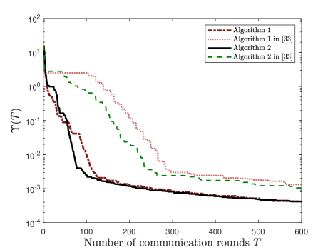
Figure 1: Evolutions of $\Upsilon(T)$ with respect to the number of iterations of different compressed distributed algorithms with the norm-sign compressor.

From Fig. 1, when utilizing the same norm-sign compressor, it is evident that the proposed Algorithms 1 and 2 demonstrate faster convergence speeds compared to Algorithm 1 and 2 in [33]. Moreover, Algorithm 2 exhibits a faster convergence speed than Algorithm 1, as it utilizes error feedback to correct the bias induced by biased compressors.

(ii) For the compressor with globally absolute compression errors, we choose the classical compressor: Standard uniform quantizer, and its mathematical model is as follows:

$$\mathcal{C}(X)=\Delta\lfloor\frac{X}{\Delta}+\frac{\mathbf{1}_{d}}{2}\rfloor,$$

where this compressor satisfies Assumption 5 with $p=\infty$ and $C=0.25\Delta^{2}$, as demonstrated in [33]. In this section, we select $\Delta=2$. The algorithm parameters for comparison are set as follows.
$\bullet$ Algorithm 3 with $\eta=0.4$, and $\gamma=0.6$.
$\bullet$ Algorithm 3 in [33] with $\eta=0.25$, $\alpha=0.1$, and $\beta=0.1$.

Fig. 2 depicts the evolution of $\Upsilon(T)$ in relation to the number of iterations $k$ for the different compressed distributed algorithms.

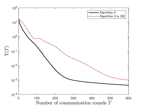
Figure 2: Evolutions of $\Upsilon(T)$ with respect to the number of iterations of different compressed distributed algorithms with the standard uniform quantizer.

From Fig.2, when utilizing the same standard uniform quantizer, it is evident that the proposed Algorithm 3 presents faster convergence compared to Algorithm 3 in [33].

(iii) For the compressor with the locally absolute compression errors. We select the classical compressor: 1-bit binary quantizer, and the mathematical model is as follows:

$$\mathcal{C}[X]=(q[X_{1}],\ldots,q[X_{d}]),$$

and

$$q[a] =\left\{\begin{aligned} &0.5,~{}a\geq 0,\\ &-0.5,~{}\text{otherwise},\end{aligned}\right.$$

where this compressor satisfies Assumption 6 with $p=\infty$ and $\psi=0.5$. The algorithm parameters for comparison are set as follows.
$\bullet$ Algorithm 3 with $\eta=0.4$, and $\gamma=0.6$.
$\bullet$ Algorithm 3 in [33] with $\eta=0.25$, $\alpha=0.1$, and $\beta=0.1$.

Fig. 3 illustrates the evolution of $\Upsilon(T)$ with respect to the number of iterations $k$ for the different compressed distributed algorithms.

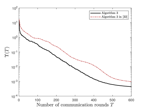
Figure 3: Evolutions of $\Upsilon(T)$ with respect to the number of iterations of different compressed distributed algorithms with the 1-bit binary quantizer.

From Fig.3, when utilizing the same 1-bit quantizer, it is evident that the proposed Algorithm 3 demonstrates fast convergence speeds compared to Algorithm 3 in [33].

To compare the transmitted bits and $\mathcal{P}$ (percentage of the number of bits transmitted by the DGT algorithm proposed in [11]) for various algorithms and compressor combinations, achieving $\Upsilon(k)\leq 10^{-3}$, Table I is provided. This table presents a comparison of transmitted bits and $\mathcal{P}$ for different algorithms and compressor combinations, ensuring that $\Upsilon(k)\leq 10^{-3}$. The experiment employs the proposed algorithm parameters outlined in (i)–(iii) and the DGT algorithm with $\eta=0.8$ and $\gamma=0.3$. For the norm-sign compressor, transmitting one variable requires $2d+b_{C}$ bits if a scalar can be transmitted with $b_{C}$ bits with adequate precision. Here, we choose $b_{C}=64$. In the case of the standard uniform quantizer, transmitting one variable demands $db_{Q}$ bits if $b_{Q}$ bits are allocated to transmit an integer; here, we set $b_{Q}=4$. As for the 1-bit binary quantizer, transmitting one variable necessitates $d$ bits. Table I demonstrates that our algorithms require significantly fewer bits compared to the DGT algorithm to achieve a specific error level. Notably, the 1-bit binary quantizer uses only 5.97% of the bits required by the DGT algorithm to achieve the same level of error.

TABLE I: Transmitted bits for different algorithms and compressors to reach $\Upsilon(T)\leq 10^{-3}$.

Algorithm	Compressor	Transmitted Bits	$\mathcal{P}$
Algorithm 1	Norm–sign compressor	74784	10.34%
Algorithm 2	Norm-sign compressor	140384	19.41%
Algorithm 3	Standard uniform quantizer	115600	15.98%
Algorithm 3	1-bit binary quantizer	43200	5.97%
Algorithm 1 [33]	Norm–sign compressor	112504	15.56%
Algorithm 2 [33]	Norm-sign compressor	183024	25.31%
Algorithm 3 [33]	Standard uniform quantizer	118200	16.35%
Algorithm 3 [33]	1-bit binary quantizer	29200	4.04%
DGT [11]	-	723200	-

VI Conclusions

In this paper, we introduced three classes of compressors to reduce the communication overhead. By integrating them with DGT algorithm, we then proposed three distributed algorithms with compressed communication for distributed nonconvex optimization. For the case where local cost functions are smooth, we designed several Lyapunov functions to demonstrate that the proposed algorithms sublinearly converge to a stationary point. Moreover, when the global cost function satisfies the P–Ł condition, we demonstrated that the proposed algorithm converges linearly to a global optimal point. One future direction is to investigate general unbalanced directed graphs.

A. Useful Lemmas

The following lemmas are used in the proofs.

Denote $\bm{B}=\mathrm{col}(B_{1},\ldots,B_{n})$, $\bm{D}=\mathrm{col}(D_{1},\ldots,D_{n})$, and $\bm{W}=W\otimes\bm{\mathrm{I}}_{d}$. Then, the compact form of the Algorithm 1 is

$$\bm{A}(k+1) =\bm{A}(k)+\varphi_{X}\bm{Q}^{X}(k),$$ (34a)

$$\bm{B}(k+1) =\bm{B}(k)+\varphi_{X}(\bm{Q}^{X}(k)-\bm{W}\bm{Q}^{X}(k)),$$ (34b)

$$\bm{C}(k+1) =\bm{C}(k)+\varphi_{Y}\bm{Q}^{Y}(k),$$ (34c)

$$\bm{D}(k+1) =\bm{D}(k)+\varphi_{Y}(\bm{Q}^{Y}(k)-\bm{W}\bm{Q}^{Y}(k)),$$ (34d)

$$\bm{X}(k+1) =\bm{X}(k)-\gamma(\bm{B}(k)+(\bm{\mathrm{I}}_{nd}-\bm{W})\bm{Q}^{X}(k))-\eta\bm{Y}(k),$$ (34e)

$$\bm{Y}(k+1) =\bm{Y}(k)-\gamma(\bm{D}(k)+(\bm{\mathrm{I}}_{nd}-\bm{W})\bm{Q}^{Y}(k))$$

$$\quad+\nabla\tilde{F}(\bm{X}(k+1))-\nabla\tilde{F}(\bm{X}(k)),$$ (34f)

$$\bm{Q}^{X}(k+1) =\mathcal{C}(\bm{X}(k+1)-\bm{A}(k+1)),$$ (34g)

$$\bm{Q}^{Y}(k+1) =\mathcal{C}(\bm{Y}(k+1)-\bm{C}(k+1)),$$ (34h)

where $\nabla\tilde{F}(\bm{X}(k))=[\nabla F^{T}_{1}(X_{1}(k)),\dots,\nabla F^{T}_{n}(X_{n}(k))]^{T}$.

For all $i\in[n]$, noted that $A_{i}(0)=B_{i}(0)=C_{i}(0)=D_{i}(0)=\bm{0}_{d}$, by mathematical induction, it is straightforward to check that $\bm{B}(k)=(\bm{\mathrm{I}}_{nd}-\bm{W})\bm{A}(k)$, and $\bm{D}(k)=(\bm{\mathrm{I}}_{nd}-\bm{W})\bm{C}(k)$.

We denote

$$\hat{\bm{X}}(k) =\bm{A}(k)+\bm{Q}^{X}(k),$$ (35a)

$$\hat{\bm{Y}}(k) =\bm{C}(k)+\bm{Q}^{Y}(k),$$ (35b)

then, (34e) and (34f) respectively can be rewritten as

$$\bm{X}(k+1) =\bm{X}(k)-\gamma(\bm{\mathrm{I}}_{nd}-\bm{W})\bm{\hat{X}}(k)-\eta\bm{Y}(k),$$ (36a)

$$\bm{Y}(k+1) =\bm{Y}(k)-\gamma(\bm{\mathrm{I}}_{nd}-\bm{W})\bm{\hat{Y}}(k)+\nabla\tilde{F}(\bm{X}(k+1))-\nabla\tilde{F}(\bm{X}(k)).$$ (36b)

If replacing $\bm{\hat{X}}(k)$ and $\hat{\bm{Y}}(k)$ in (36), then the DGT algorithm proposed in [11, 12, 47, 22, 21] is derived.

Lemma 1.

Suppose Assumption 1 holds, then for all $\omega\in\mathbb{R}^{nd}$ and $\bar{\omega}=\bm{H}\omega$, we have

$$\|(\bm{\mathrm{I}}_{nd}+\gamma(\bm{W}-\bm{\mathrm{I}}_{nd}))(\omega-\bar{\omega})\|$$

$$=\|(\bm{\mathrm{I}}_{nd}+\gamma(\bm{W}-\bm{\mathrm{I}}_{nd})-\gamma\bm{H})(\omega-\bar{\omega})\|$$

$$\leq\|(\bm{\mathrm{I}}_{nd}-\gamma\bm{\mathrm{I}}_{nd})(\omega-\bar{\omega})\|+\|\gamma(\bm{W}-\bm{H})(\omega-\bar{\omega})\|$$

$$\leq(1-\gamma)\|\omega-\bar{\omega}\|+\sigma\gamma\|\omega-\bar{\omega}\|=\delta\|\omega-\bar{\omega}\|,$$ (37)

where the first equality holds due to $\bm{H}\omega=\bm{H}\bar{\omega}$; and the second inequality holds due to $\gamma\in(0,1)$.

Lemma 2.

The following equalities hold:

$$\bar{\bm{X}}(k+1) =\bm{H}\bm{X}(k+1)$$

$$=\bm{H}(\bm{X}(k)-\gamma(\bm{\mathrm{I}}_{nd}-\bm{W})\hat{\bm{X}}(k)-\eta\bm{Y}(k))$$

$$=\bar{\bm{X}}(k)-\eta\bar{\bm{Y}}(k),$$ (38)

where the second equality holds due to (36a); and the last equality holds due to $\bm{H}(\bm{\mathrm{I}}_{nd}-\bm{W})=\bm{0}_{nd}$.

$$\bar{\bm{Y}}(k+1)= \bm{H}\bm{Y}(k+1)$$

$$= \bm{H}(\bm{Y}(k)-\gamma(\bm{\mathrm{I}}_{nd}-\bm{W})\hat{\bm{Y}}(k)+\bm{g}(k+1)-\bm{g}(k))$$

$$= \bar{\bm{g}}(k+1),$$ (39)

where $\bm{g}(k)=\nabla\tilde{F}(\bm{X}(k))$, $\tilde{F}(\bm{X})=\sum_{i=1}^{n}F_{i}(X_{i})$, and $\bar{\bm{g}}(k)=\bm{H}\bm{g}(k)$; the second equality holds due to (36b); the last equality holds due to $\bm{H}(\bm{\mathrm{I}}_{nd}-\bm{W})=\bm{0}_{nd}$ and $\bm{Y}(0)=\nabla\tilde{F}(\bm{X}(0))$.

B. Proof of Theorem 1

For the $\|\bm{X}(k+1)-\bar{\bm{X}}(k+1)\|$, we have

$$\|\bm{X}(k+1)-\bar{\bm{X}}(k+1)\|^{2}$$

$$=\|\bm{X}(k)-\gamma(\bm{\mathrm{I}}_{nd}-\bm{W})\bm{\hat{X}}(k)-\eta\bm{Y}(k)-(\bar{\bm{X}}(k)-\eta\bar{\bm{Y}}(k))\|^{2}$$

$$=\|\gamma(\bm{\mathrm{I}}_{nd}-\bm{W})(\bm{X}(k)-\bm{\hat{X}}(k))+(\bm{\mathrm{I}}_{nd}+\gamma(\bm{W}-\bm{\mathrm{I}}_{nd}))\bm{X}(k)-\bar{\bm{X}}(k)-\eta(\bm{Y}(k)-\bar{\bm{Y}}(k))\|^{2}$$

$$=\|\gamma(\bm{\mathrm{I}}_{nd}-\bm{W})(\bm{X}(k)-\bm{\hat{X}}(k))+(\bm{\mathrm{I}}_{nd}+\gamma(\bm{W}-\bm{\mathrm{I}}_{nd}))(\bm{X}(k)-\bar{\bm{X}}(k))-\eta(\bm{Y}(k)-\bar{\bm{Y}}(k))\|^{2}$$

$$\leq(2\gamma\|\bm{X}(k)-\bm{\hat{X}}(k)\|+\delta\|\bm{X}(k)-\bar{\bm{X}}(k)\|+\eta\|\bm{Y}(k)-\bar{\bm{Y}}(k)\|)^{2}$$

$$\leq\frac{8\gamma}{1-\sigma}\|\bm{X}(k)-\bm{\hat{X}}(k)\|^{2}+\delta\|\bm{X}(k)-\bar{\bm{X}}(k)\|^{2}+\frac{2\eta^{2}}{\gamma(1-\sigma)}\|\bm{Y}(k)-\bar{\bm{Y}}(k)\|^{2},$$ (40)

where the first equality holds due to (36a) and (2); the second equality holds due to (2); the last equality holds due to $(\bm{W}-\bm{\mathrm{I}}_{nd})\bm{H}=\bm{0}_{nd}$; the first inequality holds due to (1); and the last inequality holds due to the Cauchy–Schwarz inequality.

Based on (5), (34g) and (35a), we have

$$\bm{\mathrm{E}}_{\mathcal{C}}[\|\bm{X}(k)-\hat{\bm{X}}(k)\|^{2}]=\bm{\mathrm{E}}_{\mathcal{C}}[\|\bm{X}(k)-\bm{A}(k)-\mathcal{C}(\bm{X}(k)-\bm{A}(k))\|^{2}]\leq C\|\bm{X}(k)-\bm{A}(k)\|^{2}.$$ (41)

From (Compressed Gradient Tracking Algorithms for Distributed Nonconvex Optimization) and (41), we have

$$\bm{\mathrm{E}}_{\mathcal{C}}[\|\bm{X}(k+1)-\bar{\bm{X}}(k+1)\|^{2}]$$

$$\leq\bm{\mathrm{E}}_{\mathcal{C}}[\delta\|\bm{X}(k)-\bar{\bm{X}}(k)\|^{2}+\frac{2\eta^{2}}{\gamma(1-\sigma)}\|\bm{Y}(k)-\bar{\bm{Y}}(k)\|^{2}+\frac{8\gamma}{1-\sigma}C\|\bm{X}(k)-\bm{A}(k)\|^{2}],$$ (42)

where the inequality holds due to the Cauchy–Schwarz inequality.

For the $\|\bm{Y}(k+1)-\bar{\bm{Y}}(k+1)\|$, we have

$$\|\bm{Y}(k+1)-\bar{\bm{Y}}(k+1)\|^{2}$$

$$=\|\bm{Y}(k)-\gamma(\bm{\mathrm{I}}_{nd}-\bm{W})\bm{\hat{Y}}(k)+\bm{g}(k+1)-\bm{g}(k)-\bar{\bm{g}}(k+1)\|^{2}$$

$$=\|\gamma(\bm{\mathrm{I}}_{nd}-\bm{W})(\bm{Y}(k)-\bm{\hat{Y}}(k))+(\bm{\mathrm{I}}_{nd}+\gamma(\bm{W}-\bm{\mathrm{I}}_{nd}))$$

$$\quad\times(\bm{Y}(k)-\bar{\bm{Y}}(k))+\bm{g}(k+1)-\bm{g}(k)-\bar{\bm{g}}(k+1)+\bar{\bm{g}}(k)\|^{2}$$

$$=\|\gamma(\bm{\mathrm{I}}_{nd}-\bm{W})(\bm{Y}(k)-\bm{\hat{Y}}(k))+(\bm{\mathrm{I}}_{nd}+\gamma(\bm{W}-\bm{\mathrm{I}}_{nd}))$$

$$\quad\times(\bm{Y}(k)-\bar{\bm{Y}}(k))+(\bm{\mathrm{I}}_{nd}-\bm{H})(\bm{g}(k+1)-\bm{g}(k))\|^{2}$$

$$\leq(2\gamma\|\bm{Y}(k)-\bm{\hat{Y}}(k)\|+\delta\|\bm{Y}(k)-\bar{\bm{Y}}(k)\|+\bm{L}_{f}\|\bm{X}(k+1)-\bm{X}(k)\|)^{2}$$

$$\leq\frac{8\gamma}{1-\sigma}\|\bm{Y}(k)-\bm{\hat{Y}}(k)\|^{2}+\delta\|\bm{Y}(k)-\bar{\bm{Y}}(k)\|^{2}+\frac{2L_{f}^{2}}{\gamma(1-\sigma)}\|\bm{X}(k+1)-\bm{X}(k)\|^{2},$$ (43)

where the first equality holds due to (36b); the second equality holds due to $(\bm{W}-\bm{\mathrm{I}}_{nd})\bm{H}=\bm{0}_{nd}$; the last equality holds due to (2); the first inequality holds due to (2), (1), and $\rho(\bm{\mathrm{I}}_{nd}-\bm{H})\leq 1$; the last inequality holds due to (2) and the Cauchy–Schwarz inequality.

Denote $\bm{g}^{0}(k)=\nabla\tilde{F}(\bar{\bm{X}}(k))$, and $\bar{\bm{g}}^{0}(k)=\bm{H}\bm{g}^{0}(k)=\bm{1}_{n}\otimes\nabla F(\bar{X}(k))$. Then, from Assumption 2 and $\rho(\bm{H})=1$, we have

$$\|\bar{\bm{g}}^{0}(k)-\bar{\bm{g}}(k)\|=\|\bm{H}(\bm{g}^{0}(k)-\bm{g}(k))\leq\|\bm{g}^{0}(k)-\bm{g}(k)\|\leq L_{f}\|\bm{X}(k)-\bar{\bm{X}}(k)\|.$$ (44)

Based on (36a), (2), and (44), it can be obtained that

$$\|\bm{X}(k+1)-\bm{X}(k)\|$$

$$=\|\bm{X}(k)-\gamma(\bm{\mathrm{I}}_{nd}-\bm{W})\bm{\hat{X}}(k)-\eta\bm{Y}(k)-\bm{X}(k)\|$$

$$=\|\gamma(\bm{\mathrm{I}}_{nd}-\bm{W})(\bm{X}(k)-\bm{\hat{X}}(k))+\gamma(\bm{W}-\bm{\mathrm{I}}_{nd})(\bm{X}(k)-\bar{\bm{X}}(k))-\eta(\bm{Y}(k)-\bar{\bm{Y}}(k))$$

$$\quad+\eta(\bar{\bm{g}}^{0}(k)-\bar{\bm{g}}(k))-\eta\bar{\bm{g}}^{0}(k)\|$$

$$\leq 2\gamma\|\bm{X}(k)-\bm{\hat{X}}(k)\|+(2\gamma+\eta L_{f})\|\bm{X}(k)-\bar{\bm{X}}(k)\|+\eta\|\bm{Y}(k)-\bar{\bm{Y}}(k)\|+\eta\|\bar{\bm{g}}^{0}(k)\|,$$ (45)

where the second equality holds due to $(\bm{W}-\bm{\mathrm{I}}_{nd})\bm{H}=\bm{0}_{nd}$.

Based on (5), (34h) and (35b), it can be calculated that

$$\bm{\mathrm{E}}_{\mathcal{C}}[\|\bm{Y}(k)-\hat{\bm{Y}}(k)\|^{2}]=\bm{\mathrm{E}}_{\mathcal{C}}[\|\bm{Y}(k)-\bm{C}(k)-\mathcal{C}(\bm{Y}(k)-\bm{C}(k))\|^{2}]\leq C\|\bm{Y}(k)-\bm{C}(k)\|^{2}.$$ (46)

From (41), (Compressed Gradient Tracking Algorithms for Distributed Nonconvex Optimization), (Compressed Gradient Tracking Algorithms for Distributed Nonconvex Optimization), and (46), we have

$$\bm{\mathrm{E}}_{\mathcal{C}}[\|\bm{Y}(k+1)-\bar{\bm{Y}}(k+1)\|^{2}]$$

$$\leq\bm{\mathrm{E}}_{\mathcal{C}}[\frac{8\gamma}{1-\sigma}\|\bm{Y}(k)-\bm{\hat{Y}}(k)\|^{2}+\delta\|\bm{Y}(k)-\bar{\bm{Y}}(k)\|^{2}+\frac{8L_{f}^{2}}{\gamma(1-\sigma)}(4\gamma^{2}\|\bm{X}(k)-\bm{\hat{X}}(k)\|^{2}$$

$$\quad+(8\gamma^{2}+2\eta^{2}L_{f}^{2})\|\bm{X}(k)-\bar{\bm{X}}(k)\|^{2}+\eta^{2}\|\bm{Y}(k)-\bar{\bm{Y}}(k)\|^{2}+\eta^{2}\|\bar{\bm{g}}^{0}(k)\|^{2})]$$

$$\leq\bm{\mathrm{E}}_{\mathcal{C}}[(\delta+\frac{8L_{f}^{2}}{\gamma(1-\sigma)}\eta^{2})\|\bm{Y}(k)-\bar{\bm{Y}}(k)\|^{2}+\frac{8L_{f}^{2}}{\gamma(1-\sigma)}(4\gamma^{2}C\|\bm{X}(k)-\bm{A}(k)\|^{2}$$

$$\quad+(8\gamma^{2}+2\eta^{2}L_{f}^{2})\|\bm{X}(k)-\bar{\bm{X}}(k)\|^{2}+\eta^{2}\|\bar{\bm{g}}^{0}(k)\|^{2})+\frac{8\gamma}{1-\sigma}C\|\bm{Y}(k)-\bm{C}(k)\|^{2}].$$ (47)

For the $\bm{\mathrm{E}}_{\mathcal{C}}[\|\bm{X}(k+1)-\bm{A}(k+1)\|^{2}]$, we have

$$\bm{\mathrm{E}}_{\mathcal{C}}[\|\bm{X}(k+1)-\bm{A}(k+1)\|^{2}]$$

$$=\bm{\mathrm{E}}_{\mathcal{C}}[\|\bm{X}(k+1)-\bm{X}(k)+\bm{X}(k)-\bm{A}(k)-\varphi_{X}\bm{Q}^{X}(k)\|^{2}]$$

$$=\bm{\mathrm{E}}_{\mathcal{C}}[\|\bm{X}(k+1)-\bm{X}(k)+(1-\varphi_{X}r)(\bm{X}(k)-\bm{A}(k))$$

$$\quad+\varphi_{X}r((\bm{X}(k)-\bm{A}(k))-\mathcal{C}_{r}(\bm{X}(k)-\bm{A}(k)))\|^{2}]$$

$$\leq\bm{\mathrm{E}}_{\mathcal{C}}[(1+c_{1}^{-1})\|\bm{X}(k+1)-\bm{X}(k)\|^{2}+(1+c_{1})(1-\varphi_{X}r)\|\bm{X}(k)-\bm{A}(k)\|^{2}$$

$$\quad+(1+c_{1})\varphi_{X}r\|\bm{X}(k)-\bm{A}(k)-\mathcal{C}_{r}(\bm{X}(k)-\bm{A}(k))\|^{2}]$$

$$\leq\bm{\mathrm{E}}_{\mathcal{C}}[(1+c_{1}^{-1})\|\bm{X}(k+1)-\bm{X}(k)\|^{2}+(1+c_{1})(1-\varphi_{X}r)\|\bm{X}(k)-\bm{A}(k)\|^{2}$$

$$\quad+(1+c_{1})\varphi_{X}r(1-\psi)\|\bm{X}(k)-\bm{A}(k)\|^{2}]$$

$$=\bm{\mathrm{E}}_{\mathcal{C}}[(1+c_{1}^{-1})\|\bm{X}(k+1)-\bm{X}(k)\|^{2}+(1-c_{1}-2c_{1}^{2})\|\bm{X}(k)-\bm{A}(k)\|^{2}]$$

$$\leq\bm{\mathrm{E}}_{\mathcal{C}}[(1+c_{1}^{-1})(2\gamma\|\bm{X}(k)-\bm{\hat{X}}(k)\|+(2\gamma+\eta L_{f})\|\bm{X}(k)-\bar{\bm{X}}(k)\|+\eta\|\bm{Y}(k)-\bar{\bm{Y}}(k)\|$$

$$\quad+\eta\|\bar{\bm{g}}^{0}(k)\|)^{2}+(1-c_{1}-2c_{1}^{2})\|\bm{X}(k)-\bm{A}(k)\|^{2}]$$

$$\leq\bm{\mathrm{E}}_{\mathcal{C}}[4(1+c_{1}^{-1})(4\gamma^{2}C\|\bm{X}(k)-\bm{A}(k)\|^{2}+(8\gamma^{2}+2\eta^{2}L_{f}^{2})\|\bm{X}(k)-\bar{\bm{X}}(k)\|^{2}$$

$$\quad+\eta^{2}\|\bm{Y}(k)-\bar{\bm{Y}}(k)\|^{2}+\eta^{2}\|\bar{\bm{g}}^{0}(k)\|^{2})+(1-c_{1}-2c_{1}^{2})\|\bm{X}(k)-\bm{A}(k)\|^{2}],$$ (48)

where $\mathcal{C}_{r}(\cdot)=\frac{\mathcal{C}(\cdot)}{r}$; the first and second equalities hold due to (34); the first inequality holds due to the Cauchy–Schwarz inequality; the second inequality holds due to (4); the third inequality holds due to (Compressed Gradient Tracking Algorithms for Distributed Nonconvex Optimization); the last inequality holds due to (41), and the Cauchy–Schwarz inequality.

For the $\bm{\mathrm{E}}_{\mathcal{C}}[\|\bm{Y}(k+1)-\bm{C}(k+1)\|^{2}]$, we have

$$\bm{\mathrm{E}}_{\mathcal{C}}[\|\bm{Y}(k+1)-\bm{C}(k+1)\|^{2}]$$

$$=\bm{\mathrm{E}}_{\mathcal{C}}[\|\bm{Y}(k+1)-\bm{Y}(k)+\bm{Y}(k)-\bm{C}(k)-\varphi_{Y}\bm{Q}^{Y}(k)\|^{2}]$$

$$=\bm{\mathrm{E}}_{\mathcal{C}}[\|\bm{Y}(k+1)-\bm{Y}(k)+(1-\varphi_{Y}r)(\bm{Y}(k)-\bm{C}(k))$$

$$\quad+\varphi_{Y}r((\bm{Y}(k)-\bm{C}(k))-\mathcal{C}_{r}(\bm{Y}(k)-\bm{C}(k)))\|^{2}]$$

$$\leq\bm{\mathrm{E}}_{\mathcal{C}}[(1+c_{2}^{-1})\|\bm{Y}(k+1)-\bm{Y}(k)\|^{2}+(1+c_{2})(1-\varphi_{Y}r)\|\bm{Y}(k)-\bm{C}(k)\|^{2}$$

$$\quad+(1+c_{2})\varphi_{Y}r\|\bm{Y}(k)-\bm{C}(k)-\mathcal{C}_{r}(\bm{Y}(k)-\bm{C}(k))\|^{2}]$$

$$\leq\bm{\mathrm{E}}_{\mathcal{C}}[(1+c_{2}^{-1})\|\bm{Y}(k+1)-\bm{Y}(k)\|^{2}+(1+c_{2})(1-\varphi_{Y}r)\|\bm{Y}(k)-\bm{C}(k)\|^{2}$$

$$\quad+(1+c_{2})\varphi_{Y}r(1-\psi)\|\bm{Y}(k)-\bm{C}(k)\|^{2}]$$

$$=\bm{\mathrm{E}}_{\mathcal{C}}[(1+c_{2}^{-1})\|\bm{Y}(k+1)-\bm{Y}(k)\|^{2}+(1-c_{2}-2c_{2}^{2})\|\bm{Y}(k)-\bm{C}(k)\|^{2}],$$ (49)

where the first equality holds due to (34c); the second equality holds due to (34h); the first inequality holds due to the Cauchy–Schwarz inequality; and the last inequality holds due to (4).

Based on (36b), (44) and (Compressed Gradient Tracking Algorithms for Distributed Nonconvex Optimization), it can be derived that

$$\|\bm{Y}(k+1)-\bm{Y}(k)\|$$

$$=\|\bm{Y}(k)-\gamma(\bm{\mathrm{I}}_{nd}-\bm{W})\bm{\hat{Y}}(k)+\bm{g}(k+1)-\bm{g}(k)-\bm{Y}(k)\|$$

$$=\|\gamma(\bm{\mathrm{I}}_{nd}-\bm{W})(\bm{Y}(k)-\bm{\hat{Y}}(k))+\gamma(\bm{W}-\bm{\mathrm{I}}_{nd})(\bm{Y}(k)-\bar{\bm{Y}}(k))+\bm{g}(k+1)-\bm{g}(k)\|$$

$$\leq 2\gamma\|\bm{Y}(k)-\bm{\hat{Y}}(k)\|+2\gamma\|\bm{Y}(k)-\bar{\bm{Y}}(k)\|+L_{f}\|\bm{X}(k+1)-\bm{X}(k)\|$$

$$\leq 2\gamma\|\bm{Y}(k)-\bm{\hat{Y}}(k)\|+(2\gamma+\eta L_{f})\|\bm{Y}(k)-\bar{\bm{Y}}(k)\|+L_{f}(2\gamma\|\bm{X}(k)-\bm{\hat{X}}(k)\|$$

$$\quad+(2\gamma+\eta L_{f})\|\bm{X}(k)-\bar{\bm{X}}(k)\|+\eta\|\bar{\bm{g}}^{0}(k)\|),$$ (50)

where the last equality holds due to $(\bm{W}-\bm{\mathrm{I}}_{nd})\bm{H}=\bm{0}_{nd}$ and (2).

From (Compressed Gradient Tracking Algorithms for Distributed Nonconvex Optimization) and (Compressed Gradient Tracking Algorithms for Distributed Nonconvex Optimization), we have

$$\bm{\mathrm{E}}_{\mathcal{C}}[\|\bm{Y}(k+1)-\bm{C}(k+1)\|^{2}]$$

$$\leq\bm{\mathrm{E}}_{\mathcal{C}}[(1+c_{2}^{-1})(2\gamma\|\bm{Y}(k)-\bm{\hat{Y}}(k)\|+(2\gamma+\eta L_{f})\|\bm{Y}(k)-\bar{\bm{Y}}(k)\|$$

$$\quad+L_{f}(2\gamma\|\bm{X}(k)-\bm{\hat{X}}(k)\|+(2\gamma+\eta L_{f})\|\bm{X}(k)-\bar{\bm{X}}(k)\|+\eta\|\bar{\bm{g}}^{0}(k)\|))^{2}$$

$$\quad+(1-c_{2}-2c_{2}^{2})\|\bm{Y}(k)-\bm{C}(k)\|^{2}]$$

$$\leq\bm{\mathrm{E}}_{\mathcal{C}}[5(1+c_{2}^{-1})(4\gamma^{2}C\|\bm{Y}(k)-\bm{C}(k)\|^{2}+(8\gamma^{2}+2\eta^{2}L_{f}^{2})\|\bm{Y}(k)-\bar{\bm{Y}}(k)\|^{2}$$

$$\quad+L_{f}^{2}(4\gamma^{2}C\|\bm{X}(k)-\bm{A}(k)\|^{2}+(8\gamma^{2}+2\eta^{2}L_{f}^{2})\|\bm{X}(k)-\bar{\bm{X}}(k)\|^{2}+\eta^{2}\|\bar{\bm{g}}^{0}(k)\|^{2}))$$

$$\quad+(1-c_{2}-2c_{2}^{2})\|\bm{Y}(k)-\bm{C}(k)\|^{2}],$$ (51)

where the last inequality holds due to (41), (46), and the Cauchy–Schwarz inequality.

From [48, Lemma 1.2.3], we know that (2) implies

$$|F_{i}(Y)-F_{i}(X)-(Y-X)^{T}\nabla F_{i}(X)|\leq\frac{L_{f}}{2}\|Y-X\|^{2},~{}\forall X,~{}Y\in\mathbb{R}^{d}.$$ (52)

For the $n(F(\bar{X}(k+1)-F^{\star}))$, based on (52), we have

$$n(F(\bar{X}(k+1))-F^{\star})$$

$$=n(F(\bar{X}(k))-F^{\star}+F(\bar{X}(k+1))-F(\bar{X}(k)))$$

$$\leq n(F(\bar{X}(k))-F^{\star})-\eta\bar{\bm{g}}^{T}(k)\bm{g}^{0}(k)+\frac{\eta^{2}L_{f}}{2}\|\bar{\bm{g}}(k)\|^{2}$$

$$=n(F(\bar{X}(k))-F^{\star})-\eta\bar{\bm{g}}^{T}(k)\bar{\bm{g}}^{0}(k)+\frac{\eta^{2}L_{f}}{2}\|\bar{\bm{g}}(k)\|^{2}$$

$$=n(F(\bar{X}(k))-F^{\star})-\frac{\eta}{2}\bar{\bm{g}}^{T}(k)(\bar{\bm{g}}(k)+\bar{\bm{g}}^{0}(k)-\bar{\bm{g}}(k))$$

$$\quad-\frac{\eta}{2}(\bar{\bm{g}}(k)+\bar{\bm{g}}^{0}(k)-\bar{\bm{g}}^{0}(k))^{T}\bar{\bm{g}}^{0}(k)+\frac{\eta^{2}L_{f}}{2}\|\bar{\bm{g}}(k)\|^{2}$$

$$\leq n(F(\bar{X}(k))-F^{\star})-\frac{\eta}{4}\|\bar{\bm{g}}(k)\|^{2}+\frac{\eta}{4}\|\bar{\bm{g}}^{0}(k)-\bar{\bm{g}}(k)\|^{2}$$

$$\quad-\frac{\eta}{4}\|\bar{\bm{g}}^{0}(k)\|^{2}+\frac{\eta}{4}\|\bar{\bm{g}}^{0}(k)-\bar{\bm{g}}(k)\|^{2}+\frac{\eta^{2}L_{f}}{2}\|\bar{\bm{g}}(k)\|^{2}$$

$$\leq n(F(\bar{X}(k))-F^{\star})-\frac{\eta}{4}(1-2\eta L_{f})\|\bar{\bm{g}}(k)\|^{2}$$

$$\quad+\frac{\eta}{2}L_{f}^{2}\|\bm{X}(k)-\bar{\bm{X}}(k)\|^{2}-\frac{\eta}{4}\|\bar{\bm{g}}^{0}(k)\|^{2},$$ (53)

where the first inequality holds since that $F$ is smooth and (52); the second equality holds due to $\bar{\bm{g}}^{T}(k)\bm{g}^{0}(k)=\bm{g}^{T}(k)\bm{H}\bm{g}^{0}(k)=\bm{g}^{T}(k)\bm{H}\bm{H}\bm{g}^{0}(k)=\bar{\bm{g}}^{T}(k)\bar{\bm{g}}^{0}(k)$; the second inequality holds due to the Cauchy–Schwarz inequality; and the last inequality holds due to (44).

From (Compressed Gradient Tracking Algorithms for Distributed Nonconvex Optimization), (Compressed Gradient Tracking Algorithms for Distributed Nonconvex Optimization), (Compressed Gradient Tracking Algorithms for Distributed Nonconvex Optimization), (Compressed Gradient Tracking Algorithms for Distributed Nonconvex Optimization), we have

$$\bm{\mathrm{E}}_{\mathcal{C}}[U(k+1)]$$

$$\leq\bm{\mathrm{E}}_{\mathcal{C}}[\theta_{5}\|\bm{X}(k)-\bar{\bm{X}}(k)\|^{2}+\theta_{6}\|\bm{Y}(k)-\bar{\bm{Y}}(k)\|^{2}+\theta_{7}\|\bm{X}(k)-\bm{A}(k)\|^{2}$$

$$\quad+\theta_{8}\|\bm{Y}(k)-\bm{C}(k)\|^{2}+n(F(\bar{X}(k))-F^{\star})-\theta_{2}\|\bar{\bm{g}}^{0}(k)\|^{2}-\theta_{9}\|\bar{\bm{g}}(k)\|^{2}],$$ (54)

where

$$\theta_{5} =\delta+\phi\xi_{1}+\xi_{2}+\xi_{3}+\frac{\eta L_{f}^{2}}{2},~{}\theta_{6}=\xi_{4}+\phi\xi_{5}+\xi_{6}+\xi_{7},$$

$$\theta_{7} =\xi_{8}+\phi\xi_{9}+\xi_{10}+\xi_{11},~{}\theta_{8}=\phi\xi_{8}+\xi_{12},~{}\theta_{9}=\frac{\eta}{4}(1-2\eta L_{f}),$$

$$\xi_{1} =\frac{8L_{f}^{2}}{(1-\sigma)\gamma}(8\gamma^{2}+2\eta^{2}L_{f}^{2}),~{}\xi_{2}=4(8\gamma^{2}+2\eta^{2}L_{f}^{2})(1+c_{1}^{-1}),~{}\xi_{3}=\xi_{7}L_{f}^{2},$$

$$\xi_{4} =\frac{2\eta^{2}}{\gamma(1-\sigma)},~{}\xi_{5}=\delta+\frac{8L_{f}^{2}}{(1-\sigma)\gamma}\eta^{2},~{}\xi_{6}=4(1+c_{1}^{-1})\eta^{2},$$

$$\xi_{7} =5(1+c_{2}^{-1})(8\gamma^{2}+2\eta^{2}L_{f}^{2}),~{}\xi_{8}=\frac{8\gamma}{1-\sigma}C,$$

$$\xi_{9} =\frac{32L_{f}^{2}}{1-\sigma}\gamma C,~{}\xi_{10}=16\gamma^{2}(1+c_{1}^{-1})C+(1-c_{1}-2c_{1}^{2}),$$

$$\xi_{11} =5(1+c_{2}^{-1})4\gamma^{2}L_{f}^{2}C,~{}\xi_{12}=20\gamma^{2}(1+c_{2}^{-1})C+(1-c_{2}-2c_{2}^{2}).$$

Next, we prove that $\theta_{5},~{}\theta_{6},~{}\theta_{7},~{}\theta_{8}\in(0,1)$, $\theta_{2},~{}\theta_{9}\geq 0$.

(i) We first prove that the following inequality holds.

$$0<\theta_{5}<1-0.37(1-\sigma)\gamma<1.$$ (55)

From $\eta<\frac{(1-\sigma)^{2}\gamma}{40L_{f}}$, we have

$$\phi\xi_{1}<\frac{(1-\sigma)^{2}}{320L_{f}^{2}}\frac{64.01L_{f}^{2}\gamma^{2}}{(1-\sigma)\gamma}<0.21(1-\sigma)\gamma.$$ (56)

From $\gamma<\frac{1-\sigma}{160(1+c_{1}^{-1})}$, and $\eta<\frac{(1-\sigma)^{2}\gamma}{40L_{f}}$, we have

$$\xi_{2}<\frac{32.005(1-\sigma)}{160(1+c_{1}^{-1})}\gamma(1+c_{1}^{-1})<0.21(1-\sigma)\gamma.$$ (57)

From $\gamma<\frac{1-\sigma}{40000(1+c_{2}^{-1})L_{f}^{2}}$, and $\eta<\frac{(1-\sigma)^{2}\gamma}{40L_{f}}$, we have

$$\xi_{3}<40.00625\gamma^{2}L_{f}^{2}<0.0011(1-\sigma)\gamma.$$ (58)

From $\eta<\frac{0.4(1-\sigma)\gamma}{L_{f}^{2}}$, we have

$$\eta L_{f}^{2}/2<0.2(1-\sigma)\gamma.$$ (59)

From $\gamma<\frac{1-\sigma}{160(1+c_{1}^{-1})}$, and (56)–(59), we know that (55) holds. This completes the proof.

(ii) We second prove that the following inequality holds.

$$0<\theta_{6}<\phi(1-0.07(1-\sigma)\gamma)<\phi.$$ (60)

From $\eta<\frac{(1-\sigma)^{2}\gamma}{40L_{f}}$, we have

$$\xi_{4}<\frac{2}{\gamma(1-\sigma)}\frac{(1-\sigma)^{4}\gamma^{2}}{1600L_{f}^{2}}=\frac{(1-\sigma)^{2}}{320L_{f}^{2}}\frac{2(1-\sigma)\gamma}{5}=0.4\phi(1-\sigma)\gamma.$$ (61)

From $\eta<\frac{(1-\sigma)^{2}\gamma}{40L_{f}}$, we have

$$4\phi\frac{2L_{f}^{2}}{(1-\sigma)\gamma}\eta^{2}<\phi\frac{8L_{f}^{2}}{(1-\sigma)\gamma}\frac{(1-\sigma)^{4}\gamma^{2}}{1600L_{f}^{2}}<0.005\phi(1-\sigma)\gamma.$$ (62)

From $\eta<\frac{(1-\sigma)^{2}}{80L_{f}}\sqrt{\frac{\gamma}{1+c_{1}^{-1}}}$, we have

$$\xi_{6}<4\frac{(1-\sigma)^{4}}{6400L_{f}^{2}}\frac{\gamma}{1+c_{1}^{-1}}(1+c_{1}^{-1})<0.2\phi(1-\sigma)\gamma.$$ (63)

From $\gamma<\frac{1-\sigma}{40000(1+c_{2}^{-1})L_{f}^{2}}$, and $\eta<\frac{(1-\sigma)^{2}\gamma}{40L_{f}}$, we have

$$\xi_{7}<40.00625(1+c_{2}^{-1})\gamma^{2}<\frac{(1-\sigma)^{2}}{320L_{f}^{2}}0.321(1-\sigma)\gamma=0.321\phi(1-\sigma)\gamma.$$ (64)

From $\gamma<\frac{1-\sigma}{160(1+c_{1}^{-1})}$, and (61)–(64), we know that (60) holds. This completes the proof.

(iii) We third prove that the following inequality holds.

$$0<\theta_{7}<1-0.44c_{1}(2c_{1}+1)<1.$$ (65)

From $\gamma<\frac{c_{1}(1-\sigma)}{40C}$, we have

$$\xi_{8}<\frac{8}{1-\sigma}\frac{c_{1}(1-\sigma)C}{40C}<0.2c_{1}(2c_{1}+1).$$ (66)

From $\gamma<\frac{c_{1}(1-\sigma)}{40C}$, we have

$$\phi\xi_{9}<\frac{(1-\sigma)^{2}}{320L_{f}^{2}}\frac{32L_{f}^{2}\gamma^{2}C}{(1-\sigma)\gamma}<\frac{(1-\sigma)C}{10}\frac{c_{1}(1-\sigma)}{40C}<0.0025c_{1}(2c_{1}+1).$$ (67)

From $\gamma<\frac{c_{1}}{8\sqrt{C}}$, we have

$$16\gamma^{2}(1+c_{1}^{-1})C<\frac{16c_{1}^{2}(1+c_{1}^{-1})C}{64C}<0.25c_{1}(2c_{1}+1).$$ (68)

From $\gamma<\frac{c_{1}}{10L_{f}\sqrt{C(1+c_{2}^{-1})}}$, we have

$$\xi_{11}<\frac{20(1+c_{2}^{-1})L_{f}^{2}c_{1}^{2}C}{100L_{f}^{2}C(1+c_{2}^{-1})}<0.1c_{1}(2c_{1}+1).$$ (69)

Considering that $\varphi_{X}\in(0,\frac{1}{r})$ and $\psi\in(0,1]$, we can ensure that $c_{1}=\frac{\varphi_{X}\psi r}{2}<\frac{1}{2}$. Consequently, we have $c_{1}(1+2c_{1})<1$. Based on (66)–(69), it becomes evident that (65) is satisfied. This completes the proof.

(iv) We fourth prove that the following inequality holds.

$$0<\theta_{8}<1-0.77c_{2}(2c_{2}+1)<1.$$ (70)

From $\gamma<\frac{c_{2}L_{f}^{2}}{C}$, we have

$$\phi\xi_{8}<\frac{(1-\sigma)^{2}}{320L_{f}^{2}}\frac{8c_{2}L_{f}^{2}C}{(1-\sigma)C}<0.025c_{2}(2c_{2}+1).$$ (71)

From $\gamma<\frac{c_{2}}{10\sqrt{C}}$, we have

$$20\gamma^{2}(1+c_{2}^{-1})C<20\frac{c_{2}^{2}(1+c_{2}^{-1})C}{100C}<0.2c_{2}(1+2c_{2}).$$ (72)

Considering that $\varphi_{Y}\in(0,\frac{1}{r})$ and $\psi\in(0,1]$, we can ensure that $c_{2}=\frac{\varphi_{Y}\psi r}{2}<\frac{1}{2}$. Consequently, we have $c_{2}(1+2c_{2})<1$. From (71)–(72), we know that (70) holds. This completes the proof.

(v) From $0<\eta<\min\{\frac{1-\sigma}{160(1+c_{1}^{-1})},\frac{9}{40(4(1+c_{1}^{-1})+5(1+c_{2}^{-1}))}\}$, we have

$$\theta_{2}>\eta(\frac{1}{4}-\frac{(1-\sigma)^{2}}{320L_{f}^{2}}\frac{8L_{f}^{2}}{(1-\sigma)}-\eta(4(1+c_{1}^{-1})+5(1+c_{2}^{-1}))>0.$$ (73)

(vi) From $0<\eta<\frac{1}{2L_{f}}$, we have

$$\theta_{9}=\frac{\eta}{4}(1-2\eta L_{f})>0.$$ (74)

Based on (Compressed Gradient Tracking Algorithms for Distributed Nonconvex Optimization), (55), (60), (65), (70), (73), (74), we have

$$\bm{\mathrm{E}}_{\mathcal{C}}[U(k+1)]\leq \bm{\mathrm{E}}_{\mathcal{C}}[U(k)]-\theta_{3}\bm{\mathrm{E}}_{\mathcal{C}}[V(k)]-\theta_{2}\bm{\mathrm{E}}_{\mathcal{C}}[\|\bar{\bm{g}}^{0}(k)\|^{2}],$$ (75a)

$$\leq \bm{\mathrm{E}}_{\mathcal{C}}[U(k)]-\theta_{1}\bm{\mathrm{E}}_{\mathcal{C}}[\|\bm{X}(k)-\bar{\bm{X}}(k)\|^{2}+\|\bar{\bm{g}}^{0}(k)\|^{2}].$$ (75b)

From (75b), we have

$$\sum_{t=0}^{k}\bm{\mathrm{E}}_{\mathcal{C}}[\|\bm{X}(t)-\bar{\bm{X}}(t)\|^{2}+\|\bar{\bm{g}}^{0}(t)\|^{2}]\leq\frac{U(0)}{\theta_{1}},$$ (76)

and

$$\bm{\mathrm{E}}_{\mathcal{C}}[n(F(\bar{X}(k))-F^{\star})]\leq\bm{\mathrm{E}}_{\mathcal{C}}[U(k)]<U(0).$$ (77)

Based on (76) and (77), we know that (10) and (11) hold. This completes the proof.

C. Proof of Theorem 2

From Assumption 3, we have

$$\|\bar{\bm{g}}^{0}(k)\|^{2}=n\|\nabla F(\bar{X}(k))\|^{2}\geq 2\nu n(F(\bar{X}(k))-F^{\star}).$$ (78)

Based on (78), and (75a), we have

$$\bm{\mathrm{E}}_{\mathcal{C}}[U(k+1)] \leq\bm{\mathrm{E}}_{\mathcal{C}}[U(k)]-\theta_{3}\bm{\mathrm{E}}_{\mathcal{C}}[V(k)]-2\nu n\theta_{2}\bm{\mathrm{E}}_{\mathcal{C}}[n(F(\bar{X}(k))-F^{\star})]$$

$$\leq(1-\theta_{4})\bm{\mathrm{E}}_{\mathcal{C}}[U(k)]\leq(1-\theta_{4})^{k+1}U(0),$$ (79)

where $\theta_{4}=\min\{\theta_{3},2\nu\theta_{2}\}$.

From (60), (65), and (70), we have $0<\theta_{4}\leq\theta_{3}<1$. Based on (Compressed Gradient Tracking Algorithms for Distributed Nonconvex Optimization), we know that (12) holds. This completes the proof.

D. Proof of Theorem 3

We denote

$$\hat{\bm{X}}(k)=\bm{A}(k)+\hat{\bm{Q}}^{X}(k),$$ (80)

$$\hat{\bm{Y}}(k)=\bm{C}(k)+\hat{\bm{Q}}^{Y}(k).$$ (81)

Then, the compact form of (13e) and (13f) respectively can be written as (36), since $\bm{B}(k)=(\bm{\mathrm{I}}_{nd}-\bm{W})\bm{A}(k)$ and $\bm{D}(k)=(\bm{\mathrm{I}}_{nd}-\bm{W})\bm{C}(k)$.

From (13i), (13k), and (5), we have

$$\bm{\mathrm{E}}_{\mathcal{C}}[\|\bm{E}^{X}(k+1)\|^{2}]$$

$$\leq\bm{\mathrm{E}}_{\mathcal{C}}[C\|\varsigma\bm{E}^{X}(k)+\bm{X}(k)-\bm{A}(k)\|^{2}]$$

$$\leq\bm{\mathrm{E}}_{\mathcal{C}}[2C\varsigma^{2}\|\bm{E}^{X}(k)\|^{2}+2C\|\bm{X}(k)-\bm{A}(k)\|^{2}],$$ (82)

where the last inequality holds due to the Cauchy–Schwarz inequality.

Based on (36a), (80), and (Compressed Gradient Tracking Algorithms for Distributed Nonconvex Optimization), we have

$$\bm{\mathrm{E}}_{\mathcal{C}}[\|\bm{X}(k)-\hat{\bm{X}}(k)\|^{2}]$$

$$=\bm{\mathrm{E}}_{\mathcal{C}}[\|\bm{E}^{X}(k+1)-\varsigma\bm{E}^{X}(k)\|^{2}]$$

$$\leq\bm{\mathrm{E}}_{\mathcal{C}}[2\|\bm{E}^{X}(k+1)\|^{2}+2\varsigma^{2}\|\bm{E}^{X}(k)\|^{2}]$$

$$\leq\bm{\mathrm{E}}_{\mathcal{C}}[2\varsigma^{2}(2C+1)\|\bm{E}^{X}(k)\|^{2}+4C\|\bm{X}(k)-\bm{A}(k)\|^{2}],$$ (83)

where the first inequality holds due to the Cauchy–Schwarz inequality.

Then, from (Compressed Gradient Tracking Algorithms for Distributed Nonconvex Optimization) and (Compressed Gradient Tracking Algorithms for Distributed Nonconvex Optimization), we have

$$\bm{\mathrm{E}}_{\mathcal{C}}[\|\bm{X}(k+1)-\bar{\bm{X}}(k+1)\|^{2}]$$

$$\leq\bm{\mathrm{E}}_{\mathcal{C}}[\frac{8\gamma}{1-\sigma}(2\varsigma^{2}(2C+1)\|\bm{E}^{X}(k)\|^{2}+4C\|\bm{X}(k)-\bm{A}(k)\|^{2})+\delta\|\bm{X}(k)-\bar{\bm{X}}(k)\|^{2}$$

$$\quad+\frac{2\eta^{2}}{\gamma(1-\sigma)}\|\bm{Y}(k)-\bar{\bm{Y}}(k)\|^{2}].$$ (84)

From (13j), (13l), and (5), we have

$$\bm{\mathrm{E}}_{\mathcal{C}}[\|\bm{E}^{Y}(k+1)\|^{2}]$$

$$\leq\bm{\mathrm{E}}_{\mathcal{C}}[C\|\varsigma\bm{E}^{Y}(k)+\bm{Y}(k)-\bm{C}(k)\|^{2}]$$

$$\leq\bm{\mathrm{E}}_{\mathcal{C}}[2C\varsigma^{2}\|\bm{E}^{Y}(k)\|^{2}+2C\|\bm{Y}(k)-\bm{C}(k)\|^{2}],$$ (85)

where the last inequality holds due to the Cauchy–Schwarz inequality.

Based on (36b), (81), and (Compressed Gradient Tracking Algorithms for Distributed Nonconvex Optimization), we have

$$\bm{\mathrm{E}}_{\mathcal{C}}[\|\bm{Y}(k)-\hat{\bm{Y}}(k)\|^{2}]$$

$$=\bm{\mathrm{E}}_{\mathcal{C}}[\|\bm{E}^{Y}(k+1)-\varsigma\bm{E}^{Y}(k)\|^{2}]$$

$$\leq\bm{\mathrm{E}}_{\mathcal{C}}[2\|\bm{E}^{Y}(k+1)\|^{2}+2\varsigma^{2}\|\bm{E}^{Y}(k)\|^{2}]$$

$$\leq\bm{\mathrm{E}}_{\mathcal{C}}[2\varsigma^{2}(2C+1)\|\bm{E}^{Y}(k)\|^{2}+4C\|\bm{Y}(k)-\bm{C}(k)\|^{2}],$$ (86)

where the first inequality holds due to the Cauchy–Schwarz inequality.

Then, from (Compressed Gradient Tracking Algorithms for Distributed Nonconvex Optimization), (Compressed Gradient Tracking Algorithms for Distributed Nonconvex Optimization), and (Compressed Gradient Tracking Algorithms for Distributed Nonconvex Optimization), we have

$$\bm{\mathrm{E}}_{\mathcal{C}}[\|\bm{Y}(k+1)-\bar{\bm{Y}}(k+1)\|^{2}]$$

$$\leq\bm{\mathrm{E}}_{\mathcal{C}}[\frac{8\gamma}{1-\sigma}(2\varsigma^{2}(2C+1)\|\bm{E}^{Y}(k)\|^{2}+4C\|\bm{Y}(k)-\bm{C}(k)\|^{2})+\delta\|\bm{Y}(k)-\bar{\bm{Y}}(k)\|^{2}$$

$$\quad+\frac{8L_{f}^{2}}{\gamma(1-\sigma)}(4\gamma^{2}(2\varsigma^{2}(2C+1)\|\bm{E}^{X}(k)\|^{2}+4C\|\bm{X}(k)-\bm{A}(k)\|^{2})$$

$$\quad+(8\gamma^{2}+2\eta^{2}L_{f}^{2})\|\bm{X}(k)-\bar{\bm{X}}(k)\|^{2}+\eta^{2}\|\bm{Y}(k)-\bar{\bm{Y}}(k)\|^{2}+\eta^{2}\|\bar{\bm{g}}^{0}(k)\|^{2})].$$ (87)

From (Compressed Gradient Tracking Algorithms for Distributed Nonconvex Optimization) and (Compressed Gradient Tracking Algorithms for Distributed Nonconvex Optimization), we have

$$\bm{\mathrm{E}}_{\mathcal{C}}[\|\bm{X}(k+1)-\bm{A}(k+1)\|^{2}]$$

$$\leq \bm{\mathrm{E}}_{\mathcal{C}}[4(1+c_{1}^{-1})(4\gamma^{2}\|\bm{X}(k)-\hat{\bm{X}}(k)\|^{2}+(8\gamma^{2}+2\eta^{2}L_{f}^{2})\|\bm{X}(k)-\bar{\bm{X}}(k)\|^{2}$$

$$+\eta^{2}\|\bm{Y}(k)-\bar{\bm{Y}}(k)\|^{2}+\eta^{2}\|\bar{\bm{g}}^{0}(k)\|^{2})+(1-c_{1}-2c_{1}^{2})\|\bm{X}(k)-\bm{A}(k)\|^{2}]$$

$$\leq \bm{\mathrm{E}}_{\mathcal{C}}[4(1+c_{1}^{-1})(4\gamma^{2}(2\varsigma^{2}(2C+1)\|\bm{E}^{X}(k)\|^{2}+4C\|\bm{X}(k)-\bm{A}(k)\|^{2})$$

$$+(8\gamma^{2}+2\eta^{2}L_{f}^{2})\|\bm{X}(k)-\bar{\bm{X}}(k)\|^{2}+\eta^{2}\|\bm{Y}(k)-\bar{\bm{Y}}(k)\|^{2}+\eta^{2}\|\bar{\bm{g}}^{0}(k)\|^{2})$$

$$+(1-c_{1}-2c_{1}^{2})\|\bm{X}(k)-\bm{A}(k)\|^{2}].$$ (88)

From (Compressed Gradient Tracking Algorithms for Distributed Nonconvex Optimization), (Compressed Gradient Tracking Algorithms for Distributed Nonconvex Optimization), and (Compressed Gradient Tracking Algorithms for Distributed Nonconvex Optimization), we have

$$\bm{\mathrm{E}}_{\mathcal{C}}[\|\bm{Y}(k+1)-\bm{C}(k+1)\|^{2}]$$

$$\leq\bm{\mathrm{E}}_{\mathcal{C}}[5(1+c_{2}^{-1})(4\gamma^{2}(2\varsigma^{2}(2C+1)\|\bm{E}^{Y}(k)\|^{2}+4C\|\bm{Y}(k)-\bm{C}(k)\|^{2})$$

$$\quad+(8\gamma^{2}+2\eta^{2}L_{f}^{2})\|\bm{Y}(k)-\bar{\bm{Y}}(k)\|^{2}+L_{f}^{2}(4\gamma^{2}(2\varsigma^{2}(2C+1)\|\bm{E}^{X}(k)\|^{2}$$

$$\quad+4C\|\bm{X}(k)-\bm{A}(k)\|^{2})+(8\gamma^{2}+2\eta^{2}L_{f}^{2})\|\bm{X}(k)-\bar{\bm{X}}(k)\|^{2}+\eta^{2}\|\bar{\bm{g}}^{0}(k)\|^{2}))$$

$$\quad+(1-c_{2}-2c_{2}^{2})\|\bm{Y}(k)-\bm{C}(k)\|^{2}].$$ (89)

From (Compressed Gradient Tracking Algorithms for Distributed Nonconvex Optimization), (Compressed Gradient Tracking Algorithms for Distributed Nonconvex Optimization), (Compressed Gradient Tracking Algorithms for Distributed Nonconvex Optimization), (Compressed Gradient Tracking Algorithms for Distributed Nonconvex Optimization), (Compressed Gradient Tracking Algorithms for Distributed Nonconvex Optimization), and (Compressed Gradient Tracking Algorithms for Distributed Nonconvex Optimization), we have

$$\bm{\mathrm{E}}_{\mathcal{C}}[\hat{U}(k+1)]$$

$$\leq\bm{\mathrm{E}}_{\mathcal{C}}[\theta_{5}\|\bm{X}(k)-\bar{\bm{X}}(k)\|^{2}+\theta_{6}\|\bm{Y}(k)-\bar{\bm{Y}}(k)\|^{2}+\hat{\theta}_{4}\|\bm{X}(k)-\bm{A}(k)\|^{2}+\hat{\theta}_{5}\|\bm{Y}(k)-\bm{C}(k)\|^{2}$$

$$\quad+\hat{\theta}_{6}\|\bm{E}^{X}(k)\|^{2}+\hat{\theta}_{7}\|\bm{E}^{Y}(k)\|^{2}+n(F(\bar{X}(k))-F^{\star})-\theta_{2}\|\bar{\bm{g}}^{0}(k)\|^{2}-\theta_{9}\|\bar{\bm{g}}(k)\|^{2}],$$ (90)

where

$$\hat{\theta}_{4} =4\xi_{8}+4\phi\xi_{9}+\hat{\xi}_{3}+4\xi_{11}+2C\hat{\phi},~{}\hat{\theta}_{5}=4\phi\xi_{8}+\hat{\xi}_{5}+2C\hat{\phi},$$

$$\hat{\theta}_{6} =\hat{\xi}_{1}+\phi\hat{\xi}_{2}+\hat{\xi}_{4}+\hat{\xi}_{6}+2C\hat{\phi}\varsigma^{2},~{}\hat{\theta}_{7}=\phi\hat{\xi}_{1}+\hat{\xi}_{7}+2C\hat{\phi}\varsigma^{2},$$

$$\hat{\xi}_{1} =\frac{8\gamma}{1-\sigma}2\varsigma^{2}(2C+1),~{}\hat{\xi}_{2}=\frac{8L_{f}^{2}}{(1-\sigma)\gamma}4\gamma^{2}(2\varsigma^{2}(2C+1)),$$

$$\hat{\xi}_{3} =64\gamma^{2}(1+c_{1}^{-1})C+(1-c_{1}-2c_{1}^{2}),~{}\hat{\xi}_{4}=16\gamma^{2}(1+c_{1}^{-1})(2\varsigma^{2}(2C+1)),$$

$$\hat{\xi}_{5} =80\gamma^{2}(1+c_{2}^{-1})C+(1-c_{2}-2c_{2}^{2}),~{}\hat{\xi}_{6}=L_{f}^{2}\hat{\xi}_{7},~{}\hat{\xi}_{7}=5(1+c_{2}^{-1})4\gamma^{2}(2\varsigma^{2}(2C+1)).$$

Next, we prove that $\hat{\theta}_{5},~{}\hat{\theta}_{6},~{}\hat{\theta}_{7},~{}\hat{\theta}_{8}\in(0,1)$.

(i) We third prove that the following inequality holds.

$$0<\hat{\theta}_{4}<1-0.24c_{1}(2c_{1}+1)<1.$$ (91)

From $\gamma<\frac{c_{1}(1-\sigma)}{160C}$, we have

$$4\xi_{8}<\frac{32}{1-\sigma}\frac{c_{1}(1-\sigma)C}{160C}<0.2c_{1}(2c_{1}+1).$$ (92)

From $\gamma<\frac{c_{1}(1-\sigma)}{160C}$, we have

$$4\phi\xi_{9}<4\frac{(1-\sigma)^{2}}{320L_{f}^{2}}\frac{32L_{f}^{2}\gamma^{2}C}{(1-\sigma)\gamma}<\frac{4(1-\sigma)C}{10}\frac{c_{1}(1-\sigma)}{160C}<0.0025c_{1}(2c_{1}+1).$$ (93)

From $\gamma<\frac{c_{1}}{16\sqrt{C}}$, we have

$$64\gamma^{2}(1+c_{1}^{-1})C<\frac{64c_{1}^{2}(1+c_{1}^{-1})C}{256C}<0.25c_{1}(2c_{1}+1).$$ (94)

From $\gamma<\frac{c_{1}}{20L_{f}\sqrt{C(1+c_{2}^{-1})}}$, we have

$$4\xi_{11}<\frac{20(1+c_{2}^{-1})L_{f}^{2}c_{1}^{2}C}{100L_{f}^{2}C(1+c_{2}^{-1})}<0.1c_{2}(2c_{2}+1).$$ (95)

From $\hat{\phi}\leq\frac{0.1}{C}c_{1}(2c_{1}+1)$, we have

$$2C\hat{\phi}\leq 0.2c_{1}(2c_{1}+1).$$ (96)

Considering that $\varphi_{X}\in(0,\frac{1}{r})$ and $\psi\in(0,1]$, we can ensure that $c_{1}=\frac{\varphi_{X}\psi r}{2}<\frac{1}{2}$. Consequently, we have $c_{1}(1+2c_{1})<1$. From (92)–(96), we know that (91) holds. This completes the proof.

(ii) We fourth prove that the following inequality holds.

$$0<\hat{\theta}_{5}<1-0.57c_{2}(2c_{2}+1)<1.$$ (97)

From $\gamma<\frac{c_{2}L_{f}^{2}}{4C}$, we have

$$4\phi\xi_{8}<\frac{4(1-\sigma)^{2}}{320L_{f}^{2}}\frac{8c_{2}L_{f}^{2}C}{4(1-\sigma)C}<0.025c_{2}(2c_{2}+1).$$ (98)

From $\gamma<\frac{c_{2}}{20\sqrt{C}}$, we have

$$80\gamma^{2}(1+c_{2}^{-1})C<80\frac{c_{2}^{2}(1+c_{2}^{-1})C}{400C}<0.2c_{2}(1+2c_{2}).$$ (99)

From $\hat{\phi}\leq\frac{0.1}{C}c_{2}(2c_{2}+1)$, we have

$$2C\hat{\phi}\leq 0.2c_{2}(2c_{2}+1).$$ (100)

Considering that $\varphi_{Y}\in(0,\frac{1}{r})$ and $\psi\in(0,1]$, we can ensure that $c_{2}=\frac{\varphi_{Y}\psi r}{2}<\frac{1}{2}$. Consequently, we have $c_{2}(1+2c_{2})<1$. From (98)–(100), we know that (97) holds. This completes the proof.

(iii) We third prove that the following inequality holds.

$$0<\hat{\theta}_{6}<0.75\hat{\phi}.$$ (101)

From $\varsigma<\frac{1}{2\sqrt{C}}$, we have

$$2C\hat{\phi}\varsigma^{2}<0.5\hat{\phi}.$$ (102)

From $\varsigma<\frac{1}{\sqrt{2C+1}}$, $\gamma<\frac{1}{4(1+c_{1}^{-1})+5(1+c_{2}^{-1})L_{f}^{2}}$, and $\gamma<\frac{(1-\sigma)\hat{\phi}}{4(16(1+4\phi L_{f}^{2})+8(1-\sigma))}$, we have

$$\hat{\xi}_{1}+\phi\hat{\xi}_{2}+\hat{\xi}_{4}+\hat{\xi}_{6}$$

$$=\gamma(\frac{16(1+4\phi L_{f}^{2})}{1-\sigma}+8\gamma(4(1+c_{1}^{-1})+5(1+c_{2}^{-1})L_{f}^{2}))\varsigma^{2}(2C+1)$$

$$<\gamma(\frac{16(1+4\phi L_{f}^{2})}{1-\sigma}+8)<0.25\hat{\phi}.$$ (103)

From (102), and (Compressed Gradient Tracking Algorithms for Distributed Nonconvex Optimization), we know that (101) holds.

(iv) We fourth prove that the following inequality holds.

$$0<\hat{\theta}_{7}<0.75\hat{\phi}.$$ (104)

From $\varsigma<\frac{1}{\sqrt{2C+1}}$, $\gamma<\frac{1}{5(1+c_{2}^{-1})}$, and $\gamma<\frac{(1-\sigma)\hat{\phi}}{32(2\phi+(1-\sigma))}$, we have

$$\phi\hat{\xi}_{1}+\hat{\xi}_{7}=\gamma(\frac{16\phi}{1-\sigma}+40\gamma(1+c_{2}^{-1}))\varsigma^{2}(2C+1)<\gamma(\frac{16\phi}{1-\sigma}+8)<0.25\hat{\phi}.$$ (105)

From (102), and (105), we know that (104) holds.

Based on (55), (60), (73), (74), (Compressed Gradient Tracking Algorithms for Distributed Nonconvex Optimization), (91), (97), (101), and (104), we have

$$\bm{\mathrm{E}}_{\mathcal{C}}[\hat{U}(k+1)]$$

$$\leq \bm{\mathrm{E}}_{\mathcal{C}}[\hat{U}(k)]-\hat{\theta}_{2}\bm{\mathrm{E}}_{\mathcal{C}}[\hat{V}(k)]-\theta_{2}\bm{\mathrm{E}}_{\mathcal{C}}[\|\bar{\bm{g}}^{0}(k)\|^{2}],$$ (106a)

$$\leq \bm{\mathrm{E}}_{\mathcal{C}}[\hat{U}(k)]-\hat{\theta}_{1}\bm{\mathrm{E}}_{\mathcal{C}}[\|\bm{X}(k)-\bar{\bm{X}}(k)\|^{2}+\|\bar{\bm{g}}^{0}(k)\|^{2}].$$ (106b)

From (106b), we have

$$\sum_{t=0}^{k}\bm{\mathrm{E}}_{\mathcal{C}}[\|\bm{X}(t)-\bar{\bm{X}}(t)\|^{2}+\|\bar{\bm{g}}^{0}(t)\|^{2}]\leq\frac{\hat{U}(0)}{\hat{\theta}_{1}},$$ (107)

and

$$\bm{\mathrm{E}}_{\mathcal{C}}[n(F(\bar{X}(k))-F^{\star})]\leq\bm{\mathrm{E}}_{\mathcal{C}}[\hat{U}(k)]<\hat{U}(0).$$ (108)

Based on (107) and (108), we know that (17) and (18) hold. This completes the proof.

E. Proof of Theorem 4

Based on (78), and (106a), we have

$$\bm{\mathrm{E}}_{\mathcal{C}}[U(k+1)] <\bm{\mathrm{E}}_{\mathcal{C}}[U(k)]-\hat{\theta}_{2}\bm{\mathrm{E}}_{\mathcal{C}}[V(k)]-2\nu n\theta_{2}\bm{\mathrm{E}}_{\mathcal{C}}[n(F(\bar{X}(k))-F^{\star})]$$

$$\leq(1-\hat{\theta}_{3})\bm{\mathrm{E}}_{\mathcal{C}}[U(k)]\leq(1-\hat{\theta}_{3})^{k+1}U(0),$$ (109)

where $\hat{\theta}_{3}=\min\{\hat{\theta}_{2},2\nu\theta_{2}\}$.

Based on (60), (91), and (97), we have $0<\hat{\theta}_{3}\leq\hat{\theta}_{2}<1$. Based on (Compressed Gradient Tracking Algorithms for Distributed Nonconvex Optimization), we know that (19) holds. This completes the proof.

F. Proof of Theorem 5

From Algorithm 3, it is straightforward to check that

$$V_{i}(k) =\hat{X}_{i}(k)-\sum_{j=1}^{n}W_{ij}\hat{X}_{j}(k),$$

$$Z_{i}(k) =\hat{Y}_{i}(k)-\sum_{j=1}^{n}W_{ij}\hat{Y}_{j}(k).$$

Then, noting that (20e) and (20f) can respectively be rewritten the compact form as (36a) and (36b), we know that (Compressed Gradient Tracking Algorithms for Distributed Nonconvex Optimization) and (Compressed Gradient Tracking Algorithms for Distributed Nonconvex Optimization) still hold.

From [49, Equation(5.4.21)], we have

$$\|\bm{X}(k)-\hat{\bm{X}}(k)\|^{2} =\sum_{i=1}^{n}\|X_{i}(k)-\hat{X}_{i}(k)\|^{2}$$

$$\leq\sum_{i=1}^{n}\tilde{d}^{2}\|X_{i}(k)-\hat{X}_{i}(k)\|_{p}^{2}$$

$$\leq n\tilde{d}^{2}\max_{i\in\mathcal{V}}\|X_{i}(k)-\hat{X}_{i}(k)\|_{p}^{2}.$$ (110)

Then, from (20a), (20g), and (21), we have

$$\bm{\mathrm{E}}_{\mathcal{C}}[\|X_{i}(k)-\hat{X}_{i}(k)\|_{p}^{2}]$$

$$=\bm{\mathrm{E}}_{\mathcal{C}}[\|X_{i}(k)-\hat{X}_{i}(k-1)-s(k)\mathcal{C}((X_{i}(k)-\hat{X}_{i}(k-1))/s(k))\|_{p}^{2}]$$

$$=\bm{\mathrm{E}}_{\mathcal{C}}[s(k)^{2}\|(X_{i}(k)-\hat{X}_{i}(k-1))/s(k)-\mathcal{C}((X_{i}(k)-\hat{X}_{i}(k-1))/s(k))\|_{p}^{2}]$$

$$\leq Cs^{2}(k)=Cs^{2}(0)\mu^{2k}.$$ (111)

From (Compressed Gradient Tracking Algorithms for Distributed Nonconvex Optimization), (Compressed Gradient Tracking Algorithms for Distributed Nonconvex Optimization), and (Compressed Gradient Tracking Algorithms for Distributed Nonconvex Optimization), we have

$$\bm{\mathrm{E}}_{\mathcal{C}}[\|\bm{X}(k+1)-\bar{\bm{X}}(k+1)\|^{2}]$$

$$\leq\bm{\mathrm{E}}_{\mathcal{C}}[\delta\|\bm{X}(k)-\bar{\bm{X}}(k)\|^{2}+\frac{2\eta^{2}}{\gamma(1-\sigma)}\|\bm{Y}(k)-\bar{\bm{Y}}(k)\|^{2}+n\tilde{d}^{2}\frac{8\gamma}{1-\sigma}Cs^{2}(0)\mu^{2k}].$$ (112)

From [49, Equation(5.4.21)], we have

$$\|\bm{Y}(k)-\hat{\bm{Y}}(k)\|^{2}\leq n\tilde{d}^{2}\max_{i\in\mathcal{V}}\|Y_{i}(k)-\hat{Y}_{i}(k)\|_{p}^{2}.$$ (113)

Then, from (20b), (20h), and (21), we have

$$\bm{\mathrm{E}}_{\mathcal{C}}[\|Y_{i}(k)-\hat{Y}_{i}(k)\|_{p}^{2}]\leq Cs^{2}(0)\mu^{2k}.$$ (114)

From (Compressed Gradient Tracking Algorithms for Distributed Nonconvex Optimization), (113), and (114), we have

$$\bm{\mathrm{E}}_{\mathcal{C}}[\|\bm{Y}(k+1)-\bar{\bm{Y}}(k+1)\|^{2}]$$

$$\leq\bm{\mathrm{E}}_{\mathcal{C}}[(\delta+\frac{8L_{f}^{2}}{\gamma(1-\sigma)}\eta^{2})\|\bm{Y}(k)-\bar{\bm{Y}}(k)\|^{2}+\frac{8L_{f}^{2}}{\gamma(1-\sigma)}(4\gamma^{2}Cn\tilde{d}^{2}s^{2}(0)\mu^{2k}$$

$$\quad+(8\gamma^{2}+2\eta^{2}L_{f}^{2})\|\bm{X}(k)-\bar{\bm{X}}(k)\|^{2}+\eta^{2}\|\bar{\bm{g}}^{0}(k)\|^{2})+\frac{8\gamma}{1-\sigma}Cn\tilde{d}^{2}s^{2}(0)\mu^{2k}].$$ (115)

From (Compressed Gradient Tracking Algorithms for Distributed Nonconvex Optimization), (Compressed Gradient Tracking Algorithms for Distributed Nonconvex Optimization), (Compressed Gradient Tracking Algorithms for Distributed Nonconvex Optimization), (Compressed Gradient Tracking Algorithms for Distributed Nonconvex Optimization), we have

$$\bm{\mathrm{E}}_{\mathcal{C}}[\breve{U}(k+1)]$$

$$\leq\bm{\mathrm{E}}_{\mathcal{C}}[\breve{\theta}_{12}\|\bm{X}(k)-\bar{\bm{X}}(k)\|^{2}+\breve{\theta}_{13}\|\bm{Y}(k)-\bar{\bm{Y}}(k)\|^{2}+n(F(\bar{X}(k))-F^{\star})$$

$$\quad-\breve{\theta}_{4}\|\bar{\bm{g}}^{0}(k)\|^{2}-\theta_{9}\|\bar{\bm{g}}(k)\|^{2}+2n\tilde{d}^{2}\xi_{8}s^{2}(k)(1+2L_{f}^{2})],$$ (116)

where

$$\breve{\theta}_{12}=\delta+\phi\xi_{1}+\frac{\eta L_{f}^{2}}{2},~{}\breve{\theta}_{13}=\xi_{4}+\phi\xi_{5}.$$

From (56), (59), (61), (62), and (73), we have $\breve{\theta}_{4}>0$, and

$$0<\breve{\theta}_{12}<1-0.59(1-\sigma)\gamma<1,$$ (117)

$$0<\breve{\theta}_{13}<1-0.59\phi(1-\sigma)\gamma<1.$$ (118)

Based on (73), (74), (Compressed Gradient Tracking Algorithms for Distributed Nonconvex Optimization), (117), and (118), we have

$$\bm{\mathrm{E}}_{\mathcal{C}}[\breve{U}(k+1)]$$

$$\leq \bm{\mathrm{E}}_{\mathcal{C}}[\breve{U}(k)]-\breve{\theta}_{3}\bm{\mathrm{E}}_{\mathcal{C}}[\breve{V}(k)]-\breve{\theta}_{4}\bm{\mathrm{E}}_{\mathcal{C}}[\|\bar{\bm{g}}^{0}(k)\|^{2}+2n\tilde{d}^{2}\xi_{8}s^{2}(k)(1+2L_{f}^{2})$$

$$\leq \bm{\mathrm{E}}_{\mathcal{C}}[\breve{U}(k)]-\breve{\theta}_{1}\bm{\mathrm{E}}_{\mathcal{C}}[\|\bm{X}(k)-\bar{\bm{X}}(k)\|^{2}+\|\bar{\bm{g}}^{0}(k)\|^{2}]+2n\tilde{d}^{2}\xi_{8}s^{2}(k)(1+2L_{f}^{2})$$

$$\leq \breve{U}(0)-\sum_{t=0}^{k}\breve{\theta}_{1}\bm{\mathrm{E}}_{\mathcal{C}}[\|\bm{X}(t)-\bar{\bm{X}}(t)\|^{2}+\|\bar{\bm{g}}^{0}(t)\|^{2}]+\sum_{t=0}^{k}2n\tilde{d}^{2}\xi_{8}s^{2}(t)(1+2L_{f}^{2}),$$ (119a)

$$\leq \breve{U}(0)-\sum_{t=0}^{k}\breve{\theta}_{1}\bm{\mathrm{E}}_{\mathcal{C}}[\|\bm{X}(t)-\bar{\bm{X}}(t)\|^{2}+\|\bar{\bm{g}}^{0}(t)\|^{2}]+\frac{\breve{\theta}_{2}}{1-\mu^{2}}.$$ (119b)

From (119b), we have

$$\sum_{t=0}^{k}\bm{\mathrm{E}}_{\mathcal{C}}[\|\bm{X}(t)-\bar{\bm{X}}(t)\|^{2}+\|\bar{\bm{g}}^{0}(t)\|^{2}]\leq\frac{\breve{U}(0)+\frac{\breve{\theta}_{2}}{1-\mu^{2}}}{\breve{\theta}_{1}},$$ (120)

and

$$\bm{\mathrm{E}}_{\mathcal{C}}[n(F(\bar{X}(k))-F^{\star})]\leq\bm{\mathrm{E}}_{\mathcal{C}}[\breve{U}(k)]<\breve{U}(0)+\frac{\breve{\theta}_{2}}{1-\mu^{2}}.$$ (121)

Based on (120) and (121), we know that (23) and (24) hold. This completes the proof.

G. Proof of Theorem 6

Based on (78), and (119a), we have

$$\bm{\mathrm{E}}_{\mathcal{C}}[\breve{U}(k+1)]$$

$$<\bm{\mathrm{E}}_{\mathcal{C}}[\breve{U}(k)]-\breve{\theta}_{1}\bm{\mathrm{E}}_{\mathcal{C}}[\breve{V}(k)]-2\nu n\theta_{2}\bm{\mathrm{E}}_{\mathcal{C}}[n(F(\bar{X}(k))-F^{\star})]+2n\tilde{d}^{2}\xi_{8}s^{2}(k)(1+2L_{f}^{2})$$

$$\leq(1-\breve{\theta}_{7})\bm{\mathrm{E}}_{\mathcal{C}}[\breve{U}(k)]+2n\tilde{d}^{2}\xi_{8}s^{2}(k)(1+2L_{f}^{2})$$

$$\leq(1-\breve{\theta}_{7})^{k+1}\breve{U}(0)+\sum_{t=0}^{k}(1-\breve{\theta}_{7})^{t}\breve{\theta}_{8}s^{2}(k-t).$$ (122)

If $1-\breve{\theta}_{7}<\mu^{2}$, then

$$\bm{\mathrm{E}}_{\mathcal{C}}[\breve{U}(k+1)] \leq(1-\breve{\theta}_{7})^{k+1}\breve{U}(0)+\sum_{t=0}^{k}\breve{\theta}_{9}^{t}\breve{\theta}_{8}s^{2}(0)\mu^{2k}$$

$$=(1-\breve{\theta}_{7})^{k+1}\breve{U}(0)+\frac{1-\breve{\theta}_{9}^{k}}{1-\breve{\theta}_{9}}\breve{\theta}_{8}s^{2}(0)\mu^{2k}$$

$$\leq\mu^{2(k+1)}(\breve{U}(0)+\frac{\breve{\theta}_{8}s^{2}(0)}{(1-\breve{\theta}_{9})\mu^{2}}).$$ (123)

If $1-\breve{\theta}_{7}>\mu^{2}$, then

$$\bm{\mathrm{E}}_{\mathcal{C}}[\breve{U}(k+1)] \leq(1-\breve{\theta}_{7})^{k+1}\breve{U}(0)+\sum_{t=0}^{k}\breve{\theta}_{10}^{t}\breve{\theta}_{8}s^{2}(0)(1-\breve{\theta}_{7})^{k}$$

$$=(1-\breve{\theta}_{7})^{k+1}\breve{U}(0)+\frac{1-\breve{\theta}_{10}^{k}}{1-\breve{\theta}_{10}}\breve{\theta}_{8}s^{2}(0)(1-\breve{\theta}_{7})^{k}$$

$$\leq(1-\breve{\theta}_{7})^{k+1}(\breve{U}(0)+\frac{\breve{\theta}_{8}s^{2}(0)}{(1-\breve{\theta}_{10})(1-\breve{\theta}_{7})}).$$ (124)

If $1-\breve{\theta}_{7}=\mu^{2}$, then for any $\varpi\in(\mu^{2},1)$, we have

$$\bm{\mathrm{E}}_{\mathcal{C}}[\breve{U}(k+1)] \leq\varpi^{k+1}\breve{U}(0)+\sum_{t=0}^{k}\breve{\theta}_{11}^{t}\breve{\theta}_{8}s^{2}(0)\varpi^{k}$$

$$=\varpi^{k+1}\breve{U}(0)+\frac{1-\breve{\theta}_{11}^{k}}{1-\breve{\theta}_{11}}\breve{\theta}_{8}s^{2}(0)\varpi^{k}$$

$$\leq\varpi^{k+1}(\breve{U}(0)+\frac{\breve{\theta}_{8}s^{2}(0)}{(1-\breve{\theta}_{11})\varpi}).$$ (125)

From $1>\breve{\theta}_{3}>0$ and (73), we know that $\breve{\theta}_{1}>0$, and

$$0<\breve{\theta}_{7}\leq\breve{\theta}_{1}\leq\breve{\theta}_{3}<1.$$ (126)

From (126) and (73), we have

$$0<\breve{\theta}_{5}\leq 1-\mu^{2}<1.$$ (127)

Then, based on (Compressed Gradient Tracking Algorithms for Distributed Nonconvex Optimization)–(127), we know that (25) holds. This completes the proof.

H. Proof of Theorem 7

We use mathematical induction to prove the following inequalities hold.

$$\tilde{U}(k)\leq\tilde{\xi}_{5}s^{2}(k),$$ (128a)

$$\max_{i\in\mathcal{V}}\|X_{i}(k)-\hat{X}_{i}(k-1)\|_{p}^{2}\leq s^{2}(k),$$ (128b)

$$\max_{i\in\mathcal{V}}\|Y_{i}(k)-\hat{Y}_{i}(k-1)\|_{p}^{2}\leq s^{2}(k).$$ (128c)

For $k=0$, from $s(0)\geq\sqrt{\frac{\tilde{U}(0)}{\tilde{\xi}_{5}}}$, we have

$$\tilde{U}(0)\leq\tilde{\xi}_{5}s^{2}(0),$$ (129)

where the first inequality holds due to (3).

From $s(0)\geq\max\{\max_{i\in\mathcal{V}}\|X_{i}(0)\|,\max_{i\in\mathcal{V}}\|Y_{i}(0)\|\}$, $\hat{X}_{i}(-1)=\bm{0}_{d}$, $\hat{Y}_{i}(-1)=\bm{0}_{d}$, and [49, Equation(5.4.21)], we have

$$\max_{i\in\mathcal{V}}\|X_{i}(0)-\hat{X}_{i}(-1)\|_{p}^{2}\leq s^{2}(0),$$ (130a)

$$\max_{i\in\mathcal{V}}\|Y_{i}(0)-\hat{Y}_{i}(-1)\|_{p}^{2}\leq s^{2}(0).$$ (130b)

Therefore, from (129) and (130), we know that (128) holds at $k=0$.

Suppose that (128) holds at $k$. We next show that (128) holds at $k+1$.

For $k=k+1$, we have

$$\|X_{i}(k+1)-\hat{X}_{i}(k)\|_{p}^{2}$$

$$=\|X_{i}(k+1)-X_{i}(k)+X_{i}(k)-\hat{X}_{i}(k)\|_{p}^{2}$$

$$\leq(\|X_{i}(k+1)-X_{i}(k)\|_{p}+\|X_{i}(k)-\hat{X}_{i}(k)\|_{p})^{2}$$

$$\leq(1+\varphi^{-1})\|X_{i}(k+1)-X_{i}(k)\|_{p}^{2}+(1+\varphi)\|X_{i}(k)-\hat{X}_{i}(k)\|_{p}^{2}$$

$$\leq(1+\varphi^{-1})\hat{d}^{2}\|X_{i}(k+1)-X_{i}(k)\|^{2}+(1+\varphi)\|X_{i}(k)-\hat{X}_{i}(k)\|_{p}^{2}$$

$$\leq(1+\varphi^{-1})\hat{d}^{2}\|\bm{X}(k+1)-\bm{X}(k)\|^{2}+(1+\varphi)\|X_{i}(k)-\hat{X}_{i}(k)\|_{p}^{2},$$ (131)

where the first inequality holds due to the Minkowski inequality; the second inequality holds due to the Cauchy–Schwarz inequality; the third inequality holds due to [49, Equation(5.4.21)].

Similarly, we have

$$\|Y_{i}(k+1)-\hat{Y}_{i}(k)\|_{p}^{2}$$

$$\leq(1+\varphi^{-1})\hat{d}^{2}\|\bm{Y}(k+1)-\bm{Y}(k)\|^{2}+(1+\varphi)\|Y_{i}(k)-\hat{Y}_{i}(k)\|_{p}^{2}.$$ (132)

Based on (Compressed Gradient Tracking Algorithms for Distributed Nonconvex Optimization) and (Compressed Gradient Tracking Algorithms for Distributed Nonconvex Optimization), we have

$$\|X_{i}(k+1)-\hat{X}_{i}(k)\|_{p}^{2}$$

$$\leq 4(1+\varphi^{-1})\hat{d}^{2}(4\gamma^{2}\|\bm{X}(k)-\bm{\hat{X}}(k)\|^{2}+(8\gamma^{2}+2\eta^{2}L_{f}^{2})\|\bm{X}(k)-\bar{\bm{X}}(k)\|^{2}$$

$$\quad+\eta^{2}\|\bm{Y}(k)-\bar{\bm{Y}}(k)\|^{2}+\eta^{2}\|\bar{\bm{g}}^{0}(k)\|^{2})+(1+\varphi)\|X_{i}(k)-\hat{X}_{i}(k)\|_{p}^{2}.$$ (133)

Similarly, based on (Compressed Gradient Tracking Algorithms for Distributed Nonconvex Optimization) and (Compressed Gradient Tracking Algorithms for Distributed Nonconvex Optimization), we have

$$\|Y_{i}(k+1)-\hat{Y}_{i}(k)\|_{p}^{2}$$

$$\leq 5(1+\varphi^{-1})\hat{d}^{2}(4\gamma^{2}\|\bm{Y}(k)-\bm{\hat{Y}}(k)\|^{2}+(8\gamma^{2}+2\eta^{2}L_{f}^{2})\|\bm{Y}(k)-\bar{\bm{Y}}(k)\|^{2}$$

$$\quad+L_{f}^{2}(4\gamma^{2}\|\bm{X}(k)-\bm{\hat{X}}(k)\|^{2}+(8\gamma^{2}+2\eta^{2}L_{f}^{2})\|\bm{X}(k)-\bar{\bm{X}}(k)\|^{2}+\eta^{2}\|\bar{\bm{g}}^{0}(k)\|^{2}))$$

$$\quad+(1+\varphi)\|Y_{i}(k)-\hat{Y}_{i}(k)\|_{p}^{2}.$$ (134)

From (Compressed Gradient Tracking Algorithms for Distributed Nonconvex Optimization), we know that

$$\|\bar{\bm{g}}^{0}(k)\|^{2}\leq\frac{4}{\eta}(1+\frac{\eta L_{f}^{2}}{2})(n(F(\bar{X}(k))-F^{\star})+\|\bm{X}(k)-\bar{\bm{X}}(k)\|^{2}).$$ (135)

Then, based on (Compressed Gradient Tracking Algorithms for Distributed Nonconvex Optimization), (Compressed Gradient Tracking Algorithms for Distributed Nonconvex Optimization), and (135), we have

$$\max_{i\in\mathcal{V}}\|X_{i}(k+1)-\hat{X}_{i}(k)\|_{p}^{2}\leq(1+\varphi+\tilde{\xi}_{8}\gamma^{2})\|X_{i}(k)-\hat{X}_{i}(k)\|_{p}^{2}+\tilde{\xi}_{10}(1+\varphi^{-1})\tilde{U}(k),$$ (136)

where $\tilde{\xi}_{10}=4\hat{d}^{2}(8\gamma^{2}+\eta^{2}(1+4L_{f}^{2})+4\eta)$.

From (113), (Compressed Gradient Tracking Algorithms for Distributed Nonconvex Optimization), and (135), we have

$$\max_{i\in\mathcal{V}}\|Y_{i}(k+1)-\hat{Y}_{i}(k)\|_{p}^{2}$$

$$\leq(1+\varphi+\tilde{\xi}_{9}\gamma^{2})\|Y_{i}(k)-\hat{Y}_{i}(k)\|_{p}^{2}+\tilde{\xi}_{9}L_{f}^{2}\eta\|X_{i}(k)-\hat{X}_{i}(k)\|_{p}^{2}+\tilde{\xi}_{11}(1+\varphi^{-1})\tilde{U}(k),$$ (137)

where $\tilde{\xi}_{11}=5\hat{d}^{2}((8\gamma^{2}+2\eta^{2}L_{f}^{2})(1+L_{f}^{2})+2\eta L_{f}^{2}(2+\eta L_{f}^{2}))$.

Suppose that (128) holds at $k$, we have

$$\|X_{i}(k)-\hat{X}_{i}(k)\|_{p}$$

$$=\|X_{i}(k)-\hat{X}_{i}(k-1)-s(k)\mathcal{C}((X_{i}(k)-\hat{X}_{i}(k-1))/s(k))\|_{p}$$

$$=s(k)\|(X_{i}(k)-\hat{X}_{i}(k-1))/s(k)-\mathcal{C}((X_{i}(k)-\hat{X}_{i}(k-1))/s(k))\|_{p}$$

$$\leq(1-\varphi)s(k),$$ (138)

where the first equality holds due to (20a) and (20g); and the inequality holds due to (26).

Then, from (Compressed Gradient Tracking Algorithms for Distributed Nonconvex Optimization), (Compressed Gradient Tracking Algorithms for Distributed Nonconvex Optimization), and (Compressed Gradient Tracking Algorithms for Distributed Nonconvex Optimization), we have

$$\|\bm{X}(k+1)-\bar{\bm{X}}(k+1)\|^{2}$$

$$\leq\delta\|\bm{X}(k)-\bar{\bm{X}}(k)\|^{2}+\frac{2\eta^{2}}{\gamma(1-\sigma)}\|\bm{Y}(k)-\bar{\bm{Y}}(k)\|^{2}+n\tilde{d}^{2}\frac{8\gamma}{1-\sigma}(1-\varphi)^{2}s^{2}(0)\mu^{2k}.$$ (139)

Similarly, we have

$$\|Y_{i}(k)-\hat{Y}_{i}(k)\|_{p}$$

$$=\|Y_{i}(k)-\hat{Y}_{i}(k-1)-s(k)\mathcal{C}((Y_{i}(k)-\hat{Y}_{i}(k-1))/s(k))\|_{p}$$

$$=s(k)\|(Y_{i}(k)-\hat{Y}_{i}(k-1))/s(k)-\mathcal{C}((Y_{i}(k)-\hat{Y}_{i}(k-1))/s(k))\|_{p}$$

$$\leq(1-\varphi)s(k),$$ (140)

where the first equality holds due to (20b) and (20h); and the inequality holds due to (26) and (128).

Then, from (Compressed Gradient Tracking Algorithms for Distributed Nonconvex Optimization), (113), and (Compressed Gradient Tracking Algorithms for Distributed Nonconvex Optimization), we have

$$\|\bm{Y}(k+1)-\bar{\bm{Y}}(k+1)\|^{2}$$

$$\leq(\delta+4\frac{2L_{f}^{2}}{\gamma(1-\sigma)}\eta^{2})\|\bm{Y}(k)-\bar{\bm{Y}}(k)\|^{2}+4\frac{2L_{f}^{2}}{\gamma(1-\sigma)}(4\gamma^{2}(1-\varphi)^{2}n\tilde{d}^{2}s^{2}(0)\mu^{2k}$$

$$\quad+(8\gamma^{2}+2\eta^{2}L_{f}^{2})\|\bm{X}(k)-\bar{\bm{X}}(k)\|^{2}+\eta^{2}\|\bar{\bm{g}}^{0}(k)\|^{2})+\frac{8\gamma}{1-\sigma}(1-\varphi)^{2}n\tilde{d}^{2}s^{2}(0)\mu^{2k}.$$ (141)

From (Compressed Gradient Tracking Algorithms for Distributed Nonconvex Optimization), (Compressed Gradient Tracking Algorithms for Distributed Nonconvex Optimization), and (Compressed Gradient Tracking Algorithms for Distributed Nonconvex Optimization), we have

$$\tilde{U}(k+1) \leq\tilde{\theta}_{5}\|\bm{X}(k)-\bar{\bm{X}}(k)\|^{2}+\breve{\theta}_{13}\|\bm{Y}(k)-\bar{\bm{Y}}(k)\|^{2}+\tilde{\phi}n(F(\bar{X}(k))-F^{\star})$$

$$\quad-\tilde{\theta}_{6}\|\bar{\bm{g}}^{0}(k)\|^{2}-\theta_{9}\tilde{\phi}\|\bar{\bm{g}}(k)\|^{2}+2n\tilde{d}^{2}\xi_{8}s^{2}(k)(1+2L_{f}^{2}),$$ (142)

where $\tilde{\theta}_{5}=\delta+\phi\xi_{1}+\tilde{\phi}\frac{\eta L_{f}^{2}}{2}$, $\tilde{\theta}_{6}=\tilde{\phi}\frac{\eta}{4}-\phi\varepsilon_{1}$.

From (56) and (126), we have

$$0<\tilde{\theta}_{5}<1-0.59(1-\sigma)\gamma=1-\breve{\theta}_{3}<1.$$ (143)

From $\eta<\frac{(1-\sigma)^{2}\gamma}{40L_{f}}$, we have

$$2\nu\tilde{\theta}_{6}=2\nu(\frac{0.1\gamma(1-\sigma)}{L_{f}^{2}}-\frac{8L_{f}^{2}\eta^{2}}{(1-\sigma)\gamma}\phi)>(\frac{32\gamma}{1-\sigma}-\frac{8\gamma}{1-\sigma})2\nu\phi=\frac{48\nu\gamma\phi}{1-\sigma}>0.$$ (144)

From $\gamma<\frac{2L_{f}^{2}}{(1-\sigma)\nu}$, we have

$$2\nu\tilde{\theta}_{6}=2\nu(\frac{0.1\gamma(1-\sigma)}{L_{f}^{2}}-\frac{8L_{f}^{2}\eta^{2}}{(1-\sigma)\gamma}\phi)<\frac{0.2\nu\gamma(1-\sigma)}{L_{f}^{2}}<0.4.$$ (145)

From (78), (118), (Compressed Gradient Tracking Algorithms for Distributed Nonconvex Optimization), (143), (145), and $\mu\in[\sqrt{\tilde{\theta}_{1}},1)$, we have

$$\tilde{U}(k+1) <(1-\tilde{\theta}_{3})\breve{U}(k)+2(1+2L_{f}^{2})\frac{8n\tilde{d}^{2}(1-\varphi)^{2}}{1-\sigma}\gamma s^{2}(k)$$

$$<((1-\tilde{\theta}_{3})\tilde{\xi}_{5}+\tilde{\theta}_{2}\gamma)s^{2}(k)=\frac{\tilde{\theta}_{1}}{\mu^{2}}\tilde{\xi}_{5}s^{2}(k+1)\leq\tilde{\xi}_{5}s^{2}(k+1).$$ (146)

From (145), we have

$$1>\tilde{\theta}_{3}=\min\{\breve{\theta}_{3},~{}\frac{48\nu\gamma\phi}{1-\sigma}\}=\tilde{\theta}_{4}\gamma.$$ (147)

From (147), and $\tilde{\xi}_{5}>\frac{\tilde{\theta}_{2}}{\tilde{\theta}_{4}}$, we have

$$0<\tilde{\theta}_{1}=1-\tilde{\theta}_{3}+\frac{\tilde{\theta}_{2}}{\tilde{\xi}_{5}}\gamma=1-(\tilde{\theta}_{4}-\frac{\tilde{\theta}_{2}}{\tilde{\xi}_{5}})\gamma<1.$$ (148)

Based on (136), and (Compressed Gradient Tracking Algorithms for Distributed Nonconvex Optimization), we have

$$\max_{i\in\mathcal{V}}\|X_{i}(k+1)-\hat{X}_{i}(k)\|_{p}^{2}$$

$$\leq(1+\varphi+\tilde{\xi}_{8}\gamma^{2})(1-\varphi)^{2}s^{2}(k)+4\hat{d}^{2}(8\gamma^{2}+\eta^{2}(1+4L_{f}^{2})+4\eta)(1+\varphi^{-1})\tilde{\xi}_{5}s^{2}(k)$$

$$<(1-(\varphi+\varphi^{2}-\varphi^{3})+\tilde{\xi}_{8}\gamma^{2}(1-\varphi)^{2}+4\hat{d}^{2}(8\gamma^{2}+\eta(5+4L_{f}^{2}))(1+\varphi^{-1})\tilde{\xi}_{5})s^{2}(k)$$

$$=\frac{\tilde{\xi}_{6}}{\mu^{2}}s^{2}(k+1)\leq s^{2}(k+1),$$ (149)

where the second inequality holds due to $\eta<1$; the last inequality holds due to $\eta<\frac{\varphi+\varphi^{2}-\varphi^{3}}{2\tilde{\xi}_{1}}$, $\gamma<\sqrt{\frac{\varphi+\varphi^{2}-\varphi^{3}}{2\tilde{\xi}_{3}}}$, and $\mu\in[\sqrt{\tilde{\xi}_{6}},1)$.

Similarly, we have

$$\max_{i\in\mathcal{V}}\|Y_{i}(k+1)-\hat{Y}_{i}(k)\|_{p}^{2}$$

$$\leq((1+\varphi+\tilde{\xi}_{9}\gamma^{2}(1+L_{f}^{2}))(1-\varphi)^{2}+5\hat{d}^{2}((8\gamma^{2}+2\eta^{2}L_{f}^{2})(1+L_{f}^{2})$$

$$\quad+2\eta L_{f}^{2}(2+\eta L_{f}^{2}))(1+\varphi^{-1})\tilde{\xi}_{5})s^{2}(k)$$

$$<(1-(\varphi+\varphi^{2}-\varphi^{3})+\tilde{\xi}_{9}\gamma^{2}(1+L_{f}^{2})(1-\varphi)^{2}$$

$$\quad+(40\hat{d}^{2}\gamma^{2}(1+L_{f}^{2})+10L_{f}^{2}\eta(3+2L_{f}^{2}))(1+\varphi^{-1})\tilde{\xi}_{5})s^{2}(k)$$

$$=\frac{\tilde{\xi}_{7}}{\mu^{2}}s^{2}(k+1)\leq s^{2}(k+1),$$ (150)

where the second inequality holds due to $\eta<1$; the last inequality holds due to $\eta<\frac{\varphi+\varphi^{2}-\varphi^{3}}{2\tilde{\xi}_{2}}$, $\gamma<\sqrt{\frac{\varphi+\varphi^{2}-\varphi^{3}}{2\tilde{\xi}_{4}}}$, and $\mu\in[\sqrt{\tilde{\xi}_{7}},~{}1)$.

Therefore, from (Compressed Gradient Tracking Algorithms for Distributed Nonconvex Optimization) and (Compressed Gradient Tracking Algorithms for Distributed Nonconvex Optimization), we know that (128) holds at $k+1$. Finally, by mathematical induction, we know that (128) holds for any $k>0$. Hence, (32) holds. This completes the proof.

References

• [1] J. Guo, G. Hug, and O. K. Tonguz, “A case for nonconvex distributed optimization in large-scale power systems,” IEEE Transactions on Power Systems, vol. 32, no. 5, pp. 3842–3851, 2016.
• [2] W. Du, L. Yao, D. Wu, X. Li, G. Liu, and T. Yang, “Accelerated distributed energy management for microgrids,” in 2018 IEEE Power & Energy Society General Meeting (PESGM).   IEEE, 2018.
• [3] C. Zhang and Y. Wang, “Sensor network event localization via nonconvex nonsmooth ADMM and augmented lagrangian methods,” IEEE Transactions on Control of Network Systems, vol. 6, no. 4, pp. 1473–1485, 2019.
• [4] A. H. Sayed, “Adaptation, learning, and optimization over networks,” Foundations and Trends in Machine Learning, vol. 7, pp. 311–801, 2014.
• [5] A. Nedić and J. Liu, “Distributed optimization for control,” Annual Review of Control, Robotics, and Autonomous Systems, vol. 1, pp. 77–103, 2018.
• [6] T. Yang, X. Yi, J. Wu, Y. Yuan, D. Wu, Z. Meng, Y. Hong, H. Wang, Z. Lin, and K. H. Johansson, “A survey of distributed optimization,” Annual Reviews in Control, vol. 47, pp. 278–305, 2019.
• [7] A. Nedić and A. Ozdaglar, “Distributed subgradient methods for multi-agent optimization,” IEEE Transactions on Automatic Control, vol. 54, no. 1, pp. 48–61, 2009.
• [8] W. Shi, Q. Ling, G. Wu, and W. Yin, “EXTRA: An exact first-order algorithm for decentralized consensus optimization,” SIAM Journal on Optimization, vol. 25, no. 2, pp. 944–966, 2015.
• [9] J. Wang and N. Elia, “Control approach to distributed optimization,” in Annual Allerton Conference on Communication, Control, and Computing, 2010, pp. 557–561.
• [10] S. S. Kia, J. Cortés, and S. Martínez, “Distributed convex optimization via continuous-time coordination algorithms with discrete-time communication,” Automatica, vol. 55, pp. 254–264, 2015.
• [11] A. Nedic, A. Olshevsky, and W. Shi, “Achieving geometric convergence for distributed optimization over time-varying graphs,” SIAM Journal on Optimization, vol. 27, no. 4, pp. 2597–2633, 2017.
• [12] G. Qu and N. Li, “Harnessing smoothness to accelerate distributed optimization,” IEEE Transactions on Control of Network Systems, vol. 5, no. 3, pp. 1245–1260, 2017.
• [13] J. Xu, S. Zhu, Y. C. Soh, and L. Xie, “Augmented distributed gradient methods for multi-agent optimization under uncoordinated constant stepsizes,” in IEEE Conference on Decision and Control, 2015, pp. 2055–2060.
• [14] Y. Shi, K. Yang, T. Jiang, J. Zhang, and K. B. Letaief, “Communication-efficient edge AI: Algorithms and systems,” IEEE Communications Surveys & Tutorials, vol. 22, no. 4, pp. 2167–2191, 2020.
• [15] X. Cao, T. Başar, S. Diggavi, Y. C. Eldar, K. B. Letaief, H. Vincent Poor, and J. Zhang, “Communication-efficient distributed learning: An overview,” IEEE Journal on Selected Areas in Communications, 2023.
• [16] P. Yi and Y. Hong, “Quantized subgradient algorithm and data-rate analysis for distributed optimization,” IEEE Transactions on Control of Network Systems, vol. 1, no. 4, pp. 380–392, 2014.
• [17] T. T. Doan, S. T. Maguluri, and J. Romberg, “Convergence rates of distributed gradient methods under random quantization: A stochastic approximation approach,” IEEE Transactions on Automatic Control, vol. 66, no. 10, pp. 4469–4484, 2020.
• [18] J. Zhang, K. You, and T. Başar, “Distributed discrete-time optimization in multiagent networks using only sign of relative state,” IEEE Transactions on Automatic Control, vol. 64, no. 6, pp. 2352–2367, 2018.
• [19] D. Alistarh, D. Grubic, J. Li, R. Tomioka, and M. Vojnovic, “QSGD: Communication-efficient SGD via gradient quantization and encoding,” Advances in Neural Information Processing Systems, vol. 30, pp. 1707––1718, 2017.
• [20] S. Horváth, D. Kovalev, K. Mishchenko, P. Richtárik, and S. Stich, “Stochastic distributed learning with gradient quantization and double-variance reduction,” Optimization Methods and Software, vol. 38, no. 1, pp. 91–106, 2023.
• [21] X. Ma, P. Yi, and J. Chen, “Distributed gradient tracking methods with finite data rates,” Journal of Systems Science and Complexity, vol. 34, no. 5, pp. 1927–1952, 2021.
• [22] Y. Xiong, L. Wu, K. You, and L. Xie, “Quantized distributed gradient tracking algorithm with linear convergence in directed networks,” IEEE Transactions on Automatic Control, pp. 1–8, 2022.
• [23] Y. Liao, Z. Li, K. Huang, and S. Pu, “A compressed gradient tracking method for decentralized optimization with linear convergence,” IEEE Transactions on Automatic Control, vol. 67, no. 10, pp. 5622–5629, 2022.
• [24] D. Yuan, S. Xu, H. Zhao, and L. Rong, “Distributed dual averaging method for multi-agent optimization with quantized communication,” Systems & Control Letters, vol. 61, no. 11, pp. 1053–1061, 2012.
• [25] S. Omidshafiei, J. Pazis, C. Amato, J. P. How, and J. Vian, “Deep decentralized multi-task multi-agent reinforcement learning under partial observability,” in International Conference on Machine Learning.   PMLR, 2017, pp. 2681–2690.
• [26] P. A. Forero, A. Cano, and G. B. Giannakis, “Distributed clustering using wireless sensor networks,” IEEE Journal of Selected Topics in Signal Processing, vol. 5, no. 4, pp. 707–724, 2011.
• [27] M. Hong, D. Hajinezhad, and M.-M. Zhao, “Prox-PDA: The proximal primal-dual algorithm for fast distributed nonconvex optimization and learning over networks,” in International Conference on Machine Learning.   PMLR, 2017, pp. 1529–1538.
• [28] X. Yi, S. Zhang, T. Yang, T. Chai, and K. H. Johansson, “Linear convergence of first-and zeroth-order primal–dual algorithms for distributed nonconvex optimization,” IEEE Transactions on Automatic Control, vol. 67, no. 8, pp. 4194–4201, 2021.
• [29] H. Taheri, A. Mokhtari, H. Hassani, and R. Pedarsani, “Quantized decentralized stochastic learning over directed graphs,” in International Conference on Machine Learning.   PMLR, 2020, pp. 9324–9333.
• [30] A. Reisizadeh, H. Taheri, A. Mokhtari, H. Hassani, and R. Pedarsani, “Robust and communication-efficient collaborative learning,” Advances in Neural Information Processing Systems, vol. 32, pp. 8388––8399, 2019.
• [31] L. Xu, X. Yi, J. Sun, Y. Shi, K. H. Johansson, and T. Yang, “Quantized distributed nonconvex optimization algorithms with linear convergence,” arXiv preprint arXiv:2207.08106, 2022.
• [32] Y. Liao, Z. Li, and S. Pu, “A linearly convergent robust compressed push-pull method for decentralized optimization,” arXiv preprint arXiv:2303.07091, 2023.
• [33] X. Yi, S. Zhang, T. Yang, T. Chai, and K. H. Johansson, “Communication compression for distributed nonconvex optimization,” IEEE Transactions on Automatic Control, vol. 68, no. 9, pp. 5477–5492, 2023.
• [34] A. Koloskova, T. Lin, and S. U. Stich, “An improved analysis of gradient tracking for decentralized machine learning,” Advances in Neural Information Processing Systems, vol. 34, pp. 11 422–11 435, 2021.
• [35] S. A. Alghunaim and A. H. Sayed, “Linear convergence of primal–dual gradient methods and their performance in distributed optimization,” Automatica, vol. 117, p. 109003, 2020.
• [36] P. Di Lorenzo and G. Scutari, “Next: In-network nonconvex optimization,” IEEE Transactions on Signal and Information Processing over Networks, vol. 2, no. 2, pp. 120–136, 2016.
• [37] T. Lin, S. P. Karimireddy, S. Stich, and M. Jaggi, “Quasi-global momentum: Accelerating decentralized deep learning on heterogeneous data,” in International Conference on Machine Learning.   PMLR, 2021, pp. 6654–6665.
• [38] K. Yuan, Y. Chen, X. Huang, Y. Zhang, P. Pan, Y. Xu, and W. Yin, “Decentlam: Decentralized momentum SGD for large-batch deep training,” in Proceedings of the IEEE/CVF International Conference on Computer Vision, 2021, pp. 3029–3039.
• [39] R. Xin, U. A. Khan, and S. Kar, “An improved convergence analysis for decentralized online stochastic non-convex optimization,” IEEE Transactions on Signal Processing, vol. 69, pp. 1842–1858, 2021.
• [40] Y. Tang, J. Zhang, and N. Li, “Distributed zero-order algorithms for nonconvex multi-agent optimization,” IEEE Transactions on Control of Network Systems, vol. 8, no. 1, pp. 269–281, 2021.
• [41] I. Notarnicola, M. Bin, L. Marconi, and G. Notarstefano, “The gradient tracking is a distributed integral action,” IEEE Transactions on Automatic Control, 2023.
• [42] G. Carnevale and G. Notarstefano, “Nonconvex distributed optimization via lasalle and singular perturbations,” IEEE Control Systems Letters, vol. 7, pp. 301–306, 2022.
• [43] D. Varagnolo, F. Zanella, A. Cenedese, G. Pillonetto, and L. Schenato, “Newton-raphson consensus for distributed convex optimization,” IEEE Transactions on Automatic Control, vol. 61, no. 4, pp. 994–1009, 2015.
• [44] J. Xu, S. Zhu, Y. C. Soh, and L. Xie, “Convergence of asynchronous distributed gradient methods over stochastic networks,” IEEE Transactions on Automatic Control, vol. 63, no. 2, pp. 434–448, 2017.
• [45] S. Khirirat, S. Magnússon, and M. Johansson, “Compressed gradient methods with hessian-aided error compensation,” IEEE Transactions on Signal Processing, vol. 69, pp. 998–1011, 2020.
• [46] J. Zhang, K. You, and L. Xie, “Innovation compression for communication-efficient distributed optimization with linear convergence,” IEEE Transactions on Automatic Control, 2023.
• [47] Z. Song, L. Shi, S. Pu, and M. Yan, “Compressed gradient tracking for decentralized optimization over general directed networks,” IEEE Transactions on Signal Processing, vol. 70, pp. 1775–1787, 2022.
• [48] Y. Nesterov, Lectures on Convex Optimization, 2nd ed.   Springer International Publishing, 2018.
• [49] R. A. Horn and C. R. Johnson, Matrix Analysis.   Cambridge university press, 2012.