Latent class analysis by regularized spectral clustering

Abstract

The latent class model is a powerful tool for identifying latent classes within populations that share common characteristics for categorical data in social, psychological, and behavioral sciences. In this article, we propose two new algorithms to estimate a latent class model for categorical data. Our algorithms are developed by using a newly defined regularized Laplacian matrix calculated from the response matrix. We provide theoretical convergence rates of our algorithms by considering a sparsity parameter and show that our algorithms stably yield consistent latent class analysis under mild conditions. Additionally, we propose a metric to capture the strength of latent class analysis and several procedures designed based on this metric to infer how many latent classes one should use for real-world categorical data. The efficiency and accuracy of our algorithms are verified by extensive simulated experiments, and we further apply our algorithms to real-world categorical data with promising results.

1 Introduction

Categorical data is prevalent in social, educational, and psychological sciences, such as political surveys, psychological tests, and educational assessments [37, 1]. This type of data generally involves subjects, items, and the observed responses of subjects to items. For instance, in psychological tests and educational assessments, the subjects are usually individuals, the items are psychological and educational questions, and the responses are the choices made by individuals to each question. For categorical data, generally, the responses can be divided into binary responses and categorical responses. Binary responses typically include yes/no responses in psychological tests and political surveys, right/wrong responses in educational assessments, and so on. Categorical responses usually consist of never true/ rarely true/sometimes true/often true/always true and strongly disagree/disagree/neutral/agree/strongly agree in psychological tests, A/B/C/D choices in educational assessments and political surveys, and so on. The observed responses are usually denoted by a finite number of non-negative integers and they are recorded by an $N\times J$ observed response matrix $R$ such that $R(i,j)$ ranges in $\{0,1,2,\ldots,M\}$ and $R(i,j)$ denotes subject $i$’s response to item $j$, where $N$ is the number of subjects, $J$ is the number of items, and $m$ denotes the different choices of responses for $m=0,1,2,\ldots,M$. For binary responses, $M$ is 1 and $R\in\{0,1\}^{N\times J}$. For categorical responses, $M$ is a positive integer which is usually no smaller than 2 and $R\in\{0,1,2,\ldots,M\}^{N\times J}$. For example, for responses like strongly disagree/disagree/neutral/agree/strongly agree, psychometric researchers usually use 1, 2, 3, 4, and 5 to denote the five choices, respectively, i.e., $M=5$ for this case. For responses like A/B/C/D, researchers usually use 1, 2, 3, and 4 to denote the four choices, respectively, i.e., $M=4$ for this case. Note that for categorical data when $M\geq 2$, $0$ usually means no-response.

Latent class analysis (LCA) is a crucial problem in categorical data analysis across various fields, including machine learning and statistical, social, and psychological analysis [26, 13, 20, 40, 19, 32]. The objective of LCA is to identify latent classes (or subgroups) in categorical data such that individuals within the same latent class share some common characteristics. For instance, latent classes can represent different types of personalities in psychological tests, such as shy/bold, selfishness/generosity, hesitation/resolution, or different levels of abilities in educational tests, such as basic/intermediate/skill/advanced/expert levels. These examples demonstrate that it is natural to assume that individuals within the same latent class exhibit some common response patterns.

The latent class model (LCM) [11] is a widely used generative model in latent class analysis. Prior methods developed to infer latent classes under LCM include Bayesian inference methods [10, 2, 44, 22], maximum likelihood estimation (MLE) approaches [4, 6, 12], and tensor-based algorithm [47]. On the one hand, these previous methods face several limitations. Firstly, none of them consider the influence of sparsity in categorical data, which can be characterized by a parameter in the LCM. Secondly, Bayesian inference and MLE methods are computationally expensive [7]. Thirdly, all methods except the MLE approach in [12] lack theoretical convergence guarantees. Fourthly, most methods only consider binary responses and neglect categorical responses. Finally, there is no metric to evaluate the quality of estimated classes in latent class analysis of real-world categorical data with unknown ground truth. Therefore, it is urgent to establish theoretically-guaranteed, efficient, and easy-to-implement methods for LCM-based latent class analysis, along with criteria to evaluate algorithm performance in categorical data. On the other hand, spectral clustering algorithms based on eigen-decomposition or singular value decomposition (SVD) of certain matrices are popular techniques in machine learning, pattern recognition, statistical learning, and social network analysis (see [31, 42, 35, 33, 21, 15, 36, 5, 24, 25, 16] and references therein) for their good theoretical properties, ease of implementation, and computational efficiency. However, they are rarely used for the problem of latent class analysis. In this article, we take advantage of spectral clustering for the problem of latent class analysis to develop efficient algorithms. Our contributions are threefold:

• We propose two new regularized spectral clustering methods for estimating a latent class model in categorical data. The proposed methods utilize the singular value decomposition of a newly defined regularized Laplacian matrix. To the best of our knowledge, we are the first to introduce this newly defined regularized Laplacian matrix to the problem of latent class analysis.

• By considering a sparsity parameter under LCM, we establish the error rates of our methods. We show that our methods yield consistent estimations for latent classes and other latent class model parameters under a mild condition on the sparsity of a response matrix.

• To measure the quality of latent class analysis, we propose a metric by using the well-known Newman-Girvan modularity [30, 29] in social network analysis to a matrix computed from the observed response matrix $R$. We then propose some algorithms to estimate the number of latent classes by maximizing the modularity. The effectiveness of our metric is guaranteed by the high accuracies of our algorithms for substantial computer-generated categorical data under LCM.

We organize the rest of this article as follows. In Section 2, we briefly introduce the latent class model for categorical data. In Section 3, we propose our methods. Section 4 establishes error bounds for our methods. Section 5 demonstrates our metric for assessing the quality of latent class analysis. Section 6 presents the introductions to the other four alternative methods for latent class analysis, substantial simulations, and two real-data applications. Section 7 concludes this article. A contains all proofs.

2 The latent class model (LCM)

Here, we briefly introduce the latent class model for categorical data studied in this article. Let $\mathcal{C}=\{1,2,\ldots,N\}$ represent the collection of indices of the subjects. Suppose that all subjects are divided into $K$ disjoint latent classes, and we use $\mathcal{C}_{k}$ to represent the $k$-th latent class for $k\in[K]$, where $[m]$ for any inter $m$ means the set $\{1,2,\ldots,m\}$ in this article. Thus, $\mathcal{C}=\mathcal{C}_{1}\bigcup\mathcal{C}_{2}\ldots\bigcup\mathcal{C}_{K}$. Set $Z\in\{0,1\}^{N\times K}$ as the classification matrix such that $Z(i,k)=1$ if subject $i$ belongs to the $k$-th latent class and 0 otherwise for $i\in[N],k\in[K]$. Since LCM assumes that each subject belongs solely to a single latent class, only one entry of $Z(i,:)$ equals 1 while the other (K-1) entries are 0. For convenience, we define $\ell$ as a vector with dimension $N\times 1$ such that $\ell(i)=k$ if the $i$-th subject belongs to the $k$-th latent class for $i\in[N],k\in[K]$. Let $N_{k}$ denote the size of $k$-th latent class for $k\in[K]$. Thus, $\sum_{k=1}^{K}N_{k}=N$. Let $N_{\mathrm{max}}=\mathrm{max}_{k\in[K]}N_{k}$ and $N_{\mathrm{min}}=\mathrm{min}_{k\in[K]}N_{k}$. For convenience, define $\mathcal{I}$ as the index of subject corresponding to $K$ subjects, one from each latent class, i.e., $\mathcal{I}=\{s_{1},s_{2},\ldots,s_{K}\}$ with $s_{k}$ being a subject in $\mathcal{C}_{k}$ for $k\in[K]$. For the index set $\mathcal{I}$, we always have $Z(\mathcal{I},:)=I_{K\times K}$, where $Z(\mathcal{I},:)$ is a submatrix of $Z$ for rows in the index set $\mathcal{I}$ (same notation holds for other matrices) and $I_{m\times m}$ is a $m\times m$ identity matrix for any positive integer $m$ in this article.

Define $\Theta$ as a $J\times K$ matrix whose $(j,k)$-th entry $\Theta(j,k)\in[0,M]$ for $j\in[J],k\in[K]$. We call the $\Theta$ item parameter matrix in this article. $\Theta$ captures the conditional responses under the Binomial distribution. After introducing the classification matrix $Z$ and the item parameter matrix $\Theta$, now we are ready to present the latent class model. Given the latent class that subject $i$ belongs to, LCM for categorical data assumes that subject $i$’s response to item $j$ is conditionally independent of a Binomial distribution with probability $\frac{\Theta(j,\ell(i))}{M}$ and $M$ independent trials. That is, for $i\in[N],j\in[J]$, LCM assumes that

$$\mathbb{P}(R(i,j)=m)=\binom{M}{m}(\frac{\Theta(j,\ell(i))}{M})^{m}(1-\frac{\Theta(j,\ell(i))}{M})^{M-m}\qquad m=0,1,2,\ldots,M,$$ (1)

where $\mathbb{P}(\cdot)$ means the probability and $\binom{M}{m}$ denotes the binomial coefficient $\frac{M!}{m!(M-m)!}$.

Remark 1.

When $M=1$, we have $R$’s elements range in $\{0,1\}$. For this case, we have $\Theta\in[0,1]^{J\times K}$ and Equation (1) gives $\mathbb{P}(R(i,j)=1)=\Theta(j,\ell(i))$ and $\mathbb{P}(R(i,j)=0)=1-\Theta(j,\ell(i))$. This simple case has been considered in the literature of latent class analysis, see [46, 47].

Equation (1) says that the expected response for the $i$-th subject to the $j$-th item (i.e., the expectation of $R(i,j)$) is $\Theta(j,\ell(i))$ under a Binomial distribution. Under the LCM model, define $\mathscr{R}$ as the expectation of $R$, i.e., $\mathscr{R}\equiv\mathbb{E}(R)$, where $\mathbb{E}(\cdot)$ denotes the expectation. We call $\mathscr{R}$ expectation response matrix (or call it population response matrix occasionally) in this article. Based on Equation (1), the population response matrix $\mathscr{R}$ under the LCM model is

$$\mathscr{R}=Z\Theta^{\prime},$$ (2)

where $\Theta^{\prime}$ means the transpose of $\Theta$. Based on Equation (2), we see that Equation (1) can be simplified as $R(i,j)\sim\mathrm{Binomial}(M,\frac{\mathscr{R}(i,j)}{M})$. It is easy to see that LCM for categorical data only has two model parameters $Z$ and $\Theta$. For brevity, we denote LCM by $\mathrm{LCM}(Z,\Theta)$. Meanwhile, Equation (2) also provides us a direct understanding on the item parameter matrix $\Theta$: from Equation (2), we have $\sum_{\ell(i)\equiv k}\mathscr{R}(i,j)=\sum_{\ell(i)\equiv k}\Theta(j,k)=N_{k}\Theta(j,k)$, i.e., $\Theta(j,k)$ denotes the averaged response for subjects in latent class $\mathcal{C}_{k}$ to the $j$-th item for $j\in[J],k\in[K]$.

3 Algorithms

In this article, we assume that each latent class has at least one subject. Thus, $Z$’s rank is $K$. To simplify our analysis, we assume that the rank of the $J$-by-$K$ item parameter matrix $\Theta$ is $K$. Based on Equation (2), as a result, $\mathscr{R}$’s rank is $K$.

Define $\mathscr{D}$ as an $N\times N$ diagonal matrix such that $\mathscr{D}(i,i)=\sum_{j=1}^{J}\mathscr{R}(i,j)$ for $i\in[N]$. Define $\mathscr{D}_{\tau}=\mathscr{D}+\tau I_{N\times N}$, where $\tau\geq 0$ is a regularization parameter (we also call it regularizer or tuning parameter occasionally). Then, let the $N$-by-$J$ population regularized Laplacian matrix $\mathscr{L}_{\tau}$ be defined in the following way:

$$\mathscr{L}_{\tau}=\mathscr{D}^{-1/2}_{\tau}\mathscr{R}.$$ (3)

Since the diagonal matrix $\mathscr{D}_{\tau}$’s rank is $N$ and the rank of the expected response matrix $\mathscr{R}$ is $K$, $\mathscr{L}_{\tau}$ has a rank $K$. In this article, we assume that $K\ll\mathrm{min}(N,J)$, indicating that $\mathscr{L}_{\tau}$ enjoys a low-dimensional structure and it only has $K$ nonzero singular values, while the other $(\mathrm{min}(N,J)-K)$ singular values are 0. The following lemma demonstrates that the SVD of the population regularized Laplacian matrix $\mathscr{L}_{\tau}$ is intimately connected to the classification matrix $Z$ and serves as the foundation for our algorithms.

Lemma 1.

(SVD for $\mathscr{L}_{\tau}$) Under $\mathrm{LCM}(Z,\Theta)$, set $\mathscr{L}_{\tau}=U\Sigma V^{\prime}$ as the compact SVD of $\mathscr{L}_{\tau}$ such that the $k$-th diagonal entry of the $K$-by-$K$ diagonal matrix $\Sigma$ is the $k$-th largest singular value of $\mathscr{L}_{\tau}$ for $k\in[K]$, $U\in\mathbb{R}^{N\times K}$ and $V\in\mathbb{R}^{J\times K}$ collects the corresponding left and right singular vectors, respectively, and they satisfy $U^{\prime}U=I_{K\times K}$ and $V^{\prime}V=I_{K\times K}$, where $\mathbb{R}$ denotes the real number set. Let $U_{*}$ be an $N\times K$ matrix such that its $i$-th row is $U_{*}(i,:)=\frac{U(i,:)}{\|U(i,:)\|_{F}}$ for $i\in[N]$, where $U(i,:)$ means the $i$-th row (same notation holds for other matrices) and $\|\cdot\|_{F}$ for a matrix denotes its Frobenius norm. We have:

(1)

$\Theta$ can be rewritten as $\Theta=\mathscr{R}^{\prime}Z(Z^{\prime}Z)^{-1}$.

(2)

$U=ZX$ with $X=U(\mathcal{I},:)$, i.e., $U$ has $K$ distinct rows and $U(i,:)=U(\bar{i},:)$ if $\ell(i)=\ell(\bar{i})$ for $i,\bar{i}\in[N]$.

(3)

$U_{*}=ZY$ with $Y=U_{*}(\mathcal{I},:)$, i.e., $U_{*}$ has $K$ distinct rows and $U_{*}(i,:)=U_{*}(\bar{i},:)$ if $\ell(i)=\ell(\bar{i})$ for $i,\bar{i}\in[N]$.

(4)

For $k\in[K],l\in[K]$, and $k\neq l$, we have

$$\|X(k,:)-X(l,:)\|_{F}=\sqrt{\frac{1}{N_{k}}+\frac{1}{N_{l}}}\mathrm{~{}and~{}}\|Y(k,:)-Y(l,:)\|_{F}=\sqrt{2}.$$ (4)

The 2nd (and 3rd) statement of Lemma 1 provides a useful fact: for the ideal case that the population response matrix $\mathscr{R}$ is known in advance, after computing the population regularized Laplacian matrix $\mathscr{L}_{\tau}$ and its compact SVD $U\Sigma V^{\prime}$, applying K-means algorithm on all rows of $U$ (and $U_{*}$) will perfectly recover the classification matrix $Z$, where the exact form of K-means clustering is displayed in Equation (2.2) of [21] and we omit it here. After obtaining $Z$, $\Theta$ can be recovered by setting $\Theta=\mathscr{R}^{\prime}Z(Z^{\prime}Z)^{-1}$ according to the 1st statement of Lemma 1. The above analysis suggests the following two ideal algorithms, Ideal LCA-RSC and Ideal LCA-RSCn, where LCA-RSC is short for latent class analysis by regularized spectral clustering and $n$ means normalized.

Algorithm 1 Ideal LCA-RSC

1:Population response matrix $\mathscr{R}$, number of latent classes $K$, and regularizer $\tau$.

2:Classification matrix $Z$ and item parameter matrix $\Theta$.

3:Calculate $\mathscr{L}_{\tau}$ by Equation (3).

4:Obtain $U\Sigma V^{\prime}$, the top $K$ SVD of $\mathscr{L}_{\tau}$.

5:Run K-means algorithm on all rows of $U$ with $K$ clusters to obtain $Z$.

6:Recover $\Theta$ by setting $\Theta=\mathscr{R}^{\prime}Z(Z^{\prime}Z)^{-1}$.

Algorithm 2 Ideal LCA-RSCn

1:$\mathscr{R},K$, and $\tau$.

2:$Z$ and $\Theta$.

3:Calculate $\mathscr{L}_{\tau}$ by Equation (3).

4:Obtain $U\Sigma V^{\prime}$, the top $K$ SVD of $\mathscr{L}_{\tau}$. Then calculate $U_{*}$ from $U$.

5:Run K-means algorithm on all rows of $U_{*}$ with $K$ clusters to obtain $Z$.

6:Recover $\Theta$ by setting $\Theta=\mathscr{R}^{\prime}Z(Z^{\prime}Z)^{-1}$.

For real-world categorical data, we only know the observed response matrix $R$ instead of its expectation $\mathscr{R}$. To estimate the classification matrix $Z$ and the item parameter matrix $\Theta$ from $R$, first we define the regularized Laplacian matrix $L_{\tau}$:

$$L_{\tau}=D^{-1/2}_{\tau}R,$$ (5)

where $D_{\tau}=D+\tau I_{N\times N}$, and $D$ is an $N\times N$ diagonal matrix with $D(i,i)=\sum_{j=1}^{J}R(i,j)$ for $i\in[N]$. We then let $\hat{U}\hat{\Sigma}\hat{V}^{\prime}$ be the top $K$ SVD of the regularized Laplacian matrix $L_{\tau}$ such that $\hat{\Sigma}$ is a $K\times K$ diagonal matrix containing the top $K$ singular values of $L_{\tau}$, $\hat{U}$ and $\hat{V}$ collect the corresponding left and right singular vectors, respectively, and they satisfy $\hat{U}^{\prime}\hat{U}=I_{K\times K}$ and $\hat{V}^{\prime}\hat{V}=I_{K\times K}$. Because $\mathscr{L}_{\tau}$’s rank is $K$ and it is the population version of $L_{\tau}$, we see that $L_{\tau}$’s top $K$ SVD should be a good approximation of $\mathscr{L}_{\tau}$. Let $\hat{U}_{*}$ be an $N\times K$ matrix whose $i$-th row is $\hat{U}_{*}(i,:)=\frac{\hat{U}(i,:)}{\|\hat{U}(i,:)\|_{F}}$ for $i\in[N]$. Then applying K-means to all rows of $\hat{U}$ (and $\hat{U}_{*}$) should return a good estimation of the classification matrix $Z$. The above analysis can be summarized using the following two algorithms, LCA-RSC and LCA-RSCn, which extend the Ideal LCA-RSC and the Ideal LCA-RSCn naturally to the real case. Note that in both algorithms, $\tilde{\Theta}$’s elements may not range in $[0,M]$ while $\Theta$’s entries range in $[0,M]$, therefore we should update $\tilde{\Theta}$’s elements in the range $[0,M]$.

Algorithm 3 LCA-RSC

1:Observed response matrix $R\in\{0,1,2,\ldots,M\}^{N\times J}$, number of latent classes $K$, and regularizer $\tau$ (as we analyze later, a good default for $\tau$ is $M\mathrm{max}(N,J)$.).

2:Estimated classification matrix $\hat{Z}$ and estimated item parameter matrix $\hat{\Theta}$.

3:Calculate the regularized Laplacian matrix $L_{\tau}$ by Equation (5).

4:Obtain $\hat{U}\hat{\Sigma}\hat{V}^{\prime}$, the top $K$ SVD of $L_{\tau}$.

5:Run K-means algorithm on all rows of $\hat{U}$ with $K$ clusters to obtain $\hat{Z}$.

6:Set $\tilde{\Theta}=R^{\prime}\hat{Z}(\hat{Z}^{\prime}\hat{Z})^{-1}$.

7:For $j\in[J],k\in[K]$, write $\hat{\Theta}$ as $\hat{\Theta}(j,k)=\begin{cases}0&\mbox{if~{}}\tilde{\Theta}(j,k)<0,\\ \tilde{\Theta}(j,k),&\mbox{if~{}}0\leq\tilde{\Theta}(j,k)\leq M,\\ M&\mbox{if~{}}\tilde{\Theta}(j,k)>M.\end{cases}.$

Algorithm 4 LCA-RSCn

1:$R,K$, and $\tau$ (the default $\tau$ is $M\mathrm{max}(N,J)$.).

2:$\hat{Z}$ and $\hat{\Theta}$.

3:Calculate $L_{\tau}$ by Equation (5).

4:Obtain $\hat{U}\hat{\Sigma}\hat{V}^{\prime}$, the top $K$ SVD of $L_{\tau}$. Then calculate $\hat{U}_{*}$ from $\hat{U}$.

5:Run K-means algorithm on all rows of $\hat{U}_{*}$ with $K$ clusters to obtain $\hat{Z}$.

6:Obtain $\hat{\Theta}$ using Steps 4-5 of Algorithm 3.

For both algorithms, the complexities of the SVD step, the K-means step, and the last two steps are $O(\mathrm{max}(N^{2},J^{2})K)$, $O(NlK^{2})$, and $O(JNK)$, respectively, where $l$ is the number of iterations in K-means and we set it as 100 in this article. Since $K\ll\mathrm{min}(N,J)$, as a result, both algorithms have a complexity of $O(\mathrm{max}(N^{2},J^{2})K)$.

4 Main results

In this section, we show the estimation consistencies of LCA-RSC and LCA-RSCn under the latent class model. Before presenting our theoretical results, we introduce the sparsity scaling. By Equation (1), we see that $\mathbb{P}(R(i,j)=0)=(1-\frac{\Theta(j,\ell(i))}{M})^{M}$ for $i\in[N],j\in[J]$, which implies that the probability of $R(i,j)$ equals to 0 increases if we decrease $\Theta(j,\ell(i))$. For convenience, we set $\rho=\mathrm{max}_{j\in[J],k\in[K]}\Theta(j,k)$ and call $\rho$ the sparsity parameter in this article since it controls the number of 0s in $R$. Since $\Theta$’s elements range in $[0,M]$ under $\mathrm{LCM}(Z,\Theta)$, we see that the sparsity parameter $\rho$ ranges in $(0,M]$. In this article, we allow $\rho$ to go to zero and we will let it enter the theoretical bounds to study its influence on the performances of LCA-RSC and LCA-RSCn. For convenience, let $B=\frac{\Theta}{\rho}$. We see that $\mathrm{max}_{j\in[J],k\in[K]}B(j,k)=1$.

The following assumption controls the sparsity of a response matrix for our theoretical analysis.

Assumption 1.

$\rho\mathrm{max}(N,J)\geq M^{2}\mathrm{log}(N+J)$.

The following lemma bounds $\|L_{\tau}-\mathscr{L}_{\tau}\|$ under LCM.

Lemma 2.

Under $\mathrm{LCM}(Z,\Theta)$, suppose Assumption 1 is satisfied, with probability at least $1-o((N+J)^{-3})$,

$$\|L_{\tau}-\mathscr{L}_{\tau}\|=O((1+\sqrt{\frac{MN}{\tau+\delta_{\mathrm{min}}}})\sqrt{\frac{\rho\mathrm{max}(N,J)\mathrm{log}(N+J)}{\tau+\delta_{\mathrm{min}}}}),$$

where $\delta_{\mathrm{min}}=\mathrm{min}_{i\in[N]}\mathscr{D}(i,i)$ and $\|\cdot\|$ for a matrix denotes its spectral norm.

Remark 2.

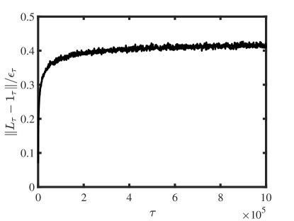
Figure 1: $\frac{\|L_{\tau}-\mathscr{L}_{\tau}\|}{\epsilon_{\tau}}$ against the regularizer $\tau$.

Set $\epsilon_{\tau}=(1+\sqrt{\frac{MN}{\tau+\delta_{\mathrm{min}}}})\sqrt{\frac{\rho\mathrm{max}(N,J)\mathrm{log}(N+J)}{\tau+\delta_{\mathrm{min}}}}$, which can be seen as a function of the regularization parameter $\tau$. It is easy to see that when all model parameters are fixed, $\epsilon_{\tau}$ decreases to zero as $\tau$ increases to infinity. In fact, $\|L_{\tau}-\mathscr{L}_{\tau}\|$ under LCM is usually smaller than $\epsilon_{\tau}$. To explain this statement, we provide a toy example in Figure 1 by plotting $\frac{\|L_{\tau}-\mathscr{L}_{\tau}\|}{\epsilon_{\tau}}$ against the regularizer $\tau$. For this figure, we let $N=500,J=200,K=3,M=5,\rho=1$, all entries of $\Theta$ be random values from a Uniform distribution on $(0,1)$, and each subject belong to one of the three latent classes with equality probability. After setting $Z$ and $\Theta$, we can generate $R$ from LCM. Then we can plot $\frac{\|L_{\tau}-\mathscr{L}_{\tau}\|}{\epsilon_{\tau}}$ against $\tau$. From Figure 1, we observe that $\frac{\|L_{\tau}-\mathscr{L}_{\tau}\|}{\epsilon_{\tau}}$ is always smaller than 0.5, which confirms our statement. We also observe that $\frac{\|L_{\tau}-\mathscr{L}_{\tau}\|}{\epsilon_{\tau}}$ increases as $\tau$ increases, which means that $\epsilon_{\tau}$ represents a good order of $\|L_{\tau}-\mathscr{L}_{\tau}\|$.

Define $\hat{\mathcal{C}}=\hat{\mathcal{C}}_{1}\bigcup\hat{\mathcal{C}}_{2}\ldots\bigcup\hat{\mathcal{C}}_{K}$ as the set collecting all estimated partitions, where $\hat{\mathcal{C}}_{k}=\{i:\hat{Z}(i,k)=1\mathrm{~{}for~{}}i\in[N]\}$ for $k\in[K]$. To evaluate the difference between the ground-truth classification set $\mathcal{C}$ and the estimated classification set $\hat{\mathcal{C}}$, we consider the Clustering error used in [17]. This measure is defined as

$$\hat{f}=\mathrm{min}_{\pi\in S_{K}}\mathrm{max}_{k\in[K]}\frac{|\mathcal{C}_{k}\cap\mathcal{\hat{\mathcal{C}}}^{c}_{\pi(k)}|+|\mathcal{C}^{c}_{k}\cap\mathcal{\hat{\mathcal{C}}}_{\pi(k)}|}{N_{K}},$$ (6)

where $S_{K}$ means all permutations of $\{1,2,\ldots,K\}$ and the superscript $c$ means the complementary sets. According to the reference [17], we know that the Clustering error $\hat{f}$ quantifies the maximum proportion of subjects in the symmetric difference of $\mathcal{C}_{k}$ and $\hat{\mathcal{C}}_{\pi(k)}$.

Our main result, which bounds the Clustering errors of LCA-RSC and LCA-RSCn, is presented below.

Theorem 1.

Under $\mathrm{LCM}(Z,\Theta)$, when Assumption 1 is satisfied, with probability at least $1-o((N+J)^{-3})$,

$$\hat{f}=O((1+\frac{MN}{\tau+\delta_{\mathrm{min}}}+2\sqrt{\frac{MN}{\tau+\delta_{\mathrm{min}}}})\frac{K^{2}(\tau+\delta_{\mathrm{max}})N_{\mathrm{max}}\mathrm{max}(N,J)\mathrm{log}(N+J)}{(\tau+\delta_{\mathrm{min}})\rho\sigma^{2}_{K}(B)N^{2}_{\mathrm{min}}})\mathrm{~{}and~{}}\frac{\|\hat{\Theta}-\Theta\|_{F}}{\|\Theta\|_{F}}=O(\sqrt{\frac{K~{}\mathrm{max}(N,J)\mathrm{log}(N+J)}{\rho N_{\mathrm{min}}\sigma^{2}_{K}(B)}}),$$

where $\delta_{\mathrm{max}}=\mathrm{max}_{i\in[N]}\mathscr{D}(i,i)$ and $\sigma_{K}(B)$ denotes $B$’s $K$-th largest singular value.

Note that LCA-RSC and LCA-RSCn have the same theoretical error rates. Theorem 1 says that the error rates are smaller when we increase the sparsity parameter $\rho$. We also find that if the minimize size of a latent class (and $\sigma_{K}(B)$) is too small, then the error rates are large, i.e., a harder scenario for latent class analysis. Sure, Theorem 1 also works for the binary response data case by simply setting $M=1$.

Choice of $\tau$ : Theoretical bounds in Theorem 1 depends on the regularization parameter $\tau$ through the term $\varrho_{\tau}=(1+\frac{MN}{\tau+\delta_{\mathrm{min}}}+2\sqrt{\frac{MN}{\tau+\delta_{\mathrm{min}}}})\frac{\tau+\delta_{\mathrm{max}}}{\tau+\delta_{\mathrm{min}}}$. Because $0<\delta_{\mathrm{min}}\leq\delta_{\mathrm{max}}=\mathrm{max}_{i\in[N]}\sum_{j=1}^{J}\mathscr{R}(i,j)\leq\rho J\leq M\mathrm{max}(N,J)$, Theorem 1 implies that increasing $\tau$ decreases the upper bounds of error rates. Suppose that $\tau\geq M\mathrm{max}(N,J)$, we have $\frac{MN}{\tau+\delta_{\mathrm{min}}}\leq 1,\frac{\tau+\delta_{\mathrm{max}}}{\tau+\delta_{\mathrm{min}}}=O(1)$, and $\varrho_{\tau}=O(1)$, which suggests that the results in Theorem 1 can be simplified as $\hat{f}=O(\frac{K^{2}N_{\mathrm{max}}\mathrm{max}(N,J)\mathrm{log}(N+J)}{\rho\sigma^{2}_{K}(B)N^{2}_{\mathrm{min}}})$. On the one hand, we cannot let $\tau$ too large because $\|L_{\tau}\|=\|D^{-1/2}_{\tau}R\|\leq\|D^{-1/2}_{\tau}\|\|R\|=\frac{\|R\|}{\sqrt{\tau+\mathrm{min}_{i\in[N]}D(i,i)}}$, which suggests that $L_{\tau}$’s top-$K$ singular values are close to zero for a too large $\tau$ and this causes that $L_{\tau}$’s top-$K$ singular vectors may lose valuable information about latent classes. On the other hand, by analyzing the form of $\varrho_{\tau}$, we find that though a larger $\tau$ is always preferred either for the case $\delta_{\mathrm{min}}\ll\delta_{\mathrm{max}}$ or the case $\delta_{\mathrm{min}}=O(\delta_{\mathrm{max}})$, continuing to increase the value of $\tau$ will not significantly reduce $\varrho_{\tau}$ since $\varrho_{\tau}$ is always at the order $O(1)$ when $\tau\geq M\mathrm{max}(N,J)$, i.e., $\varrho_{\tau}$ is insensitive for large $\tau$. Therefore, a moderate value of the regularizer $\tau$ is preferred. In numerical studies, we find that setting $\tau=M\mathrm{max}(N,J)$ provides satisfactory results.

From now on, unless specified, we set $\tau=M\mathrm{max}(N,J)$. If we consider more conditions on model parameters, Theorem 1 can be further simplified using the following corollary.

Corollary 1.

Under $\mathrm{LCM}(Z,\Theta)$, suppose that Assumption 1 holds. If $K=O(1),N_{\mathrm{min}}=O(\frac{N}{K}),N_{\mathrm{max}}=O(\frac{N}{K}),J=O(N)$, and $\sigma^{2}_{K}(B)=O(J)$, then with probability at least $1-o((N+J)^{-3})$,

$$\hat{f}=O(\frac{\mathrm{log}(N)}{\rho N})\mathrm{~{}and~{}}\frac{\|\hat{\Theta}-\Theta\|_{F}}{\|\Theta\|_{F}}=O(\sqrt{\frac{\mathrm{log}(N)}{\rho N}}).$$

In Corollary 1, all conditions are mild: $K=O(1)$ means that the number of latent classes is a small positive integer, $N_{\mathrm{min}}=O(\frac{N}{K})$ and $N_{\mathrm{max}}=O(\frac{N}{K})$ means that the sizes of each latent class are in the same order, $J=O(N)$ means that $J$ is in the same order as $N$, and $\sigma^{2}_{K}(B)=O(J)$ is also mild since $B$ is a $J$-by-$K$ matrix and $B$’s maximum entry is 1. By Corollary 1, it is clear to see that the error rates tend to zero as the number of subjects $N$ goes to infinity. Thus, LCA-RSC and LCA-RSCn are consistent in latent class analysis.

5 Quantifying the quality of latent class analysis

Our algorithms will normally be applied to study the latent classes for real-world categorical data for which the ground-truth latent classes are usually unknown in advance. Recall that our algorithms can always return some partitions of all subjects into different classes, this naturally leads to the following problem: is there a way to tell us whether the estimated latent classes returned by our algorithms are good or not? Meanwhile, when there are many different algorithms in latent class analysis, we also want to compare their performances and choose the one that returns the best partition. Furthermore, the number of latent classes, $K$, is usually unknown for real data, which raises the following problem: can we design an efficient approach to estimate $K$?

To answer these problems, we now focus on the binary data case to simplify our analysis. For this case, $R(i,j)\in\{0,1\}$ for $i\in[N],j\in[J]$. Define $A$ as $A=RR^{\prime}$ and call it the adjacency matrix in this article. From the definition of the adjacency matrix $A$, we have the following two facts:

• $A(i,i)=\sum_{j=1}^{J}R(i,j)$, i.e., the summation of responses of subject $i$ to all items for $i\in[N]$.

• For $i\neq\bar{i}$, $A(i,\bar{i})=\sum_{j=1}^{J}R(i,j)R(\bar{i},j)$, i.e., the number of common responses between the two subjects $i,\bar{i}$.

Suppose that there are three subjects $i,\bar{i},$ and $\tilde{i}$ such that subject $i$ and subject $\bar{i}$ are in the same latent class while subject $\tilde{i}$ is from a different latent class. Because subjects in the same latent class usually have similar response patterns, generally, subjects $i$ and $\bar{i}$ have more common responses than that of subjects $i$ and $\tilde{i}$. For the categorical data case, we can also define the adjacency matrix $A$ as $RR^{\prime}$, and a further understanding of $A$ is similar to that of the binary data case. Therefore, such adjacency matrix $A$ naturally forms an assortative weighted network [28] in which nodes within the same class connect more than nodes across classes. Based on this observation, it is natural to use the Newman-Girvan modularity [30, 29] to measure the quality of class partition for latent class analysis using the matrix $A$. Let $d_{i}=\sum_{j=1}^{N}A(i,j)$ for $i\in[N]$. Let $\omega=\frac{1}{2}\sum_{i=1}^{N}d_{i}$. Suppose that $\hat{Z}$ is an $N$-by-$k$ matrix obtained by applying a latent class analysis algorithm $\mathcal{M}$ on the observed response matrix $R$ with $k$ latent classes. The Newman-Girvan modularity is calculated as

$$Q_{\mathcal{M}}(k)=\frac{1}{2\omega}\sum_{i=1}^{N}\sum_{j=1}^{N}(A(i,j)-\frac{d_{i}d_{j}}{2\omega})\hat{Z}(i,:)\hat{Z}^{\prime}(j,:).$$ (7)

We always prefer a larger value of modularity since it usually indicates a better quality of latent class partitions [29]. After defining the modularity, to infer the number of latent classes $K$, the idea introduced in [27] is adopted. In detail, we choose the $k$ that maximizes the modularity defined in Equation (7), i.e.,

$$\hat{K}_{\mathcal{M}}=\mathrm{arg~{}max}_{k\in[\mathrm{min}(N,J)]}Q_{\mathcal{M}}(k).$$ (8)

It should be noted that the estimated classification matrix $\hat{Z}$ in Equation (7) is returned by an arbitrary algorithm $\mathcal{M}$, thus the estimated number of latent classes in Equation (8) can be different for different algorithms. For convenience, when algorithm $\mathcal{M}$ is applied to Equation (8), we call our approach for estimating $K$ as K$\mathcal{M}$.

6 Experimental results

In this section, both numerical and empirical studies are conducted. Meanwhile, all experimental studies in this article are reported using MATLAB R2021b. Before starting our experimental studies, we provide several baseline methods and some criteria for measuring the performance of different approaches.

6.1 Baseline methods

Here, we provide four alternative spectral clustering algorithms that can also fit the latent class model.

6.1.1 LCA-RSCORS

We call the first alternative method LCA-RSCORS, where RSCORS is short for regularized spectral clustering on ratios-of-singular-vectors. Let $U=[\eta_{1},\eta_{2},\ldots,\eta_{K}]$, where $\eta_{k}$ is the left singular vector of the $k$-th largest singular value of $\mathscr{L}_{\tau}$. Define the $N\times(K-1)$ matrix $\Xi$ such that $\Xi(i,k)=\frac{\eta_{k+1}(i)}{\eta_{1}(i)}$ for $i\in[N],k\in[K-1]$. According to the proof of Lemma 1, we get $U=\mathscr{D}^{-1/2}_{\tau}Z\Theta^{\prime}V\Sigma^{-1}$, which gives that $\Xi=Z\Xi(\mathcal{I},:)$, i..e, $\Xi$ has $K$ distinct rows and $\Xi(i,:)=\Xi(\bar{i},:)$ if $\ell(i)=\ell(\bar{i})$. Thus running the K-means approach to all rows of $\Xi$ exactly recovers $Z$. The above analysis suggests the following algorithm called Ideal LCA-RSCORS. Input: $\mathscr{R},K$, and $\tau$. Output: $Z$ and $\Theta$.

• Calculate $\mathscr{L}_{\tau}$ by Equation (3).

• Obtain $U\Sigma V^{\prime}$, the top $K$ SVD of $\mathscr{L}_{\tau}$. Then calculate the $N\times(K-1)$ matrix $\Xi$ from $U.$

• Run K-means algorithm on all rows of $\Xi$ with $K$ clusters to obtain $Z$.

• Recover $\Theta$ by setting $\Theta=\mathscr{R}^{\prime}Z(Z^{\prime}Z)^{-1}$.

For the real case with only known the observed response matrix $R$, let $\hat{U}=[\hat{\eta}_{1},\hat{\eta}_{2},\ldots,\hat{\eta}_{K}]$, where $\hat{\eta}_{k}$ is the left singular vector of the $k$-th largest singular value of the regularized Laplacian matrix $L_{\tau}$ for $k\in[K]$. Let $\hat{\Xi}$ be an $N\times(K-1)$ matrix such that $\hat{\Xi}(i,k)=\frac{\hat{\eta}_{k+1}(i)}{\hat{\eta}_{1}(i)}$ for $i\in[N],k\in[K]$. The following algorithm extends the Ideal LCA-RSCORS to the real case.

Algorithm 5 LCA-RSCORS

1:$R,K$, and $\tau$ (the default $\tau$ is $M\mathrm{max}(N,J)$.).

2:$\hat{Z}$ and $\hat{\Theta}$.

3:Calculate the regularize Laplacian matrix $L_{\tau}$ by Equation (5).

4:Obtain $\hat{U}\hat{\Sigma}\hat{V}^{\prime}$, the top $K$ SVD of $L_{\tau}$. Then calculate the $N\times(K-1)$ matrix $\hat{\Xi}$ from $\hat{U}$.

5:Run K-means algorithm on all rows of $\hat{\Xi}$ with $K$ clusters to obtain $\hat{Z}$.

6:Obtain $\hat{\Theta}$ using Steps 4-5 of Algorithm 3.

LCA-RSCORS has the same computational complexity as LCA-RSC and LCA-RSCn. Due to the row-wise ratios matrices $\Xi$ and $\hat{\Xi}$, it is complex to obtain the theoretical bounds of LCA-RSCORS. One possible way to obtain LCA-RSCORS’s theoretical guarantees is to combine the theoretical analysis in this article with the proofs of the community detection algorithms provided in [15, 43]. The theoretical framework of LCA-RSCORS is of independent interest.

6.1.2 LCA-PCA

We name the second alternative method as LCA-PCA, where PCA is short for principle component analysis. Recall that the rank of the $N\times J$ population response matrix $\mathscr{R}$ is also $K$. Without confusion, we let $\mathscr{R}=U\Sigma V^{\prime}$ be the top-K SVD of $\mathscr{R}$ such that $U^{\prime}U=I_{K\times K}$ and $V^{\prime}V=I_{K\times K}$. Following a similar analysis to the 2nd statement of Lemma 1 gives $U=ZU(\mathcal{I},:)$, which implies that running the K-means procedure to $U$’s rows returns the classification matrix $Z$. This suggests the following method called Ideal LCA-PCA. Input: $\mathscr{R}$ and $K$. Output: $Z$ and $\Theta$.

• Obtain $U\Sigma V^{\prime}$, the top $K$ SVD of $\mathscr{R}$.

• Run K-means algorithm on $U$’s rows with $K$ clusters to obtain $Z$.

• Recover $\Theta$ by setting $\Theta=\mathscr{R}^{\prime}Z(Z^{\prime}Z)^{-1}$.

Let $\hat{U}\hat{\Sigma}\hat{V}^{\prime}$ be $R$’s top-K SVD. Algorithm 6 extends Ideal LCA-PCA to the real case immediately.

Algorithm 6 LCA-PCA

1:$R$ and $K$.

2:$\hat{Z}$ and $\hat{\Theta}$.

3:Obtain $\hat{U}\hat{\Sigma}\hat{V}^{\prime}$, the top $K$ SVD of $R$.

4:Run K-means algorithm on $\hat{U}$’s rows with $K$ clusters to obtain $\hat{Z}$.

5:Obtain $\hat{\Theta}$ using Steps 4-5 of Algorithm 3.

Compared with LCA-RSC, LCA-RSCn, and LCA-RSCORS, we design LCA-PCA using the SVD of the observed response matrix instead of the regularized Laplacian matrix. Meanwhile, LCA-PCA has the same computational complexity as LCA-RSC, LCA-RSCn, and LCA-RSCORS. Following a similar analysis as Theorem 1 gets LCA-PCA’s theoretical error rates, which are almost the same as that of LCA-RSC and we omit them here.

6.1.3 LCA-RMK

Because $\mathscr{R}=Z\Theta^{\prime}$ under $\mathrm{LCM}(Z,\Theta)$, we have $\mathscr{R}=Z\mathscr{R}(\mathcal{I},:)$. Thus applying the K-means algorithm on $\mathscr{R}$’s rows with $K$ clusters returns $Z$. This gives the following algorithm called Ideal LCA-RMK, where RMK is short for response matrix by K-means. Input: $\mathscr{R}$ and $K$. Output: $Z$ and $\Theta$.

• Run K-means algorithm on $\mathscr{R}$’s rows with $K$ clusters to obtain $Z$.

• Recover $\Theta$ by setting $\Theta=\mathscr{R}^{\prime}Z(Z^{\prime}Z)^{-1}$.

Algorithm 7 LCA-RMK

1:$R$ and $K$.

2:$\hat{Z}$ and $\hat{\Theta}$.

3:Run K-means algorithm on $R$’s rows with $K$ clusters to obtain $\hat{Z}$.

4:Obtain $\hat{\Theta}$ using Steps 4-5 of Algorithm 3.

Algorithm 7 called LCA-RMK extends the Ideal LCA-RMK to the real case naturally. Unlike LCA-RSC, LCA-RSCn, LCA-RSCORS, and LCA-PCA, there is no SVD step in LCA-RMK. The computational cost of LCA-RMK is $O(lNJK)$ with $l$ being the number of iterations in K-means. For the case $J=\beta N$, LCA-RMK’s complexity is $O(\beta lKN^{2})$, which is slightly larger than $O(KN^{2})$ when $\beta l>1$. Therefore, LCA-RSC, LCA-RSCn, LCA-RSCORS, and LCA-PCA run faster than LCA-RMK when $\beta l>1$. This conclusion is verified by the experimental results in this section.

6.1.4 LCA-RLMK

Similar to the Ideal-RMK, recall that $\mathscr{L}_{\tau}=\mathscr{D}^{-1/2}_{\tau}Z\Theta^{\prime}$, we also have $\mathscr{L}_{\tau}=Z\mathscr{L}_{\tau}(\mathcal{I},:)$ by simple algebra, which suggests the following algorithm called Ideal LCA-RLMK, where RLMK is short for regularized Laplacian matrix by K-means. Input: $\mathscr{R},K$, and $\tau$. Output: $Z$ and $\Theta$.

• Calculate $\mathscr{L}_{\tau}$ by Equation (3).

• Run K-means algorithm on $\mathscr{L}_{\tau}$’s rows with $K$ clusters to obtain $Z$.

• Recover $\Theta$ by setting $\Theta=\mathscr{R}^{\prime}Z(Z^{\prime}Z)^{-1}$.

Algorithm 8 LCA-RLMK

1:$R,K$, and $\tau$ with default value $M\mathrm{max}(N,J)$.

2:$\hat{Z}$ and $\hat{\Theta}$.

3:Calculate $L_{\tau}$ by Equation (5).

4:Run K-means algorithm on $L_{\tau}$’s rows with $K$ clusters to obtain $\hat{Z}$.

5:Obtain $\hat{\Theta}$ using Steps 4-5 of Algorithm 3.

Algorithm 8 summarizes the real case of Ideal LCA-RLMK. This algorithm has the same computational complexity as LCA-RMK.

6.2 Evaluation metrics

For the task of classification when the true classification matrix $\mathbf{Z}$ is known, four metrics are considered: Clustering error $\hat{f}$ computed by Equation (6), Hamming error [15], normalized mutual information (NMI) [38, 8, 3, 23], and adjusted rand index (ARI) [23, 14, 41]. Hamming error is defined as $\frac{\mathrm{min}_{\mathcal{P}\in\mathcal{P}_{K}}|i:\hat{Z}(i,:)\neq(Z\mathcal{P})(i,:)\mathrm{~{}for~{}}i\in[N]|}{N}$, where $\mathcal{P}_{K}$ is the set containing all $K\times K$ permutation matrices. Hamming error ranges in $[0,1]$, and a smaller Hamming error means a better estimation. The exact forms of NMI and ARI can be found in Equations (5) and (6) in [34]. NMI ranges in [0,1], ARI ranges in [-1,1], and both metrics are the larger the better.

For the task of classification when the true classification matrix $\mathbf{Z}$ is unknown, we use the Newman-Girvan modularity calculated by Equation (7) using the adjacency matrix $A=RR^{\prime}$ to measure the quality of latent class analysis.

For the task of estimating $\mathbf{\Theta}$, we use the Relative $l_{1}$ error defined as $\mathrm{min}_{\mathcal{P}\in\mathcal{P}_{K}}\frac{\|\hat{\Theta}-\Theta\mathcal{P}\|_{1}}{\|\Theta\|_{1}}$ and the Relative $l_{2}$ error defined as $\mathrm{min}_{\mathcal{P}\in\mathcal{P}_{K}}\frac{\|\hat{\Theta}-\Theta\mathcal{P}\|_{F}}{\|\Theta\|_{F}}$ to measure the performance, where $\|\cdot\|_{1}$ for a matrix means its $l_{1}$ norm. Both measures are the smaller the better.

For the task of estimating the number of latent classes $\mathbf{K}$, we use Accuracy rate to measure the performances of all K$\mathcal{M}$ methods. This metric is defined as the fraction of times a method correctly determines $K$. Recall that this article develops six algorithms LCA-RSC, LCA-RSCn, LCA-RSCORS, LCA-PCA, LCA-RMK, and LCA-RLMK for latent class analysis. As a result, there are six algorithms KLCA-RSC, KLCA-RSCn, KLCA-RSCORS, KLCA-PCA, KLCA-RMK, and KLCA-RLMK for determining $K$.

6.3 Synthetic categorical data

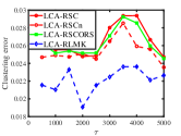
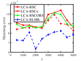
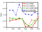
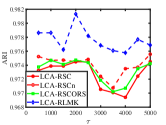
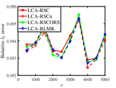
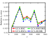
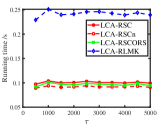
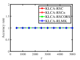
Figure 2: Numerical results of Experiment 1.

Our numerical studies focus on three issues: the choice of the regularizer $\tau$, the effectiveness of all aforementioned methods in latent class analysis, and the accuracy of our methods for estimating $K$. Unless specified, we set $K=3,J=\frac{N}{5}$, and $M=5$. Note that since we let $M$ be $5$ in our numerical studies, $R(i,j)$ takes value from the set $\{0,1,2,3,4,5\}$ for $i\in[N],j\in[J]$, which suggests a categorical data case. $Z$ is generated by letting each subject belong to one of the $K$ latent classes with equal probability. Let $\tilde{B}$ be a $J$-by-$K$ matrix such that $\tilde{B}(j,k)=\mathrm{rand}(1)$ for $i\in[J],k\in[K]$, where $\mathrm{rand}(1)$ is a random value generated from a Uniform distribution on $[0,1]$. Let $B=\frac{\tilde{B}}{\mathrm{max}_{j\in[J],k\in[K]}\tilde{B}(j,k)}$ (thus, $\mathrm{max}_{j\in[J],k\in[K]}B(j,k)=1$ is guaranteed). We set $\rho$ and $N$ independently for each experiment. Except for the experiment that studies the choice of $\tau$, we set $\tau$ as the default value $M\mathrm{max}(N,J)$. After setting $Z$ and $\Theta$, each numerical experiment has below steps:

(a)

For $i\in[N],j\in[J]$, generate $R(i,j)$ from a Binomial distribution with $M$ independent trials and probability $\frac{\mathscr{R}(i,j)}{M}$, where $\mathscr{R}=Z\Theta^{\prime}=\rho ZB^{\prime}$.

(b)

Apply our proposed methods to $R$. Record each metric and running time of all methods.

(c)

Repeat (a)-(b) 100 times and report the mean of each metric.

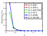
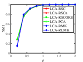
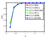
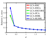
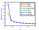
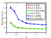
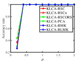
Figure 3: Numerical results of Experiment 2.

In this article, we conduct the following four Experiments.

Experiment 1: Choice of the regularizer $\tau$. Recall that the regularization parameter $\tau$ appears in our LCA-RSC, LCA-RSCn, LCA-RSCORS, and LCA-RLMK methods. Here, we study the choice of $\tau$ numerically. For this experiment, we set $\rho=0.8,N=500$, and $\tau=c_{0}M\mathrm{max}(N,J)$. We vary $c_{0}$ in the range $\{0.2,0.4,\ldots,2\}$. The results can be found in Figure 2. From panels (a)-(f) of Figure 2, we observe that the four methods have the smallest Clustering error, Hamming error, Relative $l_{1}$ error, and Relative $l_{2}$ error when $\tau$ is set around $M\mathrm{max}(N,J)$; they also have the largest NMI and ARI when $\tau$ is around $M\mathrm{max}(N,J)$. This suggests that setting $\tau$ as $M\mathrm{max}(N,J)$ is a good choice for these methods. Meanwhile, we also find that all metrics in panels (a)-(f) do not change significantly when $\tau$ increases and this verifies our analysis after Theorem 1 that the error rates are insensitive for large $\tau$. From Panel (g) of Figure 2, we see that LCA-RSC, LCA-RSCn, and LCA-RSCORS run faster than LCA-RLMK, which verifies our complexity analysis provided after Algorithm 7 and Algorithm 8. The last panel of Figure 2 says that KLCA-RSC, KLCA-RSCn, KLCA-RSCORS, and K-LCA-RLMK determines the number of classes $K$ correctly in this experiment, which also supports the effectiveness of our idea that using Newman-Girvan modularity to measure the quality of latent class when the adjacency matrix $A$ is set as $RR^{\prime}$.

Experiment 2: Changing the sparsity parameter $\rho$. For this experiment, we investigate the performances of our methods by changing $\rho$ when $N=500$. Because $\rho$ should be no larger than the number of trials $M$ under Binomial distribution, here we let $\rho$ take value in the set $\{0.2,0.4,\ldots,2\}$. Figure 3 presents the results. From the first six panels, we observe that all methods perform similarly and they perform better when the sparsity parameter increases, which confirms our theoretical analysis provided after Theorem 1. From panel (g) of Figure 3, we observe that LCA-RMK and LCA-RLMK run slower than the other four methods, which supports our analysis after Algorithm 7 and Algorithm 8. Meanwhile, we also see that all methods run faster as the sparsity parameter becomes bigger. Finally, the last panel tells us that our methods for estimating $K$ perform better as $\rho$ increases and they exactly infer $K$ when $\rho$ is no smaller than 0.5 for this experiment. Again, the high accuracy of our methods in estimating $K$ suggests the success of using the Newman-Girvan modularity to evaluate the quality of latent class analysis.

Experiment 3: Changing the number of subjects $N$. For this experiment, we study the performances of all approaches by increasing $N$ when $\rho=0.15$. We let $N$ range in $\{1000,2000,\ldots,8000\}$. Figure 4 shows the results. The first six panels say that all methods have similar performances in estimating $Z$ and $\Theta$, and they perform better as $N$ increases, which supports our analysis after Theorem 1. Panel (g) of Figure 4 says that LCA-RSC, LCA-RSCn, LCA-RSCORS, and LCA-PCA run faster than LCA-RMK and LCA-RLMK, which also verifies our analysis after Algorithm 7. Meanwhile, from panel (g), we also observe that LCA-RSC, LCA-RSCn, LCA-RSCORS, and LCA-PCA process a response matrix of up to 8000 subjects and 1600 items within five seconds, which suggests the effectiveness of our methods in latent class analysis. The last panel shows that our methods are accurate in deciding the number of latent classes, which implies the effectiveness of the Newman-Girvan modularity in turn.

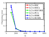
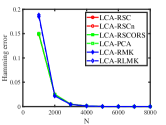
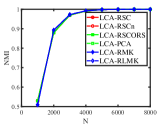
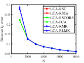
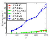
Figure 4: Numerical results of Experiment 3.

Experiment 4: A simple example. Here, we provide a toy example by generating only one response matrix. For this experiment, we set $K=2,M=3,N=16$, and $J=10$. In Figure 5, the 1st, 2nd, and 3rd matrices show $Z,\Theta$, and a response matrix $R$ generated from a Binomial distribution with expectation $Z\Theta^{\prime}$ and 3 independent trials. Applying our methods to the observed response matrix $R$ (i.e., the 3rd matrix in Figure 5) obtains their respective metrics, which are shown in Table 1. We see that all methods exactly recover $Z$ and exactly infer $K$ for this example. All methods also return the same $\hat{\Theta}$ which is the 4th matrix in Figure 5. Because $Z$ and $\Theta$ are provided in the first two matrices of Figure 5, readers can run our algorithms or some other algorithms to the $R$ in the 3rd matrix of Figure 5 to verify their accuracies in estimating $Z,\Theta$, and $K$.

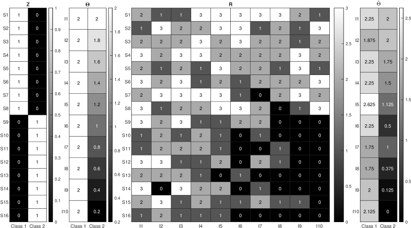
Figure 5: The 1st and 2nd matrices are $Z$ and $\Theta$ for Experiment 4, respectively. The 3rd matrix is an observed response matrix $R$ generated from LCM using $Z$ and $\Theta$ in the first two matrices when the number of independent trials $M=3$ in a Binomial distribution. The last matrix is the estimated item parameter matrix $\hat{\Theta}$ returned by all algorithms. For all matrices, S$i$ represents subject $i$ for $i\in[16]$ and I$j$ represents item $j$ for $j\in[10]$.

Table 1: Metrics and $\hat{K}$ of our methods for $R$ in the 3rd matrix of Figure 5, where $\hat{K}$ is the output of Equation (8) for each method.

	Clustering error	Hamming error	NMI	ARI	Relative $l_{1}$ error	Relative $l_{2}$ error	$\hat{K}$
LCA-RSC	0	0	1	1	0.1188	0.1550	2
LCA-RSCn	0	0	1	1	0.1188	0.1550	2
LCA-RSCORS	0	0	1	1	0.1188	0.1550	2
LCA-PCA	0	0	1	1	0.1188	0.1550	2
LCA-RMK	0	0	1	1	0.1188	0.1550	2
LCA-RLMK	0	0	1	1	0.1188	0.1550	2

6.4 Real data applications

For empirical studies, we apply algorithms developed in this article to real-world categorical data.

Table 2: Estimated number of latent classes and the respective modularity of all methods for real data considered in this paper. The 1st value in the bracket represents $\hat{K}_{\mathcal{M}}$ and the 2nd value in the bracket represents $Q_{\hat{K}_{\mathcal{M}}}$ for method $\mathcal{M}$.

Dataset	LCA-RSC	LCA-RSCn	LCA-RSCORS	LCA-PCA	LCA-RMK	LCA-RLMK
MovieLens 100k	(3, 0.0941)	(3, 0.0990)	(3, 0.0729)	(3, 0.0933)	(4, 0.0667)	(4, 0.0673)
IPIP	(2, 0.0077)	(2, 0.0077)	(2, 0.0073)	(2, 0.0077)	(2, 0.0071)	(2, 0.0071)

6.4.1 MovieLens 100k data

The MovieLens 100k [18] is a user-movie ratings data set that is available at the link http://konect.cc/networks/movielens-100k_rating/. This data consists of 943 users and 1682 movies. For this data, the rating scores range in $\{0,1,2,3,4,5\}$, where 0 means no rating, and the higher the user’s rating for a movie, the more he/she likes it. Therefore we have $R\in\{0,1,2,3,4,5\}^{943\times 1682}$. To choose how many latent classes should be used for the MovieLens 100k data, we apply our methods to its observed response matrix $R$ using Equation (7). The results reported in Table 2 suggest that $K=3$ is most appropriate for the MovieLens 100k data because LCA-RSCn returns the largest modularity value 0.0990 when $K=3$. For this reason, the LCA-RSCn method should be applied to the MovieLens 100k data with 3 latent classes. Applying LCA-RSCn to this data when $K=3$, we get the $943\times 3$ matrix $\hat{Z}$ and the $1682\times 3$ matrix $\hat{\Theta}$. For convenience, we denote the estimated latent classes as Class 1, Class 2, and Class 3. Based on $\hat{Z}$, we find that Class 1, 2, and 3 have 237, 253, and 453 users, respectively. For visualization, we plot the estimated latent classes for the top 30 users and the estimated item parameter matrix for the top 30 movies in Figure 6. We can find the estimated latent class for each class clearly from the 1st matrix in Figure 6. The strength of preference on each movie for users in the same latent class can be found from the 2nd matrix in Figure 6, where Remark 3 explains why $\hat{\Theta}(j,k)$ reflects the strength of preference for users in the $k$-th latent class to the $j$-th movie for $j\in[1682],k\in[3]$. For example, users in Class 1 tend to give higher rating scores than that of users in Classes 2 and 3 for Movies 1-5, 7, 11, 15, 17, 21, 22, 24, 25, 27, and 29; users in Class 2 give higher rating scores than that of users in Class 3 for Movies 1, 2, 4-23, 25-26, and 27-30. In fact, by analyzing the $1682\times 3$ matrix $\hat{\Theta}$, we find that $\sum_{j=1}^{1682}\hat{\Theta}(j,1)=604.9283,\sum_{j=1}^{1682}\hat{\Theta}(j,2)=502.6364$, and $\sum_{j=1}^{1682}\hat{\Theta}(j,3)=182.0110$, which suggests that users in Class 1 tend to give higher rating scores than users in Class 2 and Class 3 while users in Class 2 tend to give higher values than users in Class 3. Based on this finding, we interpret Class 1 as users who hold an optimistic view of movies, Class 2 as users who hold a neutral view of movies, and Class 3 as users who hold a passive view of movies.

Remark 3.

Let $\hat{N}_{k}=\sum_{i=1}^{N}\hat{Z}(i,k)$ for $k\in[K]$, i.e., $\hat{N}_{k}$ denotes the size of the $k$-th estimated latent class. By the 4th and 5th steps of Algorithm 3, we have $\hat{\Theta}(j,k)$ roughly equals to $\frac{\sum_{i:\hat{Z}(i,k)==1\mathrm{~{}for~{}}i\in[N]}R(i,j)}{\hat{N}_{k}}$ for $j\in[J],k\in[K]$. Therefore, similar to $\Theta(j,k)$, $\hat{\Theta}(j,k)$ also denotes the averaged response for subjects in the $k$-th estimated latent class to the $j$-th item.

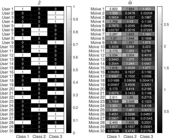
Figure 6: Left matrix: Heatmap of $\hat{Z}$ of a subset of 30 users for the MovieLens 100k data. Right matrix: Heatmap of $\hat{\Theta}$ of a subset of 30 movies for the MovieLens 100k data.

6.5 International Personality Item Pool (IPIP) personality test data

Our methods are also applied to deal with a psychological test dataset, the International Personality Item Pool (IPIP) personality test data. It can be downloaded from https://openpsychometrics.org/_rawdata/ and it contains responses of 1005 individuals to 40 personality test questions. After removing one individual that does not respond to any test question, we get $N=1004$. For this data, 0, 1, 2, 3, 4, and 5 denote no response, strongly disagree, disagree, neither agree not disagree, agree, and strongly agree, respectively. Therefore, $R\in\{0,1,2,3,4,5\}^{1004\times 40}$. Questions 1-10, 11-20, 21-30, and 31-40 measure the personality factors Assertiveness (“AS”), Social confidence ( “SC”), Adventurousness (“AD”), and Dominance (“DO”), respectively. These questions can be found in the 2nd matrix of Figure 7. Table 2 reports the estimated number of latent classes and the respective modularity for each method. We see that all methods suggest $K=2$ for this data. Here, we also consider LCA-RSCn for the IPIP data because LCA-RSCn returns the largest value of modularity. Applying LCA-RSCn to IPIP with $K=2$, we get the $1004\times 2$ matrix $\hat{Z}$ and the $40\times 2$ matrix $\hat{\Theta}$. We also use Class 1 and Class 2 to denote the two estimated latent classes for the IPIP data. By analyzing $\hat{Z}$, we find that there are 475 individuals in Class 1 and 529 individuals in Class 2. For visualization, we plot the estimated latent classes for the top 40 individuals and $\hat{\Theta}$ in Figure 7. By carefully analyzing the heatmap of $\hat{\Theta}$, Class 1 can be interpreted as individuals who are socially passive/negative and Class 2 can be interpreted as individuals who are socially active/positive. Elements of $\hat{\Theta}$ imply that individuals in Class 2 are more expressional&active&ambitious&confident&creative&dominant&social&open than individuals in Class 1.

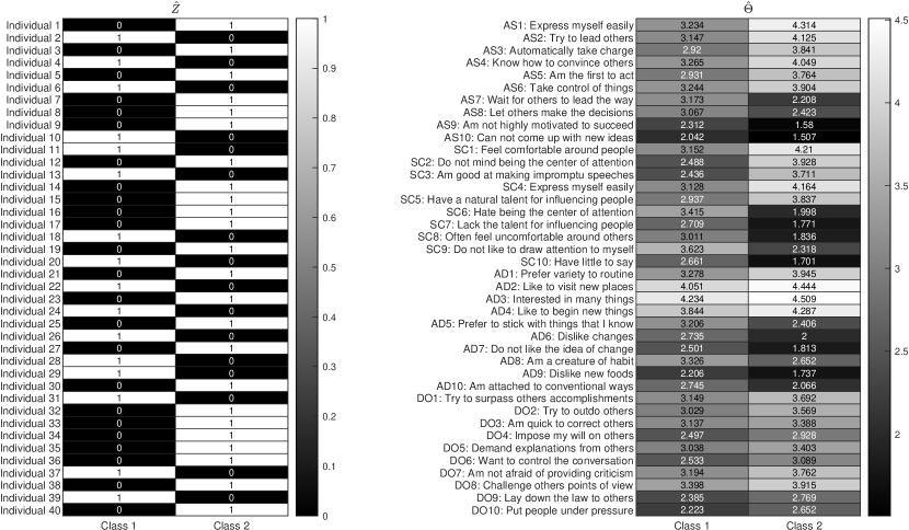
Figure 7: Left matrix: Heatmap of $\hat{Z}$ of a subset of 40 individuals for the IPIP data. Right matrix: Heatmap of $\hat{\Theta}$ for the IPIP data.

7 Conclusion

In this article, two efficient regularized spectral clustering algorithms are proposed for the latent class model in categorical data. This is the first time to design algorithms based on the newly defined regularized Laplacian matrix in latent class analysis for categorical data. We establish the theoretical guarantees for our algorithms by considering the sparsity parameter. We show that our algorithms can consistently recover the hidden classes and the item parameter matrix under a mild condition on the sparsity parameter. We also use a well-known modularity to evaluate the quality of latent class analysis. A strategy combining modularity with our algorithms is provided to determine how many latent classes are there for real-world categorical data. We conduct substantial experiments to demonstrate that our algorithms for latent class analysis are efficient and accurate, and our methods for estimating $K$ have satisfactory performances, which also supports the effectiveness of the modularity in quantifying the quality of latent class analysis in turn. We hope that our regularized spectral clustering algorithms, our idea of using modularity to measure the quality of latent class analysis, and our methods for estimating $K$ will have broad applications for categorical data in diverse fields like social, psychological, and behavioral sciences.

For future research, first, theoretical guarantees of LCA-RSCORS, LCA-RMK, and LCA-RLMK should be developed. Second, rigorous approaches should be proposed to determine $K$ under the latent class model for categorical data. Third, the grade of membership (GoM) model [45, 9] allows a subject to have partial memberships in different classes and it is more general than LCM. Thus, following ideas proposed in this article, designing regularized spectral clustering algorithms to estimate a grade of membership model is meaningful. Fourth, developing more efficient algorithms for latent class analysis to handle large-scale categorical data is an appealing topic.

CRediT authorship contribution statement

Huan Qing is the sole author of this article.

Declaration of competing interest

The author declares no competing interests.

Data availability

Data and code will be made available on request.

Appendix A Proofs under LCM

A.1 Proof of Lemma 1

Proof.

For the 1st statement, $\mathscr{R}=Z\Theta^{\prime}$ gives $\Theta Z^{\prime}=\mathscr{R}^{\prime}\Rightarrow\Theta Z^{\prime}Z=\mathscr{R}^{\prime}Z\Rightarrow\Theta=\mathscr{R}^{\prime}Z(Z^{\prime}Z)^{-1}$, where $Z^{\prime}Z$ is a $K\times K$ nonsingular matrix since $Z$’s rank is $K$.

For the 2nd statement, since $\mathscr{D}_{\tau}(i,i)=\tau+\sum_{j=1}^{J}\mathscr{R}(i,j)$ and $\mathscr{R}(i,j)=Z(i,:)\Theta^{\prime}(j,:)=\Theta(j,\ell(i))$, we get $\mathscr{D}_{\tau}(i,i)=\mathscr{D}_{\tau}(\bar{i},\bar{i})$ if $\ell(i)=\ell(\bar{i})$. Thus, the diagonal entries of $\mathscr{D}_{\tau}$ only have $K$ distinct values since all subjects belong to the $K$ latent classes.

Since $\mathscr{L}_{\tau}=\mathscr{D}^{-1/2}_{\tau}\mathscr{R}=\mathscr{D}^{-1/2}_{\tau}Z\Theta^{\prime}=U\Sigma V^{\prime}$, we have $U=\mathscr{D}^{-1/2}_{\tau}Z\Theta^{\prime}V\Sigma^{-1}$, which gives that $U(i,:)=\mathscr{D}^{-1/2}_{\tau}(i,i)Z(i,:)\Theta^{\prime}V\Sigma^{-1}$. Thus, we have $U(i,:)=U(\bar{i},:)$ if $\ell(i)=\ell(\bar{i})$ and $U$ has $K$ distinct rows since all subjects belong to the $K$ latent classes. Meanwhile, since $\mathscr{D}_{\tau}(i,i)=\mathscr{D}_{\tau}(\bar{i},\bar{i})$ when $\ell(i)=\ell(\bar{i})$, we have $U=\mathscr{D}^{-1/2}_{\tau}Z\Theta^{\prime}V\Sigma^{-1}=Z\mathscr{D}^{-1/2}_{\tau}(\mathcal{I},\mathcal{I})\Theta V^{\prime}\Sigma^{-1}$, i.e., $U=ZX$ with $X$ being $\mathscr{D}^{-1/2}_{\tau}(\mathcal{I},\mathcal{I})\Theta V^{\prime}\Sigma^{-1}\equiv U(\mathcal{I},:)$.

For the 3rd statement, we have $U_{*}(i,:)=\frac{U(i,:)}{\|U(i,:)\|_{F}}=\frac{Z(i,:)X}{\|Z(i,:)X\|_{F}}=\frac{X(\ell(i),:)}{\|X(\ell(i),:)\|_{F}}=U_{*}(\bar{i},:)$ if $\ell(i)=\ell(\bar{i})$, which gives that $U_{*}$ has $K$ distinct rows and $U_{*}=ZY$ with $Y$ being $U_{*}(\mathcal{I},:)$.

For the 4th statement, since $U^{\prime}U=I_{K\times K}$ and $U=ZX$, we have $X^{\prime}Z^{\prime}ZX=I_{K\times K}$, which gives that $XX^{\prime}=(Z^{\prime}Z)^{-1}=\mathrm{diag}(\frac{1}{N_{1}},\frac{1}{N_{2}},\ldots,\frac{1}{N_{K}})$. Then we get $X(k,:)X^{\prime}(k,:)=\frac{1}{N_{k}}$ and $X(k,:)X^{\prime}(l,:)=0$ for $k\neq l\in[K]$, which gives that $\|X(k,:)-X(l,:)\|_{F}=\sqrt{(X(k,:)-X(l,:))(X(k,:)-X(l,:))^{\prime}}=\sqrt{\frac{1}{N_{k}}+\frac{1}{N_{l}}}$ when $k\neq l$.

Since $Y=U_{*}(\mathcal{I},:)$ and $X=U(\mathcal{I},:)$, we have $Y(k,:)=\frac{X(k,:)}{\|X(k,:)\|_{F}}=\frac{X(k,:)}{\sqrt{X(k,:)X^{\prime}(k,:)}}=\sqrt{N_{k}}X(k,:)$ for $k\in[K]$. Thus, we have $Y(k,:)Y^{\prime}(l,:)=\sqrt{N_{k}N_{l}}X(k,:)X^{\prime}(l,:)=0$ when $k\neq l$ and $Y(k,:)Y^{\prime}(k,:)=N_{k}X(k,:)X^{\prime}(k,:)=1$ for $k\in[K]$. Finally, we have $\|Y(k,:)-Y(l,:)\|_{F}=\sqrt{(Y(k,:)-Y(l,:))(Y(k,:)-Y(l,:))^{\prime}}=\sqrt{2}$ when $k\neq l$. This completes the proof. ∎

A.2 Proof of Lemma 2

Proof.

First, the following result holds.

$$\|L_{\tau}-\mathscr{L}_{\tau}\| =\|D_{\tau}^{-1/2}R-\mathscr{D}^{-1/2}_{\tau}\mathscr{R}\|=\|D_{\tau}^{-1/2}R-\mathscr{D}^{-1/2}_{\tau}R+\mathscr{D}^{-1/2}_{\tau}R-\mathscr{D}^{-1/2}_{\tau}\mathscr{R}\|\leq\|\mathscr{D}^{-1/2}_{\tau}R-\mathscr{D}^{-1/2}_{\tau}\mathscr{R}\|+\|D_{\tau}^{-1/2}R-\mathscr{D}^{-1/2}_{\tau}R\|.$$

Next, we bound the two terms $\|\mathscr{D}^{-1/2}_{\tau}R-\mathscr{D}^{-1/2}_{\tau}\mathscr{R}\|$ and $\|D_{\tau}^{-1/2}R-\mathscr{D}^{-1/2}_{\tau}R\|$ separately.

We bound the first term using Theorem 1.6 in [39]. We describe this theorem below

Theorem 2.

(Theorem 1.6 of [39]) Let $\{X_{n}\}$ be a finite sequence that are independent, random matrices with dimensions $N\times J$. Assumes that

$$\mathbb{E}(X_{n})=0,\mathrm{and~{}}\|X_{n}\|\leq r~{}\mathrm{almost~{}surely}.$$

Then, for any $t\in[0,+\infty)$,

$$\mathbb{P}(\|\sum_{n}X_{n}\|\geq t)\leq(N+J)\cdot\mathrm{exp}(\frac{-t^{2}/2}{\sigma^{2}+rt/3}),$$

where $\sigma^{2}:=\mathrm{max}\{\|\sum_{n}\mathbb{E}(X_{n}X^{\prime}_{n})\|,\|\sum_{n}\mathbb{E}(X^{\prime}_{n}X_{n})\|\}$.

Set $e_{i}$ as an $N$-by-$1$ vector with $e_{i}(i)=1$ and $0$ elsewhere for $i\in[N]$, and $\tilde{e}_{j}$ as a $J$-by-$1$ vector with $\tilde{e}_{j}(j)=1$ and $0$ elsewhere for $j\in[J]$. Let $W=\mathscr{D}^{-1/2}_{\tau}R-\mathscr{D}^{-1/2}_{\tau}\mathscr{R}$. Then we can rewrite $W$ as $W=\sum_{i\in[N]}\sum_{j\in[J]}W(i,j)e_{i}\tilde{e}^{\prime}_{j}=\sum_{i\in[N]}\sum_{j\in[J]}W^{(i,j)}$, where $W^{(i,j)}=W(i,j)e_{i}\tilde{e}^{\prime}_{j}$. Under $\mathrm{LCM}(Z,\Theta)$, for $i\in[N],j\in[J]$, $\mathbb{E}(W(i,j))=0$ holds and

$$\|W^{(i,j)}\| =\frac{1}{\sqrt{\tau+\mathscr{D}(i,i)}}\|(R(i,j)-\mathscr{R}(i,j))e_{i}\tilde{e}^{\prime}_{j}\|\leq\frac{1}{\sqrt{\tau+\delta_{\mathrm{min}}}}|R(i,j)-\mathscr{R}(i,j)|\|e_{i}\tilde{e}^{\prime}_{j}\|\leq\frac{M}{\sqrt{\tau+\delta_{\mathrm{min}}}},$$

where the last inequality holds since $R(i,j)\in\{0,1,2,\ldots,M\},0\leq\mathscr{R}(i,j)\leq\rho\leq M$, and $\|e_{i}\tilde{e}^{\prime}_{j}\|=1$. Thus we have $r=\frac{M}{\sqrt{\tau+\delta_{\mathrm{min}}}}$.

Then we aim at bounding the variance term $\sigma^{2}=\mathrm{max}\{\|\sum_{i\in[N]}\sum_{j\in[J]}\mathbb{E}(W^{(i,j)}(W^{(i,j)})^{\prime})\|,\|\sum_{i\in[N]}\sum_{j\in[J]}\mathbb{E}((W^{(i,j)})^{\prime}W^{(i,j)})\|\}$. Because $R(i,j)\sim\mathrm{Binomial}(M,\frac{\mathscr{R}(i,j)}{M})$, we have $\mathbb{E}(W^{2}(i,j))=\frac{1}{\tau+\mathscr{D}(i,i)}\mathbb{E}((R(i,j)-\mathscr{R}(i,j))^{2})\leq\frac{1}{\tau+\delta_{\mathrm{min}}}\mathrm{Var}(R(i,j))=\frac{1}{\tau+\delta_{\mathrm{min}}}M\frac{\mathscr{R}(i,j)}{M}(1-\frac{\mathscr{R}(i,j)}{M})=\frac{1}{\tau+\delta_{\mathrm{min}}}\mathscr{R}(i,j)(1-\frac{\mathscr{R}(i,j)}{M})\leq\frac{1}{\tau+\delta_{\mathrm{min}}}\mathscr{R}(i,j)\leq\frac{\rho}{\tau+\delta_{\mathrm{min}}}$, which gives

$$\|\sum_{i=1}^{N}\sum_{j=1}^{J}\mathbb{E}(W^{(i,j)}(W^{(i,j)})^{\prime})\|=\|\sum_{i=1}^{N}\sum_{j=1}^{J}\mathbb{E}(W^{2}(i,j))e_{i}\tilde{e}^{\prime}_{j}\tilde{e}_{j}e^{\prime}_{i}\|=\|\sum_{i=1}^{N}\sum_{j=1}^{J}\mathbb{E}(W^{2}(i,j))e_{i}e^{\prime}_{i}\|\leq\frac{\rho J}{\tau+\delta_{\mathrm{min}}}.$$

Similarly, we have $\|\sum_{i=1}^{N}\sum_{j=1}^{J}\mathbb{E}((W^{(i,j)})^{\prime}W^{(i,j})\|\leq\frac{\rho N}{\tau+\delta_{\mathrm{min}}}$. Hence, we have

$$\sigma^{2}\leq\frac{\rho\mathrm{~{}max}(N,J)}{\tau+\delta_{\mathrm{min}}}.$$

Let $t=\frac{\alpha+1+\sqrt{\alpha^{2}+20\alpha+19}}{3\sqrt{\tau+\delta_{\mathrm{min}}}}\sqrt{\rho\mathrm{~{}max}(N,J)\mathrm{log}(N+J)}$, where $\alpha$ is any positive value. Based on Theorem 2 and Assumption 1, we obtain the following result

$$\mathbb{P}(\|W\|\geq t)\leq(N+J)\mathrm{exp}(-\frac{t^{2}/2}{\sigma^{2}+\frac{rt}{3}})\leq(N+J)\mathrm{exp}(-\frac{t^{2}/2}{\frac{\rho\mathrm{~{}max}(N,J)}{\tau+\delta_{\mathrm{min}}}+\frac{tM}{3\sqrt{\tau+\delta_{\mathrm{min}}}}})$$

$$=(N+J)\mathrm{exp}(-(\alpha+1)\mathrm{log}(N+J)\cdot\frac{1}{\frac{2(\alpha+1)\rho\mathrm{~{}max}(N,J)\mathrm{log}(N+J)}{t^{2}(\tau+\delta_{\mathrm{min}})}+\frac{2(\alpha+1)M}{3\sqrt{\tau+\delta_{\mathrm{min}}}}\frac{\mathrm{log}(N+J)}{t}})$$

$$=(N+J)\mathrm{exp}(-(\alpha+1)\mathrm{log}(N+J)\cdot\frac{1}{\frac{18}{(\sqrt{\alpha+19}+\sqrt{\alpha+1})^{2}}+\frac{2\sqrt{\alpha+1}}{\sqrt{\alpha+19}+\sqrt{\alpha+1}}\sqrt{\frac{M^{2}\mathrm{log}(N+J)}{\rho\mathrm{~{}max}(N,J)}}})$$

$$\leq(N+J)\mathrm{exp}(-(\alpha+1)\mathrm{log}(N+J))=\frac{1}{(N+J)^{\alpha}}.$$

Therefore, with probability at least $1-o(\frac{1}{(N+J)^{\alpha}})$, we have

$$\|\mathscr{D}^{-1/2}_{\tau}R-\mathscr{D}^{-1/2}_{\tau}\mathscr{R}\|\leq\frac{\alpha+1+\sqrt{\alpha^{2}+20\alpha+19}}{3\sqrt{\tau+\delta_{\mathrm{min}}}}\sqrt{\rho\mathrm{~{}max}(N,J)\mathrm{log}(N+J)}.$$

For the second term $\|D_{\tau}^{-1/2}R-\mathscr{D}^{-1/2}_{\tau}R\|$, let $\tilde{D}$ be a $J\times J$ diagonal matrix with $\tilde{D}(j,j)=\sum_{i=1}^{N}R(i,j)$ for $j\in[J]$. Since $R(i,j)\in\{0,1,2,\ldots,M\}$, we see that $0\leq\tilde{D}(j,j)\leq NM$, i.e., $\|\tilde{D}^{1/2}\|\leq\sqrt{MN}$. Let $I$ be the $N\times N$ identity matrix. Based on the fact that $\|D^{-1/2}R\tilde{D}^{-1/2}\|=1$ and $\|D^{-1/2}_{\tau}D^{1/2}\|\leq 1$ provided that $\tau\geq 0$, we have

$$\|D_{\tau}^{-1/2}R-\mathscr{D}^{-1/2}_{\tau}R\| =\|(D^{-1/2}_{\tau}-\mathscr{D}^{-1/2}_{\tau})D^{1/2}_{\tau}D^{-1/2}_{\tau}D^{1/2}D^{-1/2}R\tilde{D}^{-1/2}\tilde{D}^{1/2}\|$$

$$\leq\|I-D^{1/2}_{\tau}\mathscr{D}^{-1/2}_{\tau}\|\|D^{-1/2}_{\tau}D^{1/2}\|\|D^{-1/2}R\tilde{D}^{-1/2}\|\|\tilde{D}^{1/2}\|\leq\sqrt{MN}\|I-D^{1/2}_{\tau}\mathscr{D}^{-1/2}_{\tau}\|$$

$$=\sqrt{MN}\mathrm{~{}max}_{i\in[N]}|\sqrt{\frac{D(i,i)+\tau}{\mathscr{D}(i,i)+\tau}}-1|\leq\sqrt{MN}\mathrm{~{}max}_{i\in[N]}|\frac{D(i,i)+\tau}{\mathscr{D}(i,i)+\tau}-1|=\sqrt{MN}\mathrm{~{}max}_{i\in[N]}|\frac{D(i,i)-\mathscr{D}(i,i)}{\tau+\mathscr{D}(i,i)}|$$

$$\leq\frac{\sqrt{MN}}{\tau+\delta_{\mathrm{min}}}\mathrm{max}_{i\in[N]}|D(i,i)-\mathscr{D}(i,i)|=\frac{\sqrt{MN}}{\tau+\delta_{\mathrm{min}}}\mathrm{max}_{i\in[N]}|\sum_{j=1}^{J}(R(i,j)-\mathscr{R}(i,j))|.$$

To bound $|\sum_{j=1}^{J}(R(i,j)-\mathscr{R}(i,j))|$ for $i\in[N]$, we use Theorem 1.4 in [39]. This theorem is stated below

Theorem 3.

(Theorem 1.4 of [39]) Let $\{\tilde{X}_{\tilde{n}}\}$ be a finite sequence that are independent, random matrices with dimension $d$. Assume that

$$\mathbb{E}(\tilde{X}_{\tilde{n}})=0,\mathrm{and~{}}\|\tilde{X}_{\tilde{n}}\|\leq\tilde{r}~{}\mathrm{almost~{}surely}.$$

Then, for any $\tilde{t}\in[0,+\infty)$,

$$\mathbb{P}(\|\sum_{\tilde{n}}\tilde{X}_{\tilde{n}}\|\geq\tilde{t})\leq d\cdot\mathrm{exp}(\frac{-\tilde{t}^{2}/2}{\tilde{\sigma}^{2}+\tilde{r}\tilde{t}/3})\mathrm{~{}where~{}}\tilde{\sigma}^{2}:=\|\sum_{\tilde{n}}\mathbb{E}(\tilde{X}^{2}_{\tilde{n}})\|.$$

To use Theorem 3, we treat $R(i,j)-\mathscr{R}(i,j)$ as a random matrix with dimension 1. Set $\tilde{W}=\sum_{j=1}^{J}(R(i,j)-\mathscr{R}(i,j))=\sum_{j=1}^{J}\tilde{W}_{j}$, where $\tilde{W}_{j}=R(i,j)-\mathscr{R}(i,j)$. Under LCM, we have $\mathbb{E}(\tilde{W}_{j})=0$, $\|\tilde{W}_{j}\|=|\tilde{W}_{j}|=|R(i,j)-\mathscr{R}(i,j)|\leq M$ (i.e., $\tilde{r}=M$), and $\mathbb{E}(\tilde{W}^{2}_{j})=\mathbb{E}((R(i,j)-\mathscr{R}(i,j))^{2})=\mathrm{Var}(R(i,j))=M\frac{\mathscr{R}(i,j)}{M}(1-\frac{\mathscr{R}(i,j)}{M})\leq\rho$ which gives that $\tilde{\sigma}^{2}=\|\sum_{j=1}^{J}\mathbb{E}(\tilde{W}^{2}_{j})\|\leq\rho J$.

Set $\tilde{t}=\frac{\alpha+1+\sqrt{\alpha^{2}+20\alpha+19}}{3}\sqrt{\rho\mathrm{max}(N,J)\mathrm{log}(N+J)}$. According to Theorem 3 and Assumption 1, we get

$$\mathbb{P}(\|\tilde{W}\|\geq\tilde{t}) \leq\mathrm{exp}(-\frac{\tilde{t}^{2}/2}{\tilde{\sigma}^{2}+\frac{\tilde{r}\tilde{t}}{3}})\leq\mathrm{exp}(-\frac{\tilde{t}^{2}/2}{\rho J+\frac{\tilde{t}M}{3}})$$

$$=\mathrm{exp}(-(\alpha+1)\mathrm{log}(N+J)\cdot\frac{1}{\frac{2(\alpha+1)\rho J\mathrm{log}(N+J)}{\tilde{t}^{2}}+\frac{2(\alpha+1)M}{3}\frac{\mathrm{log}(N+J)}{\tilde{t}}})$$

$$\leq\mathrm{exp}(-(\alpha+1)\mathrm{log}(N+J)\cdot\frac{1}{\frac{2(\alpha+1)\rho\mathrm{max}(N,J)\mathrm{log}(N+J)}{\tilde{t}^{2}}+\frac{2(\alpha+1)M}{3}\frac{\mathrm{log}(N+J)}{\tilde{t}}})$$

$$=\mathrm{exp}(-(\alpha+1)\mathrm{log}(N+J)\cdot\frac{1}{\frac{18}{(\sqrt{\alpha+19}+\sqrt{\alpha+1})^{2}}+\frac{2\sqrt{\alpha+1}}{\sqrt{\alpha+19}+\sqrt{\alpha+1}}\sqrt{\frac{M^{2}\mathrm{log}(N+J)}{\rho\mathrm{max}(N,J)}}})$$

$$\leq\mathrm{exp}(-(\alpha+1)\mathrm{log}(N+J))=\frac{1}{(N+J)^{\alpha+1}}.$$

Therefore, with probability as least $1-o(\frac{1}{(N+J)^{\alpha}})$, we have

$$\|D^{-1/2}_{\tau}R-\mathscr{D}^{-1/2}_{\tau}R\|\leq\frac{\alpha+1+\sqrt{\alpha^{2}+20\alpha+19}}{3}\frac{\sqrt{MN}}{\tau+\delta_{\mathrm{min}}}\sqrt{\rho\mathrm{max}(N,J)\mathrm{log}(N+J)}.$$

Combining the two parts gives

$$\|L_{\tau}-\mathscr{L}_{\tau}\|=O((1+\sqrt{\frac{MN}{\tau+\delta_{\mathrm{min}}}})\sqrt{\frac{\rho\mathrm{max}(N,J)\mathrm{log}(N+J)}{\tau+\delta_{\mathrm{min}}}}),$$

with probability at least $1-o(\frac{1}{(N+J)^{3}})$ by setting $\alpha=3$. ∎

A.3 Proof of Theorem 1

Proof.

The following lemma is useful for our analysis.

Lemma 3.

Under $\mathrm{LCM}(Z,\Theta)$, we have

$$\|\hat{U}\hat{O}-U\|_{F}\leq\frac{2\sqrt{2K(\tau+\delta_{\mathrm{max}})}\|L_{\tau}-\mathscr{L}_{\tau}\|}{\rho\sigma_{K}(B)\sqrt{N_{\mathrm{min}}}}\mathrm{~{}and~{}}\|\hat{U}_{*}\hat{O}-U_{*}\|_{F}\leq\frac{4\sqrt{2K(\tau+\delta_{\mathrm{max}})N_{\mathrm{max}}}\|L_{\tau}-\mathscr{L}_{\tau}\|}{\rho\sigma_{K}(B)\sqrt{N_{\mathrm{min}}}},$$

where $\hat{O}$ is an orthogonal matrix.

Proof.

Let $\hat{L}_{\tau}=\hat{U}\hat{\Sigma}\hat{V}^{\prime}$, an $N\times J$ matrix with rank $K$. The following inequality holds by the proof of Lemma 3 in [48],

$$\|\hat{U}\hat{O}-U\|_{F}\leq\frac{\sqrt{2K}\|\hat{L}_{\tau}-\mathscr{L}_{\tau}\|}{\sqrt{\lambda_{K}(\mathscr{L}_{\tau}\mathscr{L}^{\prime}_{\tau})}},$$

where $\lambda_{k}(\cdot)$ denotes the $k$-th largest eigenvalue in magnitude for a matrix.

Due to the fact that $\hat{L}_{\tau}$ is the top $K$ SVD of $L_{\tau}$ and $\mathscr{L}_{\tau}$ is also a rank $K$ matrix, we obtain $\|L_{\tau}-\hat{L}_{\tau}\|\leq\|L_{\tau}-\mathscr{L}_{\tau}\|$, which gives that $\|\hat{L}_{\tau}-\mathscr{L}_{\tau}\|=\|\hat{L}_{\tau}-L_{\tau}+L_{\tau}-\mathscr{L}_{\tau}\|\leq 2\|L_{\tau}-\mathscr{L}_{\tau}\|$. Thus we have

$$\|\hat{U}\hat{O}-U\|_{F}\leq\frac{2\sqrt{2K}\|L_{\tau}-\mathscr{L}_{\tau}\|}{\sqrt{\lambda_{K}(\mathscr{L}_{\tau}\mathscr{L}^{\prime}_{\tau})}}.$$

Next we obtain a lower bound of $\lambda_{K}(\mathscr{L}_{\tau}\mathscr{L}^{\prime}_{\tau})$. Recall that $\mathscr{R}=Z\Theta^{\prime}=\rho ZB^{\prime}$ and $\mathscr{L}_{\tau}=\mathscr{D}^{-1/2}_{\tau}\mathscr{R}$, we have

$$\lambda_{K}(\mathscr{L}_{\tau}\mathscr{L}^{\prime}_{\tau}) =\lambda_{K}(\mathscr{D}^{-1/2}_{\tau}\rho ZB^{\prime}BZ^{\prime}\rho\mathscr{D}^{-1/2}_{\tau})=\rho^{2}\lambda_{K}(ZB^{\prime}BZ^{\prime}\mathscr{D}^{-1}_{\tau})\geq\rho^{2}\lambda_{K}(ZB^{\prime}BZ^{\prime})\lambda_{K}(\mathscr{D}^{-1}_{\tau})$$

$$=\rho^{2}\lambda_{K}(B^{\prime}BZ^{\prime}Z)\lambda_{K}(\mathscr{D}^{-1}_{\tau})\geq\rho^{2}\lambda_{K}(B^{\prime}B)\lambda_{K}(Z^{\prime}Z)\lambda_{K}(\mathscr{D}^{-1}_{\tau})=\frac{\rho^{2}N_{\mathrm{min}}\sigma^{2}_{K}(B)}{\tau+\delta_{\mathrm{max}}}.$$

Therefore, we have

$$\|\hat{U}\hat{O}-U\|_{F}\leq\frac{2\sqrt{2K}\|L_{\tau}-\mathscr{L}_{\tau}\|\sqrt{\tau+\delta_{\mathrm{max}}}}{\rho\sigma_{K}(B)\sqrt{N_{\mathrm{min}}}}.$$

For $i\in[N]$, Lemma F.2 [24] gives

$$\|\hat{U}_{*}(i,:)\hat{O}-U_{*}(i,:)\|_{F}\leq\frac{2\|\hat{U}(i,:)\hat{O}-U(i,:)\|_{F}}{\|U(i,:)\|_{F}}.$$

Let $\mu=\mathrm{min}_{i\in[N]}\|U(i,:)\|_{F}$. Then the above inequality gives

$$\|\hat{U}_{*}\hat{O}-U_{*}\|_{F}=\sqrt{\sum_{i=1}^{N}\|\hat{U}_{*}(i,:)\hat{O}-U_{*}(i,:)\|^{2}_{F}}\leq\frac{2\|\hat{U}\hat{O}-U\|_{F}}{\mu}.$$

By the proof of Lemma 1, we know that $\|U(i,:)\|_{F}=\frac{1}{\sqrt{N_{\ell(i)}}}\geq\frac{1}{\sqrt{N_{\mathrm{max}}}}$, i.e., $\mu\geq\frac{1}{\sqrt{N_{\mathrm{max}}}}$. Therefore, we have

$$\|\hat{U}_{*}\hat{O}-U_{*}\|_{F}\leq 2\sqrt{N_{\mathrm{max}}}\|\hat{U}\hat{O}-U\|_{F}\leq\frac{4\sqrt{2K(\tau+\delta_{\mathrm{max}})N_{\mathrm{max}}}\|L_{\tau}-\mathscr{L}_{\tau}\|}{\rho\sigma_{K}(B)\sqrt{N_{\mathrm{min}}}}.$$

∎

Next, we obtain the theoretical error bounds of LCA-RSC and LCA-RSCn separately.

• (error rates of LCA-RSC) When $\hat{Z}$ and $\hat{\Theta}$ are obtained from Algorithm 3: Let $\varsigma_{LCA-RSC}>0$ be a small value. Based on Lemma 2 of [17] and the 1st equality in the 4th statement of Lemma 1, we have the following result: if

  $$\frac{\sqrt{K}}{\varsigma_{LCA-RSC}}\|U-\hat{U}\hat{O}\|_{F}(\frac{1}{\sqrt{N_{k}}}+\frac{1}{\sqrt{N_{l}}})\leq\sqrt{\frac{1}{N_{k}}+\frac{1}{N_{l}}},\mathrm{~{}for~{}}1\leq k\neq l\leq K,$$ (9)

  then the Clustering error $\hat{f}_{LCA-RSC}=O(\varsigma^{2}_{LCA-RSC})$. We find that setting $\varsigma_{LCA-RSC}=\sqrt{\frac{2KN_{\mathrm{max}}}{N_{\mathrm{min}}}}\|U-\hat{U}\hat{O}\|_{F}$ makes Equation (9) hold. Thus we have $\hat{f}_{LCA-RSC}=O(\varsigma^{2}_{LCA-RSC})=O(\frac{KN_{\mathrm{max}}\|U-\hat{U}\hat{O}\|^{2}_{F}}{N_{\mathrm{min}}})$. Then by the 1st inequality in Lemma 3, we have

  $$\hat{f}_{LCA-RSC}=O(\frac{K^{2}(\tau+\delta_{\mathrm{max}})N_{\mathrm{max}}\|L_{\tau}-\mathscr{L}_{\tau}\|^{2}}{\rho^{2}\sigma^{2}_{K}(B)N^{2}_{\mathrm{min}}}).$$

  By Lemma 2, we have

  $$\hat{f}_{LCA-RSC}=O((1+\frac{MN}{\tau+\delta_{\mathrm{min}}}+2\sqrt{\frac{MN}{\tau+\delta_{\mathrm{min}}}})\frac{K^{2}(\tau+\delta_{\mathrm{max}})N_{\mathrm{max}}\mathrm{max}(N,J)\mathrm{log}(N+J)}{(\tau+\delta_{\mathrm{min}})\rho\sigma^{2}_{K}(B)N^{2}_{\mathrm{min}}}).$$

  Next, we bound $\frac{\|\hat{\Theta}-\Theta\|_{F}}{\|\Theta\|_{F}}$. Because $\tilde{\Theta}$ is almost always the same as $\hat{\Theta}$ in practice for both algorithms, to simplify our theoretical analysis, we set $\hat{\Theta}$ as $\tilde{\Theta}$ directly. Following a similar proof of Lemma 2 gives that $\|R-\mathscr{R}\|=O(\sqrt{\rho~{}\mathrm{max}(N,J)\mathrm{log}(N+J)})$ holds with probability at least $1-o(\frac{1}{(N+J)^{3}})$ when Assumption 1 is satisfied. Thus, we have

  $$\|\hat{\Theta}-\Theta\| =\|R^{\prime}\hat{Z}(\hat{Z}^{\prime}\hat{Z})^{-1}-\mathscr{R}^{\prime}Z(Z^{\prime}Z)^{-1}\|=\|(R^{\prime}-\mathscr{R}^{\prime})\hat{Z}(\hat{Z}^{\prime}\hat{Z})^{-1}+\mathscr{R}^{\prime}(\hat{Z}(\hat{Z}^{\prime}\hat{Z})^{-1}-Z(Z^{\prime}Z)^{-1})\|$$

  $$\leq\|(R^{\prime}-\mathscr{R}^{\prime})\hat{Z}(\hat{Z}^{\prime}\hat{Z})^{-1}\|+\|\mathscr{R}^{\prime}(\hat{Z}(\hat{Z}^{\prime}\hat{Z})^{-1}-Z(Z^{\prime}Z)^{-1}\mathcal{P})\|\leq\|R-\mathscr{R}\|\|\hat{Z}(\hat{Z}^{\prime}\hat{Z})^{-1}\|+\|\rho ZB^{\prime}\|\|\hat{Z}(\hat{Z}^{\prime}\hat{Z})^{-1}-Z(Z^{\prime}Z)^{-1}\|$$

  $$\leq\|R-\mathscr{R}\|\|\hat{Z}(\hat{Z}^{\prime}\hat{Z})^{-1}\|+\rho\|Z\|\|B\|\|\hat{Z}(\hat{Z}^{\prime}\hat{Z})^{-1}-Z(Z^{\prime}Z)^{-1}\|=O(\sqrt{\frac{\rho~{}\mathrm{max}(N,J)\mathrm{log}(N+J)}{N_{\mathrm{min}}}})+O(\frac{\rho\sqrt{N_{\mathrm{max}}}\sigma_{1}(B)}{\sqrt{N_{\mathrm{min}}}}),$$

  where we use $\frac{1}{\sqrt{N_{\mathrm{min}}}}$ to roughly approximate $\|\hat{Z}(\hat{Z}^{\prime}\hat{Z})^{-1}\|$ and $\|\hat{Z}(\hat{Z}^{\prime}\hat{Z}^{-1})-Z(Z^{\prime}Z)^{-1}\|$ since $\|Z(Z^{\prime}Z)^{-1}\|=\frac{1}{\sqrt{N_{\mathrm{min}}}}$ and $\hat{Z}$ is close to $Z$. Since $\|\hat{\Theta}-\Theta\|_{F}\leq\sqrt{K}\|\hat{\Theta}-\Theta\|$, we have

  $$\|\hat{\Theta}-\Theta\|_{F}=O(\sqrt{\frac{\rho K~{}\mathrm{max}(N,J)\mathrm{log}(N+J)}{N_{\mathrm{min}}}})+O(\frac{\rho\sqrt{KN_{\mathrm{max}}}\sigma_{1}(B)}{\sqrt{N_{\mathrm{min}}}}).$$

  Since $\|\Theta\|_{F}\geq\|\Theta\|=\rho\sigma_{1}(B)$, we have

  $$\frac{\|\hat{\Theta}-\Theta\|_{F}}{\|\Theta\|_{F}}\leq\frac{\|\hat{\Theta}-\Theta\|_{F}}{\rho\sigma_{1}(B)}=O(\sqrt{\frac{K~{}\mathrm{max}(N,J)\mathrm{log}(N+J)}{\rho N_{\mathrm{min}}\sigma^{2}_{1}(B)}})+O(\sqrt{\frac{KN_{\mathrm{max}}}{N_{\mathrm{min}}}}).$$

  Because $\rho$ does not appear in the term $O(\sqrt{KN_{\mathrm{max}}/N_{\mathrm{min}}})$ and this term is $O(1)$ if we further let $K=O(1),N_{\mathrm{max}}=O(N/K)$, and $N_{\mathrm{min}}=O(N/K)$. Thus this term can be removed from the error bound and we have

  $$\frac{\|\hat{\Theta}-\Theta\|_{F}}{\|\Theta\|_{F}}\leq O(\sqrt{\frac{K~{}\mathrm{max}(N,J)\mathrm{log}(N+J)}{\rho N_{\mathrm{min}}\sigma^{2}_{1}(B)}})\leq O(\sqrt{\frac{K~{}\mathrm{max}(N,J)\mathrm{log}(N+J)}{\rho N_{\mathrm{min}}\sigma^{2}_{K}(B)}}).$$

• (error rates of LCA-RSCn) When $\hat{Z}$ and $\hat{\Theta}$ are obtained from Algorithm 4: Let $\varsigma_{LCA-RSCn}>0$ be a small value. By Lemma 2 of [17] and the 2nd equality in the 4th statement of Lemma 1, if

  $$\frac{\sqrt{K}}{\varsigma_{LCA-RSCn}}\|U_{*}-\hat{U}_{*}\hat{O}\|_{F}(\frac{1}{\sqrt{N_{k}}}+\frac{1}{\sqrt{N_{l}}})\leq\sqrt{2},\mathrm{~{}for~{}}1\leq k\neq l\leq K,$$ (10)

  then $\hat{f}_{LCA-RSCn}=O(\varsigma^{2}_{LCA-RSCn})$. Letting $\varsigma_{LCA-RSCn}=\sqrt{\frac{2K}{N_{\mathrm{min}}}}\|U_{*}-\hat{U}_{*}\hat{O}\|_{F}$ makes Equation (9) hold. Thus $\hat{f}_{LCA-RSCn}=O(\varsigma^{2}_{LCA-RSCn})=O(\frac{K\|U_{*}-\hat{U}_{*}\hat{O}\|^{2}_{F}}{N_{\mathrm{min}}})$. Then the 2nd inequality in Lemma 3 gives

  $$\hat{f}_{LCA-RSCn}=O(\frac{K^{2}(\tau+\delta_{\mathrm{max}})N_{\mathrm{max}}\|L_{\tau}-\mathscr{L}_{\tau}\|^{2}}{\rho^{2}\sigma^{2}_{K}(B)N^{2}_{\mathrm{min}}}).$$

  We see that $\hat{f}_{LCA-RSCn}$ equals to $\hat{f}_{LCA-RSC}$. Meanwhile, the bound for $\frac{\|\hat{\Theta}-\Theta\|_{F}}{\|\Theta\|_{F}}$ is the same as that of LCA-RSC.

∎

References

- Agresti [2012] Agresti, A. (2012). Categorical data analysis volume 792. John Wiley & Sons.
- Asparouhov & Muthén [2011] Asparouhov, T., & Muthén, B. (2011). Using Bayesian priors for more flexible latent class analysis. In proceedings of the 2011 joint statistical meeting, Miami Beach, FL. American Statistical Association Alexandria, VA.
- Bagrow [2008] Bagrow, J. P. (2008). Evaluating local community methods in networks. Journal of Statistical Mechanics: Theory and Experiment, 2008, P05001.
- Bakk & Vermunt [2016] Bakk, Z., & Vermunt, J. K. (2016). Robustness of stepwise latent class modeling with continuous distal outcomes. Structural equation modeling: a multidisciplinary journal, 23, 20–31.
- Binkiewicz et al. [2017] Binkiewicz, N., Vogelstein, J. T., & Rohe, K. (2017). Covariate-assisted spectral clustering. Biometrika, 104, 361–377.
- Chen et al. [2022] Chen, H., Han, L., & Lim, A. (2022). Beyond the em algorithm: constrained optimization methods for latent class model. Communications in Statistics-Simulation and Computation, 51, 5222–5244.
- Chen & Gu [2023] Chen, L., & Gu, Y. (2023). A spectral method for identifiable grade of membership analysis with binary responses. arXiv preprint arXiv:2305.03149, .
- Danon et al. [2005] Danon, L., Diaz-Guilera, A., Duch, J., & Arenas, A. (2005). Comparing community structure identification. Journal of statistical mechanics: Theory and experiment, 2005, P09008.
- Erosheva [2005] Erosheva, E. A. (2005). Comparing latent structures of the grade of membership, rasch, and latent class models. Psychometrika, 70, 619–628.
- Garrett & Zeger [2000] Garrett, E. S., & Zeger, S. L. (2000). Latent class model diagnosis. Biometrics, 56, 1055–1067.
- Goodman [1974] Goodman, L. A. (1974). Exploratory latent structure analysis using both identifiable and unidentifiable models. Biometrika, 61, 215–231.
- Gu & Xu [2023] Gu, Y., & Xu, G. (2023). A joint mle approach to large-scale structured latent attribute analysis. Journal of the American Statistical Association, 118, 746–760.
- Hagenaars & McCutcheon [2002] Hagenaars, J. A., & McCutcheon, A. L. (2002). Applied latent class analysis. Cambridge University Press.
- Hubert & Arabie [1985] Hubert, L., & Arabie, P. (1985). Comparing partitions. Journal of classification, 2, 193–218.
- Jin [2015] Jin, J. (2015). Fast community detection by SCORE. Annals of Statistics, 43, 57–89.
- Jin et al. [2023] Jin, J., Ke, Z. T., & Luo, S. (2023). Mixed membership estimation for social networks. Journal of Econometrics, .
- Joseph & Yu [2016] Joseph, A., & Yu, B. (2016). Impact of regularization on spectral clustering. Annals of Statistics, 44, 1765–1791.
- Kunegis [2013] Kunegis, J. (2013). Konect: the koblenz network collection. In Proceedings of the 22nd international conference on world wide web (pp. 1343–1350).
- Lanza & Cooper [2016] Lanza, S. T., & Cooper, B. R. (2016). Latent class analysis for developmental research. Child Development Perspectives, 10, 59–64.
- Lanza & Rhoades [2013] Lanza, S. T., & Rhoades, B. L. (2013). Latent class analysis: an alternative perspective on subgroup analysis in prevention and treatment. Prevention science, 14, 157–168.
- Lei & Rinaldo [2015] Lei, J., & Rinaldo, A. (2015). Consistency of spectral clustering in stochastic block models. The Annals of Statistics, 43, 215 – 237.
- Li et al. [2018] Li, Y., Lord-Bessen, J., Shiyko, M., & Loeb, R. (2018). Bayesian latent class analysis tutorial. Multivariate behavioral research, 53, 430–451.
- Luo et al. [2017] Luo, W., Yan, Z., Bu, C., & Zhang, D. (2017). Community detection by fuzzy relations. IEEE Transactions on Emerging Topics in Computing, 8, 478–492.
- Mao et al. [2018] Mao, X., Sarkar, P., & Chakrabarti, D. (2018). Overlapping clustering models, and one (class) svm to bind them all. Advances in Neural Information Processing Systems, 31.
- Mao et al. [2021] Mao, X., Sarkar, P., & Chakrabarti, D. (2021). Estimating mixed memberships with sharp eigenvector deviations. Journal of the American Statistical Association, 116, 1928–1940.
- McCutcheon [1987] McCutcheon, A. L. (1987). Latent class analysis volume 64. Sage.
- Nepusz et al. [2008] Nepusz, T., Petróczi, A., Négyessy, L., & Bazsó, F. (2008). Fuzzy communities and the concept of bridgeness in complex networks. Physical Review E, 77, 016107.
- Newman [2003] Newman, M. E. (2003). Mixing patterns in networks. Physical review E, 67, 026126.
- Newman [2006] Newman, M. E. (2006). Modularity and community structure in networks. Proceedings of the national academy of sciences, 103, 8577–8582.
- Newman & Girvan [2004] Newman, M. E., & Girvan, M. (2004). Finding and evaluating community structure in networks. Physical review E, 69, 026113.
- Ng et al. [2001] Ng, A., Jordan, M., & Weiss, Y. (2001). On spectral clustering: Analysis and an algorithm. Advances in neural information processing systems, 14.
- Nylund-Gibson & Choi [2018] Nylund-Gibson, K., & Choi, A. Y. (2018). Ten frequently asked questions about latent class analysis. Translational Issues in Psychological Science, 4, 440.
- Qin & Rohe [2013] Qin, T., & Rohe, K. (2013). Regularized spectral clustering under the degree-corrected stochastic blockmodel. Advances in neural information processing systems, 26.
- Qing & Wang [2023] Qing, H., & Wang, J. (2023). Community detection for weighted bipartite networks. Knowledge-Based Systems, 274, 110643.
- Rohe et al. [2011] Rohe, K., Chatterjee, S., & Yu, B. (2011). Spectral clustering and the high-dimensional stochastic blockmodel. The Annals of Statistics, 39, 1878 – 1915.
- Rohe et al. [2016] Rohe, K., Qin, T., & Yu, B. (2016). Co-clustering directed graphs to discover asymmetries and directional communities. Proceedings of the National Academy of Sciences, 113, 12679–12684.
- Sloane & Morgan [1996] Sloane, D., & Morgan, S. P. (1996). An introduction to categorical data analysis. Annual review of sociology, 22, 351–375.
- Strehl & Ghosh [2002] Strehl, A., & Ghosh, J. (2002). Cluster ensembles—a knowledge reuse framework for combining multiple partitions. Journal of machine learning research, 3, 583–617.
- Tropp [2012] Tropp, J. A. (2012). User-friendly tail bounds for sums of random matrices. Foundations of Computational Mathematics, 12, 389–434.
- Vermunt & Magidson [2004] Vermunt, J. K., & Magidson, J. (2004). Latent class analysis. The sage encyclopedia of social sciences research methods, 2, 549–553.
- Vinh et al. [2009] Vinh, N. X., Epps, J., & Bailey, J. (2009). Information theoretic measures for clusterings comparison: is a correction for chance necessary? In Proceedings of the 26th annual international conference on machine learning (pp. 1073–1080).
- Von Luxburg [2007] Von Luxburg, U. (2007). A tutorial on spectral clustering. Statistics and computing, 17, 395–416.
- Wang et al. [2020] Wang, Z., Liang, Y., & Ji, P. (2020). Spectral algorithms for community detection in directed networks. The Journal of Machine Learning Research, 21, 6101–6145.
- White & Murphy [2014] White, A., & Murphy, T. B. (2014). BayesLCA: An R package for Bayesian latent class analysis. Journal of Statistical Software, 61, 1–28.
- Woodbury et al. [1978] Woodbury, M. A., Clive, J., & Garson Jr, A. (1978). Mathematical typology: a grade of membership technique for obtaining disease definition. Computers and biomedical research, 11, 277–298.
- Xu [2017] Xu, G. (2017). Identifiability of restricted latent class models with binary responses. The Annals of Statistics, 45, 675 – 707.
- Zeng et al. [2023] Zeng, Z., Gu, Y., & Xu, G. (2023). A Tensor-EM Method for Large-Scale Latent Class Analysis with Binary Responses. Psychometrika, 88, 580–612.
- Zhou & Amini [2019] Zhou, Z., & Amini, A. A. (2019). Analysis of spectral clustering algorithms for community detection: the general bipartite setting. Journal of Machine Learning Research, 20, 1–47.