Single-photon scattering on a two-qubit system. Spatio-temporal structure of the scattered field
Abstract
In this paper, we study the spatiotemporal distribution of the photon electric field produced by the scattering of a single photon narrow pulse from a system of two identical qubits coupled to continuum modes in a one-dimensional (1D) open waveguide. We derive the time-dependent dynamical equations for qubits’ and photon amplitudes which allow the calculation of the photon backward and forward scattering fields in the whole space: before qubits, between qubits, and behind the qubits. The scattered field consists of several contributions which describe a free field of incoming photon, a spontaneous exponential decay of excited qubits, a slowly decaying part that dies out as the inverse powers of , and a lossless part that represents a steady state solution as . For our system, we find the transmittance and reflectance fields as both time and distance from the qubits tend to infinity. We show that as the time after the event of scattering tends to infinity, the steady state photon the field is being formed in the whole one-dimensional space. If the distance between qubits is equal to the integer of the wavelength , the field energy exhibits temporal beatings between the qubit frequency and the photon frequency with the period .
pacs:
84.40.Az, 84.40.Dc, 85.25.Hv, 42.50.Dv, 42.50.PqI Introduction
Manipulating the propagation of photons in a one-dimensional waveguide coupled to an array of two-level atoms (qubits) may have important applications in quantum devices and quantum information technologies Rai2001 ; Roy2017 ; Sher2023 .
Among a variety of quantum systems which have been proposed for the implementation of quantum processor architecture, superconducting qubits have emerged as one of the leading candidates in the race to build a scalable quantum computer capable of realizing computations beyond the reach of modern supercomputers Gu2017 ; Krantz2019 ; Kjaer2019 .
The use of a single or few photons as a probe of an array of two-level real or artificial atoms (qubits) embedded in a 1D open waveguide has been extensively studied both theoretically Ruos2017 ; Lal2013 ; Chang2012 and experimentally Mirho2019 ; Brehm2021 ; Loo2014 .
Most of theoretical calculations of the transmitted and reflected photon amplitudes in a 1D open waveguide with the atoms placed inside have been performed within a framework of the stationary theory in a configuration space Shen2009 ; Cheng2017 ; Fang2014 ; Zheng2013 or by alternative methods such as those based on Lippmann-Schwinger scattering theory Roy2011 ; Huang2013 ; Diaz2015 , the input-output formalism Fan2010 ; Lal2013 ; Kii2019 , the non-Hermitian Hamiltonian Green2015 , and the matrix methods Green2021 ; Tsoi2008 .
Even though the stationary theory of the photon transport provides a useful guide to what one would expect in real experiment, it does not allow for a description of the dynamics of a qubit excitation and the evolution of the scattered photon amplitudes.
In practice, the qubits are excited by the photon pulses with finite duration and finite bandwidth. Therefore, to study the real time evolution of the photon transport and atomic excitation the time-dependent dynamical theories have been developed Chen2011 ; Liao2015 ; Liao2016a ; Liao2016b ; Zhou2022 ; Green2018 . In most of these theories the evolution of qubits’ amplitudes and the transmission and reflection coefficients have been investigated. The evolution of the photon pulse scattered from a single qubit was studied in Dom2002 ; Green2023 .
It is worth noting that the conditions for the detection of the radiation from superconducting qubits significantly differ from those for real atoms. For example, when detecting the resonance fluorescence the distance between the atoms is usually small compared to their distance from the detector. However, in the current realization of superconducting qubits with associated circuitry the pulse generator and readout amplifier (detector) should be placed as close as possible to the qubit system Lec2021 where near-field effects may have a substantial impact on the output signal. From this point, it is important to study the spatio-temporal distribution of the electric field of a scattered photon from a qubit system.
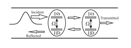
In this paper we study in detail the spatio-temporal distribution of the photon electric field produced by the scattering of a single photon narrow pulse from a system of two identical qubits embedded in a one-dimensional open waveguide (see Fig.1). The method we apply here is the extension of our time-dependent theory that has been developed earlier for the case of a single qubit Green2023 . Our method consists of two steps. First, we rely on the Wigner-Weisskopf approximation in which the rate of spontaneous emission to the guided mode is much less than the qubit frequency, . In this case, a reasonable assumption is to consider the decay rate to be frequency independent taking it at the qubit frequency , . For a system which consists of more than a single qubit the Wigner-Weisskopf approximation is equivalent to Markov approximation which neglects the retardation effects: all qubits feel the scattered field simultaneously. This approximation allows us to obtain the explicit expressions for the forward and backward photon scattering amplitudes. Second, we calculate the associated electric fields, for forward and for backward travelling waves in the whole 1D space: before first qubit, between qubits, and behind the second qubit. The fields consist of several contributions which describe a free field of incoming photon, a spontaneous exponential decay of excited qubits, a slowly decaying part which dies out as the inverse powers of , and a lossless part which represents a steady state solution as . We show that if the distance between qubits is equal to integer of the wavelength , the field energies and exhibit a temporal beatings between the qubit frequency and the photon frequency . The transmittance and reflectance are also obtained from the steady state solution for and , respectively.
Even though our treatment can be applied to real two-level atoms, we consider in our paper an artificial two-level atoms, superconducting qubits operating at microwave frequencies at GHz range. For our calculations we take qubits’ frequency GHz which corresponds to wavelength cm.
The paper is organized as follows. In Section II we present the Jaynes-Cummings Hamiltonian describing the dynamics of two qubits interacting with continuum of modes in a one- dimensional open waveguide. We choose a generic state function on the Hilbert space truncated to the single-excitation subspace. In Section III the general time-dependent equations for qubits’ amplitudes, , , and photon forward, and backward radiation amplitudes are derived for the process when a single-photon pulse is scattered by a system of two identical qubits. The main results of the paper are presented in Section IV where we calculated the spatio-temporal structure of electric field for photon forward and backward travelling waves and discuss the spectral features of the transmitted and reflected waves. Summary of our work is presented in conclusion (Section V). Some technical details of the calculations are given in Appendices A and B.
II The model
We consider two identical qubits in a one- dimensional infinite waveguide with and being the qubit frequency and the distance between them, respectively. On -axis the qubits are located at the points and , respectively.
In the continuum mode representation this system can be described by a Jaynes-Cummings Hamiltonian which accounts for the interaction between qubits and electromagnetic field Blow1990 ; Dom2002 (from now on we use the units throughout the paper, therefore, all energies are expressed in frequency units):
| (1) |
where , is the group velocity of electromagnetic waves, which in our calculations is taken to be the vacuum light speed, m/s; is a photon frequency. is a Pauli spin operator, and are the lowering and raising atomic operators which lower or raise a state of the th qubit. A spin operator .
The photon creation and annihilation operators , , and , describe forward and backward scattering waves, respectively. They are independent of each other and satisfy the usual continuous-mode commutation relations Blow1990 :
| (2) |
The quantity in (1) is the coupling between qubit and the photon field in a waveguide Dom2002 :
| (3) |
where is the off diagonal matrix element of a dipole operator, is the effective transverse cross section of the modes in one-dimensional waveguide. We assume that the coupling is the same for forward and backward waves.
Note that the dimension of the coupling constant is not a frequency, but a square of frequency, , and, as it follows from (2), the dimension of creation and destruction operators is .
Below we consider a single-excitation subspace with either a single photon is in a waveguide and two qubits are in the ground state, or there are no photons in a waveguide with the only one (first or second) qubit in the chain being excited. Therefore, we truncate Hilbert space to the following states:
| (4) |
The Hamiltonian (1) preserves the number of excitations (number of excited qubits + number of photons). In our case the number of excitations is equal to one. Therefore, at any time the system will remain within a single-excitation subspace. It is worth noting here that the Hilbert space is truncated with respect to the number of photons, but the continuum modes are not truncated as was done, for example, in Drob2000 .
The trial wave function of an arbitrary single-excitation state can then be written in the form:
| (5) |
where is the amplitude of th qubit (), and are single-photon amplitudes which are related to a spectral density of forward and backward radiation, respectively.
The function (5) at any time is normalized to unity:
| (6) |
The initial conditions are as follows: all qubits are unexcited at , ; reflected wave is absent, ; transmitted wave , where is the incident pulse which for a single scattering photon is assumed to be normalized to unity, .
We note that as the qubit amplitude , therefore the equation (6) reduces to:
| (7) |
III Equations for qubits’ and photon amplitudes
The Schrodinger equation yields the equations for the amplitudes:
| (8) |
| (9) |
| (10) |
| (11) |
We assume the photon is incident from the left on the first qubit at , so that and . The qubits are assumed to be in the ground state at so that .
| (12) |
| (13) |
| (14) |
| (15) |
In order to obtain analytical solutions for equations (14) and (15) we assume that the qubit amplitudes vary with a rate which is much less than the qubit frequency . Therefore, the qubit amplitudes change little in the time interval over which the remaining part of the integrands have non-zero value . Therefore, we can replace in the integrands by and take them out of the integrals. This is called the Weisskopf-Wigner approximation, which is equivalent to the Markov approximation: dynamics of depends only on time and not on , i.e., the system has no memory of the past.
After some mathematical manipulations (details are given in Appendix A) we arrive at the following equations for qubits’ amplitudes:
| (16) |
| (17) |
where is the rate of spontaneous emission into a waveguide, , .
| (18) |
| (19) |
where
| (20) |
| (21) |
Below for the calculations we use the incident Gaussian pulse:
| (22) |
where is the width of the pulse in the frequency domain.
We assume the Gaussian pulse (22) is sufficiently narrow () so that it can be approximated as a delta pulse Green2023 :
| (23) |
where is the amplitude of incoming wave and is the frequency of the incident photon.
For delta pulse (23) we obtain final expressions for qubits’ amplitudes:
| (24) |
| (25) |
where
| (26) |
The photon radiation amplitudes , are obtained by plugging the expressions (24), (25) for , directly in (12) and (13). The calculations of corresponding integrals in (12) and (13) then yield the following result:
| (27) |
where
| (28) |
| (29) |
where
| (30) |
IV Space-time structure of the scattered field
IV.1 Forward scattering field
The photon wave packet for forward propagating field is given by
| (31) |
where
| (32) |
| (33) |
where is given in (22).
In equations (32) takes any value, both positive and negative, while in equation (33) . In both equations . This condition insures the causality of the forward propagating field which appears at the point not until the signal travels the distance after the scattering. Therefore, the expression (33) describes the field both between the qubits, and behind the second qubit, .
| (36) |
| (37) |
where are given in (21).
| (38) |
| (39) |
IV.1.1 Forward scattering field behind second qubit
First we consider the forward scattering field behind the second qubit, if , where is integer. For this case, the integrals (36), (38) have been calculated in Green2023 :
| (40) |
| (41) |
The integrals and are obtained by replacing with in the expressions for and .
| (42) |
| (43) |
where , , , .
In expressions (40)-(43) the quantities , , and are the exponential integral function, cosine, and sine integrals, respectively, the properties of which are described in Appendix B.
The integrals , are the damping parts of the scattered field which represents spontaneous emission of the excited qubits with the rates , which describe the exponential decay of the corresponding collective states of a two-qubt system. Depending on the value , the damping rates may change from superradiance () to subradiance () emission. The case for which one of the rates equals zero will be considered later.
The integrals , consist of two parts: the time-dependent part which decays as the inverse powers of , and a lossless steady state solution of the scattered field which survives as the time after the scattering tends to infinity. As both the distance from the qubit and the time after the scattering tend to infinity, these scattering fields die out, leaving only the plane-wave stationary solution.
We investigate equation (35) when . In this case, the quantities tend to zero exponentially, while in the quantities the time-dependent terms tend to zero as the inverse powers of . Therefore, for we obtain from (35):
| (44) |
where , .
As a general note to equation (44), we observe that the field behind the second qubit is not zero for finite . As is increased the -dependent part of (44) tends to zero as the inverse power of (see (114) in Appendix B). In principle, the steady state field energy exists in all points of one-dimensional space.
When calculating (44) some caution should be paid if is very near to the qubit location, where cosine integral diverges. This nonphysical effect arises from the point-like model of a qubit adopted in this paper. In order to avoid this effect in all calculations where we study the -dependence of the field, we start the numerics at the distance from a qubit where the influence of cosine integral becomes negligible.
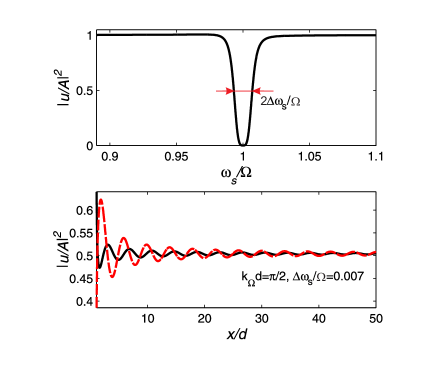
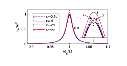
As it follows from (44) spatial effects can persist on the scale of several wavelengthes. We show in Fig.2 the variation of transmitted energy in if the frequency is detuned from the resonance by a half width.
For finite the transmitted energy at resonance () can be obtained directly from (44).
| (45) |
where , .
Even though (46) is derived from (44) for , we will show below that (46) is valid for any value of .
Using the explicit expressions for (26) it is not difficult to show from (46) that in resonance, , far from second qubit the transmitted field is absent, , which is in accordance with the result of quasi stationary theory.
We may compare (46) with the non-Markovian transmission which accounts for retardation effects Green2015 ; Liao2015 :
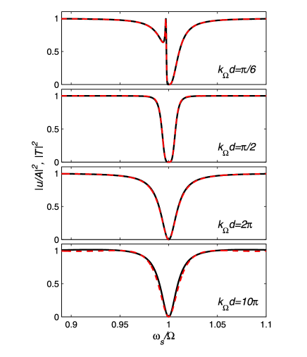
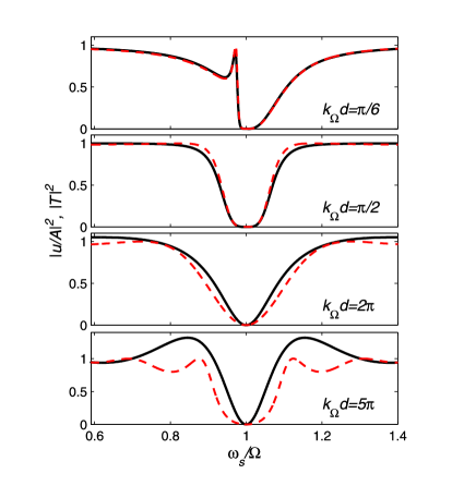
| (47) |
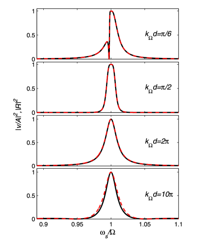
The results of the comparison are shown in Fig.3 and Fig.4. For the frequency dependence (46) practically coincides with that of (47) up to . However, as the value of increases, the departure between two transmittances increases more rapidly and a significant difference is seen for (see Fig.4).
IV.1.2 Forward scattering field behind the second qubit for
In this case, one of the spontaneous rate emissions, is zero. For where is even . For where is odd . Below for definiteness we take where is even number. Then, the photon radiation amplitudes are given by the expressions (28), (29) where
| (48) |
| (49) |
| (50) |
| (52) |
| (53) |
| (54) |
| (55) |
The quantities in (51) are given by the expressions , (40) and , (42) respectively, where is replaced by . The quantities are given in (41) , (43), and the quantities are given by the expressions (41) , (43), respectively, where is replaced by .
We investigate the equation (51) when . In this case, the quantities tend to zero exponentially and in the quantities , the time-dependent terms also tend to zero as the inverse powers of . Therefore, for we obtain from (51) the steady state expression:
| (56) |
where . From (56) we obtain for the equation which describes the dependence of the peak value of the transmitted resonace line on the distance from the second qubit.
| (57) |
where , .
If , all sine and cosine integrals in (56) tend to zero and we obtain for the transmittance the equation (46) where are given in (50). Therefore, the transmittance (46) is valid for any .
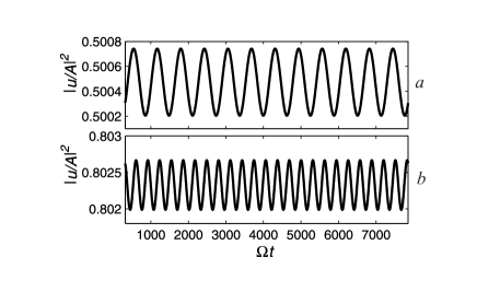
As is seen from (56), at some specific point the field energy exhibits the beatings with the detuning frequency , , and period . The amplitude of these beatings dies out as . The beatings for two detunings are shown in Fig.5 at the distance from the second qubit.
It is not difficult to perform similar calculations for if is odd number. For this case we obtain for the expression which is similar to (51).
| (58) |
IV.2 Backward scattering field
The photon wave packet for backward propagating field is given by
| (60) |
where and .
| (63) |
| (64) |
| (65) |
The integrals and can be obtained from (66) and (67) simply by replacing with in corresponding integrals.
| (68) |
| (69) |
First, we investigate the equation (61) for when . In this case, the quantities tend to zero exponentially and in the quantities the time-dependent terms also tend to zero as the inverse powers of . Therefore, for we obtain from (61):
| (70) |
where .
The reflectance is obtained from (70) in the limit :
| (71) |
Using the explicit expressions for (26) it is not difficult to show that in resonance, , far from the first qubit the reflected field is just the reflected incoming wave, .
| (72) |
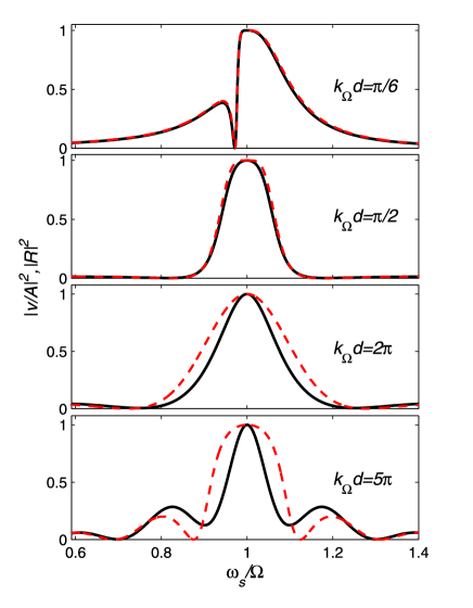
The results of the comparison are shown in Fig.6 and Fig.7. For the frequency dependence (71) practically coincides with that of (72) up to . However, as the value of increases, the departure between two transmittances becomes significant for (see Fig.7).
For finite the reflectance at resonance can be obtained directly from (70):
| (73) |
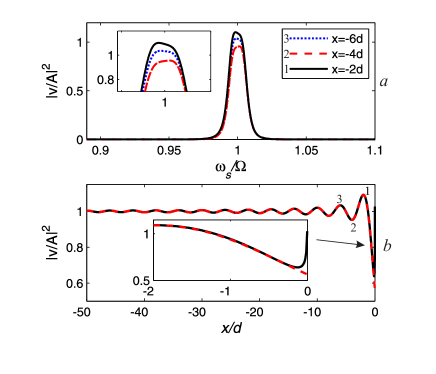
As is seen from (73) the peak value of resonance line depends on specific -position. This is shown in Fig.8, upper panel, where three resonance lines calculated from (70) are shown for , respectively. The dependence of the peak value on calculated from (73) is shown in the lower panel in Fig.8. We see that at some the peak value of resonance line may exceed unity (black solid line in Fig.8, panel (a)). It is not related to the divergence of at small as is shown in the inset in Fig.8, panel (b) where the dashed red line is calculated from (73) with being neglected. The peak value which is higher than unity at a single frequency and a single spatial point does not contradict the energy conservation, which should account for the whole frequency range and whole volume. The origin of the higher-than-unity peak comes mainly from the interference term in (73).
Next, we analyze the reflected field for , where is the integer. For even the quantities are given in (50) and we obtain for reflected wave the expression which is similar to (51):
| (74) |
where
| (75) |
| (76) |
| (77) |
The expressions for can be obtained from equations (75), (76), (77) by replacing with in corresponding equations.
The quantities in (74) are given by the expressions (66) and (68), where is replaced by . The quantities are given in (67) (69), and the quantities are given by the expressions (67), (69) where is replaced by .
We investigate the equation (74) when . In this case, the quantities tend to zero exponentially and in the quantities , the time-dependent terms also tend to zero as the inverse powers of . Therefore, for we obtain from (74):
| (78) |
where , . From (78) we obtain for the equation which describes the dependence of the peak value of the reflected resonace line on the position point .
| (79) |
where where , .
If , all sine and cosine integrals in (78) tend to zero and we obtain for the reflectance the equation (71) where are given in (50).
Reflected resonance lines for and several , calculated from (78) for c are shown in Fig.9. A small amplification of the resonance peak (line 1 in Fig.9) is due to the influence of the interference term in the first line in (79). Similar effect is known in Fabry-Perot interferometer with semitransparent mirrors where the strength mode of electric field can significantly exceed the amplitude of the input field Ley1987 . This amplification effect will be discussed in more detail at the end of this section.
It is not difficult to perform similar calculations for if is odd number. For this case we obtain for the expression which is similar to (74).
| (80) |
where are given in (59).
In the limit we obtain from (80) the expression which is analogous to equation (78) with the only exception: in the third line in (78) should be replaced with .
As in the -even case, the reflectance here is also given by the expression (71).
IV.3 Scattering waves between the qubits
Between qubits, , the photon field is a superposition of the forward and backward travelling waves.
| (81) |
The general expressions for and are given in (35) and (61) where . First we consider the case , so that in expressions (35) and (61) we neglect the terms , , and , which tend exponentially to zero as .
| (82) |
| (83) |
In these equations , and .
In (82) the quantity where is given in (41). The calculation of where provides the following result (see expression (123) in the Appendix B):
| (84) |
Next, in the expressions (41) and (84) we neglect the terms which are tend to zero as the inverse powers of . Therefore, for interqubit forward travelling wave we obtain:
| (85) |
where . Now we calculate the interqubit backward travelling wave. In equation (83) the quantity is given by the equation (69). The calculation of for yields the following result (see expression (127) in the Appendix B):
| (86) |
In the expressions (69) and (86) we neglect the terms which are tend to zero as the inverse powers of . Therefore, for interqubit backward travelling wave we obtain:
| (87) |
where . From (85) and (87) we obtain for the interqubt field energy at the resonance point the following simple expression:
| (88) |
where , .
The behavior of the photon field between qubits calculated from (85) and (87) is shown in Fig.10 for . In the upper panel the resonance lines are shown for three spatial points, , , and . In the lower panel the dependence of the field energy on is shown for several values of the photon frequency, , , , ; . , GHz, m.
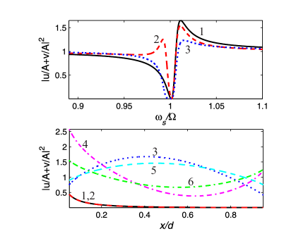
In Fig.10 we observe a significant amplification of the field energy for some spatial points and some frequencies. We discuss this effect in a more detail in the end of this section.
IV.3.1 Interqubit field for
Below for definiteness we take where is even number. In this case, the interqubit forward and backward travelling waves, and are given by the equations (51), (74) where and , and are defined in (50). Neglecting in these equations the exponential decaying terms we obtain:
| (89) |
| (90) |
In (89) the quantities where , and where are given in (41) and (84), respectively. The integrals where and where are given by the expressions (122) and (123), respectively, where should be replaced with .
| (91) |
where , .
| (92) |
where , .
Therefore, when for interqubit forward scattering field we obtain:
| (93) |
where , .
In equation (90) which describes the backward scattering field between qubits the integral where is given in (86), the integral is given by the equation (69), and the integral is given by the expression (127) where should be replaced with :
| (94) |
where , .
The integral is obtained from the expression (126) where should be replaced with , and should be replaces with :
| (95) |
where , .
Therefore, when for interqubit backward scattering field we obtain:
| (96) |
Between the qubits the photon field is a superposition of the forward, (93), and backward, (96) travelling waves.
The behavior of the photon field between qubits calculated from (93) and (96) for and c is shown in Fig.11. In the upper panel the resonance lines are shown for three spatial points, (1;black solid line), (2; red dashed line), (3;dotted-dashed blue line). In the lower panel the dependence of the field energy on is shown for several values of the photon frequency, (1) ; (2) ; (3) ; (4) ; (5) .
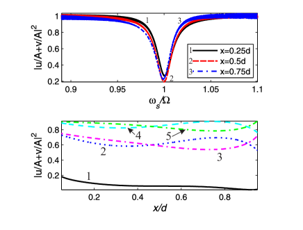
If we compare the forms of resonance lines and the peak values in Fig.10 with those in Fig.11 we observe a drastic difference. For example, a significant amplification of the field energy for some spatial points and frequencies is seen in Fig.10. We attribute this difference to the constructive interference between the radiation of symmetric and asymmetric states of a two-qubit system. For both these states are not decoupled from the waveguide photons. If (Fig.11) the asymmetric state is decoupled from the photon field and, therefore, does not contribute to the radiation.
V Conclusion
In summary, we have developed the time-dependent theory of the scattering of a narrow single-photon Gaussian pulse from a two-qubit system embedded in 1D open waveguide. The theory is valid for Markov approximation when time delay effects between qubits are neglected. This approximation allows us to obtain explicit analytical expressions for the forward and backward travelling waves, their spatial and temporal distribution. We show that the scattered fields consist of several parts: a free field of incoming photon, the part which describes a spontaneous exponential decay of excited qubits, a slowly decaying part dying out as the inverse powers of , which is the manifestation of subradiant emission, and a lossless part which represents a steady state solution as . We systematically compare the transmittance and reflectance for our model with those for non-Markovian case which are known from the literature. It turned out that our transmittance and reflectance work well for if . If the interqubit distance is equal to wavelength or half wavelength of resonance frequency, the field energy exhibits the beatings with the detuning frequency .
Our calculations show that spatial effects can persist on the scale of several ’s (see Fig.2 and Fig.8). For on-chip realization this length is not small compared with the dimensions of a superconducting qubit (typically several microns). The power of microwave signal is so low that the use of linear amplifiers for the detection of the qubit signal is a common practice. The current opportunity for on-chip realization of superconducting qubits with associated circuitry allows for the placement of the amplifier within the order of the wavelength from the qubits Lec2021 . Therefore, in microwave range the near-field effects can in principle be detectable.
We believe that the results obtained in this paper may have some practical applications in quantum information technologies including single-photon detection in a microwave domain as well as the optimization of the control and readout of a qubit’s quantum state.
Acknowledgments. The authors thank O. V. Kibis and A. N. Sultanov for fruitful discussions. The work is supported by the Ministry of Science and Higher Education of Russian Federation under the project FSUN-2023-0006.
Author contributions. YSG wrote the manuscript and contributed to its theoretical interpretation. AAS and AGM performed analytical calculations and computer simulations. All authors discussed the results and commented on the manuscript. The authors declare that they have no competing interests.
Data Availability Statement. The manuscript has no associated data in a public repository.
Appendix A Derivation of equations for qubits’ amplitudes (16), (17)
| (98) |
where
| (99) |
Next, we change variables in (99), , and tend the upper bound of integral to infinity.
| (100) |
where denotes Cauchy’s principal value.
| (102) |
The quantity results in the shift of the qubit frequency . We assume the shift is small and include it implicitly in the definition of . As the coupling between qubit and the field is effective at the qubit resonance, we take it off the Cauchy principal integral in equations (101), (102) at the qubit resonance frequency. Then for the Cauchy principal integral we obtain:
| (103) |
For two-qubit system the rate of spontaneous emission can be found from Fermi’s golden rule:
| (104) |
Appendix B Properties of sine and cosine integrals and some related integrals
| (107) |
| (108) |
where is defined on the whole real axis, while is defined only for .
Using these definitions it is not difficult to show that
| (109) |
| (110) |
From definitions (105), (106), and (107) the parity relations follow:
| (112) |
The exponential integral in the expressions (40), (42) is defined as follows Abram1964 :
| (113) |
The behavior of scattered fields at large x and t follows from the asymptote of the exponential integral function, sine, and cosine integrals Grad2007 ; Jahnke :
| (114) |
where .
| (115) |
where .
Below we illustrate the application of above formulae for the calculation of some integrals which we use throughout the paper.
| (116) |
This integral, where and describes the forward travelling wave between qubits as well as behind the second qubit, .
Changing the variables in the integrand of (116), , , we obtain
| (117) |
The calculation of the first integral in (117) yields:
| (118) |
Similar expression we obtain for second integral in (117):
| (119) |
Therefore, for we obtain:
| (120) |
Using the relation (111) we rewrite (120) as follows:
| (121) |
Here , and . Therefore, we obtain:
| (122) |
where , .
For integral which describes the forward travelling wave between qubits, we obtain from (121), where is replaced with :
| (123) |
where , .
Next, we consider the integral (64) which describes the backward travelling wave in front of the first qubit .
| (124) |
where , .
The calculation of this integral is similar to that of . For we obtain the following result:
| (125) |
Therefore, for we finally obtain:
| (126) |
where , .
There are two integrals which describe the backward travelling wave between qubits, where , and where . The quantity with follows from (125) where :
| (127) |
where , .
The integral is obtained from equation (126) where is replaced with , and where , .
References
- (1) J. M. Raimond, M. Brune, and S. Haroche, Manipulating quantum entanglement with atoms and photons in a cavity, Rev. Mod. Phys. 73, 565 (2001)., 565 (2001).
- (2) D. Roy, C. M. Wilson, and O. Firstenberg, Strongly interacting photons in one-dimensional continuum Rev. Mod. Phys. 89, 021001 (2017).
- (3) A. S. Sheremet, M. I. Petrov, I. V. Iorsh, A. V. Poshakinskiy, and A. N. Poddubny, Waveguide quantum electrodynamics: Collective radiance and photon-photon correlations. Rev. Mod. Phys. 95, 015002 (2023).
- (4) P. Krantz, M. Kjaergaard, F. Yan, T. P. Orlando, S. Gustavsson, and W. D. Oliver, A quantum engineer’s guide to superconducting qubits. Appl. Phys. Rev. 6, 021318 (2019).
- (5) X. Gu, A. F. Kockum, A. Miranowicz, Y.-X. Liu, and F. Nori, Microwave photonics with superconducting quantum circuits, Phys. Rep. 718, 1 (2017).
- (6) M. Kjaergaard, M. E. Schwartz, J. Braumüller, P. Krantz, Joel I.-J. Wang, S. Gustavsson, and W. D. Oliver, Superconducting qubits: current state of play. Ann. Rev. Condensed Matter Phys. 11, 369 (2019).
- (7) J. Ruostekoski and J. Javanainen, Arrays of strongly coupled atoms in a one-dimensional waveguide. Phys. Rev. A 96, 033857 (2017).
- (8) K. Lalumi‘ere, B. C. Sanders, A. F. van Loo, A. Fedorov, A. Wallraff, and A. Blais, Input-output theory for waveguide QED with an ensemble of inhomogeneous atoms. Phys. Rev. A 88, 043806 (2013).
- (9) D. E. Chang, L. Jiang, A. V. Gorshkov, and H. J. Kimble, Cavity QED with atomic mirrors. New J. Phys. 14, 063003 (2012).
- (10) M. Mirhosseini, E. Kim, X. Zhang, A. Sipahigil, P. B. Dieterle, A. J. Keller,A. Asenjo-Garcia, D. E. Chang, and O. Painter, Cavity quantum electrodynamics with atom-like mirrors. Nature 569, 692 (2019).
- (11) J. D. Brehm, A. N. Poddubny, A. Stehli, T. Wolz, H. Rotzinger, and A. V. Ustinov, Waveguide bandgap engineering with an array of superconducting qubits, npj Quantum Materials 6, 10 (2021).
- (12) A. F. van Loo, A. Fedorov, K. Lalumi‘ere, B. C. Sanders, A. Blais, and A. Wallraff Photon-mediated interactions between distant artificial atoms. Science 342, 1494 (2014).
- (13) J.-T. Shen and S. Fan, Theory of single-photon transport in a single-mode waveguide. I. Coupling to a cavity containing a two-level atom. Phys. Rev. A 79, 023837 (2009).
- (14) M.-T. Cheng, J. Xu, and G. S. Agarwal, Waveguide transport mediated by strong coupling with atoms. Phys. Rev. A 95, 053807 (2017).
- (15) Y.-L. L. Fang, H. Zheng, and H. U. Baranger, One-dimensional waveguide coupled to multiple qubits photon-photon correlations. EPJ Quantum Technol. 1, 3 (2014).
- (16) H. Zheng and H. U. Baranger, Persistent Quantum Beats and Long-Distance Entanglement from Waveguide-Mediated Interactions. Phys. Rev. Lett. 110, 113601 (2013).
- (17) D. Roy, Correlated few-photon transport in one-dimensional waveguides: Linear and nonlinear dispersions, Phys. Rev. A 83, 043823 (2011).
- (18) J.-F. Huang, T. Shi, C. P. Sun, and F. Nori, Controlling single-photon transport in waveguides with finite cross section, Phys. Rev. A 88, 013836 (2013).
- (19) G. Diaz-Camacho, D. Porras, and J. J. Garcia-Ripoll, Photon-mediated qubit interactions in one-dimensional discrete and continuous models. Phys. Rev. A 91, 063828 (2015).
- (20) S. Fan, S. E. Kocabas, and J.-T. Shen, Input-output formalism for few-photon transport in one-dimensional nanophotonic waveguides coupled to a qubit, Phys. Rev. A 82, 063821 (2010).
- (21) A. H. Kiilerich and K. Molmer, Input-Output Theory with Quantum Pulses. Phys. Rev. Lett. 123, 123604 (2019).
- (22) Ya. S. Greenberg and A. A. Shtygashev, Non hermitian Hamiltonian approach to the microwave transmission through a one-dimensional qubit chain. Phys.Rev. A 92, 063835 (2015).
- (23) Ya. S. Greenberg, A. A. Shtygashev, and A. G. Moiseev, Waveguide band-gap N-qubit array with a tunable transparency resonance. Phys.Rev. A 103, 023508 (2021).
- (24) T. S. Tsoi and C. K. Law, Quantum interference effects of a single photon interacting with an atomic chain. Phys. Rev. A 78, 063832 (2008).
- (25) Y. Chen, M. Wubs, J. Mork, and A. F. Koendrink, Coherent single-photon absorption by single emitters coupled to one-dimensional nanophotonic waveguides, New J. Phys. 13,103010 (2011).
- (26) Z. Liao, X.Zeng, S.-Y. Zhu, and M. S. Zubairy, Single-photon transport through an atomic chain coupled to a one-dimensional nanophotonic waveguide. Phys. Rev. A92, 023806 (2015).
- (27) Z. Liao, H. Nha, and M. S. Zubairy, Dynamical theory of single-photon transport in a one-dimensional waveguide coupled to identical and nonidentical emitters. Phys. Rev. A 94, 053842 (2016).
- (28) Z. Liao, X. Zeng, H. Nha, and M. S. Zubairy, Photon transport in a one-dimensional nanophotonic waveguide QED system Phys. Scr. 91, 063004 (2016).
- (29) C. Zhou, Z. Liao, and M. S. Zubairy, Decay of a single photon in a cavity with atomic mirrors. Phys. Rev. A 105, 033705 (2022).
- (30) Ya. S. Greenberg and A. A. Shtygashev, The pulsed excitation in two-qubit systems. Phys. Solid State 60, 2109 (2018).
- (31) P. Domokos, P. Horak, and H. Ritsch, Quantum description of light-pulse scattering on a single atom in waveguides. Phys. Rev. A 65, 033832 (2002).
- (32) Ya. S. Greenberg, A. G. Moiseev, and A. A. Shtygashev, Single-photon scattering on a qubit: Space-time structure of the scattered field. Phys. Rev. A 107, 013519 (2023).
- (33) F. Lecocq, F. Quinlan, K. Cicak, J. Aumentado, S. A. Diddams, J. D. Teufel, Control and readout of a superconducting qubit using a photonic link. Nature 591, 575 (2021).
- (34) K. J. Blow, R. Loudon, and S. J. D. Phoenix, Continuum fields in quantum optics. Phys. Rev. A 42, 4102 (1990).
- (35) G. Drobny, M. Havukainen, and V. Buzek, Stimulated emission via quantum interference Scattering of one-photon packets on an atom in a ground state. J. Mod. Optics 47, 851 (2000).
- (36) M. Ley and R. Loudon, Quantum theory of high resolution length measurement with a Fabry-Perot interferometer, J. Mod. Opt. 34, 227 (1987).
- (37) M. Abramowitz and I. A. Stegun, Handbook of Mathematical Functions with Formulas, Graphs, and Mathematical Tables, NIST, 1964.
- (38) I. S. Gradshteyn and I. M. Ryzhik Table of Integrals, Series, and Products. Elsevier Inc. 7-th ed. Amsterdam 2007, 1220 pages.
- (39) E. Jahnke, F. Emde, F. Lösch, Tables of higher functions. 1965, 7th ed.