Robust Offline Policy Evaluation and Optimization with Heavy-Tailed Rewards

Abstract

This paper endeavors to augment the robustness of offline reinforcement learning (RL) in scenarios laden with heavy-tailed rewards, a prevalent circumstance in real-world applications. We propose two algorithmic frameworks, ROAM and ROOM, for robust off-policy evaluation (OPE) and offline policy optimization (OPO), respectively. Central to our frameworks is the strategic incorporation of the median-of-means method with offline RL, enabling straightforward uncertainty estimation for the value function estimator. This not only adheres to the principle of pessimism in OPO but also adeptly manages heavy-tailed rewards. Theoretical results and extensive experiments demonstrate that our two frameworks outperform existing methods on the logged dataset exhibits heavy-tailed reward distributions.

Keywords: Offline reinforcement learning, heavy-tailed rewards, median of mean, uncertainty qualification

1 Introduction

In reinforcement learning (RL, Sutton and Barto, 2018), evaluating and optimizing policies without accessing the environment becomes crucial nowadays, because frequently interacting with the environment could be prohibitively expensive or even impractical in many real-world applications such as robotics, healthcare, education, autonomous driving, and so on. This leads to a surge of interest in offline RL (Levine et al., 2020; Uehara et al., 2022), which aims to leverage only logged data for policy evaluation and optimization.

The success of offline RL so far crucially relies on that the reward distribution is well-behaved. However, in a number of real-world applications, the reward distribution is usually heavy-tailed. Heavy-tailed rewards can be generated by various real-world decision-making systems, such as the stock market, networking routing, scheduling, hydrology, image, audio, and localization errors, etc. (Georgiou et al., 1999; Hamza and Krim, 2001; Huang and Zhang, 2017; Ruotsalainen et al., 2018).

The heavy-tailedness pose great challenges to existing offline RL methods. We illustrate this via a fundamental problem in offline RL: off-policy evaluation (OPE). OPE aims to evaluate the value of policies using only logged data. One classic algorithm is fitted-Q evaluation (FQE), where each step is solving a regression problem with the response variable being the observed reward plus some estimated long-term values. Yet, it is well-known that the performance of standard regression methods is very sensitive to heavy-tailed responses (Lugosi and Mendelson, 2019) and will have a much slower convergence rate. Consequently, this issue will degrade the performance of policy evaluation. The heavy-tailed rewards pose even more challenges to offline policy optimization (OPO), because the issue of overestimation in standard RL algorithms could be aggravated. In addition, many recent advances in OPE rely on accurate uncertainty quantification such as confidence intervals (Jin et al., 2021), which could be unreasonably wide due to the heavy-tailed distributions.

To accommodate the heavy-tailed rewards in offline RL, we propose new frameworks for both OPE and OPO by leveraging the median-of-means (MM) estimator in robust statistics (Nemirovskij and Yudin, 1983; Alon et al., 1996). Specifically, we design a few frameworks that can effectively robustify existing RL algorithms against the heavy-tailed rewards. The procedures are simple and easy-to-implement. Moreover, the proposed approach also provides a natural way for qualifying the uncertainty of value estimation, which is crucial in both OPE and OPO.

Contribution. The contribution of this paper is three-fold. First, we propose a general and unified framework to improve the robustness of existing OPE and OPO methods against heavy-tailed rewards. By leveraging MM, our approach naturally allows uncertainty quantification of the estimated values. This is critical for OPE in high-risk applications (e.g., healthcare) and also for OPO to incorporate the principle of pessimism (Jin et al., 2021; Bai et al., 2022) to address insufficent data coverage.

Second, we provide rigorous theoretical analyses on our OPE and OPO algorithms and clearly demonstrate their advantages over existing solutions that ignore the heavy-tailed issue. In particular, our analysis only requires the reward to have finite $(1+\alpha)$th moment. On the contrary, most of the existing methods require the rewards to be bounded (or sub-Gaussian) to achieve similar performance.

Finally, on a couple of benchmark OpenAI environments, we observe the superiority of the proposed algorithms against existing ones when the rewards are heavy-tailed. In particular, for OPE, our methods are 1.5 to 30 times more accurate than the non-robust algorithms in terms of rooted MSE; on several D4RL benchmarks for OPO, the score of the robust version is about 1.3 to 3 times higher than those of the vanilla version of state-of-the-art (SOTA) algorithm.

2 Related Works

Off-Policy Evaluation. In the literature, there are three commonly-used approaches for OPE. The first one is the direct method (DM), which evaluates the target policy by estimating its Q-function (Bertsekas, 2012; Farajtabar et al., 2018; Sutton and Barto, 2018; Le et al., 2019; Duan et al., 2020; Liao et al., 2021). Importance sampling (IS) is another popular OPE approach (Precup, 2000; Thomas et al., 2015; Liu et al., 2018; Hanna et al., 2019; Nachum et al., 2019; Xie et al., 2019; Dai et al., 2020; Wang et al., 2021), motivated by the change of measure theorem. Sequential IS gives an unbiased estimator but has an exponentially large variance with respect to the horizon. Liu et al. (2018); Xie et al. (2019) developed marginal IS estimators to break this curse of horizon. The last approach aims to exploit the advantages of both DM and IS, by combining them to derive a doubly robust (DR) estimator (Thomas and Brunskill, 2016; Jiang and Li, 2016; Farajtabar et al., 2018; Tang et al., 2019; Kallus and Uehara, 2020; Shi et al., 2021; Liao et al., 2022). We refer to Uehara et al. (2022) for a comprehensive review for OPE. However, to our knowledge, most existing methods cannot handle the heavy-tailed issue.

Offline Policy Optimization. It is well-known that standard OPO methods (e.g., Ernst et al., 2005) may fail to converge and produce unstable solutions due to the distributional mismatch in the offline setting (Wang et al., 2021). To address this limitation, one possible approach is to force the learned policy to choose actions close to the observed ones in the offline data (Wu et al., 2020; Brandfonbrener et al., 2021; Fujimoto and Gu, 2021; Kostrikov et al., 2021; Dadashi et al., 2021). Recently, there is a streamline of research utilizing either the principle of pessimism (e.g., Kumar et al., 2020; An et al., 2021; Jin et al., 2021; Xie et al., 2021; Yin et al., 2021; Yu et al., 2021; Bai et al., 2022; Fu et al., 2022; Guo et al., 2022; Shi et al., 2022; Uehara and Sun, 2022; Lyu et al., 2022) or in-sample learning (Kostrikov et al., 2022; Fu et al., 2022; Xu et al., 2023; Zhang et al., 2023) to address the insufficient data coverage issue. We refer interested readers to Prudencio et al. (2023) for a recent survey on OPO. However, there is no existing OPO methods that can handle the heavy-tailed rewards.

Robust RL. Most existing works on handling heavy-tailed rewards are only designed for bandits, a special case of RL. Various robust mean estimators are proposed for designing algorithms in finding an optimal arm in the online setting (e.g., Bubeck et al., 2013; Shao et al., 2018; Lu et al., 2019; Zhong et al., 2021). However, less attention has been paid to heavy-tailed rewards when there is state transition. To the best of our knowledge, Zhuang and Sui (2021) is the most related paper studying this issue. They focus on an online setting which is substantially different from our offline setting. Moreover, Zhuang and Sui (2021) directly applies robust mean estimators to the reward function itself and focuses on tabular settings. In contrast, our proposed framework allows continuous state-action spaces.

We remark that there has another line of research on robust offline RL (Chen et al., 2021; Lykouris et al., 2021; Mo et al., 2021; Si et al., 2020; Zhang et al., 2021; Kallus et al., 2022; Xu et al., 2022; Zhang et al., 2022), which mainly focuses on robust decision making under the uncertainty of the changing environment. Another stream studies OPE/OPO under the robust Markov decision process (Nilim and El Ghaoui, 2005) by exploiting prior distributional information allow uncertainty quantification (Mannor et al., 2016; Wiesemann et al., 2013; Wang et al., 2022; Goyal and Grand-Clement, 2023). These goal are different from ours.

3 Preliminaries

Markov decision process. We consider an infinite-horizon discounted stationary Markov Decision Process (MDP, Sutton and Barto, 2018), which is defined by a tuple $\mathcal{M}\coloneqq(\mathcal{S},\mathcal{A},\mathcal{P},\mathcal{R},\gamma)$ where $\mathcal{S}$ is the state space, $\mathcal{A}$ is the action space, the transition kernel $\mathcal{P}(\bullet|S_{t-1},A_{t-1})$ specifies the probability mass (or density) function of $S_{t}$ by taking action $A_{t-1}$ at a state $S_{t-1}$, and similarly $\mathcal{R}$ specifies the reward. The constant $\gamma\in[0,1)$ is the discount factor. We denote the initial state distribution as $\mathbb{G}$. For simplicity of notations, we assume $\mathbb{G}$ is pre-specified in this paper. $\mathbb{G}$ can be estimated from the empirical initial state distribution in practice.

In the existing literature, the reward is assumed to be uniformly bounded or at least sub-Gaussian (Thomas and Brunskill, 2016; Fan et al., 2020; Shi et al., 2021; Chen and Qi, 2022). However, as discussed in the introduction, such an assumption could be violated in many real applications. In this paper, we consider a much milder assumption, that is, the reward distribution $\mathcal{R}$ has finite $(1+\alpha)$-th moments for some $\alpha\in(0,1]$. Then, the mean reward function $r(s,a)=\mathbb{E}(R_{t}|S_{t}=s,A_{t}=a)$ exists. No other assumptions are imposed and the reward distribution can be arbitrarily heavy-tailed. Let $\pi(a|s):\mathcal{S}\rightarrow\mathcal{A}$ be a given policy that specifies the conditional distribution of the action given the state. We next the value function $V^{\pi}(s)\coloneqq\mathbb{E}^{\pi}\left[\sum_{t=0}^{\infty}\gamma^{t}R_{t}\mid S_{0}=s\right]$ and the Q-function $Q^{\pi}(s,a)\coloneqq\mathbb{E}^{\pi}\left[\sum_{t=0}^{\infty}\gamma^{t}R_{t}\mid S_{0}=s,A_{0}=a\right]$. Let $\mathbb{E}_{\mathcal{D}}[\cdot]$ denote the expectation taken with respect to the empirical measure over the offline data $\mathcal{D}$.

Problem Formulation. We assume that an agent interacts with the environment $\mathcal{M}$ and collects a series of random tuples in the form of $(S,A,R,S^{\prime})$ using one behavior policy. The offline dataset $\mathcal{D}$ consists of all tuples with form $(S,A,R,S^{\prime})$. There are two main tasks in offline RL as follows.

• Off-policy evaluation (OPE): given the offline dataset $\mathcal{D}$ and a given target policy $\pi$, OPE estimates its value $\eta^{\pi}\coloneqq{\mathbb{E}}_{s\sim\mathbb{G},a\sim\pi(\bullet|s)}Q^{\pi}(s,a)$.

• Offline policy optimization (OPO): given the offline dataset $\mathcal{D}$, OPO aims to learn an optimal policy ${\pi}^{*}=\arg\max_{\pi}\eta^{\pi}$.

Most existing methods for the two tasks crucially rely on the assumption that the rewards are uniformly bounded, yet simply employing them cannot address the challenges posed by heavy-tailed rewards, as illustrated in the example below.

Failure of standard direct methods. To illustrate, we mainly focus on DM for OPE, which has shown promising performances from theory and empirical studies (Duan et al., 2020; Voloshin et al., 2021). A DM-type OPE algorithm first estimates the Q-function as $\hat{Q}$ and then estimate the value of $\eta^{\pi}$ by constructing a plug-in estimator for $\hat{\eta}^{\pi}=\mathbb{E}_{s\sim\mathbb{G},a\sim\pi(\bullet|s)}\hat{Q}^{\pi}(s,a)$.

To see the failure of DM, we first present the connection between $\mathrm{Q}$-function estimation and population mean estimation. Define the conditional discounted state-action visitation distribution of the tuple $(s,a)$ following policy $\pi$ starting from $(s_{0},a_{0})$ as $d^{\pi}\left(a,s|a_{0},s_{0}\right)=(1-\gamma)\{\mathbb{I}(a=a_{0},s=s_{0})+\sum_{t=1}^{\infty}\gamma^{t}p_{t}^{\pi}\left(a,s\mid a_{0},s_{0}\right)\}$. Then,

$$\begin{aligned} Q^{\pi}(s_{0},a_{0})&=(1-\gamma)^{-1}\mathbb{E}_{\left(S_{t},A_{t}\right)\sim d^{\pi}\left(a,s\mid a_{0},s_{0}\right),R_{t}\sim\mathcal{R}\left(S_{t},A_{t}\right)}R_{t}.\end{aligned}$$

In other words, the Q-value $Q^{\pi}\left(s_{0},a_{0}\right)$ is the population mean of the stochastic rewards under the corresponding state-action visitation distribution induced by policy $\pi$ starting from $\left(s_{0},a_{0}\right)$. The heavy tailedness of $R_{t}$ typically will carry over to the distribution of $\sum_{t=0}^{\infty}\gamma^{t}R_{t}$ conditioned on $\left\{S_{0}=s,A_{0}=a\right\}$ and following $\pi$. In this sense, the estimation of $Q^{\pi}\left(s_{0},a_{0}\right)$ will face the same challenge as the population mean estimation with heavy-tailed noises. At this case, the estimation error of the sample mean $\bar{R}$ can be upper bounded by $|\bar{R}-\mu|\leq C^{\prime}\delta^{-\frac{1}{1+\alpha}}n^{-\frac{\alpha}{1+\alpha}}$ with probability at least $1-\delta$, for a constant $C^{\prime}>0$. To ensure a high-probability result, $\delta$ shall inversely scale polynomially in $n$, causing the error bound may scale polynomially in $n$, which dominate the (constant) reward means.

Median-of-mean method. The key tool in our algorithms is the MM estimator (Nemirovskij and Yudin, 1983; Alon et al., 1996) in robust statistics. Due to its flexibility and that it is straightforward to produce uncertainty quantification, MM has also been employed in robust linear regressions as well (Zhang and Liu, 2021; Minsker, 2015). We present its form in population mean estimation and related property below.

Definition 1 (Population mean estimation via MM).

Let $R_{1},\ldots,R_{n}$ be $n$ i.i.d. real-valued heavy-tailed observations under a distribution $F$. To estimate the population mean, we first partition $[n]=\{1,\ldots,n\}$ into $K\in\mathbb{N}^{+}$blocks $B_{1},\ldots,B_{K}$, each of size $\left|B_{i}\right|\geq\lfloor n/K\rfloor\geq 2$. We compute the sample mean in each block as $Z_{k}=\frac{1}{\left|B_{k}\right|}\sum_{i\in B_{k}}R_{i}$. The MM estimator for the mean value of $F$ is defined as $\operatorname{Median}\left(\left\{Z_{1},\ldots,Z_{K}\right\}\right)$.

Proposition 1 (Lugosi and Mendelson (2019), Theorem 3).

Suppose $R_{1},\ldots,R_{n}$ are i.i.d. with mean $\mu$ and the $(1+\alpha)$ th moment. For any $\delta\in(0,1)$, by setting $K=\lceil 8\log(2/\delta)\rceil$, we have with probability at least $1-\delta$ that

$$\left|\widehat{\mu}_{n}-\mu\right|\leq C[\log(1/\delta)]^{\frac{\alpha}{1+\alpha}}n^{-\frac{\alpha}{1+\alpha}}$$

for some constant $C>0$.

Comparing sample mean and the MM, we easily see that sample mean’s dependence on the confidence parameter $\delta$ is exponentially worse than that of MM. Indeed, a sub-Gaussian assumption is typically required for sample mean to enjoy the same property as $\mathrm{MM}$ estimator. Based on the aforementioned discussion, we will borrow ideas from the MM to improve the robustness of OPE and OPO.

4 MM for Robust Offline RL

In this section, we start by presenting our proposal for OPE to illustrate the main idea of utilizing MM in offline RL to address the heavy-tailed rewards. We then extend the idea to OPO in Section 4.2.

4.1 MM for OPE

This section introduces the Robust Off-policy evaluAtion via Median-of-means (ROAM) framework. For ease of exposition, we first focus on the DM in this paper. Specifically, the discussions above motivate us to consider leveraging the MM scheme for robust estimation of $Q^{\pi}$ (see an illustration in Figure 1). We first split all trajectories $\mathcal{D}$ into $K$ partitions $\left\{\mathcal{D}_{k}\right\}_{k=1}^{K}$. Notice that data subsets across the $K$ splits are i.i.d. Next, with any given DM-type OPE algorithm BaseOPE, we obtain $K$ i.i.d. estimates $\{\widehat{Q}_{k}^{\pi}\}_{k=1}^{K}$ for $Q^{\pi}$. However, with heavy-tailed rewards, these estimates may also have large errors and distributed with heavy tails around $Q^{\pi}$. As discussed above, this is similar to the sample average in every split for population mean estimation. Therefore, we propose to extend MM to OPE by first applying the median operator to the $K$ Q-functions and then calculate the integrated value estimate as $\widehat{\eta}^{\pi}=\mathbb{E}_{s\sim\mathbb{G},a\sim\pi(\bullet|s)}\operatorname{Median}(\{\widehat{Q}_{k}^{\pi}(s,a)\}_{k=1}^{K})$. We summarize the procedure in Algorithm 1. Notably, our approach employs a split-and-aggregation strategy to estimate a robust Q function, which is markedly different from the standard MM method for estimating a scalar. As such, verifying the robustness of the estimated Q function necessitates a non-trivial analysis of the proposed procedure.

Figure 1: Graphical illustration for ROAM. $Q_{\mathrm{MM}}(s,a)$ is equal to $\operatorname{Median}(\{\widehat{Q}_{k}^{\pi}(s,a)\}_{k=1}^{K})$.

Algorithm 1 Robust Off-policy Evaluation via Median-of means based Direct Method (ROAM-DM)

1:Policy $\pi$, data $\mathcal{D}$, data partitions number $K$, decay rate $\gamma$, base DM-type OPE algorithm BaseOPE

2:Partition trajectories $\mathcal{D}$ into $K$ disjoint parts: $\mathcal{D}_{1},\ldots,\mathcal{D}_{K}$.

3:for $k=1,\ldots,K$ do

4:     $\widehat{Q}_{k}^{\pi}\leftarrow\texttt{BaseOPE}\left(\pi,\mathcal{D}_{k},\gamma\right)$

5:end for

6:$\widehat{\eta}^{\pi}\leftarrow\mathbb{E}_{s\sim\mathbb{G},a\sim\pi(\bullet|s)}\text{Median}(\{\widehat{Q}_{k}^{\pi}(s,a)\}_{k=1}^{K}).$

7:$\widehat{\eta}^{\pi}.$

Uncertainty quantification. In many high-risk applications such as mobile health studies, in addition to a point estimate on a target policy’s value, it is crucial to quantify the uncertainty of the value estimates, which has attracted increasing attention in recent years (Dai et al., 2020; Shi et al., 2021; Liao et al., 2021, 2022; Kallus et al., 2022). One prominent advantage of leveraging MM in OPE is that it is straightforward to produce uncertainty quantification. Specifically, with $\{\widehat{Q}_{k}^{\pi}\}_{k=1}^{K}$, we can have $K$ integrated value estimators as $\left\{\widehat{\eta}_{k}^{\pi}\right\}_{k=1}^{K}$. Notice that $\left\{\widehat{\eta}_{k}^{\pi}\right\}_{k=1}^{K}$ are i.i.d.. When each $\widehat{\eta}_{k}^{\pi}$ is unbiased, $\mathcal{Q}_{q}(\left\{\widehat{\eta}_{k}^{\pi}\right\}_{k=1}^{K})$ is a natural $1-q$ lower confidence bound for $\eta^{\pi}$, where $\mathcal{Q}_{q}(\cdot)$ returns the $q$-th lower quantile value among a set. In contrast, it is nontrivial to obtain uncertainty quantification with other robust estimators like the truncated mean.

Variants. Our proposal is general and has a few theoretical guaranteed variants. First, instead of applying the median operator to the Q-values in Step 5 in Algorithm 1, we can apply the median operator to the estimated integral value $\widehat{\eta}_{k}^{\pi}=\mathbb{E}_{s\sim\mathbb{G},a\sim\pi(\bullet|s)}\widehat{Q}_{k}^{\pi}(s,a)$ to obtain $\widehat{\eta}^{\pi}=\operatorname{Median}(\{\mathbb{E}_{s\sim\mathbb{G},a\sim\pi(\bullet|s)}\widehat{Q}_{k}^{\pi}(s,a)\}_{k=1}^{K})$. We study this variant, called ROAM-Variant, by empirical studies.

Next, we can extend the framework of MM to give a robust IS estimator. To illustrate this extension, we take the marginal important sampling (MIS) estimator (Liu et al., 2018; Xie et al., 2019) as our example. The MIS estimator first estimates the state-action density ratio $\omega^{\pi}(s,a):=d^{\pi}(s)\pi(a|s)/b(s,a)$ as $\hat{\omega}^{\pi}(s,a)$. Here, $b(s,a)$ is the state-action density of behavior policy, $d^{\pi}(s)$ is the average visitation distribution, defined as $d^{\pi}(s)=$ $(1-\gamma)\sum_{t=0}^{\infty}\gamma^{t}d_{t}^{\pi}(s)$ where $d_{t}^{\pi}(s)$ is the distribution of state $s_{t}$ when we execute policy $\pi$. Then, the MIS estimates the value of $\pi$ as $\hat{\eta}^{\pi}:=\mathbb{E}_{\mathcal{D}}\left[\hat{\omega}^{\pi}(S,A)R\right]$. To apply the MM procedure, we partition $\mathcal{D}$ into $K$ disjoint parts $\mathcal{D}_{1},\ldots,\mathcal{D}_{K}$; then for each $\mathcal{D}_{k}$, we estimate ratios $\hat{\omega}_{k}^{\pi}(s,a)$ and compute $\hat{\eta}_{k}^{\pi}:=\mathbb{E}_{\mathcal{D}_{k}}\left[\hat{\omega}_{k}^{\pi}(S,A)R\right]$. Finally, we define the robust IS estimator as $\hat{\eta}^{\pi}=\operatorname{Median}(\{\hat{\eta}_{k}^{\pi}\}_{k=1}^{K})$. We summarize our method in Algorithm 3 in Appendix B.1, which we refer to as ROAM-MIS. Our method can be similarly extended to accommodate doubly robust methods (Thomas and Brunskill, 2016; Kallus and Uehara, 2020).

4.2 MM for OPO with Pessimism

In this section, we introduce the extension of our proposal to OPO, called Robust OPO via Median-of-means (ROOM). To illustrate, we focus on value-based OPO algorithms in this section. A value-based OPO algorithm typically first estimates the optimal Q-function as $\widehat{Q}^{*}$, and then derives the corresponding optimal policy as either $\hat{\pi}^{*}(s)=\arg\max_{a}\widehat{Q}^{*}(s,a)$ or $\hat{\pi}^{*}(s)=\arg\max_{\pi\in\Pi}\mathbb{E}_{s\sim\mathbb{G},a\sim\pi(\bullet|s)}\widehat{Q}^{*}(s,a)$ (when a policy class $\Pi$ is prespecified). Popular methods include fitted Q-iteration (FQI, Ernst et al., 2005), LSTD Q-learning (LSTD-Q, Lagoudakis and Parr, 2003), etc.

To design a robust value-based OPO algorithm, we can follow a similar procedure for OPE as in Section 4.1. Specifically, we can first split $\mathcal{D}$ into $K$ folds to estimate $K$ independent optimal Q-functions $\{\widehat{Q}_{k}^{*}\}_{k=1}^{K}$, then output a policy $\hat{\pi}^{*}(s)=\arg\max_{a}\operatorname{Median}(\{\widehat{Q}_{k}^{*}(s,a)\})$. We present this algorithm in Algorithm 2, which we call ROOM for Value-based Method (ROOM-VM).

Algorithm 2 Robust OPO via Median-of-means for Value-based Method (ROOM-VM)

1:Data $\mathcal{D}$, decay rate $\gamma$, number of data partitions $K$, base value-based OPO algorithm BaseOPO

2:Partition data $\mathcal{D}$ into $K$ parts: $\mathcal{D}_{1},\ldots,\mathcal{D}_{K}$.

3:for $k=1,\ldots,K$ do

4:     $\widehat{Q}_{k}^{*}\leftarrow\texttt{BaseOPO}\left(\mathcal{D}_{k},\gamma\right)$

5:end for

6:$\hat{\pi}^{*}(s)\leftarrow\arg\max\operatorname{Median}(\{\widehat{Q}_{k}^{*}(s,a)\}_{k=1}^{K})$ for any $s$.

7:Policy $\hat{\pi}^{*}$.

Pessimism for robust OPO. Insufficient data coverage is known as a critical issue to offline RL (Levine et al., 2020; Xu et al., 2023). When some state-action pairs are less explored, the related value estimation tends to have high variance and hence classical RL algorithms may produce a sub-optimal policy. The principle of pessimism is known as an effective method to mitigate this issue, by finding an optimal policy based on the worst-case performance in an uncertain set of the value function. This crucially relies on the construction of the uncertain set for the value function.

However, as pointed out by Zhou et al. (2022), it is often challenging to derive a credible lower bound in general, and the tuning is typically sensitive. The issue becomes more serious when there exist heavy-tailed rewards. One prominent advantage of our MM procedure is that the pessimism mechanism can be naturally and efficiently incorporated. Specifically, we can replace the Median($\cdot$) operator in the Step 5 of Algorithm 2 by:

$$\hat{\pi}^{*}(s)\leftarrow\arg\max_{a}\mathcal{Q}_{q}(\{\widehat{Q}_{k}^{*}(s,a)\}_{k=1}^{K})\text{ for any }s.$$

By choosing $q<0.5$, we naturally obtain a pessimistic estimation of $\widehat{Q}^{*}(s,a)$ for addressing insufficient data coverage. Moreover, quantile optimization is known to be robust (Wang et al., 2018) against heavy-tailed rewards as well (notice that the median operator is just a special case of quantile operators). Therefore, by this design, one can expect our method is robust to both insufficient coverage and heavy-tailed noises.

We conclude this section with the comparison the standard methods. Standard methods construct the lower confidence bound of $Q^{*}(s,a)$ rely on subtracting the sample standard deviation (multiplied by a factor) from the sample mean, both are obtained from bootstrapping or concentration inequalities (see, e.g., Kumar et al. (2019, 2020); Bai et al. (2022)). However, as Hall (1990) points out, non-parametric bootstrap of the sample mean for heavy-tailed variables may not lead to a Gaussian asymptotic distribution. Therefore, pessimistic RL algorithms based on bootstrapping may not work in heavy-tailed environments. Similar challenges apply to concentration inequality-based methods, especially when the variance does not exist.

5 Theory

In this section, we focus on deriving the statistical properties of ROAM, designed for OPE. Meanwhile, our analysis can be easily extended to obtain the upper error bound of the estimated Q-function via ROOM-VM for OPO. We begin with a set of technical assumptions.

Assumption 1 (Independent transitions). $\mathcal{D}$ contains $n$ i.i.d. copies of $(S,A,R,S^{\prime})$.

Assumption 2 (Heavy-tailed rewards) There exists some $\alpha\in(0,1]$ such that $\mathbb{E}[|R|^{1+\alpha}]<\infty$.

Assumption 3 (Sequential overlap). $\omega^{\pi}$ is bounded away from 0.

We make a few remarks. First, the independence condition in Assumption 1 is commonly imposed in the literature to simplify the theoretical analysis (see e.g., Sutton et al., 2008; Chen and Jiang, 2019; Fan et al., 2020; Uehara et al., 2020). It can be relaxed by imposing certain mixing conditions on the underlying MDP (Kallus and Uehara, 2022; Chen and Qi, 2022; Bhandari et al., 2021). Second, as we have commented earlier, nearly most existing works require the rewards to be uniformly bounded. On the contrary, Assumption 2 requires a very mild moment condition. When $\alpha<1$, this assumption even allows the variance of the reward to be infinity. Therefore, it is commonly used in the robust learning for bandits/RL literature (Bubeck et al., 2013; Zhuang and Sui, 2021). Assumption 3 corresponds to the sequential overlap condition that is widely imposed in the OPE literature (see e.g., Kallus and Uehara, 2020; Shi et al., 2021). It essentially requires the support of the stationary state-action distribution under the behavior policy to cover that of the discounted state-action visitation distribution under $\pi$.

We first study the theoretical properties of ROAM-MIS.

Theorem 1.

Assume Assumptions 1-3 hold. Then for any $\delta>0$, by setting $K=\lceil 8\log(2/\delta)\rceil$, we have with probability $1-\delta$ that $|\widehat{\eta}^{\pi}_{\textrm{MIS}}-\eta^{\pi}|$ is of the order of magnitude

$$(\mathbb{E}|R|^{1+\alpha})^{\frac{1}{1+\alpha}}\Big{[}\|\widehat{\omega}^{\pi}-\omega^{\pi}\|_{\infty}+\|\omega^{\pi}\|_{\infty}[\log(1/\delta)]^{\frac{\alpha}{1+\alpha}}n^{-\frac{\alpha}{1+\alpha}}\Big{]},$$

where $\ell_{\infty}$-norm of any function $\omega$ is defined as $\|\omega\|_{\infty}\coloneqq\sup_{x}|\omega(x)|$.

According to Theorem 1, the estimation error of the proposed ROAM-MIS estimator can be decomposed into the sum of two terms. The first term depends crucially on the estimation error of the MIS ratio. By definition, the MIS ratio is independent of the reward distribution. As such, existing solutions are applicable to compute $\widehat{\omega}^{\pi}$ to obtain a tight estimation error bound. The second term depends on $\delta$ only through $(\log(1/\delta))^{\frac{\alpha}{1+\alpha}}$, which demonstrates the advantage of MM. It also relies on $\|\omega^{\pi}\|_{\infty}$, which measures the degree of distribution shift due to the discrepancy between the behavior and target policies. Finally, notice that both terms are proportional to $(\mathbb{E}[|R|^{1+\alpha}])^{\frac{1}{1+\alpha}}$. Compared with Proposition 1 for the classical MM estimation, Theorem 1 shows ROAM-MIS presents a much greater challenge. Although this may seem intuitive, our quantitative analysis reveals two key insights: (i) the error of the estimated ratio has an additive effect on the OPE error, and (ii) the moment of reward introduces an additional scaling effect on the OPE error.

We next study ROAM-DM. For illustration purposes, we focus on a particular BaseOPE algorithm, the LSTD algorithm (Bradtke and Barto, 1996; Boyan, 1999). In particular, let $\phi(S,A)$ denote a set of uniformly bounded basis functions, we parameterize the Q-function $Q^{\pi}(s,a)\approx\phi^{\top}(s,a)\theta^{*}$ for some $\theta^{*}$ and estimate this parameter by solving the following estimating equation with respect to $\theta$,

$$\mathbb{E}_{\mathcal{D}}\Big{\{}\sum_{a}\phi(S,A)[R+\phi^{\top}(S^{\prime},a)\theta-\phi^{\top}(s,a)\theta]\Big{\}}=0.$$

Denote the resulting estimator as $\widehat{\theta}$. Let $\xi_{\pi}(S,A)=\sum_{a}{\mathbb{E}}[\pi(a|S^{\prime})\phi(S^{\prime},a)|S,A]$. We impose some additional assumptions.

Assumption 4 (Realizability) There exists some $\theta^{*}$ such that $Q^{\pi}(s,a)=\phi^{\top}(s,a)\theta^{*}$ for any $s$ and $a$.

Assumption 5 (Invertibility) The minimum eigenvalue of $[{\mathbb{E}}\phi(S,A)\phi^{\top}(s,a)-\gamma{\mathbb{E}}\xi_{\pi}(S,A)\xi_{\pi}^{\top}(S,A)]$, denoted by $\lambda_{\min}$, is strictly positive.

We again, make some remarks. First, Assumption 4 is a widely-used condition in the OPO literature to simplify the theoretical analysis (Duan et al., 2020; Jiang and Huang, 2020; Min et al., 2021; Zhan et al., 2022). It can be relaxed by allowing the Q-function to be misspecified, i.e., $\inf_{\theta}\mathbb{E}|Q^{\pi}(s,a)-\phi^{\top}(s,a)\theta|^{2}>0$ (see, e.g., Chen and Jiang, 2019). Second, Assumption 5 is commonly imposed in the literature (Luckett et al., 2020; Perdomo et al., 2022; Shi et al., 2022). It can be viewed as a version of the Bellman completeness assumption when specialized to linear models (Munos and Szepesvári, 2008). Moreover, according to Theorem 3 in Perdomo et al. (2022), invertibility is a necessary condition for solving any OPE problem using a broad class of linear estimators such as LSTD.

Theorem 2.

Assume Assumptions 1, 2, 4 and 5 hold. Then for any $\delta>0$ such that $\lambda_{\min}\gg(n/\log\delta^{-1})^{-1/2}$, by setting $K=\lceil 8\log(2/\delta)\rceil$, we have with probability $1-\delta$ that $|\widehat{\eta}^{\pi}_{\textrm{DM}}-\eta^{\pi}|$ is of the order of magnitude

$$\lambda_{\min}^{-1}(\mathbb{E}|R|^{1+\alpha})^{\frac{1}{1+\alpha}}\left(\log(1/\delta)\right)^{\frac{\alpha}{1+\alpha}}n^{\frac{-\alpha}{1+\alpha}}.$$

Using similar arguments in the proof of Theorem 2 (see Appendix A.2), we can show that the estimation error of the standard LSTD estimator grows at a polynomial order of $\delta^{-1}$. This again demonstrates the advantage of our proposal. Moreover, Theorem 2 shows that, $\lambda^{-1}_{\min}$ serves a unique factor when compared to the classical MM estimator. Like Theorem 1, the $(1+\alpha)$-moment of the reward have a scaling effect on the OPE error. And thus, Theorem 2 highlights the challenges of robustifying the Q function and quantitatively illustrates the crucial terms for controlling the error of MM-based LSTD. To the best of our knowledge, this has largely unexplored in literature. Lastly, from the proof of Theorem 2, we can prove ROAM-Variant also possesses the same order of error bound.

Finally, the subsequent theorem shows that ROOM derives a “robusified” pointwise lower bound of $Q^{*}(s,a)$. For illustration purposes, we concentrate on a specific BaseOPO method, the LSTD-Q algorithm.

Theorem 3.

If Assumptions 1, 2, 4 hold and Assumption 5 holds for $\pi^{*}$, then for any $(s,a)\in\mathcal{S}\times\mathcal{A}$, the following event

$$Q^{*}(s,a)-\lambda_{\min}^{-1}(\mathbb{E}|R|^{1+\alpha})^{\frac{1}{1+\alpha}}n^{\frac{-\alpha}{1+\alpha}}\geq\mathcal{Q}_{q}(\{\hat{Q}_{k}(s,a)\}_{k=1}^{K})$$

hold with probability at least $1-\exp(-2K(2q-1)^{2})$.

Notably, the gap between $Q^{*}(s,a)$ and pessimistic Q function estimation is proportional to $\mathbb{E}|R|^{1+\alpha}$, which exists even when rewards are heavy-tailed. Therefore, compared to pessimistic methods based on subtracting standard deviation, our proposal provides a robust lower bound and addresses heavy-tailedness and data coverage simultaneously.

6 Experiments

Experiments for OPE. We first describe the procedure to generate the offline dataset $\mathcal{D}$ with heavy-tailed rewards. We first train a policy online under $\mathcal{M}$ using PPO (Schulman et al., 2017) and denote it as $\pi^{*}$, the optimal policy. Let the behaviour policy be a $\epsilon$-greedy policy based on $\pi^{*}$, i.e., $\pi^{b}\coloneqq(1-\epsilon)\pi^{*}+\epsilon\pi^{r}$ where $\pi^{r}$ is a random policy. We set $\epsilon=0.05$ in our experiments. We use $\pi^{b}$ to interact with the environment to collect an offline dataset $\mathcal{D}^{\prime}$ with 100 episodes. In $\mathcal{D}^{\prime}$, we add i.i.d. zero-mean heavy-tailed random variables $\nu_{\textup{df}}$ to the rewards and obtain the dataset $\mathcal{D}$. We set $\nu_{\textup{df}}$ as a scaled $t_{\textup{df}}$ random variable, i.e., $\nu_{\textup{df}}\coloneqq\kappa\nu^{\prime}_{\textup{df}}/\sigma^{2}$, in which $\nu^{\prime}_{\textup{df}}$ comes from a $t_{\textup{df}}$ distribution and $\sigma$ is the standard deviation of $\alpha$-truncated $t_{\textup{df}}$ random variable where $\alpha=0.02$. The degree of freedom (df) controls the degree of heavy-tailedness, and $\kappa$ controls the impact of heavy-tailed noises.

With the offline data $\mathcal{D}$, we investigate the performance of ROAM-DM, ROAM-MIS, and ROAM-Variant on estimating the value of $\pi^{\ast}$ by comparing with the vanilla FQE algorithm on a classical OpenAI Gym tasks, Cartpole. To ablate the effect of computing $K$ functions, we also compare with mean-aggregation-based methods, named MA-DM and MA-MIS. Finally, since the FQE algorithm is iterative, it is natural to consider applying MM to each iteration of these algorithms. We formulate this idea for the FQE in Algorithm 4 in Appendix B.2 and denote this algorithm as ROAM-FQE. For all methods, we use a linear model $\phi^{\top}(s,a)\theta$ to model $Q^{\pi^{*}}(s,a)$, where $\phi(s,a)$ includes the main effects and two-order interactions of the feature vector $(s^{\top},a^{\top})^{\top}$, generated by the PolynomialFeatures method of scikit-learn (Pedregosa et al., 2011).

Given the ground truth $\eta^{\pi^{*}}$ computed via Monte Carlo, the mean squared errors of all methods are reported in Figure 2(a), aggregated over 100 replicates in each case. From Figure 2(a), all methods’ MSEs reasonably decrease as the degree of freedom increases. The vanilla FQE method is outperformed by our methods, due to that it is not robust to heavy-tailed noises. The differences between FQE and our methods diminish when df increases, which is reasonable. Additionally, ROAM-MIS, ROAM-DM and ROAM-Variant have a tiny difference, while ROAM-FQE surpasses all of them. This implies using MM at each iteration of FQE largely mitigates the negative impact of heavy-tailed rewards such that the whole dataset can be fully utilized during iterations. Finally, the comparison between ROAM-DM (or ROAM-MIS) and MA-DM (or MA-MIS) reveals the mean-ensemble strategy cannot handle heavy-tailed rewards.

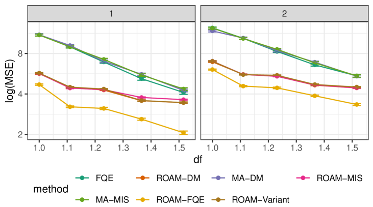
(a)

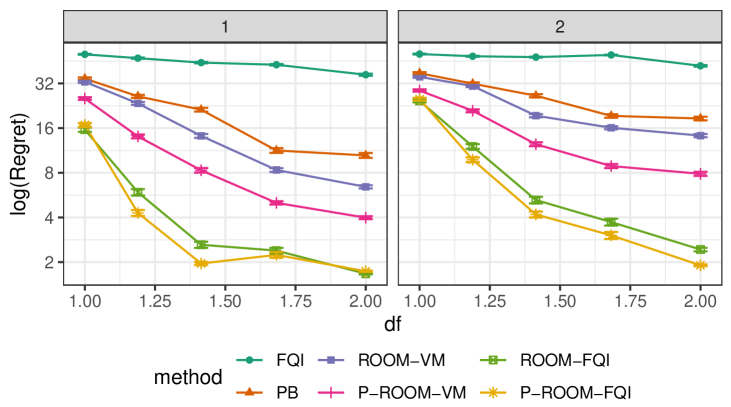
(b)

Figure 2: (a) OPE task: the trend of log(MSE) with the degree of freedom (df). (b) OPO task: The trend of regret with respect to the df. $\kappa$ takes value 1.0 (Left panel) and 2.0 (Right panel) in each subfigure. The error bar corresponds to 95% confidence interval.

Experiments: bootstrap-based ROAM

Since our proposal can be interpreted as ensembling multiple Q functions with a Median operator, another heuristic variant is using bootstrap instead of data partition. We conducted a comparison between this variant (denoted with the suffix “B-”) and ROAM-type methods, adopting the same settings as in the previous section. The results are visualized in Figure 3. It is evident that the vertical gap between ROAM-DM and B-ROAM-DM is negligible. Furthermore, they perform significantly better than the corresponding MA-type methods. This phenomenon also holds for MIS-type methods presented in the right panel. Therefore, we can conclude that bootstrap serves as an alternative implementation for the proposed procedure.

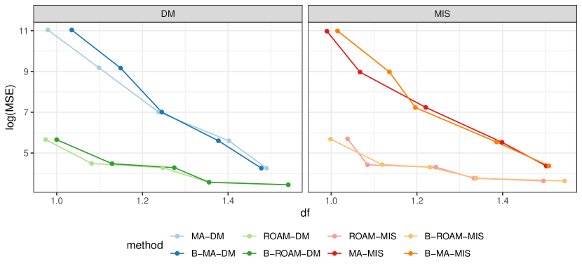
Figure 3: The left panel presents the results for DM methods, and the right one displays the results for MIS methods. To prevent point overlap, random noise has been added to each point on the $x$-axis.

Experiments for OPO (Cartpole environment). We study our algorithms:(i) ROOM-VM and (ii) ROOM-VM with pessimism (denoted as P-ROOM-VM), where BaseOPO are set as FQI. We compare two benchmark algorithms: FQI and the pessimistic-bootstrapping (PB) methods (Bai et al., 2022). See Appendix C.2.1 for detailed implementations. Motivated by the powerful performance of ROAM-FQE, we also consider employing MM (and its pessimism version) in the iteration of FQI. We name these algorithms ROOM-FQI and P-ROOM-FQI, and defer their definitions to Algorithm 5 in the Appendix. We generate 400 episodes to form an offline dataset following the same procedure described in experiments for OPE. To evaluate the performance of a learned policy $\hat{\pi}^{*}$, we compute its regret compared with the optimal policy.

We report the numerical results of 100 replications in Figure 2(b). We see that the regret of FQI reasonably decreases when df goes up, but it decreases more slowly when $\kappa$ enlarges. We can also observe that PB improves over FQI, because it can properly address the insufficient data coverage issue in OPO. However, due to the existence of heavy-tailed rewards, ROOM-VM and ROOM-FQI can outperform PB. Even though we have no theoretical guarantee for ROOM-FQI, it shows a better numerical performance compared with ROOM-VM. Finally, we turn to P-ROOM-VM and P-ROOM-FQI in Figure 2(b). As expected, P-ROOM-VM (or P-ROOM-FQI) performs better than ROOM-VM (or ROOM-FQI) because it addresses the insufficient data coverage issue and the heavy-tailedness simultaneously.

Experiments for OPO (D4RL datasets). We evaluate our proposed approach on the MuJoCo and Kitchen environments in the D4RL benchmarks (Fu et al., 2020), which cover diverse dataset settings and domains. We generate heavy-tailed datasets by adding i.i.d. noises into the reward observations, similar as the previous part. To show that the generality of our framework, in these datasets, we use another SOTA algorithm, sparsity Q-learning (SQL, Xu et al. (2023)), as our BaseOPO algorithm. For the sake of fairness, we also take into account the mean aggregation (denoted as MA). We train each algorithm for one million time steps and evaluate it every $5000$ time steps. Each evaluation consists of $10$ episodes. We show learning curves in Appendix.

We report the performance in Table 1. It is worth noting that, in all cases, our methods are superior to the vanilla SQL algorithm. The superiority can be highly significant. For example, on the halfcheetah-e dataset, ROOM-VM and P-ROOM-VM achieve a 30% improvement, and in the kitchen environment, our proposal shows a 200% improvement in SQL’s returns. This again shows that our proposal can effectively address the challenge of heavy-tailed rewards even in complex environments. The superiority of our proposal over MA reveals that the mean ensemble cannot handle heavy-tailed rewards but harm numerical performance because it has to use fewer samples to learn Q functions. Notably, in almost all cases, P-ROOM-VM surpasses ROOM-VM because P-ROOM-VM can more effectively address the issue of severe data insufficiency coverage. Furthermore, we also study the cases where BaseOPO is IQL (Kostrikov et al., 2022). The results reported in Appendix F.2 again show that our proposal has better performance than vanilla IQL, reflecting the versatility of our proposal. Finally, motivated by the success of the bootstrap-based variant and P-ROOM-FQI, we can further extend our proposal to the actor-critic paradigm and train agent with the whole dataset. Additionally, by setting $q=0.0$, this heuristic implementation leads to the exact SAC-N proposed by An et al. (2021), which is shown to be robust on heavy-tailed rewards in Figure A6 in the Appendix F.3.

	SQL	MA	ROOM-VM	P-ROOM-VM
halfcheetah-e	61.2$\pm$1.3	21.9$\pm$3.7	87.7$\pm$2.9	88.1$\pm$1.5
halfcheetah-m	39.8$\pm$0.6	30.7$\pm$0.4	41.7$\pm$0.2	42.1$\pm$0.2
halfcheetah-m-r	15.4$\pm$0.2	13.5$\pm$0.4	25.9$\pm$1.0	30.1$\pm$1.2
halfcheetah-f-l	32.3$\pm$0.9	26.5$\pm$0.6	49.4$\pm$1.0	52.5$\pm$0.8
walker2d-e	107.8$\pm$0.5	94.9$\pm$2.1	108.4$\pm$0.0	108.0$\pm$0.7
walker2d-m	59.3$\pm$0.6	25.8$\pm$2.1	69.9$\pm$2.3	64.0$\pm$3.5
walker2d-m-r	6.1$\pm$0.7	0.0$\pm$0.1	6.3$\pm$0.7	7.0$\pm$2.2
walker2d-f-l	7.2$\pm$1.5	2.8$\pm$0.4	14.7$\pm$3.0	22.3$\pm$3.5
hopper-e	33.4$\pm$2.5	1.7$\pm$0.0	17.5$\pm$0.3	35.1$\pm$4.2
hopper-m	14.5$\pm$0.5	6.6$\pm$0.0	38.5$\pm$0.5	31.8$\pm$2.3
hopper-m-r	3.3$\pm$0.0	2.1$\pm$0.0	10.6$\pm$0.5	6.3$\pm$0.1
hopper-f-l	1.4$\pm$0.0	1.9$\pm$0.0	3.1$\pm$0.2	9.7$\pm$0.8
kitchen-c	20.6$\pm$3.0	13.2$\pm$2.5	43.2$\pm$4.1	41.6$\pm$2.2
kitchen-p	8.7$\pm$1.9	6.4$\pm$1.7	26.5$\pm$1.8	33.8$\pm$1.9
kitchen-m	15.7$\pm$1.3	12.3$\pm$1.0	34.2$\pm$1.3	45.5$\pm$2.4

Table 1: Results on D4RL datasets. Note that -e=expert, -m=medium, -m-r=medium-replay, -f-r=full-replay, -c=complete, -p=-partial, -m=-mixed. Each result is the average normalized score that is taken over the final 10 evaluations and 5 seeds. $\pm$ captures the 2 times standard error over 5 seeds.

7 Conclusions

Motivated by the real needs for robust offline RL methods against heavy-tailed rewards, we leverage the MM method in robust statistics to design a new frameworks that can robustify existing OPE and OPO algorithms. Our methods are simple, general and naturally allow uncertainty quantification. Theoretical analysis demonstrates the advantages of our methods and extensive numerical studies support the empirical performance of our methods.

Appendix A Theoretical Proof

We use $c$ and $C$ to denote some general constants whose values are allowed to vary over time. Under Assumption 1, let $\{(S_{i},A_{i},R_{i},S_{i}^{\prime})\}_{i}$ denote the i.i.d. transition tuples.

A.1 Proof of Theorem 1

Proof.

Let $m=n/K$. The key to prove Theorem 1 is to show that for some properly chosen constant $c(\alpha)$ that depends only on $\alpha$ and

$$\Delta\geq c(\alpha)(\mathbb{E}|R|^{1+\alpha})^{\frac{1}{1+\alpha}}\Big{[}\|\widehat{\omega}^{\pi}-\omega^{\pi}\|_{\infty}+\|\omega^{\pi}\|_{\infty}\Big{(}\frac{1}{m}\Big{)}^{\frac{\alpha}{1+\alpha}}\Big{]},$$ (1)

then

$$\mathbb{P}\Big{(}\Big{|}\frac{1}{m}\sum_{i=1}^{m}\widehat{\omega}^{\pi}(S_{i},A_{i})R_{i}-\eta^{\pi}\Big{|}\geq\Delta\Big{)}\leq 0.2.$$ (2)

The rest of the proof can similarly be established based on the arguments in the proof of Theorem 1 of Lugosi and Mendelson (2019) and we omit the details to save space.

We focus on proving (2) below. We begin by considering the following decomposition,

$$\frac{1}{m}\sum_{i=1}^{m}\widehat{\omega}^{\pi}(S_{i},A_{i})R_{i}-\eta^{\pi}=\frac{1}{m}\sum_{i=1}^{m}\omega^{\pi}(S_{i},A_{i})R_{i}-\eta^{\pi}+\frac{1}{m}\sum_{i=1}^{m}[\widehat{\omega}^{\pi}(S_{i},A_{i})-\omega^{\pi}(S_{i},A_{i})]R_{i}.$$

For the first term, under Assumptions 2 and 3, the $(1+\alpha)$th moment of $\omega^{\pi}(S,A)R$ is upper bounded by $\|\omega^{\pi}\|_{\infty}{\mathbb{E}}|R|^{1+\alpha}$. Using the results in Bubeck et al. (2013) and Devroye et al. (2016), we can show that there exists some constant $c>0$ that depends only $\alpha$ such that

$$\mathbb{P}\Big{\{}\Big{|}\frac{1}{m}\sum_{i=1}^{m}\omega^{\pi}(S_{i},A_{i})R_{i}-\eta^{\pi}\Big{|}\geq c(\mathbb{E}|R|^{1+\alpha})^{\frac{1}{1+\alpha}}\|\omega^{\pi}\|_{\infty}\Big{(}\frac{1}{m}\Big{)}^{\frac{\alpha}{1+\alpha}}\Big{\}}\leq 0.1.$$ (3)

As for the second term, it is upper bounded by $\|\widehat{\omega}^{\pi}-\omega^{\pi}\|_{\infty}(m^{-1}\sum_{i=1}^{m}|R_{i}|)$. Consider $m^{-1}\sum_{i=1}^{m}|R_{i}|$. We decompose it into the sum of $m^{-1}\sum_{i=1}^{m}(|R_{i}|-\mathbb{E}|R|)$ and $\mathbb{E}|R|$. Similar to (3), we can show $m^{-1}\sum_{i=1}^{m}(|R_{i}|-\mathbb{E}|R|)$ satisfies the following,

$$\mathbb{P}\Big{\{}\Big{|}\frac{1}{m}\sum_{i=1}^{m}|R_{i}|-\mathbb{E}|R|\Big{|}\geq c(\mathbb{E}|R|^{1+\alpha})^{\frac{1}{1+\alpha}}\Big{(}\frac{1}{m}\Big{)}^{\frac{\alpha}{1+\alpha}}\Big{\}}\leq 0.1.$$ (4)

In addition, according to Hölder’s inequality, we have $\mathbb{E}|R|\leq(\mathbb{E}|R|^{1+\alpha})^{\frac{1}{1+\alpha}}$. This together with (4) implies that the second term can be upper bounded by $C\|\widehat{\omega}^{\pi}-\omega^{\pi}\|_{\infty}(\mathbb{E}|R|^{1+\alpha})^{\frac{1}{1+\alpha}}$ for some constant $C>0$, with probability at least $0.9$. Combining this together with (1) and (3) yields (2). ∎

A.2 Proof of Theorem 2

Proof.

Similar to the proof of Theorem 1, it suffices to show that each base OPE estimator satisfies (2) for any

$$\Delta\geq c(\alpha)\lambda_{\min}^{-1}(\mathbb{E}|R|^{1+\alpha})^{\frac{1}{1+\alpha}}\Big{(}\frac{1}{m}\Big{)}^{\frac{\alpha}{1+\alpha}}.$$

Under the realizability assumption and the boundedness assumption on $\phi$, the estimation error of the base OPE estimator is of the same order of magnitude as that of the based LSTD estimator $\widehat{\theta}$. It suffices to show that each base $\widehat{\theta}$ satisfies (2) for any

$$\Delta\geq c\lambda_{\min}^{-1}(\mathbb{E}|R|^{1+\alpha})^{\frac{1}{1+\alpha}}\Big{(}\frac{1}{m}\Big{)}^{\frac{\alpha}{1+\alpha}},$$

where $c$ denotes some positive constant that depends only on $\alpha$.

By definition, $\widehat{\theta}-\theta^{*}$ equals

$$\Big{[}\frac{1}{m}\sum_{i=1}^{m}\phi(S_{i},A_{i})\{\phi(S_{i},A_{i})-\gamma\sum_{a}\pi(a|S_{i}^{\prime})\phi(S_{i}^{\prime},a)\}^{\top}\Big{]}^{-1}$$

$$\times \Big{[}\frac{1}{m}\sum_{i=1}^{m}\phi(S_{i},A_{i})\{R_{i}+\gamma\sum_{a}\pi(a|S_{i}^{\prime})Q^{\pi}(S_{i}^{\prime},a)-Q^{\pi}(S_{i},A_{i})\}\Big{]}.$$

Under the matrix invertibility assumption, using similar arguments in the proof of Lemma 3 of Shi et al. (2022), we can show that the $\ell_{2}$ norm of the matrix

$$\Big{[}\frac{1}{m}\sum_{i=1}^{m}\phi(S_{i},A_{i})\{\phi(S_{i},A_{i})-\gamma\sum_{a}\pi(a|S_{i}^{\prime})\phi(S_{i}^{\prime},a)\}^{\top}\Big{]}^{-1}$$

can be upper bounded by $C\lambda_{\min}^{-1}$ with probability approaching $1$. As for the second term, using the results in Bubeck et al. (2013) and Devroye et al. (2016), we can show that its $\ell_{2}$ norm is upper bounded by $\mathbb{E}(|R|^{1+\alpha})^{\frac{1}{1+\alpha}}m^{-\frac{\alpha}{1+\alpha}}$ with probability at least $0.9$. Combining these results yield that

$$\mathbb{P}\Big{(}\|\widehat{\theta}-\theta^{*}\|_{2}\geq c(\mathbb{E}|R|^{1+\alpha})^{\frac{1}{1+\alpha}}\Big{(}\frac{1}{m}\Big{)}^{\frac{\alpha}{1+\alpha}}\Big{)}\leq 0.2,$$

for some constant $c>0$. The proof is hence completed. ∎

A.3 Proof of Theorem 3

Once Lemma 1 holds, we can follow a very similar proof for Theorem 2 to obtain the conclusion in Theorem 3. Thus, we only present the proof of Lemma 1.

Lemma 1.

Under the same notations and conditions in Lemma 2, then $\hat{\mu}^{\mathcal{Q}}_{q}$, the $q$-th quantile of $\{\hat{\mu}_{1},\ldots,\hat{\mu}_{K}\}$, satisfies

$$\mathbb{P}\left(\hat{\mu}-(12v)^{\frac{1}{1+\epsilon}}\left(\frac{1}{N}\right)^{\frac{\epsilon}{1+\epsilon}}>\hat{\mu}_{q}\right)\geq 1-\exp(-2K(2q-1)^{2}).$$

Proof.

According to Lemma 2, for each $l\in\{1,\ldots,K\}$, we have

$$\mathbb{P}\left(\mu-\eta\leq\hat{\mu}_{l}\right)\geq\mathbb{P}\left(|\hat{\mu}_{l}-\mu|\leq\eta\right)\geq 1-\frac{6v}{n^{\epsilon}\eta^{1+\epsilon}}.$$

Let $Y_{l}=I(\mu-\eta\leq\hat{\mu}_{l})$ with $p\coloneqq{\mathbb{E}}(Y_{l})\geq 1-\frac{6v}{n^{\epsilon}\eta^{1+\epsilon}}$. Then, according to the definition of $\hat{\mu}_{q}$, we have

$$\mathbb{P}\left(\mu-\eta\leq\hat{\mu}_{q}\right)=\mathbb{P}\left(\sum_{l=1}^{K}Y_{l}\geq qK\right)\leq\exp\left(-2K(q-p)^{2}\right),$$ (5)

where the second inequality comes from the Hoeffding inequality. Note that for

$$\eta=\left(\frac{6v}{q}\right)^{\frac{1}{1+\epsilon}}\left(\frac{1}{N}\right)^{\frac{\epsilon}{1+\epsilon}},$$

we can easily see that $p\geq 1-q\geq q$ (due to $q\leq 0.5$), and thus, Equation (5) can be simplified to:

$$\mathbb{P}\left(\mu-\eta\leq\hat{\mu}_{q}\right)\leq\exp\left(-2K(2q-1)^{2}\right).$$

∎

Lemma 2 (Bubeck et al. (2013)).

Let $\epsilon\in(0,1]$ and $X_{1},\ldots,X_{n}$ be i.i.d. random variable with mean $\mu$ and $(1+\epsilon)$-th moment ${\mathbb{E}}|X-\mu|^{1+\epsilon}=v$. Suppose each fold has $N$ observations such that $n=NK$, then for each $l\in\{1,\ldots,K\}$, the sample mean $\hat{\mu}_{l}=\frac{1}{N}\sum\limits_{t=(l-1)N+1}^{lN}X_{t}$ satisfies

$$\mathbb{P}\left(|\mu-\hat{\mu}_{l}|\geq\eta\right)\leq\frac{6v}{n^{\epsilon}\eta^{1+\epsilon}}$$

where for any $\eta>0$.

Appendix B Additional Algorithms

B.1 Important Sampling Variant

Algorithm 3 Robust Off-policy Evaluation via Median-of-means based Marginal Important Sampling (ROAM-MIS)

1:Policy $\pi$, data $\mathcal{D}$, number of data partitions $K$, decay rate $\gamma$, base marginal important sampling ratio estimation algorithm BaseMIS

2:Partition trajectories $\mathcal{D}$ into $K$ parts: $\mathcal{D}_{1},\ldots,\mathcal{D}_{K}$.

3:for $k=1,\dots,K$ do

4:     $\hat{\omega}^{\pi}_{k}\leftarrow\texttt{BaseMIS}(\pi,\mathcal{D}_{k},\gamma)$

5:end for

6:$\hat{\eta}^{\pi}\leftarrow\operatorname{Median}(\left\{\mathbb{E}_{\mathcal{D}_{k}}[\hat{\omega}^{\pi}_{k}(S,A)R]\right\}_{k=1}^{K})$

7:$\hat{\eta}^{\pi}$

B.2 The ROOM-FQE Algorithm

Algorithm 4 derives robust intermediate estimators by replacing the heavy-tailed target $Y=R+\gamma\mathbb{E}_{a\sim\pi(S^{\prime})}Q\left(S^{\prime},a\right)$ with a MM-type target $Y=R+\gamma\mathbb{E}_{a\sim\pi(S^{\prime})}\operatorname{Median}(\{\widehat{Q}^{\pi}_{k}\left(S^{\prime},a\right)\}_{k=1}^{K})$. However, one issue is that, these estimators $\{\widehat{Q}_{k}^{\pi}\}_{k=1}^{K}$ (and all estimators after this update including the final ones) in Algorithm 4 are not independent any longer. Therefore, it is not clear whether or not MM can still have theoretical benefits. Thus we only study this variant empirically.

Algorithm 4 Robust Off-policy Evaluation via Median-of-means based Fitted Q-Evaluation (ROAM-FQE)

1:Policy $\pi$, Data $\mathcal{D}$, decay rate $\gamma$, number of iterations $M$, number of partitions $K$.

2:Partition data $\mathcal{D}$ into $K$ disjoint parts: $\mathcal{D}_{1},\ldots,\mathcal{D}_{K}$

3:Initialize $K$ Q-functions $\widehat{Q}^{\pi}_{1},\ldots,\widehat{Q}^{\pi}_{K}$ with corresponding parameters $w_{1},\ldots,w_{K}$

4:for $m=1,\ldots,M$ do

5:     for $k=1,\ldots,K$ do

6:         For each $\left(S,A,R,S^{\prime}\right)\in\mathcal{D}_{k}$, compute: $Y\leftarrow R+\gamma\operatorname{Median}(\{\mathbb{E}_{a\sim\pi\left(S^{\prime}\right)}\widehat{Q}_{k}^{\pi}\left(S^{\prime},a\right)\}_{k=1}^{K})$

7:         Update $\widehat{Q}^{\pi}_{k}$ by: $w_{k}\leftarrow\underset{w_{k}}{\arg\min}\mathbb{E}_{\mathcal{D}_{k}}(Y-\widehat{Q}_{k}^{\pi}(S,A;w_{k}))^{2}$

8:     end for

9:end for

10:$\widehat{\eta}^{\pi}\leftarrow\mathbb{E}_{s\sim\mathbb{G},a\sim\pi(s)}\operatorname{Median}(\{\widehat{Q}_{k}^{\pi}(s,a)\}_{k=1}^{K})$

11:$\widehat{\eta}^{\pi}$

B.3 The ROOM-FQI Algorithm

Analogous to Algorithm 4, for iterative OPO algorithms, we can apply MM in every iteration. Take FQI as an example, we replace the definition of $Y$ in the Step 5 of Algorithm 4 by: $Y\leftarrow R+\gamma\operatorname{Median}(\{\max_{a}\widehat{Q}_{w_{k}}^{*}\left(S^{\prime},a\right)\}_{k=1}^{K})$, then we can obtain a robust FQI algorithm. Moreover, we also consider its pessimistic variant by using a quantile operator $\mathcal{Q}_{q}(\cdot)$ rather than the median operator in Step 5 of Algorithm 5. We denoted such a variant as P-ROOM-FQI.

Algorithm 5 Robust Offline-Policy Optimization via Median-of-mean based Fitted Q-Iteration (ROOM-FQI)

1:Data $\mathcal{D}$, decay rate $\gamma$, number of iterations $M$, number of data partitions $K$.

2:Partition data $\mathcal{D}$ into $K$ disjoint parts: $\mathcal{D}_{1},\ldots,\mathcal{D}_{K}$.

3:Initialize Q-functions $\widehat{Q}^{*}_{1},\ldots,\widehat{Q}^{*}_{K}$ with parameters $w_{1},\ldots,w_{K}$.

4:for $m=1,\dots,M$ do

5:     for $k=1,\dots,K$ do

6:         For each $\left(S,A,R,S^{\prime}\right)\in\mathcal{D}_{k}$, compute: $Y=R+\gamma\max\limits_{a}\operatorname{Median}(\{\widehat{Q}^{*}_{k}(S^{\prime},a)\}_{k=1}^{K})$.

7:         Update $Q_{k}$: $w_{k}\leftarrow\arg\min_{w_{k}}\mathbb{E}_{\mathcal{D}_{k}}(Y-\widehat{Q}^{*}_{k}(S,A;w_{k}))^{2}$.

8:     end for

9:end for

10:$\hat{\pi}^{*}(s)\leftarrow\operatorname*{arg\;\!max}\limits_{a}\textup{Median}(\{Q_{k}(s,a)\}_{k=1}^{K})$.

11:Policy $\hat{\pi}^{*}$

Appendix C Implementation Details

C.1 Settings for OPE

In the experiments for OPE (see Section 6), we implement the minimax-optimal off-policy evaluation algorithm (Duan et al., 2020) as the benchmarke FQI algorithm. Specifically, we use Ridge in scikit-learn with $\ell_{2}$-penalty fixed at 0.01. The implemented FQI algorithm serves as the BaseOPE algorithm for ROAM-DM. The implementation of ROAM-FQE also uses the same Ridge to update $Q_{w_{k}}$ in the Step 6 in Algorithm 4. The maximum number of iterations of all algorithms in Section 6 are fixed at 100.

Next, we discuss the tuning of our algorithms. The only additional tuning parameter of ROAM-type algorithms is the number of partitions $K$, compared with its corresponding base algorithm. In our experiments, fixing $K=5$ already provides the desired performance and maintains a high computational efficiency. In Appendix F.4, we try a range of values for $K$ and find that our algorithms are insensitive to this tuning parameter. One may choose this parameter via an adaptive method (Lugosi and Mendelson, 2019) as well.

C.2 Settings for OPO

C.2.1 Cartpole environment

For the experiments for OPO at Section 6, we implement the ridge-regression-based FQI algorithm as the benchmarked algorithm and the BaseOPO algorithm for ROOM-VM. The FQI uses Ridge in scikit-learn to solve the optimal Q-function. Here, we set the $\ell_{2}$-penalty of Ridge as 20 to stablize the computation. We implement the ROOM-FQI with the same ridge regression with the same settings. For pessimistic variant of ROOM-type algorithms, we need an additional tuning parameter $q$, i.e., the quantile level. As argued in Zhou et al. (2022), the fact that one quantile explicitly corresponds to one confidence level makes the tuning much easier than most existing methods where the relationship between the pessimism parameters and the confidence level is implicit and unknown. According to empirical results in Appendix F.5, we find $q\in[0.1,0.4]$ perform fairly well. We fix $q=0.1$ in our experiments.

We also implement a pessimistic-bootstapping OPO method, PB, to give a more comprehensive comparison. It is the same as ROOM-VM except the two modifications:

• the Step 1 in Algorithm 2 is changed to: “Sample $K$ bootstrapped samples from $\mathcal{D}$: $\mathcal{D}_{1},\ldots,\mathcal{D}_{K}$”;

• the Step 5 in Algorithm 2 is modified to:

  $$\hat{\pi}(s)\leftarrow\arg\max\limits_{a}\left[\textup{Mean}(\{\hat{Q}_{k}(s,a)\}_{k=1}^{K})-2\times\textup{Std}(\{\hat{Q}_{k}(s,a)\}_{k=1}^{K})\right]\;\textup{for any}\;s.$$

C.2.2 Mujoco environments

Datasets. All D4RL datasets (Fu et al., 2020) on MuJoCo environments in the experiments are the “v2” version. The datasets on the Kitchen environment are the “v0” version.

Network architecture. The implementations of SQL is based on an open-source implementations from GitHub, which largely reproduce the results in Kostrikov et al. (2022). Following the same architecture in SQL, both the critic and value networks are two-layer multi-layer perceptron (MLP) with 256 hidden nodes and ReLU activations. We recruit a deterministic policy network whose architecture is the same as critic network.

The implementation of N-SAC is upon a public Github repository for SAC. Our implementation completely adopt the same actor-critic architecture in An et al. (2021). Specifically, the critic network is a three-layer MLPs with 256 hidden nodes and ReLU activations. The policy in SAC-N is a Gaussian policy network which enables automatic entropy tuning. As for SAC-N (STD) to be introduced in Section F.3, it inherits the same architecture and hyperparameters as SAC-N.

Hyperparameters. For the behavior-regularized term $\alpha$ in SQL, we set $\alpha=10$ since Table 3 in Xu et al. (2023) reports $\alpha=10$ leads to the best average result in MuJoCo environment. For the remaining parameter in SQL, we use default hyperparameters according to the GitHub, which are listed in Table A2. Notice that, once we complete training ROOM-VM, the learned critics can be reused for MA and P-ROOM-VM. We recruit this trick to reduce the experiments.

	Hyperparameter	Value
SQL	Optimizer	Adam (Kingma and Ba, 2014)
	Value/Critic learning rate	$3^{-4}$
	Actor learning rate	Cosine schedule (Loshchilov and Hutter, 2017)
	Critic target update rate	$5\times 10^{-3}$
	Mini-batch size	256
	behavior-regularized $\alpha$	10
ROOM-VM & MA	Data partition $K$	5
P-ROOM-VM	Quantile $q$	0.0

Table A2: The hyperparameters of SQL used in the experiments for D4RL tasks.

We summarized the hyperparameters for train SAC-N in Table A3.

Hyperparameter	Value
Critic/actor learning rate	$3^{-4}$
Critic target update rate	$5\times 10^{-3}$
Mini-batch size	256
Ensemble number (a.k.a., $K$)	10
Temperature	0.2

Table A3: The hyperparameters of SAC-N used in the experiments for D4RL tasks.

Appendix D Computation Details: Cost and Infrastructure

Let the computational cost of the base algorithm be $c(N)$ for a dataset with $N$ transition tuples. Our algorithm in general yields $\mathcal{O}(K\times c(N/K))$. For those based methods that have a linear computational cost in $N$ (e.g., FQE and FQI; see derivations in Shi et al. (2021)), our computational cost is at the same order. Moreover, our method is embarrassingly parallel.

The experiments in Carpole environment will finish in 5 hours on a personal laptop with 2.6 GHz 6-Core Intel Core i7 and 16 GB memory.

As for the experiments for D4RL datasets, ROOM-VM generally consumes 14 hours to train a agent on a task with a machine with GPU Tesla P-100, while SAC-N roughly takes round 30 hours to train on the same device.

Appendix E Broader Impact and Future directions

Our approach provides offline RL methods to be applied to systems with heavy-tailed rewards. While our method can properly handle heavy-tailed rewards, it may also neglect the potential societal impact. For instance, heavy-tailed rewards in finance system may arise from fraudulent transactions or attacks on banking systems, which deserves adequate attention. One possible approach to monitor heavy-tailed rewards involves measures the gap between the two sides of Bellman equation. If the resulting value exhibits high variance, then the rewards warrants monitoring.

One limitation of ROOM is that it requires maintaining $K$ models in memory when deploying the policy. To address the concern, one can first train $\widehat{Q}^{*}=\arg\min_{Q}\mathbb{E}_{\mathcal{D}}(Q(S,A)-\operatorname{Median}(\{\widehat{Q}^{*}_{k}(S,A)\}_{k=1}^{K}))^{2}$ and then output the policy $\hat{\pi}^{*}(s)\coloneqq\arg\max_{a}\widehat{Q}^{*}(s,a)$. Additionally, it would be intriguing to extend our approach by formulating a generalized Bellman equation to address scenarios where the mean of rewards is non-existent.

Appendix F Additional Experiments

F.1 Learning curves of SQL

Figures A4 and A5 present the learning curves on MuJoCo and Kitchen environments, where the evaluations is conducted every 5000 training steps. Each curve is averaged over 5 seeds and is smoothed by simple moving averages over three periods.

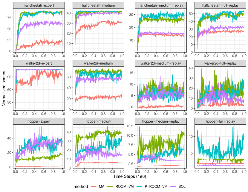
Figure A4: Learning curves of SQL, MA, ROOM-VM, P-ROOM-VM on D4RL MuJoCo locomotion datasets.

Figure A5: Learning curves of SQL, MA, ROOM-VM, P-ROOM-VM on D4RL Kitchen datasets.

F.2 Comparison with IQL

To show that our framework is general, in these datasets, we use another SOTA algorithm, implicit Q-learning (IQL, Kostrikov et al. (2022)), as our BaseOPO algorithm. We run IQL using the open-source implementation. Notably, the simplicity of ROOM-VM requires minimal modifications of the existing implementation. We adopt the data generation and model evaluation in Section 6.

We report the performance in Table A4. In almost all cases, our method is significantly superior to IQL. Notably, ROOM-VM can tackle the insufficient coverage challenge by employing IQL that can cope with insufficient coverage (Xu et al., 2023). Moreover, the superiority of ROOM-VM and P-ROOM-VM are clearer in the walker and hopper environments, because these two environments are more challenging than others. For example, the returns of ROOM-VM and P-ROOM-VM on walker-medium are 20% higher than that of IQL, and the returns of ROOM-VM and P-ROOM-VM on hopper-expert are about 200% of IQL’s returns. It is also worth noting that P-ROOM-VM shows comparable performance with ROOM-VM in most cases, and P-ROOM-VM has superior performance in the expert generating datasets because this setup has more severe data insufficient coverage issue.

Task Name	ROOM-VM	P-ROOM-VM
halfcheetah-expert	1.04 $\pm$ 0.02	1.03 $\pm$ 0.02
walker2d-expert	1.02 $\pm$ 0.02	1.02 $\pm$ 0.02
hopper-expert	1.89 $\pm$ 0.12	2.14 $\pm$ 0.13
halfcheetah-medium	0.99 $\pm$ 0.01	0.98 $\pm$ 0.01
walker2d-medium	1.31 $\pm$ 0.08	1.40 $\pm$ 0.06
hopper-medium	1.32 $\pm$ 0.03	1.28 $\pm$ 0.02
halfcheetah-medium-replay	1.04 $\pm$ 0.04	1.02 $\pm$ 0.05
walker2d-medium-replay	1.56 $\pm$ 0.26	0.95 $\pm$ 0.16
hopper-medium-replay	1.15 $\pm$ 0.14	1.20 $\pm$ 0.11

Table A4: Results for D4RL datasets. Each result is the division of average normalized score of ROOM-VM (or P-ROOM-VM) and IQL. We takes over the final 10 evaluations and 5 seeds. $\pm$ captures the 2 times standard error over 5 seeds.

F.3 Robustness of SAC-N

It’s noteworthy that SAC-N (An et al., 2021) can be interpret to P-ROOM-FQI, as it assesses uncertainty by taking the pointwise minimum (i.e., setting $q=0.0$) of multiple Q-functions but trained on the entire dataset with an soft-actor-critic (SAC) paradigm. Hence, we can be regarded as a heuristic implementation of our approach, and we can expect that it enjoys robustness on heavy-tailed rewards.

To illustrate, we implement SAC-N and compare with SAC-N (STD), a method that achieves pessimistic estimation for Q function by pointwisely subtracting two times standard deviation of $N$ functions. To rephrase, SAC-N (STD) replaces the pointwise quantile $\mathcal{Q}_{q}(\{Q_{k}(s,a)\}_{k=1}^{N})$ with $\textup{Mean}(\{Q_{k}(s,a)\}_{k=1}^{N})-2\times\textup{Std}(\{Q_{k}(s,a)\}_{k=1}^{N})$. We demonstrate the numerical performance SAC-N and SAC-N (STD) on halfcheetah-medium-v2 in Figure A6. From the left panel of Figure A6, we can see that the results of SAC-N are highly resembles to the results of Figure 1 in An et al. (2021). More importantly, despite SAC-N and SAC-N (STD) shares almost the same learning behavior when datasets has no heavy-tailed rewards (see left panel of Figure A6), we can see that SAC-N is shown to be much robust to the heavy-tailed noises while SAC-N (STD) completely fails at this case. Therefore, it is also highly recommended to use SAC-N in environments with heavy-tailed rewards.

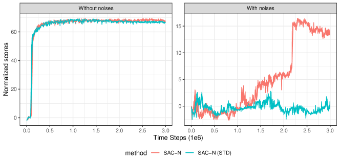
Figure A6: Learning curves comparing the performance of SAC-N against SAC-N-STD on the halfcheetah-medium-v2 dataset where the left panel corresponds to the case that heavy-tailed noises are not taken into consideration and the right one vice versa. Curves are averaged over 5 seeds and are smoothed by simple moving averages over three periods.

F.4 Selection of $K$

In this part, we aim to study how the selection of $K$ influence the performance of ROAM-DM. Out of simplicity, we consider values for $K\in\{3,4,\ldots,10\}$, while the other settings adopt that in Section 6. The estimation error of each algorithm is visualized in Figure A7. From Figure A7, we can see that, our methods exceeds FQE for all $K\in\{3,4,\ldots,10\}$. This implies that, whatever $K$ is taken, our methods are more suitable than FQE for offline data with heavy-tailed rewards. It is also worthy to note that, the optimal value of $K$ varies across algorithms and the degree of freedom of the heavy-tailed rewards. In terms of degree of freedom, since it is unknown in practice, there has no general criteria to decide the optimal $K$. We suggest $K=5$ as a rule-of-thumb selection for all of our methods because this selection can result in a good performance. Notice that the comparison between ROAM-based methods and mean aggregation methods reveals taking the median operator is crucial for robustness — the mean aggregation achieves a poor performance.

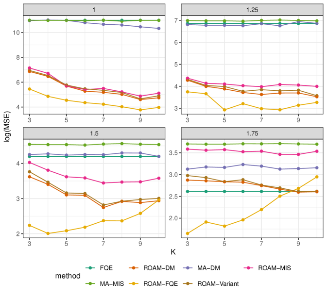
Figure A7: The Ablation on the tuning parameter $K$ for the OPE problem at the Cartpole environment. Each panel corresponds to a certain degree of freedom.

F.5 Selection of Pessimistic

In this part, we aim to study how the selection of $q$ influence the performance of ROAM-DM and ROOM-FQI. We consider values for $q\in\{0.1,0.2,0.3,0.4,0.5\}$, while the other settings adopt that in the experiments on Cartpole environment. We visualize the regret of each algorithm in Figure A7, from which we see that, our methods surpass FQI whatever the value of $q$. Besides, like the choice for $K$, both algorithms and the degree of freedom of the heavy-tailed rewards have an impact on the optimal value of $q$. Figure A8 shows $q\in[0.1,0.4]$ is a rule-of-thumb criterion for the guarantee of admirable numerical performance.

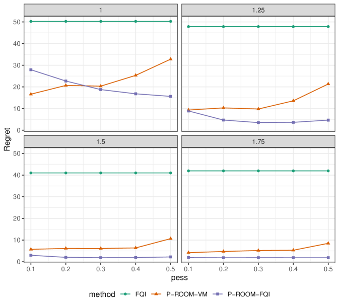
Figure A8: The ablation on the tuning parameter $q$ for the OPE problem at the Cartpole environment. Each panel corresponds to a certain degree of freedom.

References

- Alon et al. (1996) Alon, N., Y. Matias, and M. Szegedy (1996). The space complexity of approximating the frequency moments. In Proceedings of the twenty-eighth annual ACM symposium on Theory of computing, pp. 20–29.
- An et al. (2021) An, G., S. Moon, J.-H. Kim, and H. O. Song (2021). Uncertainty-based offline reinforcement learning with diversified q-ensemble. Advances in neural information processing systems 34, 7436–7447.
- Bai et al. (2022) Bai, C., L. Wang, Z. Yang, Z.-H. Deng, A. Garg, P. Liu, and Z. Wang (2022). Pessimistic bootstrapping for uncertainty-driven offline reinforcement learning. In International Conference on Learning Representations.
- Bertsekas (2012) Bertsekas, D. (2012). Dynamic programming and optimal control: Volume I, Volume 1. Athena scientific.
- Bhandari et al. (2021) Bhandari, J., D. Russo, and R. Singal (2021). A finite time analysis of temporal difference learning with linear function approximation. Operations Research 69(3), 950–973.
- Boyan (1999) Boyan, J. A. (1999). Least-squares temporal difference learning. In ICML, pp. 49–56.
- Bradtke and Barto (1996) Bradtke, S. J. and A. G. Barto (1996). Linear least-squares algorithms for temporal difference learning. Machine learning 22(1), 33–57.
- Brandfonbrener et al. (2021) Brandfonbrener, D., W. Whitney, R. Ranganath, and J. Bruna (2021). Offline rl without off-policy evaluation. Advances in Neural Information Processing Systems 34, 4933–4946.
- Bubeck et al. (2013) Bubeck, S., N. Cesa-Bianchi, and G. Lugosi (2013). Bandits with heavy tail. IEEE Transactions on Information Theory 59(11), 7711–7717.
- Chen and Jiang (2019) Chen, J. and N. Jiang (2019). Information-theoretic considerations in batch reinforcement learning. In International Conference on Machine Learning, pp. 1042–1051. PMLR.
- Chen and Qi (2022) Chen, X. and Z. Qi (2022). On well-posedness and minimax optimal rates of nonparametric q-function estimation in off-policy evaluation. In International Conference on Machine Learning, pp. 3558–3582. PMLR.
- Chen et al. (2021) Chen, Y., S. Du, and K. Jamieson (2021). Improved corruption robust algorithms for episodic reinforcement learning. In International Conference on Machine Learning, pp. 1561–1570. PMLR.
- Dadashi et al. (2021) Dadashi, R., S. Rezaeifar, N. Vieillard, L. Hussenot, O. Pietquin, and M. Geist (2021). Offline reinforcement learning with pseudometric learning. In International Conference on Machine Learning, pp. 2307–2318. PMLR.
- Dai et al. (2020) Dai, B., O. Nachum, Y. Chow, L. Li, C. Szepesvari, and D. Schuurmans (2020). Coindice: Off-policy confidence interval estimation. Advances in neural information processing systems 33.
- Devroye et al. (2016) Devroye, L., M. Lerasle, G. Lugosi, and R. I. Oliveira (2016). Sub-gaussian mean estimators. The Annals of Statistics 44(6), 2695–2725.
- Duan et al. (2020) Duan, Y., Z. Jia, and M. Wang (2020). Minimax-optimal off-policy evaluation with linear function approximation. In International Conference on Machine Learning, pp. 2701–2709. PMLR.
- Ernst et al. (2005) Ernst, D., P. Geurts, and L. Wehenkel (2005). Tree-based batch mode reinforcement learning. Journal of Machine Learning Research 6.
- Fan et al. (2020) Fan, J., Z. Wang, Y. Xie, and Z. Yang (2020). A theoretical analysis of deep q-learning. In Learning for Dynamics and Control, pp. 486–489. PMLR.
- Farajtabar et al. (2018) Farajtabar, M., Y. Chow, and M. Ghavamzadeh (2018). More robust doubly robust off-policy evaluation. In International Conference on Machine Learning, pp. 1447–1456. PMLR.
- Fu et al. (2020) Fu, J., A. Kumar, O. Nachum, G. Tucker, and S. Levine (2020). D4rl: Datasets for deep data-driven reinforcement learning. arXiv preprint arXiv:2004.07219.
- Fu et al. (2022) Fu, Y., D. Wu, and B. Boulet (2022). A closer look at offline rl agents. Advances in Neural Information Processing Systems 35, 8591–8604.
- Fu et al. (2022) Fu, Z., Z. Qi, Z. Wang, Z. Yang, Y. Xu, and M. R. Kosorok (2022). Offline reinforcement learning with instrumental variables in confounded markov decision processes. arXiv preprint arXiv:2209.08666.
- Fujimoto and Gu (2021) Fujimoto, S. and S. S. Gu (2021). A minimalist approach to offline reinforcement learning. Advances in neural information processing systems 34, 20132–20145.
- Georgiou et al. (1999) Georgiou, P. G., P. Tsakalides, and C. Kyriakakis (1999). Alpha-stable modeling of noise and robust time-delay estimation in the presence of impulsive noise. IEEE transactions on multimedia 1(3), 291–301.
- Gerstenberg et al. (2022) Gerstenberg, J., R. Neininger, and D. Spiegel (2022). On solutions of the distributional bellman equation. arXiv preprint arXiv:2202.00081.
- Goyal and Grand-Clement (2023) Goyal, V. and J. Grand-Clement (2023). Robust markov decision processes: Beyond rectangularity. Mathematics of Operations Research 48(1), 203–226.
- Guo et al. (2022) Guo, K., Y. Shao, and Y. Geng (2022). Model-based offline reinforcement learning with pessimism-modulated dynamics belief. NeurIPS.
- Hall (1990) Hall, P. (1990). Asymptotic properties of the bootstrap for heavy-tailed distributions. The Annals of Probability, 1342–1360.
- Hamza and Krim (2001) Hamza, A. B. and H. Krim (2001). Image denoising: A nonlinear robust statistical approach. IEEE transactions on signal processing 49(12), 3045–3054.
- Hanna et al. (2019) Hanna, J., S. Niekum, and P. Stone (2019, 09–15 Jun). Importance sampling policy evaluation with an estimated behavior policy. In K. Chaudhuri and R. Salakhutdinov (Eds.), Proceedings of the 36th International Conference on Machine Learning, Volume 97 of Proceedings of Machine Learning Research, pp. 2605–2613. PMLR.
- Huang and Zhang (2017) Huang, Y. and Y. Zhang (2017). A new process uncertainty robust student’st based kalman filter for sins/gps integration. IEEE Access 5, 14391–14404.
- Jiang and Huang (2020) Jiang, N. and J. Huang (2020). Minimax value interval for off-policy evaluation and policy optimization. Advances in Neural Information Processing Systems 33, 2747–2758.
- Jiang and Li (2016) Jiang, N. and L. Li (2016). Doubly robust off-policy value evaluation for reinforcement learning. In International Conference on Machine Learning, pp. 652–661. PMLR.
- Jin et al. (2021) Jin, Y., Z. Yang, and Z. Wang (2021). Is pessimism provably efficient for offline rl? In International Conference on Machine Learning, pp. 5084–5096. PMLR.
- Kallus et al. (2022) Kallus, N., X. Mao, K. Wang, and Z. Zhou (2022). Doubly robust distributionally robust off-policy evaluation and learning. pp. 10598–10632.
- Kallus and Uehara (2020) Kallus, N. and M. Uehara (2020). Double reinforcement learning for efficient off-policy evaluation in markov decision processes. Journal of Machine Learning Research 21(167).
- Kallus and Uehara (2022) Kallus, N. and M. Uehara (2022). Efficiently breaking the curse of horizon in off-policy evaluation with double reinforcement learning. Operations Research.
- Kingma and Ba (2014) Kingma, D. P. and J. Ba (2014). Adam: A method for stochastic optimization.
- Kostrikov et al. (2021) Kostrikov, I., R. Fergus, J. Tompson, and O. Nachum (2021). Offline reinforcement learning with fisher divergence critic regularization. In International Conference on Machine Learning, pp. 5774–5783. PMLR.
- Kostrikov et al. (2022) Kostrikov, I., A. Nair, and S. Levine (2022). Offline reinforcement learning with implicit q-learning. In International Conference on Learning Representations.
- Kumar et al. (2019) Kumar, A., J. Fu, M. Soh, G. Tucker, and S. Levine (2019). Stabilizing off-policy q-learning via bootstrapping error reduction. Advances in Neural Information Processing Systems 32.
- Kumar et al. (2020) Kumar, A., A. Zhou, G. Tucker, and S. Levine (2020). Conservative q-learning for offline reinforcement learning. Advances in Neural Information Processing Systems 33, 1179–1191.
- Lagoudakis and Parr (2003) Lagoudakis, M. G. and R. Parr (2003). Least-squares policy iteration. Journal of Machine Learning Research 4, 1107–1149.
- Le et al. (2019) Le, H., C. Voloshin, and Y. Yue (2019). Batch policy learning under constraints. In International Conference on Machine Learning, pp. 3703–3712. PMLR.
- Levine et al. (2020) Levine, S., A. Kumar, G. Tucker, and J. Fu (2020). Offline reinforcement learning: Tutorial, review, and perspectives on open problems. arXiv preprint arXiv:2005.01643.
- Liao et al. (2021) Liao, P., P. Klasnja, and S. Murphy (2021). Off-policy estimation of long-term average outcomes with applications to mobile health. Journal of the American Statistical Association 116(533), 382–391.
- Liao et al. (2022) Liao, P., Z. Qi, R. Wan, P. Klasnja, and S. A. Murphy (2022). Batch policy learning in average reward markov decision processes. The Annals of Statistics 50(6), 3364–3387.
- Liu et al. (2018) Liu, Q., L. Li, Z. Tang, and D. Zhou (2018). Breaking the curse of horizon: Infinite-horizon off-policy estimation. Advances in Neural Information Processing Systems 31.
- Loshchilov and Hutter (2017) Loshchilov, I. and F. Hutter (2017). SGDR: Stochastic gradient descent with warm restarts. In International Conference on Learning Representations.
- Lu et al. (2019) Lu, S., G. Wang, Y. Hu, and L. Zhang (2019). Optimal algorithms for lipschitz bandits with heavy-tailed rewards. In International Conference on Machine Learning, pp. 4154–4163. PMLR.
- Luckett et al. (2020) Luckett, D. J., E. B. Laber, A. R. Kahkoska, D. M. Maahs, E. Mayer-Davis, and M. R. Kosorok (2020). Estimating dynamic treatment regimes in mobile health using v-learning. Journal of the American Statistical Association 115(530), 692–706.
- Lugosi and Mendelson (2019) Lugosi, G. and S. Mendelson (2019). Mean estimation and regression under heavy-tailed distributions: A survey. Foundations of Computational Mathematics 19(5), 1145–1190.
- Lykouris et al. (2021) Lykouris, T., M. Simchowitz, A. Slivkins, and W. Sun (2021). Corruption-robust exploration in episodic reinforcement learning. In Conference on Learning Theory, pp. 3242–3245. PMLR.
- Lyu et al. (2022) Lyu, J., X. Ma, X. Li, and Z. Lu (2022). Mildly conservative q-learning for offline reinforcement learning. In A. H. Oh, A. Agarwal, D. Belgrave, and K. Cho (Eds.), Advances in Neural Information Processing Systems.
- Mannor et al. (2016) Mannor, S., O. Mebel, and H. Xu (2016). Robust mdps with k-rectangular uncertainty. Mathematics of Operations Research 41(4), 1484–1509.
- Min et al. (2021) Min, Y., T. Wang, D. Zhou, and Q. Gu (2021). Variance-aware off-policy evaluation with linear function approximation. Advances in neural information processing systems 34, 7598–7610.
- Minsker (2015) Minsker, S. (2015). Geometric median and robust estimation in banach spaces. Bernoulli 21(4), 2308–2335.
- Mo et al. (2021) Mo, W., Z. Qi, and Y. Liu (2021). Learning optimal distributionally robust individualized treatment rules. Journal of the American Statistical Association 116(534), 659–674.
- Munos and Szepesvári (2008) Munos, R. and C. Szepesvári (2008). Finite-time bounds for fitted value iteration. Journal of Machine Learning Research 9(5).
- Nachum et al. (2019) Nachum, O., Y. Chow, B. Dai, and L. Li (2019). Dualdice: Behavior-agnostic estimation of discounted stationary distribution corrections. Advances in Neural Information Processing Systems 32.
- Nemirovskij and Yudin (1983) Nemirovskij, A. S. and D. B. Yudin (1983). Problem complexity and method efficiency in optimization.
- Nilim and El Ghaoui (2005) Nilim, A. and L. El Ghaoui (2005). Robust control of markov decision processes with uncertain transition matrices. Operations Research 53(5), 780–798.
- Pedregosa et al. (2011) Pedregosa, F., G. Varoquaux, A. Gramfort, V. Michel, B. Thirion, O. Grisel, M. Blondel, P. Prettenhofer, R. Weiss, V. Dubourg, et al. (2011). Scikit-learn: Machine learning in python. Journal of Machine Learning Research 12, 2825–2830.
- Perdomo et al. (2022) Perdomo, J. C., A. Krishnamurthy, P. Bartlett, and S. Kakade (2022). A sharp characterization of linear estimators for offline policy evaluation. arXiv preprint arXiv:2203.04236.
- Precup (2000) Precup, D. (2000). Eligibility traces for off-policy policy evaluation. Computer Science Department Faculty Publication Series, 80.
- Prudencio et al. (2023) Prudencio, R. F., M. R. O. A. Maximo, and E. L. Colombini (2023). A survey on offline reinforcement learning: Taxonomy, review, and open problems. IEEE Transactions on Neural Networks and Learning Systems, 1–0.
- Ruotsalainen et al. (2018) Ruotsalainen, L., M. Kirkko-Jaakkola, J. Rantanen, and M. Mäkelä (2018). Error modelling for multi-sensor measurements in infrastructure-free indoor navigation. Sensors 18(2), 590.
- Schulman et al. (2017) Schulman, J., F. Wolski, P. Dhariwal, A. Radford, and O. Klimov (2017). Proximal policy optimization algorithms. arXiv preprint arXiv:1707.06347.
- Shao et al. (2018) Shao, H., X. Yu, I. King, and M. R. Lyu (2018). Almost optimal algorithms for linear stochastic bandits with heavy-tailed payoffs. Advances in Neural Information Processing Systems 31.
- Shi et al. (2021) Shi, C., R. Wan, V. Chernozhukov, and R. Song (2021). Deeply-debiased off-policy interval estimation. In International Conference on Machine Learning, pp. 9580–9591. PMLR.
- Shi et al. (2022) Shi, C., S. Zhang, W. Lu, and R. Song (2022). Statistical inference of the value function for reinforcement learning in infinite-horizon settings. Journal of the Royal Statistical Society: Series B (Statistical Methodology) 84(3), 765–793.
- Shi et al. (2022) Shi, L., G. Li, Y. Wei, Y. Chen, and Y. Chi (2022). Pessimistic q-learning for offline reinforcement learning: Towards optimal sample complexity. International Conference on Machine Learning.
- Si et al. (2020) Si, N., F. Zhang, Z. Zhou, and J. Blanchet (2020). Distributionally robust policy evaluation and learning in offline contextual bandits. In International Conference on Machine Learning, pp. 8884–8894. PMLR.
- Sutton and Barto (2018) Sutton, R. S. and A. G. Barto (2018). Reinforcement learning: An introduction. MIT press.
- Sutton et al. (2008) Sutton, R. S., C. Szepesvári, and H. R. Maei (2008). A convergent o(n) algorithm for off-policy temporal-difference learning with linear function approximation. Advances in neural information processing systems 21(21), 1609–1616.
- Tang et al. (2019) Tang, Z., Y. Feng, L. Li, D. Zhou, and Q. Liu (2019). Doubly robust bias reduction in infinite horizon off-policy estimation. arXiv preprint arXiv:1910.07186.
- Thomas and Brunskill (2016) Thomas, P. and E. Brunskill (2016). Data-efficient off-policy policy evaluation for reinforcement learning. In International Conference on Machine Learning, pp. 2139–2148. PMLR.
- Thomas et al. (2015) Thomas, P., G. Theocharous, and M. Ghavamzadeh (2015). High-confidence off-policy evaluation. In Proceedings of the AAAI Conference on Artificial Intelligence, Volume 29.
- Uehara et al. (2020) Uehara, M., J. Huang, and N. Jiang (2020). Minimax weight and q-function learning for off-policy evaluation. In International Conference on Machine Learning, pp. 9659–9668. PMLR.
- Uehara et al. (2022) Uehara, M., C. Shi, and N. Kallus (2022). A review of off-policy evaluation in reinforcement learning. arXiv preprint arXiv:2212.06355.
- Uehara and Sun (2022) Uehara, M. and W. Sun (2022). Pessimistic model-based offline reinforcement learning under partial coverage. In International Conference on Learning Representations.
- Voloshin et al. (2021) Voloshin, C., H. M. Le, N. Jiang, and Y. Yue (2021). Empirical study of off-policy policy evaluation for reinforcement learning. In Thirty-fifth Conference on Neural Information Processing Systems Datasets and Benchmarks Track (Round 1).
- Wang et al. (2022) Wang, J., R. Gao, and H. Zha (2022). Reliable off-policy evaluation for reinforcement learning. Operations Research.
- Wang et al. (2021) Wang, J., Z. Qi, and R. K. Wong (2021). Projected state-action balancing weights for offline reinforcement learning. arXiv preprint arXiv:2109.04640.
- Wang et al. (2018) Wang, Q., J. Xiong, L. Han, H. Liu, T. Zhang, et al. (2018). Exponentially weighted imitation learning for batched historical data. Advances in Neural Information Processing Systems 31.
- Wang et al. (2021) Wang, R., Y. Wu, R. Salakhutdinov, and S. Kakade (2021). Instabilities of offline rl with pre-trained neural representation. In International Conference on Machine Learning, pp. 10948–10960. PMLR.
- Wiesemann et al. (2013) Wiesemann, W., D. Kuhn, and B. Rustem (2013). Robust markov decision processes. Mathematics of Operations Research 38(1), 153–183.
- Wu et al. (2020) Wu, Y., G. Tucker, and O. Nachum (2020). Behavior regularized offline reinforcement learning.
- Xie et al. (2021) Xie, T., C.-A. Cheng, N. Jiang, P. Mineiro, and A. Agarwal (2021). Bellman-consistent pessimism for offline reinforcement learning. Advances in neural information processing systems 34, 6683–6694.
- Xie et al. (2019) Xie, T., Y. Ma, and Y.-X. Wang (2019). Towards optimal off-policy evaluation for reinforcement learning with marginalized importance sampling. Advances in Neural Information Processing Systems 32.
- Xu et al. (2023) Xu, H., L. Jiang, J. Li, Z. Yang, Z. Wang, V. W. K. Chan, and X. Zhan (2023). Offline RL with no OOD actions: In-sample learning via implicit value regularization. In The Eleventh International Conference on Learning Representations.
- Xu et al. (2022) Xu, Y., C. Shi, S. Luo, L. Wang, and R. Song (2022). Quantile off-policy evaluation via deep conditional generative learning. arXiv preprint arXiv:2212.14466.
- Yin et al. (2021) Yin, M., Y. Bai, and Y.-X. Wang (2021). Near-optimal offline reinforcement learning via double variance reduction. In A. Beygelzimer, Y. Dauphin, P. Liang, and J. W. Vaughan (Eds.), Advances in Neural Information Processing Systems.
- Yu et al. (2021) Yu, T., A. Kumar, R. Rafailov, A. Rajeswaran, S. Levine, and C. Finn (2021). Combo: Conservative offline model-based policy optimization. Advances in neural information processing systems 34, 28954–28967.
- Zhan et al. (2022) Zhan, W., B. Huang, A. Huang, N. Jiang, and J. Lee (2022). Offline reinforcement learning with realizability and single-policy concentrability. In Conference on Learning Theory, pp. 2730–2775. PMLR.
- Zhang et al. (2023) Zhang, H., Y. Mao, B. Wang, S. He, Y. Xu, and X. Ji (2023). In-sample actor critic for offline reinforcement learning. In The Eleventh International Conference on Learning Representations.
- Zhang et al. (2021) Zhang, X., Y. Chen, X. Zhu, and W. Sun (2021). Robust policy gradient against strong data corruption. In International Conference on Machine Learning, pp. 12391–12401. PMLR.
- Zhang et al. (2022) Zhang, X., Y. Chen, X. Zhu, and W. Sun (2022). Corruption-robust offline reinforcement learning. In International Conference on Artificial Intelligence and Statistics, pp. 5757–5773. PMLR.
- Zhang and Liu (2021) Zhang, Y. and P. Liu (2021). Median-of-means approach for repeated measures data. Communications in Statistics-Theory and Methods 50(17), 3903–3912.
- Zhong et al. (2021) Zhong, H., J. Huang, L. Yang, and L. Wang (2021). Breaking the moments condition barrier: No-regret algorithm for bandits with super heavy-tailed payoffs. Advances in Neural Information Processing Systems 34, 15710–15720.
- Zhou et al. (2022) Zhou, Y., Z. Qi, C. Shi, and L. Li (2022). Optimizing pessimism in dynamic treatment regimes: A bayesian learning approach. arXiv preprint arXiv:2210.14420.
- Zhuang and Sui (2021) Zhuang, V. and Y. Sui (2021). No-regret reinforcement learning with heavy-tailed rewards. In International Conference on Artificial Intelligence and Statistics, pp. 3385–3393. PMLR.