A Hubble Constant Estimate from Galaxy Cluster and type Ia SNe Observations

Abstract

In this work, we constrain the Hubble constant parameter,$H_{0}$, using a combination of the Pantheon sample and galaxy clusters (GC) measurements from minimal cosmological assumptions. Assuming the validity of the cosmic distance duality relation, an estimator is created for $H_{0}$ that only depends on simple geometrical distances, which is evaluated from Pantheon and a GC angular diameter distance sample afterward. The statistical and systematic errors in GC measurements are summed in quadrature in our analysis. We find $H_{0}=67.22\pm 6.07$ ${\rm\,km\,s^{-1}\,Mpc^{-1}}$ in $1\sigma$ confidence level. This measurement presents an error of around 9%, showing that future and better GC measurements can shed light on the current Hubble tension.

I Introduction

In modern cosmology, the Hubble constant, $H_{0}$, plays a central role in our understanding of the universe’s expansion and age. It is a fundamental parameter that characterizes the rate at which the universe is expanding and is essential in theoretical modeling for understanding the age and dynamics of the universe. In recent years, there has been significant interest and debate surrounding the precise value of the Hubble constant. Observations using different methods have yielded slightly different results, leading to tensions in determining $H_{0}$ Riess and Breuval (2023); Freedman and Madore (2023).

The most statistically significant disagreement is between the Planck-CMB estimate Aghanim et al. (2020), assuming the standard $\Lambda$CDM model, and the direct local distance ladder measurements conducted by the SH0ES team Riess et al. (2022a, b); Murakami et al. (2023), reaching a significance of more than 5$\sigma$. Additionally, many other late-time measurements are in agreement with a higher value for the Hubble constant (see the discussion in Di Valentino et al. (2021)) and in tension with the Planck-CMB estimate, as for example, the Megamaser Cosmology Project Pesce et al. (2020) that gives $H_{0}=73.9\pm 3.0$ km/s/Mpc, or using the Surface Brightness Fluctuations Blakeslee et al. (2021) that find $H_{0}=73.3\pm 2.4$ km/s/Mpc. On the other hand, the lower value of $H_{0}$ inferred from the Planck-CMB data is instead in very good agreement with Baryon Acoustic Oscillations (BAO) + Big Bang Nucleosynthesis (BBN) constraints Schoneberg et al. (2019); Schöneberg et al. (2019); Cuceu et al. (2019), and other CMB experiments like ACTPolDR4 Choi et al. (2020), ACTPolDR6 et al (2023) and SPT-3G Dutcher et al. (2021). The lower value of $H_{0}$ is also predicted by galaxy clustering analyses D’Amico et al. (2021); Ivanov et al. (2020). Motivated by such discrepancies, unlikely to disappear completely by introducing multiple systematic errors, it has been widely discussed in the literature whether new physics beyond the standard cosmological model can solve the $H_{0}$ tension Di Valentino et al. (2021); Abdalla et al. (2022); Perivolaropoulos and Skara (2022).

Additionally, measuring $H_{0}$ independently of CMB data and local distance ladder method is important. In that regard, geometric distance measurements using galaxy clusters (GC) have a long history in astrophysics (see Allen et al. (2011); Clerc and Finoguenov (2022) for reviews). GCs are the most massive and large gravitational structures in the universe in hydrostatic equilibrium (or close to that). These vast assemblies of galaxies, dark matter, and gas bound together by gravity, play a crucial role in our understanding of cosmology and the large-scale structure of the universe. Probes as the gas mass fraction Mantz et al. (2021) imply a Hubble constant of $H_{0}=72.2\pm 6.7$ km/s/Mpc (see also Holanda et al. (2020)), as well as allow to constraint the dark energy models Holanda et al. (2012a); Lima and Cunha (2014); Wei et al. (2015); Holanda et al. (2019, 2020); Wicker et al. (2022); Zhang et al. (2023). In the last years, GCs data also have been used in several other context cosmological, such as: for tests of the cosmic distance duality relation Holanda et al. (2010, 2012b); Hogg et al. (2020); Yang et al. (2019), for tests of the fundamental physics Holanda et al. (2016); Liu et al. (2021a); Colaço et al. (2019), etc.

Very recently, the authors Renzi and Silvestri (2023) introduced a way of measuring $H_{0}$ from a combination of independent geometrical data sets and without calibration or choice of a cosmological model. Such a method was built on the cosmic distance duality relation assumption, allowing measuring $H_{0}$ from first principles. Briefly, they obtained that $H_{0}\propto H_{0}D_{L}(z)/D_{A}(z)$. Then, by using measurements of apparent magnitude of SNe Ia as sources of $D_{L}(z)$, the line of sight and transverse BAO data as sources of $H(z)D_{A}(z)$, combined with cosmic chronometers as a source of $H(z)$ a value of $H_{0}=69.5\pm 1.7$ km/s/Mpc (1$\sigma$ c.l.) was found, showing that the Hubble constant can be measured at the percent level with minimal cosmological assumptions (see details in Sec.II). Still in a manner independent of the cosmological model, the authors Liao et al. (2020) also determined the Hubble constant precisely through Gaussian Process regression using strong gravitational lensing systems with type Ia supernovae. An improved cosmological model-independent method of determining the value of the Hubble constant was also recently proposed by Liu et al. (2023). The determination of $H_{0}$ by methods with minimal cosmological assumptions has been recently developed in the literature by several authors Liao et al. (2019); D’Agostino and Nunes (2023); Bonilla et al. (2021); Dinda and Banerjee (2023); Zhang et al. (2020); Li et al. (2023); Avila et al. (2023).

In this work, our aim is to constraint the $H_{0}$ parameter, using a combination of independent geometrical data sets, from the Pantheon sample and galaxy cluster angular diameter distance measurements, following the methodology previously developed in Renzi and Silvestri (2023). The advantage of this method is that there is no need for calibration nor the choice of a cosmological model to infer $H_{0}$, but only assuming the validity of the cosmic distance duality relation (CDDR). To date, there is no significant statistical evidence of the CDDR violation Holanda et al. (2010); Liang et al. (2013); Santos-da-Costa et al. (2015); Lin et al. (2018). Thus, the method presents a robust and innovative way to infer constraints on the $H_{0}$ parameter. By using galaxy cluster diameter angular distances plus type Ia supernovae from Pantheon sample, we find $H_{0}=67.22\pm 6.07$ ${\rm\,km\,s^{-1}\,Mpc^{-1}}$ with 1$\sigma$ C.L., representing a new measurement of $H_{0}$ with 9% (the statistical and systematic errors in GC measurements are summed in quadrature in our analysis). Unlike the $H_{0}$ estimate from Renzi and Silvestri (2023), our result only depends on two types of observations. In the next section II we present the methodology and data sets to be used to infer $H_{0}$. In section III we discuss our main results. Finally, in section IV we close the work with our final remarks and perspectives.

II Methodology and Data

In this section, we will describe the main steps of our methodology, which will be applied later to determine a new measurement of $H_{0}$. In the following, we shall work under the assumption of a spatially flat Friedmann-Lemaître-Robertson-Walker metric. As well known, if the photon number traveling along null geodesics in a Riemannian space-time between the observer and the source is conserved, then the angular diameter distance, $D_{A}(z)$, and the luminosity distance, $D_{L}(z)$, satisfy the following expression:

$$D_{L}(z)=(1+z)^{2}D_{A}(z).$$ (1)

Such expression is largely known as the cosmic distance duality relation (CDDR), valid in any metric theory of gravity. Thus, such generality places this relation as being of fundamental importance in observational cosmology, and any deviation from it might indicate the possibility of new physics or the presence of systematic errors in observations Etherington (2007); Bassett and Kunz (2004); Ellis (2007). This relation has been tested with several astronomical data and to date there is no significant statistical evidence for a CDDR violation Holanda et al. (2012c); Xu et al. (2022); Liao (2019); Liu et al. (2021b).

Following Renzi and Silvestri (2023), one can rewrite eq. (1) to obtain:

$$H_{0}=\frac{1}{(1+z)^{2}}\frac{[H_{0}D_{L}(z)]^{\rm SN}}{[D_{A}(z)]^{\rm GC}},$$ (2)

where $[H_{0}D_{L}(z)]$ is the so-called unanchored luminosity distance. It is clear that to obtain $H_{0}$ one has to measure the unanchored luminosity distance [$H_{0}D_{L}(z)$]^SN and the angular diameter distance $[D_{A}(z)]^{GC}$ at the same redshift $z$. Thus, we shall take advantage of supernova type Ia as standard candles in order to obtain [$H_{0}D_{L}(z)$]^SN and the Sunyaev-Zel’dovich effect with X-ray surface brightness of galaxy clusters to obtain $[D_{A}(z)]^{GC}$. We shall present more details in what follows.

II.1 Angular diameter distance by Galaxy Cluster

The Sunyaev-Zel’dovich Effect (SZE) together with X-ray surface brightness can be used to obtain the angular diameter distance to galaxy clusters. Let us briefly discuss the method considering an isothermal spherical Model to describe the electronic density of the intracluster medium.

The measured temperature decrement $\Delta T_{SZE}$ of the CMB due to the SZE is quantified as:

$$\Delta T_{SZ}(\theta)=f(\nu,T_{e})\frac{k_{B}T_{e}T_{0}}{m_{e}c^{2}}\sigma_{T}\int_{-l_{max}}^{+l_{max}}n_{e}dl,$$ (3)

where $n_{e}$ is the electronic density of the intracluster medium, $m_{e}$ is the electron mass and $f(\nu,T_{e})$ takes into account the SZE frequency shift and relativistic corrections Itoh et al. (1998); Nozawa et al. (1998), $k_{B}$ is the Boltzmann constant, $T_{e}$ is the electronic temperature and $T_{0}=2.728$ K is the present-day temperature of the CMB. The quantity $l_{max}$ is the path length along the line of sight inside the cluster’s halo whereas $\theta$ is the angular distance from the cluster center projected on the celestial sphere.

On the other hand, the X-ray emission is due to thermal Bremsstrahlung, and the surface brightness is given by:

$$S_{X}(\theta)=\frac{1}{4\pi}\frac{D_{A}^{2}}{D_{L}^{2}}\int_{-l_{max}}^{+l_{max}}\frac{dL_{X}}{dV}dl,$$ (4)

where the emissivity in the frequency band $[\nu_{1},\nu_{2}]$ is usually written as

$$\frac{dL_{X}}{dV}=\left(\frac{2\pi k_{B}T_{e}}{3m_{e}}\right)^{1/2}\frac{2^{4}e^{6}}{3m_{e}\hbar c^{3}}n_{e}\left(\sum_{i}Z_{i}^{2}n_{i}g_{B_{i}}\right),$$ (5)

$Z_{i}$ and $n_{i}$ are, respectively, the atomic numbers and the distribution of elements, and $g_{B}$ is the Gaunt factor which takes into consideration the corrections due to quantum and relativistic effects of Bremsstrahlung emission. Considering the intracluster medium basically constituted of hydrogen and helium, we can write:

$$\frac{dL_{X}}{dV}=\Lambda_{e}n_{e}^{2},$$ (6)

where $\Lambda_{e}$ is the so-called X-ray cooling function.

In the spherical isothermal $\beta$-model the electronic density is Cavaliere and Fusco-Femiano (1978):

$$n_{e}(r)=n_{0}\left[1+\left(\frac{r}{r_{c}}\right)^{2}\right]^{-3\beta/2}.$$ (7)

Then, one may obtain:

$$\Delta T_{SZ}=\Delta T_{0}\left(1+\frac{\theta_{c}^{2}}{\theta^{2}}\right)^{\frac{1-3\beta}{2}}$$ (8)

where $r_{c}$ is the cluster core radius ($\theta_{c}=r_{c}/D_{A}$) and $\Delta T_{0}$ is the central temperature decrement. More precisely:

$$\Delta T_{0}\equiv T_{0}f(\nu,T_{e})\frac{\sigma_{T}k_{B}T_{e}}{m_{e}c^{2}}n_{e0}\sqrt{\pi}\theta_{C}D_{A}g(\beta/2),$$ (9)

where $g(\alpha)\equiv\frac{\Gamma\left[3\alpha-1/2\right]}{\Gamma[3\alpha]}$, and $\Lambda(\alpha)$ is the gamma function.

On the other hand, for X-ray surface brightness, we may obtain:

$$S_{X}=S_{X_{0}}\left(1+\frac{\theta^{2}}{\theta_{c}^{2}}\right)^{1/2-3\beta},$$ (10)

whereas the central surface brightness ($S_{X_{0}}$) shall be

$$S_{X_{0}}\equiv\frac{D_{A}^{2}\Lambda_{c}}{4D_{L}^{2}\sqrt{\pi}}n_{e0}^{2}\theta_{c}D_{A}g(\beta).$$ (11)

So, by solving equations 9 and 11 by eliminating $n_{0}$ and taking into consideration the validity of the CDDR, it is possible to obtain:

$$[D_{A}(z)]^{\rm GC}=\left[\frac{\Delta T_{0}^{2}}{S_{X_{0}}}\left(\frac{m_{e}c^{2}}{k_{B}T_{e}}\right)^{2}\frac{g(\beta)}{g(\beta/2)^{2}}\right]$$

$$\times\frac{\Lambda_{e}}{4\pi^{3/2}f(\nu,T_{e})^{2}T_{0}^{2}\sigma_{T}^{2}(1+z_{c})^{4}},$$ (12)

from which we can estimate galaxy cluster angular diameter distance measurements. However, the usually assumed spherical geometry for galaxy clusters has been severely questioned after analyses based on data from the XMM-Newton and Chandra satellites had suggested that clusters exhibit preferably an elliptical surface brightness.

In our analyses, we use the galaxy cluster sample of $D_{A}$ compiled by Filippis et al. (2005) (see Fig.1 (left)). This sample is composed of 25 galaxy clusters ($[D_{A}]^{GC}(z)$) in the redshift range $0.023<z_{GC}<0.784$, where an isothermal elliptical $\beta$-model was considered to describe the cluster electronic density. As shown by the authors of Filippis et al. (2005) for this sample, the choice of circular rather than the elliptical model does not affect the resulting central surface brightness or Sunyaev-Zel’dovich decrement and the slope $\beta$ differs moderately between these models. However, different values for the core radius can be obtained, and then significant changes in the angular diameter distance estimates.

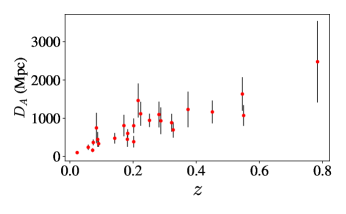
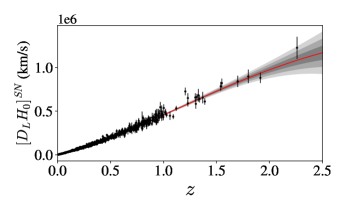
Figure 1: Left panel: Angular diameter distances to galaxy clusters. Right panel: Reconstruction of $[H_{0}D_{L}]^{SN}(z)$ from the Pantheon sample. The solid blue line and the shadowed regions represent the reconstruction central value, and the 1$\sigma$, 2$\sigma$ and 3$\sigma$ CL obtained by the GP method.

For the galaxy cluster observations, the common statistical contributions are: SZE point sources $\pm 8\%$, X-ray background $\pm 2\%$, Galactic NH $\leq\pm 1\%$, $\pm 15\%$ for cluster asphericity, $\pm 8\%$ kinetic SZ and for CMB anisotropy $\leq\pm 2\%$. Estimates for systematic effects are: SZ calibration $\pm 8\%$, X-ray flux calibration $\pm 5\%$, radio halos $\pm 3\%$ and X-ray temperature calibration $\pm 7.5\%$ (see, for instance, Table 3 Bonamente et al. (2006)). For systematics, the typical errors are around $13\%$. In the present analysis, we have combined the statistical and systematic errors in quadrature for the angular diameter distance from galaxy clusters. Therefore, Figure 1 shows the $[D_{A}]^{GC}(z)$ sample used in this paper. Through the years, this data set has been used in several contexts cosmological, such as: in cosmological parameter estimates Holanda et al. (2012a, 2013); Lee (2014); Lima and Cunha (2014), for tests of the cosmic distance duality relation Holanda et al. (2010); Liang et al. (2013); Santos-da-Costa et al. (2015); Lin et al. (2018), for tests of the fundamental physics Holanda et al. (2016); Liu et al. (2021a); Colaço et al. (2019), etc.

II.2 The unanchored luminosity distance

To obtain the absolute distance, $D_{L}(z)$, from SNe Ia it is entangled with the combination of the absolute magnitude, $M_{B}$, and the Hubble constant $H_{0}$. However, observations of SNe Ia can also provide the so-called unanchored luminosity distance $[H_{0}D_{L}(z)]$, which is the quantity we shall use for our purposes. Thus, the unanchored luminosity distances are derived from the apparent magnitude of SNe Ia by the relation:

$$m_{B}=5\log_{10}[H_{0}D_{L}(z)]-5a_{B},$$ (13)

where $m_{B}$ is the distance moduli measurements, and we assume the fixed value $a_{B}=0.71273\pm 0.00176$ as inferred by Riess et al. (2016). Such value is independent of any absolute scale, luminosity, or distance, and is determined from a Hubble diagram of SNe Ia with a light-curve fitter.

For our purpose, we shall use the Pantheon type Ia supernovae sample in order to obtain the unanchored luminosity distances, $[H_{0}{D_{L}}]^{SN}(z)$, at the redshift of the GC sample. The Pantheon compilation consists of 1048 measurements of SNe Ia apparent magnitudes, $m_{b}$, in the redshift range $0.01<z<2.3$ Scolnic et al. (2018). Then, we transform the Pantheon sample of apparent magnitudes into unanchored luminosity distances sample by considering the relation (13) via

$$[H_{0}D_{L}]^{\rm SN}(z)=10^{(m_{b}+5a_{B})/5}\equiv 10^{m_{b}^{\prime}/5}.$$ (14)

To estimate the $[H_{0}D_{L}]^{\rm SN}$ uncertainties including their correlations, we consider the covariance matrix of the apparent magnitudes (statistics+systematics) and the $a_{B}$ error. The covariance matrix of $m^{\prime}_{b}$ is obtained by:

$$\textbf{Cov}(m^{\prime}_{b})=\textbf{Cov}(mb)+(5\sigma_{a{{}_{B}}})^{2}\bm{I},$$ (15)

where $\bm{I}$ is the unity matrix. The covariance of the luminosity distance is calculated using the matrix transformation relation as follows

$$\textbf{Cov}([H_{0}D_{L}]^{SN})=$$ (16)

$$\left(\frac{\partial[\bm{H}_{0}\bm{D}_{L}]^{SN}}{\partial\bm{m}^{\prime}_{b}}\right)\textbf{Cov}(m_{b})\left(\frac{\partial[\bm{H}_{0}\bm{D}_{L}]^{SN}}{\partial\bm{m}^{\prime}_{b}}\right)^{T},$$ (17)

where $\frac{\partial[\bm{H}_{0}\bm{D}_{L}]^{SN}}{\partial\bm{m}^{\prime}_{b}}$ represents the partial derivative matrix of the unanchored luminosity distance vector $[\bm{H}_{0}\bm{D}_{L}]^{SN}$ with respect to the vector $\bm{m}^{\prime}_{b}$.

In addition, we use the Gaussian Process (GP) method trained on the SNe Ia sample to reconstruct $[H_{0}D_{L}(z)]^{SN}$ functions (see Fig. 1 (right panel)). The trained network shall be able to forecast unanchored luminosity distances at redshifts that match $[D_{A}(z)]^{GC}$ from galaxy clusters. The GP reconstruction is performed by choosing a prior mean function and a covariance function which quantifies the correlation between the values of the dependent variable of the reconstruction and is characterized by a set of hyperparameters (see Ref. Seikel and Clarkson (2013) for more details about GP). In our reconstructions of $[H_{0}D_{L}(z)]^{SN}$, we choose zero as the prior mean function to avoid biased results and a Gaussian kernel as the covariance function given by:

$$k(z,z^{\prime})=\sigma^{2}\exp\left(-\frac{(z-z^{\prime})^{2}}{2l^{2}}\right),$$ (18)

where $\sigma$ and $l$ are the hyperparameters related to the variation of the estimated function and its smoothing scale, respectively. To optimize the hyperparameter values, we maximize the logarithm of the marginal likelihood:

$$\ln{\mathcal{L}}=-\frac{1}{2}\bm{y}^{T}[k(\bm{x},\bm{x})+C]\bm{y}-\frac{1}{2}\ln|k(\bm{x},\bm{x})+C|,$$ (19)

where $\bm{x}$ and $\bm{y}$ are the vectors of the independent and dependent data variables, respectively, and $C$ is the covariance matrix of the data ($[H_{0}D_{L}(z)]^{SN}$ error matrix) calculated using the Eq. (16). We use the code GaPP to perform the GP reconstruction of the $[H_{0}D_{L}(z)]^{SN}$ function. In what follows, we discuss our main results.

III Main Results

We use Markov Chain Monte Carlo (MCMC) methods to estimate the posterior probability distribution functions (pdf) of free parameters supported by emcee MCMC sampler Foreman-Mackey et al. (2013). To perform the plots, we used the GetDist Python package. The likelihood is given by

$$\mathcal{L}(\mathrm{Data}|\vec{\Theta})=\prod\frac{1}{\sqrt{2\pi}\sigma_{\mu}}e^{-\frac{1}{2}\chi^{2}},$$ (20)

with

$$\chi^{2}=(H_{0}-H_{0}^{\mathrm{Data}}(z_{i}))\bm{C}_{H_{0}}^{-1}(H_{0}-H_{0}^{\mathrm{Data}}(z_{i}))^{T},$$ (21)

where $H_{0}^{\mathrm{Data}}$ is given by eq.(2), $H_{0}$ is the free parameter, and $\bm{C}_{H_{0}}^{-1}$ is the inverse of the covariance matrix. The pdf is proportional to the product between likelihood and prior ($P(\Theta)$), that is,

$$P(\vec{\Theta}|\mathrm{Data})\propto\mathcal{L}(\mathrm{Data}|\vec{\Theta})\times P(\vec{\Theta}).$$ (22)

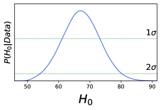
Figure 2: Posterior probability distribution functions of $H_{0}$. The green horizontal dashed lines correspond to $1\sigma$ and $2\sigma$ CL, respectively.

In our analyses, we assume flat prior: $H_{0}=[50,100]$ km/s/Mpc.

We combined the 25 points of $[D_{A}(z)]^{GC}$ with SNe Ia in order to obtain $H_{0}$. We note that the sample presented one measurement of $H_{0}$ with a very large error. This occurred when the GC MS 1137.5+6625 was considered. To avoid biases, we removed this cluster and performed the final analyses with 24 points of $D_{A}(z)-H_{0}D_{L}(z)$. After summing the statistical and systematic errors in GC measurements in quadrature in our analysis, we obtain $H_{0}=67.2\pm 6.1$ ${\rm\,km\,s^{-1}\,Mpc^{-1}}$ at $1\sigma$ CL with an error around $9\%$ (see Fig.2). Due to errors presented in galaxy cluster observations, our method provided consistent and compatible results of the Hubble parameter at low and intermediate redshifts. Moreover, this constraint is in full agreement with that one from the Planck satellite observations, but it is also compatible with the measure provided by the SHOES team. However, it is very important to stress that unlike the $H_{0}$ estimate from Renzi and Silvestri (2023), our result only depends on two types of observations, where $[D_{A}]^{GC}$ used here is completely independent of local calibrators.

IV Final Remarks

In this paper, we discussed a determination of the Hubble constant $H_{0}$, without using any cosmological model, based only on the SZE/X-ray distance technique for measuring galaxy cluster angular diameter distances and type Ia supernovae observations. We followed the method proposed in Renzi and Silvestri (2023) (see II), but only two types of astronomical measurements were considered here. In galaxy cluster observations (25 data), the electronic density of the intra-cluster medium was described by an isothermal elliptical $\beta$-model Filippis et al. (2005). For SNe Ia, we used the Pantheon sample. It was obtained $H_{0}=67.2\pm 6.1$ ${\rm\,km\,s^{-1}\,Mpc^{-1}}$ at $1\sigma$ CL. It is important to comment that the statistical and systematic errors in galaxy cluster measurements are summed in quadrature in our analysis. As one may see, the constraints on the Hubble constant derived here are consistent with the latest and conflicting measures provided by the SHOES team and the Planck satellite. This occurs due to errors present in galaxy cluster observations.

Finally, it is worth commenting that the galaxy cluster angular diameter from their SZE+X-ray observations is completely independent of any calibrator usually adopted in the determinations of the distance scale. Then, our results also reinforce the interest in the observational search for new galaxy cluster angular diameter distance samples from the SZE and X-ray observations.