DySurv: Dynamic Deep Learning Model for Survival Prediction in the ICU

Abstract

Survival analysis helps approximate underlying distributions of time-to-events which in the case of critical care like in the ICU can be a powerful tool for dynamic mortality risk prediction. Extending beyond the classical Cox model, deep learning techniques have been leveraged over the last years relaxing the many constraints of their counterparts from statistical methods. In this work, we propose a novel conditional variational autoencoder-based method called DySurv which uses a combination of static and time-series measurements from patient electronic health records in estimating risk of death dynamically in the ICU. DySurv has been tested on standard benchmarks where it outperforms most existing methods including other deep learning methods and we evaluate it on a real-world patient database from MIMIC-IV. The predictive capacity of DySurv is consistent and the survival estimates remain disentangled across different datasets supporting the idea that dynamic deep learning models based on conditional variational inference in multi-task cases can be robust models for survival analysis.

I Introduction

Survival analysis refers to statistical approaches at estimating distributions of event times or times it takes for an event to happen as well as rates of survival over time accounting for censoring. The events in question can be machine failures in industry or the occurrence of specific diseases and death [1]. In clinical practice, survival analysis can play a key role and provide valuable insights into predicting patient outcomes and guiding treatment decisions [2]. While most traditional applications of methods rely on statistical models in epidemiology, with the rise of deep learning techniques, personalised estimation of survival times for individual patients has become possible [3]. Survival analysis can provide dynamic risk estimation for a population or an individual patient over a period of time which helps track the progression of risk and when combined with comparative analysis, variation in survivability between treatment regimes. In settings like intensive care units (ICUs), such robust prediction frameworks would be especially useful. Besides, deep learning is more robust in detecting non-linear patterns in data, estimating unknown distributions, and learning from complex data modalities like time-series and images.

The primary objective of survival analysis is to approximate the underlying distribution of events or hitting times known as the survival function taking into account the influence of input features [4]. There are diverging approaches to solving this problem such as assuming a specific distribution like the Weibull for the survival function and then estimating the parameters of this distribution using specific models from deep learning [5]. Other approaches like the standard Cox Proportional Hazards (Cox) model are considered semi-parametric as they assume a specific base distribution for the hazard function (related to the survival function) which is then altered through an exponential factor of the features [6]. In most cases, however, the features are static and the models suffer under the limitations of the assumptions made like the proportional hazards assumption in the case of Cox and some of its derivatives. Using time-series deep learning models can allow for learning long-term and sequential patterns in patient data without being restricted to using just static features or just the most recent measurements while also directly estimating the survival function (or alternatives like the hazard function) through custom loss implementations.

Our work aims to address these limitations by using components like Long Short-Term Memory (LSTM) to extract relevant patterns from time-series data while capturing the long-term dependencies present in a patient’s stay in the ICU. In addition, instead of assuming a prior distribution for the survival or hazard function, we directly model the survival through an adapted negative log-likelihood loss function accounting for censoring in the data. Other deep learning implementations have used similar components like RNNs but we decide to use the advantage of variational autoencoders (VAEs) and conditional extensions which achieve superior performance in latent space generation while also being useful for generative modelling [7, 8, 9]. We aim to show that conditional variational inference and autoencoder reconstruction tasks can aid in learning from complex time-series data by extracting latent features later used in optimising the survival task. We validate our approach both in a static and time-varying settings using a combination of benchmark datasets from survival analysis as well as a recent public ICU database. The ICU remains a key component of delivering critical care where decisions need to be made urgently and whose effects can be seen within hours of the stay [10]. In such a time-sensitive environment, providing dynamic risk estimation through survival curves and time-dependent prediction can aid in prioritising patients most urgently in need of care while considering the progression of deterioration throughout the stay.

Using the fact that VAEs have been established as robust tools for probabilistic modelling capable of capturing the underlying distribution of complex high-dimensional data through learning salient low-dimensional representations, we apply them to model the relationship between covariates and survival times, enabling accurate estimation of survival probabilities and event predictions. Since the model is not just multi-modal in input but also in output with both reconstruction and survival tasks included, conditional variational autoencoders (CVAE) provide a stable prediction performance [11]. By mapping high-dimensional covariates into a lower-dimensional space, CVAEs can effectively capture the underlying structure and identify hidden factors that significantly impact survival outcomes and predict for both binary labels of mortality as well as times of death. This capability allows deeper insights into time-resolved mortality risk prediction and disease progression in critical care.

II Materials and Methods

II-A Data

Data for survival analysis contains three main sets of variables, the first is the feature set $\mathcal{X}$ which can consist of static or time-series features (the latter having measurements at potentially different sampling frequencies), the time-to-event for the events in question or censoring respectively, and the outcome label for the event like in standard machine learning tasks [12]. In all of our dataset implementations, we standardise the start time for the time-to-events to zero and for MIMIC IV we will detail further pre-processing steps. In general, the time-to-event values can be left to be continuous depending on the model being considered but we discretise the time set into 10 equally spaced time periods for our model in the fashion of DeepHit and Dynamic-DeepHit [9]. Furthermore, measurements are often right-censored, meaning that patients can leave the study or be lost to follow-up and not everyone needs to have experienced the event with their time-to-event and time-varying features reflecting this. An assumption commonly made elsewhere and here is that this censoring is unimportant and independent of the outcome of the study itself [13]. Thus, the dataset can be represented as

$$\mathcal{D}=\left\{\left(\mathcal{X}^{i},\mathcal{t}^{i},y^{i}\right)\right\}_{i=1}^{N}$$ (1)

With $\mathcal{X}$ representing the feature matrix, $\mathcal{t}$ being the time-to-event as the minimum of the event and censoring time, $y$ being the label for the outcome, and $N$ samples included. As we will be working with time-series data in the case of MIMIC-IV, a patient $\mathcal{X}^{i}$ can be seen as

$$\mathcal{X}^{i}=\left\{\boldsymbol{x}_{1}^{i},\boldsymbol{x}_{2}^{i},\ldots,\boldsymbol{x}_{j}^{i}\right\}$$ (2)

Where $j$ is the length of the time-series for $1\leq j<J^{i}$ where $J$ is the maximum time step and $\boldsymbol{x}_{j}^{i}$ contains $M$ features $\left[x_{j,1}^{i},x_{j,2}^{i},\ldots,x_{j,M}^{i}\right]^{\top}$ with timestamps of measurements $\left[t_{1}^{i},t_{2}^{i},\ldots,t_{j}^{i}\right]$.

Standard benchmark datasets contain only static features but here we implement survival analysis on the ICU dataset from MIMIC-IV which contains both static and time-series features. To show performance across different datasets and with different sizes, we will succinctly introduce these datasets. Across all datasets, the event in question is death. The datasets were split into 60% training, and 20% each for validation and testing. Quantile transformations have been applied for standardisation and fit only on the training dataset. Please see appendix for a full list of features for each dataset.

II-A1 SUPPORT

The Study to Understand Prognoses and Preferences for Outcomes and Risks of Treatments contains data from five care academic centres in the United States for general population survival for the next six months [14]. The result of the study was a prognostic model to estimate survival for seriously ill hospitalised patients. The dataset consists of 8,873 samples and 14 features.

II-A2 METABRIC

The Molecular Taxonomy of Breast Cancer International Consortium contains genetic and clinical data from breast cancer patients with 1,904 samples and 9 features [15].

II-A3 GBSG

The Rotterdam & German Breast Cancer Study Group contains treatment and clinical data on 2,232 breast cancer patients with 6 features [16].

II-A4 NWTCO

The National Wilm’s Tumor dataset contains staging and clinical data on 4,028 Wilms’ tumor patients with 6 features [17].

II-A5 sac3

The simulated dataset contains discrete time event-times with 44 features and 100,000 samples [18].

II-A6 sac_admin5

The simulated dataset contains discrete time event-times with 5 features and 50,000 samples [19].

II-A7 MIMIC IV

We also implement survival analysis on the de-identified real-world ICU dataset Medical Information Mart for Intensive Care (MIMIC-IV v. 2.0, July 2022) which includes discharge information for over 15,000 additional ICU patients compared to the previous release [20]. The dataset contains data from the Beth Israel Deaconess Medical Center collected between 2008 and 2019. The dataset contains 71,935 samples of ICU stays with 33 static features (categorical features were one-hot encoded) and 65 time-varying features. Static variables include age, sex, unit of admission, and others which did not have missingness and for the time-series we decided to use forward filling as clinicians in practice would similarly just look at the last recorded measurement. If the first set of measurements is missing for some time-varying features we backward fill for that feature for that patient so all time-series features across all patients can later be aligned to start from the beginning of admission and earliest record. Our processing of MIMIC-IV follows from our previous work but is adapted for the survival scenario with the ICU length of stay or the maximum time horizon for the event times defined as 10 days and time-series features taken in 72-hour timesteps [21].

II-B Survival Function and Losses

In survival analysis, the main underlying goal is the estimation of the survival function which represents the probability that no event occurs until a time t and can be written as

$$S(t)=\operatorname{P}(T>t)=\int_{t}^{+\infty}f(u)du=1-F(t)$$ (3)

Where $f(t)$ is the probability density function of event time

$$f(t)=\lim_{\Delta t\rightarrow 0}\frac{\operatorname{P}(t<T\leq t+\Delta t)}{\Delta t}$$

and $F(t)$ corresponds to the cumulative risk or incidence function $F(t)=\operatorname{P}(T\leq t)$. $T$ represents the time of the event, $\operatorname{P}$ is the probability, and $t$ is the specitic timestamp for risk estimation. The key to training a deep learning model is to learn an estimate of the cumulative incidence or risk function $\hat{F}(t)$ as the joint distribution of the event time and outcome label given the observations. As we discretise the time into intervals, we can estimate this event probability across arbitrary periods and remain faithful to the original survival analysis formulation instead of resorting to chained binary classification [22]. Once we have an estimate of the risk, we can then simply obtain the survival function and curves by taking its negation from one as shown in equation (3). We also discretise the time scale in the style of other popular deep learning approaches so we depend on the probability mass function instead of the probability density function.

We undertake estimation of the underlying cumulative risk by primarily optimising for the negative log-likelihood of the joint distribution of the event time and outcome with right-censoring. For those patients who have suffered the event, we capture both the outcome and the time at which it occurs. For censored patients, we capture the censoring time conditioned on the measurements recorded prior to the censoring. If we assume $a_{t}=\hat{P}\left(T=t\mid\mathcal{X}\right)$ (the output of the last layer node of the neural network module) represents the probability of experiencing the event at time $t$, then the loss can be represented as

$$\mathcal{L}_{1}=- \sum_{i=1}^{N}\left[1\left(y^{i}\neq\varnothing\right)\cdot\log\left(\frac{a_{t^{i}}^{i}}{1-\sum_{y\neq\varnothing}\sum_{n\leq t_{Ji}^{i}}a_{n}^{i}}\right)\right.$$ (4)

$$\left.+1\left(y^{i}=\varnothing\right)\cdot\log\left(1-\sum_{y\neq\varnothing}\hat{F}\left(t^{i}\mid\mathcal{X}^{i}\right)\right)\right]$$

Where $1$ is the indicator function. By optimising for this loss, we estimate the actual risk distribution for each patient and a prediction can be made for arbitrary times across event times as outputs of the last layer.

As data are complex (i.e., static and time-varying), we seek to learn a latent representation using a variational autoencoder that would improve learning for the task of survival analysis. There are two loss terms, namely the reconstruction (mean squared error) and the Kullback–Leibler (KL) divergence in the variational autoencoder. Estimating the distribution of the underlying latent factors relies on minimising the KL divergence between an approximation of the true posterior and the true distribution both of which are assumed to be multivariate Gaussians. As such, learning these distributions means optimising for their parameters, the mean and standard deviation. The ability of the decoder to successfully reconstruct the input is captured with a simple mean squared error term between the reconstruction of the input and the input itself. Thus, the loss for variational inference can be seen as

$$\mathcal{L}_{2}=L_{vae}(E,D)=\left\|\mathcal{X}-\mathcal{X}_{\text{recon }}\right\|_{2}$$ (5)

$$+\frac{1}{2}\sum_{i=1}^{z_{\text{dim }}}[\left(\mu_{i}^{2}+\sigma_{i}^{2}\right)-1-\log\left(\sigma_{i}^{2}\right))]$$

Where $z$ is the sampled latent vector from the probabilistic encoder for the learned Gaussian distribution with mean $\mu$ and standard deviation $\sigma$. For training, however, since sampling is a stochastic process, we use the reparameterization trick to backpropagate the gradient and represent the latent vector as the sum of a deterministic variable and an auxiliary independent random variable $\varepsilon$ [23]

$$\varepsilon\sim N(0,1)\quad z=\mu+\varepsilon*\sigma\quad\rightarrow\quad z\sim N(\mu,\sigma)$$ (6)

This latent vector is then used as input to a neural network module in learning the survival task. During training, the decoder uses the latent vector and the condition vector (survival labels or times of death) as input which helps the latent space capture other information instead of trying to better reconstruct the input. At test time, the decoder is not used anymore, and the latent space is used for prediction in the survival task. Details on the network structure implementing the optimisation will be discussed later, but the total loss can then be presented as

$$\mathcal{L}=\alpha\mathcal{L}_{1}+(1-\alpha)\mathcal{L}_{2}$$ (7)

Where $\alpha$ is the balancing coefficient between the two losses ($\mathcal{L}_{1}$ and $\mathcal{L}_{2}$) and $0\leq\alpha\leq 1$. $\alpha$ is considered as a hyperparameter that is optimised during training according to multi-objective optimization principles.

II-C Benchmark Models

To compare DySurv to other survival analysis methods, we implement a selection of the most popular and consistently cited methods in the field and provide a short description of each below. We will first introduce discrete-time methods which rely on discretising the event times into specified durations, and then follow with continuous-time methods.

II-C1 PMF

The parametrisation of the Probability Mass Function (PMF) of the event times is another way of estimation without resorting to using discrete-time risk or hazard in likelihood optimisation. We described the continuous probability density function without using discrete time boundaries. It is the foundation of other methods like DeepHit and Multi-Task Logistic Regression. It similarly resorts to optimising a negative log-likelihood loss but instead of using the cumulative risk function, it uses the approximations of the PMF and survival functions [18]. Since we can establish a direct representational relation between the risk and survival functions, the PMF loss can be seen as an alternative to our own loss function. In our and others’ implementation, the PMF method is a simple Multi-Layer Perceptron (MLP) optimised for this loss and we use the same structure as we use for our survival module to be described later.

II-C2 MTLR

Multi-Task Logistic Regression provides a generalization of the binomial log-likelihood to jointly model the sequence of binary labels for each time interval risk prediction. This method similarly minimises the negative log-likelihood with the PMF and survival function terms but the network outputs are cumulatively summed in reverse to no certain advantage and, in fact, just adds computational complexity and numeric instability [24, 25].

II-C3 BCESurv

This Binary Cross-Entropy for Survival is a method consisting of a set of binary classifiers that remove individuals as they are censored. The loss is the binary cross entropy of the survival estimates at a set of discrete times, with targets that are indicators of surviving each time. Each output node in the last layer corresponds to a binary classifier evaluated at that time point. As censored patients are removed, the method is biased towards those with higher event probabilities [19].

II-C4 DeepHit

The single-risk version of DeepHit is a deep learning model whose output nodes are softmaxed to jointly model the probabilities between the event times and the time durations are discretised like in our case. The model depends on optimising both the negative log-likelihood loss based on the cumulative incidence function and a ranking loss built on the intuition of the concordance. The ranking loss penalises incorrect ordering of patient pairs in which the patient that remains longer in the study should have a lower risk at the end point for the patient with the shorter stay. Including this loss function allows the model to directly optimise for the concordance metric which is also the only metric of evaluation used in their paper hence leading to potentially biased and inflated results. Subsequently reproduced work has shown that indeed this model is not calibrated well and the inclusion of this ranking loss, while helping to show better performance as measured by concordance, significantly lags across other metrics in survival analysis when compared to simpler models [26, 8, 22, 27].

II-C5 Logistic Hazard

The Logistic Hazard method is a submodular implementation of our own deep learning model using the loss in (4) with an MLP that similarly parametrises the PMF of the survival times [28]. DySurv expands on this method to include it as a component in the framework with the variational autoencoder to jointly optimise for both tasks of reconstruction and latent space formation as well as survival estimation. A key difference between the log-likelihood loss used here (and in our model) and in DeepHit is that logistic hazards do not allow for survival past the maximum time horizon.

II-C6 CoxTime

CoxTime is a relative risk model that extends Cox regression beyond the proportional hazards and is the first of the continuous-time methods. The standard Cox regression model which we will not spend space introducing here consists of a baseline hazard term (defined cumulatively in the loss by a pre-selected estimator such as Breslow) and a relative risk term which is an exponential factor of the weighted linear combination of features. The basic model assumes constant proportionality between the patients’ hazards over time and is thus restrictive. In other words, the difference between survival likelihoods for a given time is proportional to the difference in feature or hazard values for patients. CoxTime goes around this assumption by parametrising the relative risk term as a function of time and not just the features, thus the non-proportional behaviour over time is modelled by allowing for time to be considered alongside the features [29].

II-C7 CoxCC

CoxCC (Case Control) is just a proportional implementation of the CoxTime model and is the closest to the standard Cox implementation where the minimisation of the partial log-likelihood is done with stochastic gradient descent by averaging over constrained risk sets for mini-batch learning instead of the entire dataset like in classical survival analysis [29].

II-C8 DeepSurv

DeepSurv is a deep learning model that directly minimises the negative partial log-likelihood as defined in the standard Cox model. It is one of the first deep learning implementations for survival analysis and the output of the model is the log-risk term of the Cox model which accounts for nonlinearity [30]. There is no indirect estimation of cumulative risk or survival through likelihood estimation like in the previous methods, thus DeepSurv similarly suffers under limitations of the Cox such as the proportionality assumption [31].

II-C9 PCHazard

The last continuous-time method we introduce and implement is PCHazard which assumes that the continuous-time hazard rate (instantaneous value of risk) is piecewise constant. The method relies on optimising for the likelihood contribution which mimics the MTLR approach albeit in the continuous-time setting with the hazards parametrised by a simple MLP. The piecewise constant causes the likelihood to behave like a Poisson likelihood [32]. Despite the method operating in continuous-time, the hazards are defined in time intervals which rely on discretisation steps from the observed continuous event times and censoring times, while we discretise the times to a predefined set of time flagposts [18].

A summary of all the methods can be seen in Table I.

TABLE I: Survival analysis methods investigated

Method	Time scale	Reference
PMF	discrete-time	[18]
MTLR	discrete-time	[24]
BCESurv	discrete-time	[19]
DeepHit	discrete-time	[26]
Logistic Hazard	discrete-time	[28]
CoxTime	continuous-time	[29]
CoxCC	continuous-time	[29]
DeepSurv	continuous-time	[30]
PCHazard	continuous-time	[18]

II-D DySurv

Our proposed deep learning model leverages the established structure of a variational autoencoder and combines it with a survival analysis learning MPL module to simultaneously optimise for both reconstruction and likelihood losses. Figure 1 shows the structure of the proposed model. Using a simple autoencoder has been shown to lead to overfitting and imbalanced learning of the reconstruction task that could harm learning the survival task whereas a VAE’s objective function is based on the reconstruction loss from a randomly sampled vector allowing for more robustness [33]. We concatenate the feature vectors from the static and time-series features together before feeding them into an encoder equipped with a Long-Short Term Memory (LSTM) cell. As mentioned earlier, we use 72 1-hour timesteps and static variables are included by replicating them before concatenation with the time-series vector. Indeed, the time-series components are compressed into a latent representation which is then used, as is, as input to the estimation of the negative log-likelihood loss function. Following the LSTM unit, the remaining part of the encoder consists of an MLP module with 3 layers. The encoder and decoder are mirrored in their structure with the hidden neurons in the MLP layers consisting of 3 times feature length, then 5 times, then 3 times, before passing onto the last output layer. For the encoder, the last layer is used in approximating the mean and standard deviation of the latent Gaussian distribution. As for the decoder, the last output layer is used for reconstructing the input vector. Once the latent vector is sampled from the Gaussian distribution defined by these parameters, the lower-dimensional latent factors are used as input for an MLP module in optimising the survival task. The survival module is similar to the MLP components of the encoder and decoder. All components are jointly optimised through multi-loss optimisation. All of the components have been investigated with and without dropout included. The output of the survival module is 10 nodes softmaxed hence properly jointly distributed, each of which gives the probability that the patient has suffered the event (death) at that specific time interval. In the MIMIC-IV case, each node then corresponds to 1-day risk prediction in the ICU as the maximum time horizon is 10 days. The hyperparameters optimised in the network through grid search using the training and validation set included learning rate, batch size, $\alpha$, and dropout proportion. To minimise overfitting, we employ early stopping techniques.

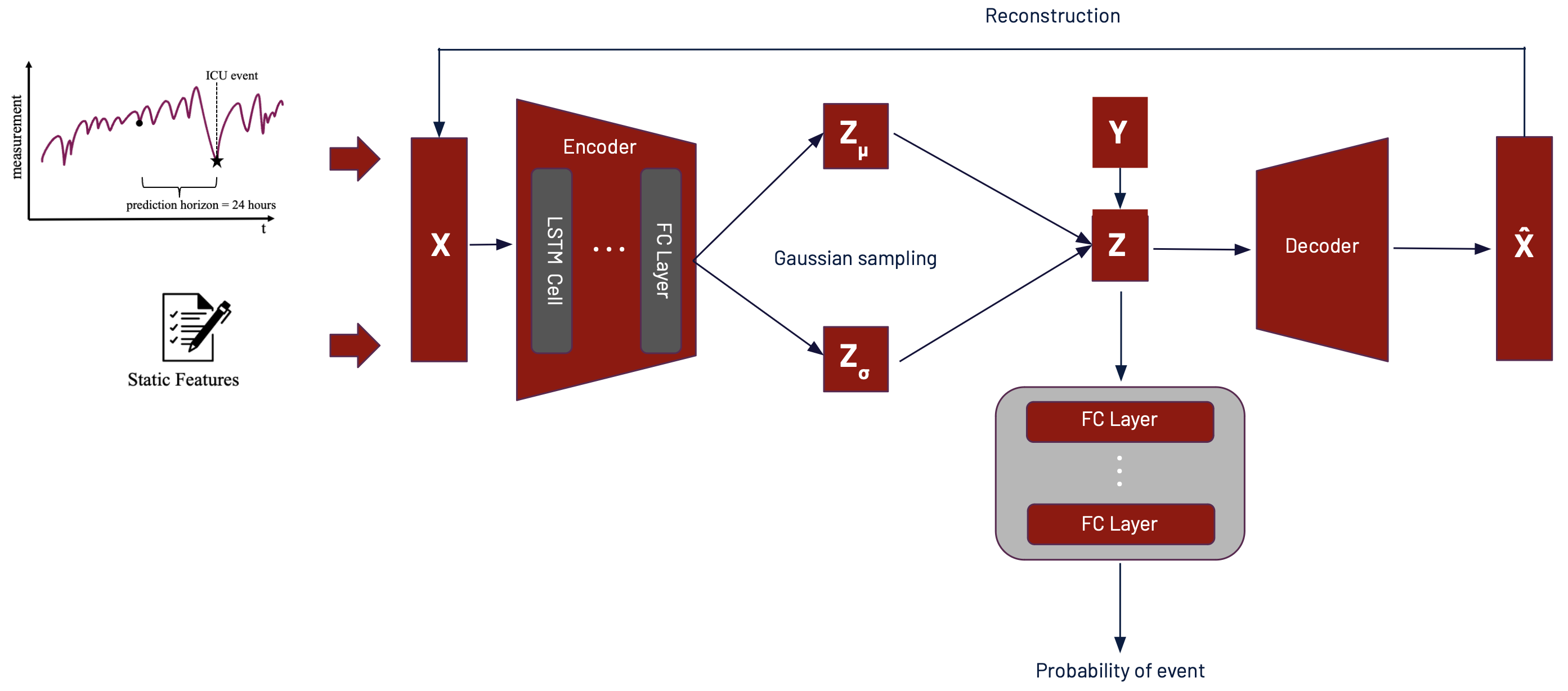
Figure 1: Proposed DySurv model for dynamic risk prediction based on a combination of static and time-series EHR data

II-E Metrics

In this section, we will switch the notation of samples from superscript to subscript, hence $\mathbf{x}^{i}$ is now $\mathbf{x}_{i}$ for sample $i$. Since we are no longer making single risk predictions at specific times and estimating distributions of event times for censored samples, different evaluation metrics must apply than those used in classic machine learning classification and prediction settings. The most common metric for evaluating survival analysis models is the concordance index $C_{ind}$, which estimates the probability that, for a random pair of samples, the predicted survival times (risk probabilities) of the two samples have the same ordering as their true survival times [29]. This explanation works perfectly for settings of proportional hazards where the ordering does not change over time but for our purposes, we will not be limited by such assumptions. Hence, we will rely on using the time-dependent extension $C_{ind}^{\mathrm{td}}$ with some modifications accounting for predictions independent of feature observations having a concordance of 0.5. The metric can be represented as

$$C_{ind}^{\mathrm{td}}=\mathrm{P}\left\{\hat{S}\left(T_{i}\mid\mathbf{x}_{i}\right)<\hat{S}\left(T_{i}\mid\mathbf{x}_{j}\right)\mid T_{i}<T_{j},D_{i}=1\right\}$$ (8)

Where $\hat{S}$ indicates the estimated survival probabilities are used and $D_{i}=1$ that only those who experienced the event are considered in this metric. A noted limitation of this metric is its obvious bias and dependence on the censoring distribution as only non-censored samples are considered making it affected by the length of stay and the censoring proportion that increases over the length of stay. To this end, we decide to use additional metrics for more holistic evaluation especially as previously proposed models like DeepHit were found to be ungeneralisable when evaluated using other metrics besides concordance. We also evaluate our model using the Integrated Brier Score or IBS. The Brier Score is similar to the mean squared error as it represents the average squared distances between the predicted and the true survival probability (approximated with step functions with jumps at the event times) and is always a number between 0 and 1, with 0 being the best possible value [25]. In fact, the expectation of the Brier Score contains the mean squared error as one of its additive terms, so minimising one is minimising the other [19]. Since we need to know the event times for calculating IBS and we do not have access to all the samples’ event times in right-censoring, an adjusted metric called the inverse probability of censoring weights Brier Score (IPCW) is used instead to approximate the times by weighting the scores of the observed event times by the inverse probability of censoring. The equation used is thus

$$\operatorname{BS}_{\operatorname{IPCW}}(t)=\frac{1}{n}\sum_{i=1}^{n}[\frac{\hat{S}_{i}(t)^{2}1\left\{T_{i}\leq t,D_{i}=1\right\}}{\hat{G}_{i}\left(T_{i}-\right)}+$$ (9)

$$\frac{\left[1-\hat{S}_{i}(t)\right]^{2}1\left\{T_{i}>t\right\}}{\hat{G}_{i}(t)}]$$

Where $\hat{G}_{i}(t)=\mathrm{P}\left(C_{i}^{*}>t\right)>0$ is the Kaplan-Meier estimate of the censoring distribution for sample $i$ and $C_{i}^{*}$ is the censoring time. The expected value of this metric is the same as for the uncensored Brier Score. As one notices, this metric is evaluated at specific times whereas the Integrated Brier Score or IBS provides a general evaluation of model performance at all times

$$\mathrm{IBS}=\frac{1}{\max\left(T_{i}\right)}\int_{0}^{\max\left(T_{i}\right)}BS_{\operatorname{IPCW}}(t)dt$$ (10)

But a limitation of this metric is the biased assumption of the censoring distribution estimated by the nonparametric Kaplan-Meier estimator which disregards the features, meaning all samples are assumed to have the same censoring distribution. This can be addressed by using an administrative extension of the metric that requires access to all the censoring times but a discussion of this is left to the reader to peruse as they see fit [19]. Lastly, we introduce the IPCW (negative) binomial log-likelihood or NBLL from classic binary classification which measures both discrimination and calibration of the estimates and use its integrated extension for all times INBLL

$$\operatorname{BLL}(t)=\frac{1}{N}\sum_{i=1}^{N}[\frac{\log\left[1-\hat{S}\left(t\mid\mathbf{x}_{i}\right)\right]1\left\{T_{i}\leq t,D_{i}=1\right\}}{\hat{G}\left(T_{i}\right)}+$$ (11)

$$\frac{\log\left[\hat{S}\left(t\mid\mathbf{x}_{i}\right)\right]1\left\{T_{i}>t\right\}}{\hat{G}(t)}]$$

$$\mathrm{IBLL}=\frac{1}{\max\left(T_{i}\right)}\int_{0}^{\max\left(T_{i}\right)}\operatorname{BLL}(t)dt$$ (12)

For both of the last metrics, we approximate the integrals by numerical integration (for 100 timesteps as based on previous literature), and the time span is the duration of the test set as these metrics are only evaluated on the test set [29].

III Results

To holistically evaluate DySurv, we present a set of experiments and comparisons with other benchmark survival analysis models across multiple datasets. We not only present the discriminative performance of the model as measured by concordance, but also its calibration as measured by IBS and IBLL. As the main aim of the model is to issue dynamic survival scores for patients in the ICU, inclusion of the real-world MIMIC-IV electronic health records dataset provides the paper with practical significance in addition to a methodological contribution. The results consist of two major experiments, one is the ability of the model to successfully learn from static data which is present in all the datasets, and the other to learn from a combination of static and time-varying data such as MIMIC-IV. For these purposes, Dynamic-DeepHit is the only relevant comparison as other survival analysis models deal with static data only. Tables II and III show these results across datasets and for all models included. We implemented these methods in PyTorch (PyCox) v. 1.10.1 using a MacBook Air M1 2021 laptop with data processing completed using pandas and SQL.

TABLE II: Test results on different datasets for survival analysis models and DySurv as evaluated by three different metrics introduced in Materials and Methods. For concordance, higher is better, and for the other two metrics, lower is better. All of the results are an average of five random seeds.

	$C_{ind}^{\mathrm{td}}$	IBS	IBLL		$C_{ind}^{\mathrm{td}}$	IBS	IBLL
SUPPORT				METABRIC
PMF	57.9	0.195	0.574	PMF	63.8	0.168	0.497
MTLR	55.3	0.205	0.775	MTLR	56.8	0.172	0.527
BCESurv	55.3	0.290	2.08	BCESurv	56.8	0.138	0.477
DeepHit	57.3	0.273	0.678	DeepHit	65.5	0.123	0.415
Logistic Hazard	53.5	0.206	0.762	Logistic Hazard	59.0	0.163	0.498
CoxTime	59.5	0.193	0.565	CoxTime	65.4	0.114	0.361
CoxCC	59.7	0.192	0.563	CoxCC	65.9	0.166	0.508
DeepSurv	60.6	0.190	0.559	DeepSurv	62.4	0.176	0.541
PCHazard	55.1	0.206	0.633	PCHazard	51.4	0.160	0.547
DySurv	64.7	0.190	0.561	DySurv	64.5	0.120	0.387
GBSG				NWTCO
PMF	68.5	0.179	0.528	PMF	69.7	0.122	0.389
MTLR	65.6	0.180	0.542	MTLR	66.8	0.109	0.403
BCESurv	65.6	0.156	0.481	BCESurv	69.1	0.108	0.393
DeepHit	68.1	0.174	0.514	DeepHit	71.1	0.118	0.348
Logistic Hazard	67.4	0.179	0.537	Logistic Hazard	66.5	0.108	0.396
CoxTime	68.4	0.171	0.510	CoxTime	70.7	0.110	0.343
CoxCC	59.6	0.205	0.597	CoxCC	70.3	0.110	0.373
DeepSurv	68.5	0.180	0.531	DeepSurv	68.3	0.115	0.391
PCHazard	55.8	0.182	0.574	PCHazard	60.2	0.118	0.465
DySurv	70.4	0.164	0.499	DySurv	70.3	0.111	0.347
sac3				sac_admin5
PMF	74.3	0.125	0.391	PMF	71.5	0.124	0.387
MTLR	65.0	0.124	0.539	MTLR	65.7	0.122	0.520
BCESurv	67.8	0.163	0.586	BCESurv	68.4	0.164	0.505
DeepHit	74.2	0.184	0.527	DeepHit	71.6	0.186	0.396
Logistic Hazard	72.0	0.120	0.492	Logistic Hazard	70.7	0.118	0.481
CoxTime	78.7	0.117	0.362	CoxTime	78.5	0.117	0.362
CoxCC	76.4	0.124	0.384	CoxCC	76.7	0.122	0.381
DeepSurv	76.1	0.126	0.390	DeepSurv	77.4	0.119	0.371
PCHazard	64.0	0.135	0.514	PCHazard	65.1	0.123	0.503
DySurv	80.6	0.112	0.359	DySurv	79.6	0.116	0.361

TABLE III: Test results on MIMIC-IV dataset for survival analysis models and DySurv as evaluated by three different metrics introduced in Materials and Methods. For concordance, higher is better, and for the other two metrics, lower is better. All of the results are an average of five random seeds.

	$C_{ind}^{\mathrm{td}}$	IBS	IBLL
MIMIC-IV
PMF	50.9	0.126	0.389
MTLR	52.4	0.126	0.389
BCESurv	52.2	0.157	0.473
DeepHit	54.4	0.137	0.421
Logistic Hazard	52.6	0.122	0.396
CoxTime	53.1	0.122	0.337
CoxCC	52.9	0.123	0.393
DeepSurv	54.2	0.128	0.403
PCHazard	51.0	0.122	0.378
DySurv (static)	55.7	0.111	0.360
Dynamic-DeepHit	56.0	0.143	0.376
DySurv ($+$ time-series)	57.9	0.122	0.320

In survival analysis, it is also vital to show the performance of the models in creating survival curves, or estimates of the survival probabilities over time for different patients. Whereas traditional survival analysis models from statistics rely on risk sets and computing survival estimates for a population, an advantage of deep learning models is that the task of survival estimation can apply to an individual patient sample. We provide survival curves for a random group of five samples/patients across all datasets that show a clear separation of risk (entanglement indicates the model has not successfully learned the risk trajectories) for different samples as generated by DySurv. Figure 2 indicates these for all the datasets except MIMIC-IV considered.

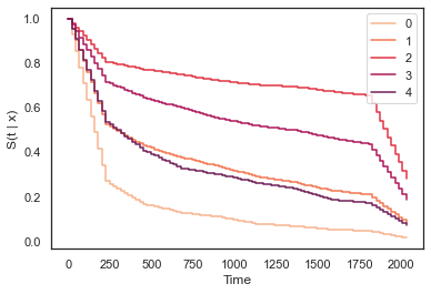
(a) Survival curve (estimate of survival probability over time) for five random samples from SUPPORT

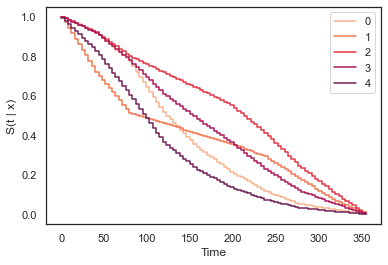
(b) Survival curve (estimate of survival probability over time) for five random samples from METABRIC

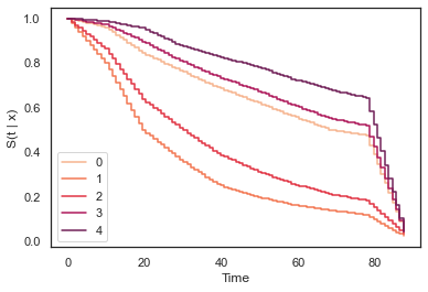
(c) Survival curve (estimate of survival probability over time) for five random samples from GBSG

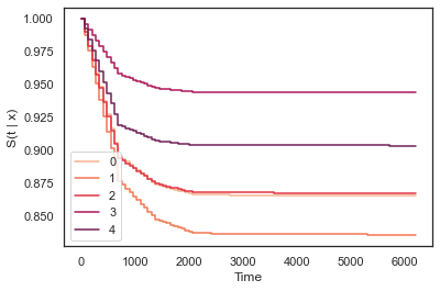
(d) Survival curve (estimate of survival probability over time) for five random samples from NWTCO

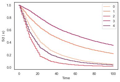
(e) Survival curve (estimate of survival probability over time) for five random samples from sac3

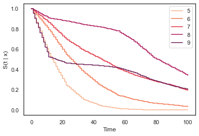
(f) Survival curve (estimate of survival probability over time) for five random samples from sac5

Figure 2: The set of survival curves for benchmark datasets as generated by DySurv that shows clear extrapolation of risk across different samples. Since DySurv provides discrete estimates over time-intervals, the curves were generated with additional interpolation commonly used in other discrete methods in survival analysis.

For MIMIC-IV, the data input consists of both static and time-series data. Here we provide survival curve results for both cases as well as for Dynamic-DeepHit in the time-series case and show how DySurv has greater capacity at separating risk trajectories in both cases as Figure 3 shows.

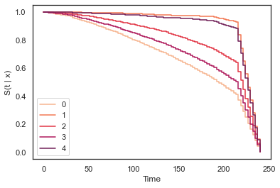
(a) Survival curve (estimate of survival probability over time) for five random samples from MIMIC-IV using only static features with DySurv

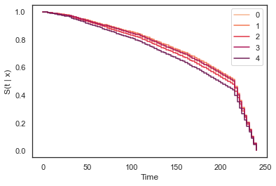
(b) Survival curve (estimate of survival probability over time) for five random samples from MIMIC-IV using both static and time-series features with DySurv

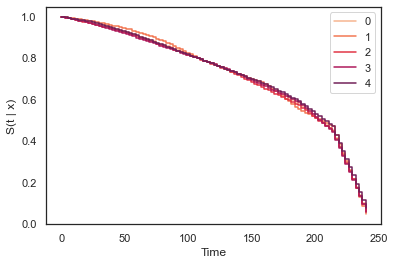
(c) Survival curve (estimate of survival probability over time) for five random samples from MIMIC-IV using both static and time-series features with Dynamic-DeepHit

Figure 3: The set of survival curves for MIMIC-IV ICU EHR dataset as generated by DySurv that shows clear extrapolation of risk across different patients as compared to both static, time-series, and Dynamic-DeepHit cases. The same set of patients was used in generating the survival curves across cases.

Upon deployment of a trained model, DySurv can generate risk estimates through time for each patient while using their history of observations. We do not rely on using landmarking methods or a specific pre-defined time for risk prediction as the score are issued across the entire time interval simultaneously. For data pre-processing purposes, a time horizon is selected corresponding to 24 hours with 72-hour timespan for the LSTM in the case of MIMIC-IV since ICU risk assessments often use information over 72 hours for the next 24-hour risk prediction [34].

IV Discussion

The first set of results relates to applying DySurv only on static data from several benchmark datasets of varying sizes. We see that for the vast majority of these benchmarks, DySurv outperforms both standard statistical as well as deep learning alternatives across all metrics except for METABRIC and NWTCO on the concordance where DeepHit tends to perform slightly better. This is probably due to the implementation of the biased ranking loss mentioned earlier that aids in having better discriminative performance as measured by the concordance metric but that is not reflected as measured by the other two metrics. Similar behaviour for DeepHit has been oberved in another study by [29]. We also see that the non-VAE implementation of the logistic hazard performs much worse than DySurv across all experiments, thereby strengthening the idea that adding variational inference to the logistic hazard can aid in learning the survival task. This improvement occurs despite having the additional task of reconstruction now. The predictive advantage comes from the identification of lower dimensional latent vectors used in the survival task instead of the raw features directly. Furthermore, on very large synthetic datasets, such as sac3 and sac_admin5, DySurv performs better due to having a greater amount of data to learn from. A limitation of the other benchmark datasets is their relatively small size may constrain DySurv from learning its optimal parameters to provide netter survival prediction.

While there are previous models that have attempted to use autoencoders for survival analysis such as [33] and [35], they have not explored variational inference extensively. These models also rely on optimisation of the Cox partial log-likelihood loss, hence being restricted by the proportionality assumption and they do not account for dynamic time-series or time-varying features in the input. Furthermore, work by [33] suggests that the VAE model’s learned compact latent representation directly aids in the Cox model’s improved performance. This intuition is precisely what we have also seen in our results albeit on a larger, more flexible, and more complex scenario of time-series ICU risk prediction with direct joint distribution estimation. The concatenation autoencoder from [35] is not even compatible with static data, by far the most common modality in survival analysis, thereby limiting its relevance significantly. DySurv addresses all these limitations and provides a flexible solution to dynamic survival analysis with deep learning.

As for MIMIC-IV results, we see that even with only static data in the input, DySurv manages to outperform other survival analysis models. When time-series data is added to the input in multi-modal fashion, it can help the model improve its performance and outperform both CoxTime and Dynamic-DeepHit across all metrics. Survival curves in Figure 3 show clearly that the static version of DySurv has the clearest separation of survival trajectories for different patients and that adding time-series data makes the task more complex. This is probably due to the reconstruction task being a lot more difficult now that time-series are involved and the model makes sacrifices on the survival task front. Nonetheless, compared to Dynamic-DeepHit whose survival curves are barely disentangled and hence unusable, the time-series version of DySurv still provides relatively reliable survival estimation. We also see that, as we would expect clinically, the survival of the patients significantly changes in the last few days in the ICU, starting to drop a few days before death. Previous work has shown that earlier times in the ICU correspond with higher survival rates. This suggests that the identification of the time period when survival rates drop dramatically in the ICU can help with targetting earlier treatment for those most at risk [36]. Patient deterioration of this kind in the ICU can help aid physicians in emergency medicine in identifying those patients most at risk in the future and proactively addressing their needs.

In this paper, we present a novel dynamic risk prediction model for survival in the ICU based on deep learning in survival analysis paradigms. Our method builds on a combination of previous work including Dynamic-DeepHit by leveraging direct learning of the joint distribution of the first event time and the event through log-likelihood optimisation with logistic hazards. Theoretically, this approach is an alternative to the risk log-likelihood loss function of Dynamic-DeepHit itself that does not use a ranking loss for biased inflation of concordance results. Our DySurv model is capable of learning from complex EHR ICU time-series data and extracting lower-dimensional latent representations that can be useful for learning the survival task while also balancing reconstruction. As the model has been difficult to train due to loss instabilities and sensitivity to hyperparameter selection, future work can explore including a regularisation component to the loss terms. And finally, using the underlying latent distribution to directly model an alternative of the survival distribution like the Weibull distribution instead of using a Gaussian intermediate.

V Contributions

MM and TZ conceived and designed the study. The data was curated by MM. Formal analysis was undertaken by MM. Development of the statistical analysis and machine learning methodologies was completed by MM. Supervision was provided by PW and TZ. Visualisations, writing, and editing was done by MM. The corresponding author and TZ had full access to all data.

VI Data sharing

The data used in the study is all publicly available. MIMIC-IV can be accessed after some initial requests and approvals from the PhysioNet website. The remaining datasets have their sources listed in the PyCox library repository.

VII Acknowledgements

Appendix A Appendix

A-A Data Description

A detailed list of features used in the study from different datasets can be seen in Tables IV and V.

TABLE IV: Features extracted from the bechmark survival datasets.

Feature	Type	Feature	Type
Sex	binary	NWTCO
Age	integer	Age	integer
Number of comorbidities	integer	Relapse	binary
SUPPORT Coma Score	continuous	Histology Local	binary
Years of Education	continuous	Histology Institute	binary
APS III Score	continuous	Tumor Stage	categorical
Diabetes	binary	Study Type	categorical
Dementia	binary	GBSG
3rd Day MAP	continuous	Age	integer
3rd Day WBC	continuous	Hormone Treatment	binary
3rd Day HR	continuous	Menopause Treatment	binary
3rd Day RR	continuous	Tumor Grade	categorical
Temperature	continuous	Number of positive nodes	categorical
3rd Day Bilirubin	continuous	Progesterone (fmol)	continuous
METABRIC		Estrogen (fmol)	continuous
Age	integer
Gene I	binary
Gene II	binary
Gene III	binary
Gene IV	binary
Hormone Treatment	binary
Radiotherapy	binary
Chemotherapy	binary
ER-positive	binary

TABLE V: Features extracted from the MIMIC-IV database. The features include demographic data collected for all patients, ICU unit-specific information like type of unit, hospital information like regional location, time since admission, vital signs including respiratory rate and blood pressure, and biochemical measurements including blood glucose and hemoglobin.

Feature	Type	Feature	Type
Sex	binary	Braden Score	continuous
Age	integer	Strength L Arm	continuous
Height	continuous	Strength R Arm	continuous
Weight	continuous	Strength L Leg	continuous
Hour of Admission	integer	Strength R Leg	continuous
Time Since Admission	continuous	GCS - Eye	continuous
Eye Response	continuous	GCS - Motor	continuous
Motor Response	continuous	GCS - Verbal	continuous
Verbal Response	continuous	Daily Weight	continuous
Ethnicity	categorical	ALT	continuous
Unit Type	categorical	AST	continuous
Admission Location	categorical	HCO3	continuous
Insurance	categorical	Hct	continuous
Time-series (summary features)
ALT	continuous	Alkaline Phosphatase	continuous
Anion Gap	continuous	AST	continuous
Base Excess	continuous	Bicarbonate	continuous
Bilirubin	continuous	Calcium	continuous
Total CO2	continuous	Chloride	continuous
Creatinine	continuous	Glucose	continuous
Hematocrit	continuous	Hemoglobin	continuous
INR(PT)	continuous	Lactate	continuous
MCH	continuous	MCHC	continuous
MCV	continuous	Magnesium	continuous
PT	continuous	PTT	continuous
Phosphate	continuous	Platelet Count	continuous
Potassium	continuous	RDW	continuous
Red Blood Cells	continuous	Sodium	continuous
Urea Nitrogen	continuous	White Blood Cells	continuous
pCO2	continuous	pH	continuous
pO2	continuous	JH-HLM	continuous
Dyspnea Assessment	continuous	Daily Weight	continuous
Glucose	continuous	Heart Rate	continuous
DBP	continuous	SBP	continuous
O2 Flow	continuous	O2 Sat (%)	continuous
Pain Level	continuous	Pain Level Response	continuous
Phosphorous	continuous	Respiratory Rate	continuous
Richmond-RAS Scale	continuous	Temperature (∘F)	continuous

References

- [1] Lee MLT, Whitmore GA. Threshold regression for survival analysis: modeling event times by a stochastic process reaching a boundary. Statistical Science. 2006.
- [2] Yoon J, Alaa A, Cadeiras M, Van Der Schaar M. Personalized donor-recipient matching for organ transplantation. In: Proceedings of the AAAI Conference on Artificial Intelligence. vol. 31; 2017. .
- [3] Luck M, Sylvain T, Cardinal H, Lodi A, Bengio Y. Deep learning for patient-specific kidney graft survival analysis. arXiv preprint arXiv:170510245. 2017.
- [4] Singh R, Mukhopadhyay K. Survival analysis in clinical trials: Basics and must know areas. Perspectives in clinical research. 2011;2(4):145.
- [5] Liu X. Survival analysis: models and applications. John Wiley & Sons; 2012.
- [6] Lin H, Zelterman D. Modeling survival data: extending the Cox model. Taylor & Francis; 2002.
- [7] Giunchiglia E, Nemchenko A, van der Schaar M. Rnn-surv: A deep recurrent model for survival analysis. In: Artificial Neural Networks and Machine Learning–ICANN 2018: 27th International Conference on Artificial Neural Networks, Rhodes, Greece, October 4-7, 2018, Proceedings, Part III 27. Springer; 2018. p. 23-32.
- [8] Ren K, Qin J, Zheng L, Yang Z, Zhang W, Qiu L, et al. Deep recurrent survival analysis. In: Proceedings of the AAAI Conference on Artificial Intelligence. vol. 33; 2019. p. 4798-805.
- [9] Lee C, Yoon J, Van Der Schaar M. Dynamic-deephit: A deep learning approach for dynamic survival analysis with competing risks based on longitudinal data. IEEE Transactions on Biomedical Engineering. 2019;67(1):122-33.
- [10] Dummitt B, Zeringue A, Palagiri A, Veremakis C, Burch B, Yount B. Using survival analysis to predict septic shock onset in ICU patients. Journal of Critical Care. 2018;48:339-44.
- [11] Itkina M, Ivanovic B, Senanayake R, Kochenderfer MJ, Pavone M. Evidential sparsification of multimodal latent spaces in conditional variational autoencoders. Advances in Neural Information Processing Systems. 2020;33:10235-46.
- [12] Bradburn MJ, Clark TG, Love SB, Altman DG. Survival analysis part II: multivariate data analysis–an introduction to concepts and methods. British journal of cancer. 2003;89(3):431-6.
- [13] Tsiatis AA, Davidian M. Joint modeling of longitudinal and time-to-event data: an overview. Statistica Sinica. 2004:809-34.
- [14] Knaus WA, Harrell FE, Lynn J, Goldman L, Phillips RS, Connors AF, et al. The SUPPORT prognostic model: Objective estimates of survival for seriously ill hospitalized adults. Annals of internal medicine. 1995;122(3):191-203.
- [15] Curtis C, Shah SP, Chin SF, Turashvili G, Rueda OM, Dunning MJ, et al. The genomic and transcriptomic architecture of 2,000 breast tumours reveals novel subgroups. Nature. 2012;486(7403):346-52.
- [16] Schumacher M, Bastert G, Bojar H, Hübner K, Olschewski M, Sauerbrei W, et al. Randomized 2 x 2 trial evaluating hormonal treatment and the duration of chemotherapy in node-positive breast cancer patients. German Breast Cancer Study Group. Journal of Clinical Oncology. 1994;12(10):2086-93.
- [17] Breslow NE, Chatterjee N. Design and analysis of two-phase studies with binary outcome applied to Wilms tumour prognosis. Journal of the Royal Statistical Society: Series C (Applied Statistics). 1999;48(4):457-68.
- [18] Kvamme H, Borgan Ø. Continuous and discrete-time survival prediction with neural networks. arXiv preprint arXiv:191006724. 2019.
- [19] Kvamme H, Borgan Ø. The brier score under administrative censoring: Problems and solutions. arXiv preprint arXiv:191208581. 2019.
- [20] Johnson A, Bulgarelli L, Pollard T, Horng S, Celi LA, Mark R. Mimic-iv. version 04) PhysioNet https://doi org/1013026/a3wn-hq05. 2020.
- [21] Mesinovic M, Watkinson P, Zhu T. XMI-ICU: Explainable Machine Learning Model for Pseudo-Dynamic Prediction of Mortality in the ICU for Heart Attack Patients. arXiv preprint arXiv:230506109. 2023.
- [22] Sun Z, Dong W, Shi J, He K, Huang Z. Attention-based deep recurrent model for survival prediction. ACM Transactions on Computing for Healthcare. 2021;2(4):1-18.
- [23] Kingma DP, Welling M. Auto-encoding variational bayes. arXiv preprint arXiv:13126114. 2013.
- [24] Yu CN, Greiner R, Lin HC, Baracos V. Learning patient-specific cancer survival distributions as a sequence of dependent regressors. Advances in neural information processing systems. 2011;24.
- [25] Fotso S. Deep neural networks for survival analysis based on a multi-task framework. arXiv preprint arXiv:180105512. 2018.
- [26] Lee C, Zame W, Yoon J, Van Der Schaar M. Deephit: A deep learning approach to survival analysis with competing risks. In: Proceedings of the AAAI conference on artificial intelligence. vol. 32; 2018. .
- [27] Nagpal C, Li X, Dubrawski A. Deep survival machines: Fully parametric survival regression and representation learning for censored data with competing risks. IEEE Journal of Biomedical and Health Informatics. 2021;25(8):3163-75.
- [28] Gensheimer MF, Narasimhan B. A scalable discrete-time survival model for neural networks. PeerJ. 2019;7:e6257.
- [29] Kvamme H, Borgan Ø, Scheel I. Time-to-event prediction with neural networks and Cox regression. arXiv preprint arXiv:190700825. 2019.
- [30] Katzman JL, Shaham U, Cloninger A, Bates J, Jiang T, Kluger Y. DeepSurv: personalized treatment recommender system using a Cox proportional hazards deep neural network. BMC medical research methodology. 2018;18(1):1-12.
- [31] Thammasorn P, Schaub SK, Hippe DS, Spraker MB, Peeken JC, Wootton LS, et al. Regularizing the Deepsurv network using projection loss for medical risk assessment. IEEE Access. 2022;10:8005-20.
- [32] Friedman M. Piecewise exponential models for survival data with covariates. The Annals of Statistics. 1982;10(1):101-13.
- [33] Kim S, Kim K, Choe J, Lee I, Kang J. Improved survival analysis by learning shared genomic information from pan-cancer data. Bioinformatics. 2020;36(Supplement_1):i389-98.
- [34] Yu S, Leung S, Heo M, Soto GJ, Shah RT, Gunda S, et al. Comparison of risk prediction scoring systems for ward patients: a retrospective nested case-control study. Critical Care. 2014;18:1-9.
- [35] Tong L, Mitchel J, Chatlin K, Wang MD. Deep learning based feature-level integration of multi-omics data for breast cancer patients survival analysis. BMC medical informatics and decision making. 2020;20:1-12.
- [36] Simchen E, Sprung CL, Galai N, Zitser-Gurevich Y, Bar-Lavi Y, Gurman G, et al. Survival of critically ill patients hospitalized in and out of intensive care units under paucity of intensive care unit beds. Critical care medicine. 2004;32(8):1654-61.