Interplay between Chiral Charge Density Wave and Superconductivity in Kagome Superconductors: A Self-consistent Theoretical Analysis

Abstract

Inspired by the recent discovery of a successive evolutions of electronically ordered states, we present a self-consistent theoretical analysis that treats the interactions responsible for the chiral charge order and superconductivity on an equal footing. It is revealed that the self-consistent theory captures the essential features of the successive temperature evolutions of the electronic states from the high-temperature “triple-$Q$” $2\times 2$ charge-density-wave state to the nematic charge-density-wave phase, and finally to the low-temperature superconducting state coexisting with the nematic charge density wave. We provide a comprehensive explanation for the temperature evolutions of the charge ordered states and discuss the consequences of the intertwining of the superconductivity with the nematic charge density wave. Our findings not only account for the successive temperature evolutions of the ordered electronic states discovered in experiments but also provide a natural explanation for the two-fold rotational symmetry observed in both the charge-density-wave and superconducting states. Moreover, the intertwining of the superconductivity with the nematic charge density wave order may also be an advisable candidate to reconcile the divergent or seemingly contradictory experimental outcomes regarding the superconducting properties.

I introduction

Kagome systems, with their geometrical frustration and nontrivial band topology, have long served as paradigmatic platforms for investigating exotic quantum phases of electronic matter, including spin liquid YRan11 ; HCJiang11 ; SYan1 ; StefanDepenbrock11 ; TianHengHan11 ; YinChenHe11 ; HJLiao11 ; ZiliFeng11 ; PKhuntia11 , various topological quantum phases HMGuo1 ; SLYu11 ; JunWen11 ; ETang11 ; GXu11 ; LindaYe11 ; DFLiu11 ; JiaXinYin11 , charge density wave (CDW) HMGuo1 ; GAFiete11 , spin density wave SLYu1 , bond density wave Isakov1 ; Kies2 ; WSWang1 and superconductivity SLYu1 ; Kies2 ; WSWang1 ; WHKo1 ; JKang11 . Of particular interest is the possible phases near the van Hove filling (VHF), especially the superconducting (SC) state, where the density-of-states (DOS) is extremely enhanced and the Fermi surface (FS) exhibits perfect nesting SLYu1 . These unique properties of the electron structure lead to the SC state being susceptible to competition from various other electronic instabilities SLYu1 ; WSWang1 ; Kies2 . Understanding the superconductivity in such a kagome material that either avoids or even intertwines with these competing instabilities remains an unsettled issue.

The recent discovery of superconductivity in a family of compounds AV₃Sb₅ (A=K, Rb, Cs), which share a common lattice structure with kagome net of vanadium atoms, has set off a new boom of researches on the superconductivity Ortiz1 ; SYYang1 ; Ortiz2 ; QYin1 ; KYChen1 ; YWang1 ; ZZhang1 ; YXJiang1 ; FHYu1 ; XChen1 ; HZhao1 ; HChen1 ; HSXu1 ; Liang1 ; CMu1 ; CCZhao1 ; SNi1 ; WDuan1 ; Xiang1 ; PhysRevX.11.041030 ; PhysRevB.104.L041101 ; PhysRevX.11.041010 ; NatPhys.M.Kang ; YFu1 ; HTan1 ; Shumiya1 ; FHYu2 ; LYin1 ; Nakayama2 ; KJiang1 ; LNie1 ; HLuo1 ; Neupert1 ; YSong1 ; Nakayama1 ; HLi1 ; CGuo1 ; HLi2 ; HLi3 ; XWu1 ; Denner1 ; SCho1 ; YPLin3 ; LZheng1 ; CWen1 ; Tazai1 ; Jiang1 ; ZLiu1 ; Mielke1 . The appealing aspects of these compounds lie in that they incorporate many remarkable properties of the electron structure, such as VHF, FS nesting and nontrivial band topology Ortiz1 . Consistent with the fairly good FS nesting and proximity to the von Hove singularities, the system undergoes a “triple-$Q$” $2\times 2$ CDW transition at temperature $T_{CDW}\sim 78-104K$, with the in-plane wave vectors align with those connecting the van Hove singularities Ortiz1 ; YXJiang1 ; HZhao1 ; Liang1 ; HChen1 ; HLi2 ; Mielke1 . While the neutron scattering Ortiz3 and muon spin spectroscopy Kenney1 measurements have ruled out the possibility of long-range magnetic order in AV₃Sb₅, a significant anomalous Hall effect is still observed above the onset of the SC state in this $2\times 2$ CDW phase SYYang1 ; FHYu1 , indicating a time-reversal symmetry-breaking state originating from the charge degree of freedom Kenney1 . So far, there are an increasing number of experimental evidences supporting that the CDW state has a $2\times 2$ chiral flux order YXJiang1 ; Shumiya1 ; CGuo1 ; Mielke1 ; LYu1 ; YXu1 ; XZhou1 ; DChen1 ; YHu1 , i.e., the chiral flux phase (CFP) Feng1 ; Feng2 ; JWDong1 . Furthermore, the muon spin relaxation technic observed a noticeable enhancement of the internal field width, which takes place just below the charge ordering temperature and persists into the SC state Mielke1 , suggesting an intertwining of time-reversal symmetry breaking charge order with superconductivity.

Nevertheless, more recent experiments revealed that the high-temperature $2\times 2$ CDW state does not directly border the low temperature SC state. Instead, the high-temperature $2\times 2$ CDW state is separated from the SC ground state by an intermediate-temperature regime with the two-fold ($C_{2}$) rotational symmetry of electron state HLi1 ; ZJiang1 ; LNie1 ; PWu1 . This electronic state with $C_{2}$ rotational symmetry is found to appear at temperature $T_{nem}$ well below $T_{CDW}$ and persist into the SC state, as evidenced by transport Xiang1 and scanning tunneling microscopy (STM) measurements HZhao1 ; HLi1 .

Apart from the exotic charge orders, the superconductivity in AV₃Sb₅ exhibits some unusual features as well. On the one hand, the SC pairings in these compounds are suggested to be of the $s$-wave type, supported by the appearance of the Hebel-Slichter coherence peak just below $T_{c}$ in the nuclear magnetic resonance spectroscopy CMu1 and the nodeless SC gap in both the penetration depth measurements WDuan1 and the angle-resolved photoemission spectroscopy (ARPES) experiment YZhong1 . On the other hand, the indications of time-reversal symmetry breaking and the $C_{2}$ rotational symmetry discovered in the SC state Mielke1 ; Xiang1 ; HZhao1 ; HLi1 ; YZhong1 , together with the nodal SC gap feature detected by some experiments CCZhao1 ; HSXu1 ; Liang1 ; HChen1 , hint to an unconventional superconductivity.

Since the superconductivity occurs within the density wave ordered state, understanding the relationship between the CDW instability and superconductivity is a central issue in the study of AV₃Sb₅. Theoretical analysis has shown that a conventional fully gapped superconductivity is unable to open a gap on the domains of the CFP and results in the gapless edge modes in the SC state YGu1 . A more direct consideration of the impact of the chiral $2\times 2$ CDW on the SC properties has revealed that a nodal SC gap feature shows up even if an on-site $s$-wave SC order parameter is included in the study HMJiang2 . However, there is still limited knowledge about the rotational symmetry breaking phase that straddles the SC ground state and the $2\times 2$ CDW state in this class of kagome metals, particularly its origin, its role in the formation of the superconductivity, and its impact on the SC properties.

In this paper, we investigate the interplay between the CFP and superconductivity in a fully self-consistent theory, which self-consistently treats both the chiral CDW and the SC pairing orders on an equal footing. The calculated results catch the essential characteristics of the successive temperature evolutions of the electronically ordered states, starting from the high-temperature $2\times 2$ “triple-$Q$” CFP (TCFP) to the nematic CFP (NCFP), and finally to the low-temperature SC state. Notably, the SC state emerges in the coexistence with the NCFP, by which the free energy in the coexisting phase is significantly lowered than that in the pure SC state. The rotational symmetry-breaking transition of the CDW can be understood from a competitive scenario, in which the delicate competition between the doping deviation from the VHF and the thermal broadening of the FS determines the energetically favored state. In the coexisting phase of the $s$-wave SC pairing and the NCFP order, the DOS exhibits a nodal gap feature manifesting as the V-shaped DOS along with the residual DOS near the Fermi energy. These results not only reproduce the successive temperature evolutions of the ordered electronic states observed in experiment, but also provide a tentative explanation to the two-fold rotational symmetry observed in both the CDW and SC states. Furthermore, the intertwining of the SC pairing with the NCFP order may also be an advisable candidate to reconcile the divergent or seemingly contradictory experimental outcomes concerning the SC properties.

The remainder of the paper is organized as follows. In Sec. II, we introduce the model Hamiltonian and carry out analytical calculations. In Sec. III, we present numerical calculations and discuss the results. In Sec. IV, we make a conclusion.

II model and method

It is generally considered that the scattering due to the FS nesting, especially the inter-scattering between three van Hove points with the nesting wave vectors $\mathbf{Q}_{a}=(-\pi,\sqrt{3}\pi)$, $\mathbf{Q}_{b}=(-\pi,-\sqrt{3}\pi)$ and $\mathbf{Q}_{c}=(2\pi,0)$ shown in Fig. 1(b), is closely related to the CDW in AV₃Sb₅. Meanwhile, the VHF was also proposed to be crucial to the superconductivity in AV₃Sb₅. A single orbital tight binding model near the VHF produces the essential feature of the FS and the van Hove physics SLYu1 . Therefore, to capture the main physics of the chiral CDW and its intertwining with the SC in AV₃Sb₅, we adopt a minimum single orbital model. We also note that the six-fold ($C_{6}$) symmetry is broken within the unit-cell of the $2\times 2$ CDW state LNie1 , without any additional reduction in translation symmetry. Thus, we choose the enlarged unit cell (EUC) with size $2\mathbf{a}_{1}\times 2\mathbf{a}_{2}$, as indicated by the dashed lines in Fig. 1(a).

The single orbital model can be described by the following tight-binding Hamiltonian,

$$H_{0} = -t\sum_{\langle\textbf{ij}\rangle\alpha}c^{{\dagger}}_{\textbf{i}\alpha}c_{\textbf{j}\alpha}-\mu\sum_{\textbf{i}\alpha}c^{{\dagger}}_{\textbf{i}\alpha}c_{\textbf{i}\alpha},$$ (1)

where $c^{{\dagger}}_{\textbf{i}\alpha}$ creates an electron with spin $\alpha$ on the site $\mathbf{r}_{i}$ of the kagome lattice and $\langle\textbf{ij}\rangle$ denotes nearest-neighbors (NN). $t$ is the hopping integral between the NN sites, and $\mu$ stands for the chemical potential. The Hamiltonian $H_{0}$ can be written in the momentum space as,

$$H_{0}(\mathbf{k}) = \sum_{\mathbf{k}\alpha}\hat{\Psi}^{{\dagger}}_{\mathbf{k}\alpha}\hat{\mathcal{H}}^{0}_{\mathbf{k}}\hat{\Psi}_{\mathbf{k}\alpha},$$ (2)

with $\hat{\Psi}_{\mathbf{k}\alpha}=(c_{A\mathbf{k}\alpha},c_{B\mathbf{k}\alpha},c_{C\mathbf{k}\alpha})^{T}$ and

$$\hat{\mathcal{H}}^{0}_{\mathbf{k}}=\left(\begin{array}[]{ccc}-\mu&-2t\cos k_{1}&-2t\cos k_{2}\\ -2t\cos k_{1}&-\mu&-2t\cos k_{3}\\ -2t\cos k_{2}&-2t\cos k_{3}&-\mu\end{array}\right).$$ (6)

The index $m=A,B,C$ in $c_{mk\sigma}$ labels the three basis sites in the triangular primitive unit cell (PUC) as shown in Fig. 1(a). $k_{n}$ is abbreviated from $\mathbf{k}\cdot\mathbf{\tau}_{n}$ with $\mathbf{\tau}_{1}=\hat{x}/2$, $\mathbf{\tau}_{2}=(\hat{x}+\sqrt{3}\hat{y})/4$ and $\mathbf{\tau}_{3}=\mathbf{\tau}_{2}-\mathbf{\tau}_{1}$ denoting the three NN vectors. The spectral function of $H_{0}(\mathbf{k})$ defined as $A^{0}(\mathbf{k},E)=-\frac{1}{\pi}\textmd{Tr}[\textmd{Im}\hat{G}^{0}(\mathbf{k},iE\rightarrow E+i0^{+})]$ with $\hat{G}^{0}(\mathbf{k},iE)=[iE\hat{I}-\hat{\mathcal{H}}^{0}_{\mathbf{k}}]^{-1}$. Near the VHF with $1/6$ hole doping, the Hamiltonian $\hat{\mathcal{H}}^{0}_{\mathbf{k}}$ generates the hexagonal FS and the corresponding energy band as shown in Figs. 1(b) and (c) respectively, which capture the essential features of the FS and energy band observed in the ARPES experiment and the density functional theory calculations Ortiz1 .

The second part of the Hamiltonian incorporates the orbital current order,

$$H_{C}= \sum_{\langle\textbf{ij}\rangle\alpha}iW_{\mathbf{ij}}c^{{\dagger}}_{\mathbf{i}\alpha}c_{\mathbf{j}\alpha},$$ (7)

where $W_{\mathbf{ij}}=-V_{c}\textmd{Im}\langle\chi_{\mathbf{ij}}^{{\dagger}}\rangle$ denotes the mean-field value of the magnitude of the orbital current order in the CFP with $\chi_{\mathbf{ij}}=c^{{\dagger}}_{\mathbf{i}\uparrow}c_{\mathbf{j}\uparrow}+c^{{\dagger}}_{\mathbf{i}\downarrow}c_{\mathbf{j}\downarrow}$. The orbital current order could be derived from the Coulomb interaction between electrons on neighboring sites, i.e., $H_{V}=V_{c}\sum_{\mathbf{ij}}n_{\mathbf{i}}n_{\mathbf{j}}$ with $n_{\mathbf{i}}=\sum_{\alpha}c^{{\dagger}}_{\mathbf{i}\alpha}c_{\mathbf{i}\alpha}$. A straightforward algebra shows that

$$n_{\mathbf{i}}n_{\mathbf{j}}= 2n_{\mathbf{i}}-\sum_{\alpha\beta}(c_{\mathbf{i}\alpha}^{{\dagger}}c_{\mathbf{j}\beta})(c_{\mathbf{i}\alpha}^{{\dagger}}c_{\mathbf{j}\beta})^{{\dagger}}$$

$$= 2n_{\mathbf{i}}-\frac{1}{2}\sum_{\eta=0}^{3}S_{\mathbf{ij}}^{\eta}(S_{\mathbf{ij}}^{\eta})^{{\dagger}},$$ (8)

where $S_{\mathbf{ij}}^{\eta}=\sum_{\alpha\beta}c_{\mathbf{i}\alpha}^{{\dagger}}\hat{\sigma}_{\alpha\beta}^{\eta}c_{\mathbf{j}\beta}$. Here, $\hat{\sigma}^{0}$ is the $2\times 2$ identity matrix and $\hat{\sigma}^{1,2,3}$ are the Pauli matrices. In the Hartree-Fock approximation, we decouple the operator product $S_{\mathbf{ij}}^{\eta}(S_{\mathbf{ij}}^{\eta})^{{\dagger}}$ with $\langle S_{\mathbf{ij}}^{\eta}\rangle(S_{\mathbf{ij}}^{\eta})^{{\dagger}}+S_{\mathbf{ij}}^{\eta}\langle(S_{\mathbf{ij}}^{\eta})^{{\dagger}}\rangle-\langle S_{\mathbf{ij}}^{\eta}\rangle\langle(S_{\mathbf{ij}}^{\eta})^{{\dagger}}\rangle$. The expectation value $\langle S_{\mathbf{ij}}^{\eta}\rangle$ defines a four-component vector

$$\langle S_{\mathbf{ij}}^{\eta}\rangle= (\langle\chi_{\mathbf{ij}}\rangle,\langle\mathbf{S}_{\mathbf{ij}}\rangle),$$ (9)

where the mean-field amplitudes $\langle\chi_{\mathbf{ij}}\rangle$ and $\langle\mathbf{S}_{\mathbf{ij}}\rangle=\langle\sum_{\eta=1}^{3}S_{\mathbf{ij}}^{\eta}\rangle$ correspond respectively to the currents in the charge and spin channels. For the vanadium-based kagome superconductors, only the charge order is relevant. Thus we need to deal with the case that $\langle\mathbf{S}_{\mathbf{ij}}\rangle=0$, and this leads to the mean-field decoupling of the NN Coulomb interaction in the charge channel as

$$H_{V,MF}= -\frac{V_{c}}{2}\sum_{\mathbf{ij}}(\langle\chi_{\mathbf{ij}}^{{\dagger}}\rangle\chi_{\mathbf{ij}}+\langle\chi_{\mathbf{ij}}\rangle\chi_{\mathbf{ij}}^{{\dagger}}-|\langle\chi_{\mathbf{ij}}\rangle|^{2})$$ (10)

$$+2V_{c}\sum_{\mathbf{i}}n_{\mathbf{i}}.$$

In this work, we focus on the CDW states with time reversal symmetry breaking described by the imaginary part of the mean-field value of $\chi_{\mathbf{ij}}$ ($\chi_{\mathbf{ij}}^{{\dagger}}$). Using the fact that $\sum_{\mathbf{ij}}\langle\chi_{\mathbf{ij}}^{{\dagger}}\rangle\chi_{\mathbf{ij}}=\sum_{\mathbf{ij}}\langle\chi_{\mathbf{ij}}\rangle\chi_{\mathbf{ij}}^{{\dagger}}$, we finally arrive at the effective Hamiltonian in Eq. (4). In the procedure for obtaining Eq. (4), we also neglect the constant term $\sum_{\mathbf{ij}}|\langle\chi_{\mathbf{ij}}\rangle|^{2}$ and absorb the term $2V_{c}\sum_{\mathbf{i}}n_{\mathbf{i}}$ into the chemical potential.

The third term accounts for the SC pairing. It reads

$$H_{P} = \sum_{\mathbf{i}}(\Delta c^{{\dagger}}_{\mathbf{i}\uparrow}c^{{\dagger}}_{\mathbf{i}\downarrow}+h.c.).$$ (11)

Here, we choose the on-site $s$-wave SC order parameter $\Delta=-V_{s}\langle c_{\textbf{i}\downarrow}c_{\textbf{i}\uparrow}\rangle=V_{s}\langle c_{\textbf{i}\uparrow}c_{\textbf{i}\downarrow}\rangle$. In the calculations, we choose the typical value of the effective pairing interaction $V_{s}=1.4$. Varying the pairing interaction will alter the pairing amplitude, but the results presented here will be qualitatively unchanged if the strength of CDW order changes accordingly.

In the coexistence of SC and orbital current orders, the total Hamiltonian $H=H_{0}+H_{P}+H_{C}$ can be written in the momentum space within one EUC as,

$$H(\mathbf{k})= -t\sum_{\mathbf{k},\langle\mathbf{\tilde{i}\tilde{j}}\rangle,\sigma}c^{{\dagger}}_{\mathbf{k}\mathbf{\tilde{i}}\sigma}c_{\mathbf{k}\mathbf{\tilde{j}}\sigma}e^{-i\mathbf{k}\cdot(\mathbf{r}_{\tilde{i}}-\mathbf{r}_{\tilde{j}})}-\mu\sum_{\mathbf{k},\mathbf{\tilde{i}},\sigma}c^{{\dagger}}_{\mathbf{k}\mathbf{\tilde{i}}\sigma}c_{\mathbf{k}\mathbf{\tilde{i}}\sigma}$$ (12)

$$+\sum_{\mathbf{k},\langle\mathbf{\tilde{i}\tilde{j}}\rangle,\sigma}iW_{\mathbf{\tilde{i}\tilde{j}}}c^{{\dagger}}_{\mathbf{k}\mathbf{\tilde{i}}\sigma}c_{\mathbf{k}\mathbf{\tilde{j}}\sigma}e^{-i\mathbf{k}\cdot(\mathbf{r}_{\tilde{i}}-\mathbf{r}_{\tilde{j}})}$$

$$+\sum_{\mathbf{k},\mathbf{\tilde{i}}}(\Delta c^{{\dagger}}_{\mathbf{k}\mathbf{\tilde{i}}\uparrow}c^{{\dagger}}_{-\mathbf{k}\mathbf{\tilde{i}}\downarrow}+h.c.),$$

where $\mathbf{\tilde{i}}\in\textmd{EUC}$ represents the lattice site being within one EUC, and $\langle\mathbf{\tilde{i}\tilde{j}}\rangle$ denotes the NN bonds with the periodic boundary condition implicitly assumed.

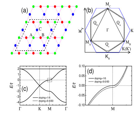
Figure 1: (a) Structure of the kagome lattice, made out of three sublattices $A$ (green dots), $B$ (red dots) and $C$ (blue dots). The dashed lines in the figure denote the enlarged unit cell in the $2\times 2$ charge density wave state. (b) Fermi surface produced by the Hamiltonian $H_{0}(\mathbf{k})$ for the doping levels $1/6$ (solid lines) and $9.6/60$ (dotted lines), respectively. (c) Tight-binding dispersion along high-symmetry cuts for doping levels 1/6 (solid curve) and 9.6/60 (dotted curve) (Note that the solid and dotted curves are close to each other, so only one solid curve can be discerned in a large energy scale). The dashed line denotes the Fermi level. (d) The enlarged view of the square box in (c).

Based on the Bogoliubov transformation, we obtain the following Bogoliubov-de Gennes equations in the EUC,

$$\sum_{\mathbf{k}\mathbf{\tilde{j}}}\left(\begin{array}[]{lr}H_{\mathbf{\tilde{i}\tilde{j}},\sigma}&\Delta_{\mathbf{\tilde{i}\tilde{j}}}\\ \Delta^{\ast}_{\mathbf{\tilde{i}\tilde{j}}}&-H^{\ast}_{\mathbf{\tilde{i}\tilde{j}},\bar{\sigma}}\end{array}\right)\exp[i\mathbf{k}\cdot(\textbf{r}_{\mathbf{\tilde{j}}}-\textbf{r}_{\mathbf{\tilde{i}}})]\left(\begin{array}[]{lr}u^{\mathbf{k}}_{n,\mathbf{\tilde{j}},\sigma}\\ v^{\mathbf{k}}_{n,\mathbf{\tilde{j}},\bar{\sigma}}\end{array}\right)$$ (17)

$$=E^{\mathbf{k}}_{n}\left(\begin{array}[]{lr}u^{\mathbf{k}}_{n,\mathbf{\tilde{i}},\sigma}\\ v^{\mathbf{k}}_{n,\mathbf{\tilde{i}},\bar{\sigma}}\end{array}\right),$$ (20)

where $H_{\mathbf{\tilde{i}}\mathbf{\tilde{j}},\sigma}=(-t+iW_{\mathbf{\tilde{i}\tilde{j}}})\delta_{\mathbf{\tilde{i}}+\mathbf{\tau}_{\mathbf{\tilde{j}}},\mathbf{\tilde{j}}}-\mu\delta_{\mathbf{\tilde{i}},\mathbf{\tilde{j}}}$ with $\mathbf{\tau}_{\mathbf{\tilde{j}}}$ denoting the four NN vectors and $\Delta_{\mathbf{\tilde{i}\tilde{j}}}=\Delta\delta_{\mathbf{\tilde{i}},\mathbf{\tilde{j}}}$. $u^{\mathbf{k}}_{n,\mathbf{\tilde{i}},\sigma}$ and $v^{\mathbf{k}}_{n,\mathbf{\tilde{i}},\bar{\sigma}}$ are the Bogoliubov quasiparticle amplitudes on the $\mathbf{\tilde{i}}$-th site with momentum $\mathbf{k}$ and eigenvalue $E^{\mathbf{k}}_{n}$. The amplitudes of the SC pairing and the orbital current order, as well as the electron densities, are obtained through the following self-consistent equations,

$$\Delta= \frac{V_{s}}{2}\sum_{\mathbf{k},n}u^{\mathbf{k}}_{n,\mathbf{\tilde{i}},\sigma}v^{\mathbf{k}\ast}_{n,\mathbf{\tilde{i}},\bar{\sigma}}\tanh(\frac{E^{\mathbf{k}}_{n}}{2k_{B}T})$$

$$W_{\mathbf{\tilde{i}}\mathbf{\tilde{j}}}= \frac{V_{c}}{2}\textmd{Im}\{\sum_{\mathbf{k},n}(u^{\mathbf{k}}_{n,\mathbf{\tilde{i}},\sigma}u^{\mathbf{k}\ast}_{n,\mathbf{\tilde{j}},\sigma}+v^{\mathbf{k}}_{n,\mathbf{\tilde{i}},\bar{\sigma}}v^{\mathbf{k}\ast}_{n,\mathbf{\tilde{j}},\bar{\sigma}})$$

$$\times\exp[-i\mathbf{k}\cdot(\textbf{r}_{\mathbf{\tilde{j}}}-\textbf{r}_{\mathbf{\tilde{i}}})]\tanh(\frac{E^{\mathbf{k}}_{n}}{2k_{B}T})\}$$

$$n_{\mathbf{\tilde{i}}}= \sum_{\mathbf{k},n}\{|u^{\mathbf{k}}_{n,\mathbf{\tilde{i}},\uparrow}|^{2}f(E^{\mathbf{k}}_{n})+|v^{\mathbf{k}}_{n,\mathbf{\tilde{i}},\downarrow}|^{2}[1-f(E^{\mathbf{k}}_{n})]\}.$$ (21)

Due to the fairly good FS nesting, the proximity to the VHF, and the presence of multiple electronical orders, the self-consistent calculations may yield several solutions with local energy minima at the same temperature and doping. In cases where multiple solutions arise from the self-consistent calculations at the same temperature but with different sets of initially random input parameters, we compare their free energy defined as

$$F= -2k_{B}T\sum_{\mathbf{k},n,E^{\mathbf{k}}_{n}>0}\ln[2\cosh(\frac{E^{\mathbf{k}}_{n}}{2k_{B}T})]+N\frac{|\Delta|^{2}}{V_{s}}$$ (22)

$$+\sum_{\mathbf{k},\langle\mathbf{\tilde{i}}\mathbf{\tilde{j}}\rangle}\frac{|W_{\mathbf{\tilde{i}}\mathbf{\tilde{j}}}|^{2}}{2V_{c}},$$

so as to find the most favorable state in energy.

Then, the single-particle Green’s functions $G_{\mathbf{\tilde{i}}\mathbf{\tilde{j}}}(\mathbf{k},i\omega)=-\int^{\beta}_{0}d\tau\exp^{i\omega\tau}\langle T_{\tau}c_{\mathbf{k}\mathbf{\tilde{i}}}(i\tau)c^{{\dagger}}_{\mathbf{k}\mathbf{\tilde{j}}}(0)\rangle$ can be expressed as

$$G_{\mathbf{\tilde{i}}\mathbf{\tilde{j}}}(\mathbf{k},i\omega)=\sum_{n}\left(\frac{u^{\mathbf{k}}_{n,\mathbf{\tilde{i}},\uparrow}u^{\mathbf{k}\ast}_{n,\mathbf{\tilde{j}},\uparrow}}{i\omega-E^{\mathbf{k}}_{n}}+\frac{v^{\mathbf{k}}_{n,\mathbf{\tilde{i}},\downarrow}v^{\mathbf{k}\ast}_{n,\mathbf{\tilde{j}},\downarrow}}{i\omega+E^{\mathbf{k}}_{n}}\right).$$ (23)

The spectral function $A(\mathbf{k},E)$ and the DOS $\rho(E)$ can be derived from the analytic continuation of the Green’s function as,

$$A(\mathbf{k},E)=-\frac{1}{N_{P}\pi}\sum_{\mathbf{\tilde{i}}}\textmd{Im}G_{\mathbf{\tilde{i}}\mathbf{\tilde{i}}}(\mathbf{k},iE\rightarrow E+i0^{+}),$$ (24)

and

$$\rho(E)=\frac{1}{N_{\mathbf{k}}}\sum_{\mathbf{k}}A(\mathbf{k},E),$$ (25)

where $N_{P}$ and $N_{\mathbf{k}}$ are the number of PUCs in the EUC and the number of $\mathbf{k}$-points in the Brillouin zone, respectively.

III Results and discussion

III.1 Phase Diagram

In the following analysis, the chemical potential $\mu$ is adjusted to achieve the desired filling. Right at the VHF, the FS possesses a hexagonal shape, with the saddle points $M_{A/B/C}$ located exactly on the FS. This unique FS possesses a perfect nesting property and facilitates the inter-scatterings between three van Hove singularities connected by the nesting vectors $\mathbf{Q}_{a}=(-\pi,\sqrt{3}\pi)$, $\mathbf{Q}_{b}=(-\pi,-\sqrt{3}\pi)$ and $\mathbf{Q}_{c}=(2\pi,0)$, which has been considered as the primary factors promoting the so-called “triple-$Q$” $2\times 2$ CDW in AV₃Sb₅ Ortiz1 ; YXJiang1 ; HZhao1 ; Liang1 ; HChen1 ; HLi2 ; Mielke1 . Away from the VHF, the FS becomes more rounded, and the nesting is weakened, particularly around the saddle points [$M_{A/B/C}$ in Fig. 1(b)]. We focus on the situation where the hole doping is deceased from $1/6$, such that the saddle points move slightly below the Fermi level as displayed in Figs. 1(c) and (d), being consistent with the density functional theory calculations TPark1 ; JZhao1 ; YLi1 ; HZhao1 .

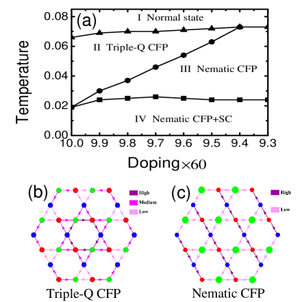
Figure 2: (a) Phase diagram as a function of doping and temperature. The orbital current configurations for the “triple-$Q$” CFP (b), and the nematic CFP (c), respectively. The arrows in (b) with their respective colors indicated by the labels of “High”, “Medium” and “Low” signal the magnitudes of the bond current orders. The arrows in (c) with their respective colors indicated by the labels of “High” and “Low” signal the magnitudes of the bond current orders. In (c), the large (green dots) and small (red and blue dots) sizes of lattice site also signal respectively the “High” and “Low” values of the on-site SC pairing amplitude in the coexisting phase(see text and Table II for reference).

As a function of doping and temperature, we find a rich phase diagram of the model at and near the VHF, which is summarized in Fig. 2(a) for the typical values of $V_{s}=1.4$ and $V_{c}=1.2$. Right at the VHF for $1/6$ doping, where the DOS at the Fermi level is maximally enhanced and the nesting features of the FS are strongest, the system prefers the TCFP [Fig. 2(b)] before entering the SC state. Once the system deviates from the VHF, the NCFP order [Fig. 2(c)] develops in between the TCFP and the low-temperature SC state. In this case, when decreasing the temperature, the system starts from the high-temperature normal state and passes through the NCFP state, and finally transits into the SC state. When the filling further departs from the van Hove point, the region of the NCFP expands gradually towards higher temperatures with the concomitant shrinking of the TCFP region, and eventually the TCFP is completely displaced by the NCFP state. Interestingly, the SC state always coexists with the NCFP state in the low temperature region of the phase diagram, with its free energy being significantly lower than those of the pure states. Although the variations of $V_{s}$ and $V_{c}$ may affect the phase boundaries, the essential feature of the phase diagram, namely the consecutive evolvement of different ordered states with temperature, remains qualitatively unchanged.

It is remarkable that the successive temperature evolutions from the TCFP phase to the NCFP state, occurring at a doping level slightly deviating from the van Hove point in a self-consistent manner, exhibits the same trend as the experimental observations HLi1 ; ZJiang1 ; LNie1 ; PWu1 . Particularly, the ground state characterized by the coexistence of the NCFP and SC orders may be related to the $C_{2}$ symmetry and the time-reversal-symmetry breaking observed in the SC state Xiang1 ; HZhao1 ; HLi1 .

Since the effect of doping on the phase diagram is closely related to the VHF, we will focus on the physics associated with the three van Hove points, in addition to the nesting properties of the FS. At each van Hove point, the electronic states come exclusively from one of the three distinct sublattices SLYu1 . As a result, the scattering between low-energy electronic states connected by each nesting wave vector occurs solely between two sublattices. This unique property creates the necessary conditions for the transition from the TCFP to the NCFP through doping. At VHF, the electronic states at the three van Hove points are mutually coupled by the CDW orders with three wave vectors $\mathbf{Q}_{a}$, $\mathbf{Q}_{b}$ and $\mathbf{Q}_{c}$ in the TCFP in an end-to-end manner [Fig. 1(b)]. This is to say, the CDW orders with three wave vectors are mutually coupled in pairs with the strongest coupling strength at the van Hove points. Thus, as depicted in the phase diagram [Fig. 2(a)], a stable charge order pattern that simultaneously satisfies the three wave vectors can be found at the VHF. However, when the system deviates from the VHF by reducing the hole doping, the chemical potential $\mu$ is elevated, and accordingly the saddle points move below the Fermi level, as demonstrated in Figs. 1(c) and (d). The deviation of the FS from the saddle points weakens the mutual couplings between pairs of the three wave vectors and, correspondingly, the TCFP. In this situation, there is a significant decrease in the energy difference between the TCFP, which satisfies three ordered wave vectors, and the NCFP, which has only one ordered wave vector. Moreover, the NCFP will deform the FS, suppressing the other two NCFP with different ordered wave vectors while further enhancing itself [refer to Fig. 2(c) and Table I]. Consequently, within a certain doping range, the NCFP becomes more stable than the TCFP. For better clarity, we present the evolutions of the free energy deference between the TCFP and the NCFP with doping at a specific temperature $T=0.04$ in Fig. 3(a). It shows that the TCFP has a lower free energy than that of the NCFP, when the doping level has not much deviations from the VHF. Nevertheless, as the system deviates appreciably from the VHF, the NCFP acquires the lower free energy. As a result, a spontaneous rotational symmetry-breaking transition occurs from the TCFP to the NCFP at the doping level defined by the zero point of the free energy difference.

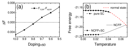
Figure 3: (a) Doping dependence of the free energy difference per site between the “triple-$Q$” CFP and nematic CFP. In obtaining the results in (a), the CDW states are each intentionally kept in their respective forms during the calculations. (b) The evolutions of the free energy per site from the normal state (dashed line) to pure SC state (dashed ling with square symbol), and from the nematic CFP (dotted line) to the coexisting phase with nematic CFP and SC state (dotted line with round symbol) at doping level $9.8/60$.

The temperature effects on the CDW states are also closely related to the van Hove physics. Although the van Hove points shift below the Fermi level for doping levels deviating from the VHF, the thermal broadening effect becomes prominent at relatively high temperatures, thereby increasing the effectiveness of the van Hove points. This enhances the mutual coupling among three CDW orders associated with different wave vectors $\mathbf{Q}_{a}$, $\mathbf{Q}_{b}$ and $\mathbf{Q}_{c}$. As a result, for doping levels that deviate from the VHF, the TCFP is stabilized by the thermal broadening effect at relatively high temperatures, while the NCFP becomes more favorable due to the reduction of thermal broadening effect at low temperatures.

Previously, the transition to the CDW with $C_{2}$ symmetry was proposed to arise from interlayer interactions between adjacent kagome planes with already existing $C_{6}$-symmetry charge orders in each single layer TPark1 ; Christ1 . As a secondary outcome of the $C_{6}$-symmetry charge orders in this interlayer coupling scenario, the nematicity typically occurs at a lower temperature $T_{nem}$ well below $T_{CDW}$. However, as shown in Fig. 2(a), our theory shows a regime of less than $9.4/60$ hole doping where the NCFP directly straddles the normal and SC states, despite in the high doping level regime of the phase diagram the appearance of nematic CDW at low temperatures is well below $T_{CDW}$. Interestingly, a recent experiment has indeed observed an immediate development of nematicity and possible time-reversal symmetry breaking in the CDW state of CsV₃Sb₅ QWu1 , providing further support on our theory.

As the temperature continues to decrease, several ingredients promote the development of the coexisting phase of the NCFP and SC state. First of all, as depicted in Figs. 3(b) and  A1(a), the NCFP exhibits a lower energy compared to the normal and TCFP states before the SC transition, making it energetically favorable as the parent state for the formation of the SC order. Secondly, the well-preserved portions of the FS, especially those portions near the saddle points [the $M_{A}$ points in Fig 4(b)], within the NCFP provide sufficient electronic states for the formation of the SC pairing. Thirdly, apart from the gaped portions of the FS, the one-wave-vector scattering with the rotational symmetry breaking in the NCFP state induces a slight deformation of the FS [refer to Figs. 4(b) and  A1(b)], which brings the remaining FS closer to the van Hove points compared to the normal state. As a result, the coexisting phase of NCFP and SC orders possesses the significantly lower free energy than that for the pure SC state [see Fig. 3(b)].

III.2 Characteristics of electronic states

Next, we will investigate in detail on the electronic structures in different regime of the phase diagram, namely the TCFP state, the NCFP state, and the coexisting state of the NCFP and SC orders. To demonstrate our results, we will focus on the typical cases with a doping level of $9.8/60$ at temperatures $T=0.05$, $T=0.03$ and $T=1\times 10^{-5}$, corresponding to the TCFP state, the NCFP state and the coexisting phase of the NCFP and SC orders, respectively.

For the TCFP, the bond current orders obtained from self-consistent calculations can be classified into three levels of magnitude: “High”, “Medium” and “Low”, as displayed in Fig. 2(b) and listed in Table I. These orders give rise to a special pattern known as the “Star of David” state. Fig. 4(a) presents the distribution of spectral weight $A(\mathbf{k},E)$ at $E=0$, which is unfolded in the primitive Brillouin zone. Consistent with the previous non-self-consistent results HMJiang2 , the zero-energy spectral weight distribution clearly reveals partially gapped Fermi segments and preserves the $C_{6}$ symmetry. Correspondingly, the DOS shown in Fig. 5(a) exhibits a “pseudogap-like” feature, with non-zero minima occurring at $E=0$. In contrast, the DOS for the normal state, represented by the black dashed curve in the same figure, displays the typical van Hove peak near $E=0$.

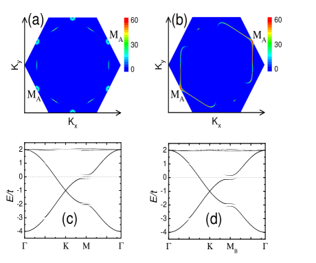
Figure 4: Zero-energy spectral weight distribution $A(\mathbf{k},E)$ unfolded in the primitive Brillouin zone for hole doping $9.8/60$ at $T=0.05$ (a), and at $T=0.03$ (b), respectively. The former situates in the “triple-$Q$” CFP region, while the latter lies in the region of the nematic CFP state. The unfolded dispersions along high-symmetry cuts in the primitive Brillouin zone are shown correspondingly in (c) for the “triple-$Q$” CFP state, and in (d) for the nematic CFP state, respectively.

On the other hand, as the temperature decreases into the NCFP regime, such as $T=0.03$, the magnitude distribution of the three inequivalent bond current orders transforms into that of two inequivalent orders. The “Low” intensity is associated with two inequivalent bonds, which are approximately one order of magnitude smaller than the other one labeled as “High” intensity. In this case, only the strong current order between sublattices $B$ and $C$ corresponds to the charge order scattering between $M_{B}$ and $M_{C}$ points with a momentum transfer $\mathbf{Q}_{a}$. As a result, the depletion of the zero-energy spectral weight only occurs in regions connected by one of the three wave vectors, such as $\mathbf{Q}_{a}$ in Fig. 4(b), manifesting the characteristics of the $C_{2}$ symmetry. The DOS for the NCFP depicted by the black solid curve in Fig. 5(b) still exhibits two peaks resembling gap edges, but a significant DOS shows up within the peak edges, accompanied by a residue van Hove peak near the zero bias, resulting from the large portion of the unspoilt Fermi segments and the preserved van Hove points $M_{A}$.

	High	Medium	Low
“triple-$Q$” CFP	0.043805	0.035128	0.026666
nematic CFP	0.071768		0.00841

Table 1: Magnitude of the bond current order $|W_{ij}|$ in the self-consistent calculations at filling level $9.8/60$ with $T=0.05$ for the “triple-$Q$” CFP and $T=0.03$ for the nematic CFP.

Let’s further analyze the characteristics of the band structures in the two CDW states. In the TCFP, the bands along different high-symmetry cuts $\Gamma\rightarrow K/K^{\prime}\rightarrow M_{A/B/C}\rightarrow\Gamma$ remain the same due to the preservation of the $C_{6}$ symmetry, while in the NCFP, a gap opens near the $M_{B/C}$ points but not near the $M_{A}$ point, as shown in Figs. 4(d),  A2(a) and  A2(b). In addition, near the saddle point, the band is triply split in the TCFP, while it is only double split near the $M_{B/C}$ points in the NCFP, as illustrated in Figs. 4(c), (d) and Fig.  A2(a). This behavior can be understood through the “patch model”, which provides an approximate description of the low-energy scatterings between the saddle points Nand1 ; YPLin1 ; YPLin2 . In the TCFP state, the patch model involving the “triple-$Q$” scatterings reads,

$$H_{TCFP}(M)=\left(\begin{array}[]{ccc}\varepsilon_{M_{A}}&i\lambda_{AB}&i\lambda_{AC}\\ -i\lambda_{AB}&\varepsilon_{M_{B}}&i\lambda_{BC}\\ -i\lambda_{AC}&-i\lambda_{BC}&\varepsilon_{M_{C}}\end{array}\right).$$ (29)

Nevertheless, the charge order scattering in the NCFP involves only one wave vector, such as $\mathbf{Q}_{a}$ that corresponds to the bond current configuration in Fig. 2(c). As a result, the patch model in the NCFP state is reduced to

$$H_{NCFP}(M)=\left(\begin{array}[]{cc}\varepsilon_{M_{B}}&i\lambda_{BC}\\ -i\lambda_{BC}&\varepsilon_{M_{C}}\end{array}\right).$$ (32)

Here, $\varepsilon_{M_{A}}$ ($\varepsilon_{M_{B}}$, $\varepsilon_{M_{C}}$) stands for the energy at the saddle point $M_{A}$ ($M_{B}$, $M_{C}$) that originates from the sublattice $A$ ($B$, $C$), and $\lambda_{AB}$ ($\lambda_{AC}$, $\lambda_{BC}$) represents the scattering strength of the bond current order between $M_{A}$ and $M_{B}$ ($M_{A}$ and $M_{C}$, $M_{B}$ and $M_{C}$). Near the VHF, where $\varepsilon_{M_{A}}=\varepsilon_{M_{B}}=\varepsilon_{M_{C}}\approx 0$, one can immediately find that the Hamiltonian $H_{TCFP}(M)$ has three eigenvalues $E_{0}(M)=0$ and $E_{\pm}(M)=\pm\sqrt{\lambda_{AB}^{2}+\lambda_{AC}^{2}+\lambda_{BC}^{2}}$. The Hamiltonian $H_{NCFP}(M)$, on the other hand, has two eigenvalues $E_{\pm}(M)=\pm|\lambda_{BC}|$. It is worth pointing out that the unique change of the electronic structures from the TCFP to the NCFP can serve as an indirect evidence to identify the electronic nematicity in AV₃Sb₅.

	High	Low
nematic CFP	0.072113	0.008144
SC	0.050711	0.025567

Table 2: Magnitudes of the bond current order $|W_{ij}|$ and the SC pairing $|\Delta|$ in the self-consistent calculations at filling level $9.8/60$ with $T=1\times 10^{-5}$ for the coexisting phase of the nematic CFP and SC orders.

Then, we turn to the coexisting phase of the NCFP and SC orders. On the one hand, as indicated in Table II, the strength of the bond current orders changes little upon entering the coexisting phase. On the other hand, as displayed in Fig. 2(c), the distribution of SC pairing amplitudes depends not only on the strength but also on the direction of the surrounding bond current orders. Specifically, the “High” value of the SC pairing amplitude appears at the sublattice site [the sublattice $A$ in Fig. 2(c)] where the surrounding bond current orders are weak and the bonds connected to the same sublattice sites carry either the same inflow current directions or the same outflow current directions. On the contrary, the “Low” value of the SC pairing amplitude appears on the sublattice sites where a pair of bonds connected to the same sublattice sites have respective inflow and outflow current directions. The uneven distribution of the SC pairing amplitude can be understood from the low energy spectral distribution shown in Fig. 4(b). In the coexisting phase of the NCFP and SC orders, since the depletion of the low energy spectral weight only occurs at portions between $M_{B}$ and $M_{C}$, the remained spectral weights, including the perfect van Hove points $M_{A}$ caused by the deformation of the FS, mainly come from the sublattice $A$. Consequently, the SC pairing amplitude on sublattice $A$ is significantly larger than those on the sublattices $B$ and $C$.

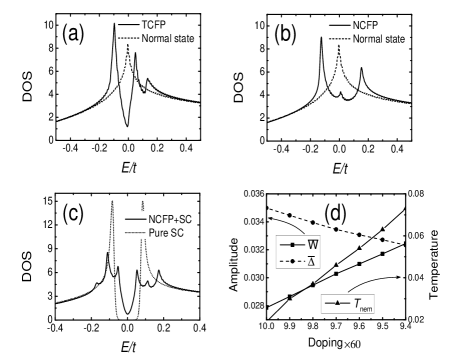
Figure 5: Energy dependence of the DOSs for the “triple-$Q$” CFP (a), the nematic CFP (b), and the coexisting phase of the nematic CFP and SC orders (c), respectively. (d) The doping dependence of the averaged SC pairing amplitude $\bar{\Delta}$, the averaged magnitude of the bond current orders $\bar{W}$, and the transition temperature of the nematic CFP $T_{nem}$.

Due to the uneven distributions of the SC pairing amplitude and the scattering of the CDW order, a V-shaped DOS can be observed in Fig. 5(c), accompanied by multiple sets of coherent peaks and residual zero-energy DOS, constituting a characteristic of a nodal multi-gap SC pairing state as having been observed in the STM experiments HSXu1 ; Liang1 ; HChen1 . For comparison, the dotted curve in the same figure portrays a typical U-shaped full gap structure for the DOS in the state with pure on-site $s$-wave SC pairing.

Considering the nature of the mean-field approximation, it should be noted that the transition temperature between different phases in the calculated results is just qualitative rather than quantitative. Nevertheless, the anti-correlation trend between the SC pairing amplitude and the transition temperature of the nematic phase at different doping levels can be clearly observed in Fig. 5(d), as supported by the STM experiments PWu1 .

IV Conclusion

In conclusion, we have investigated the origin of the chiral CDW and its interplay with superconductivity in a fully self-consistent theory considering the orbital current order and the on-site SC pairing, which determines both the CDW and the SC orders self-consistently. It was revealed that the self-consistent theory captures the salient feature for the successive temperature evolutions of the ordered electronic states from the high-temperature $2\times 2$ TCFP to the NCFP, and to the low-temperature $s$-wave SC state in a coexisting manner with the NCFP order. The rotational symmetry breaking transition of the CDW could be understood from a scenario in which the competition between the deviation from the VHF and the thermal broadening of the FS determines which state is it in. The intertwining of the $s$-wave SC pairing with the NCFP order produced a nodal gap feature manifesting as the V-shaped DOS along with the residual DOS near the Fermi energy. The self-consistent theory not only produced the successive temperature evolutions of the electronically ordered states observed in experiment, but might also offer a heuristic explanation to the two-fold rotational symmetry of electron state detected in both the CDW and the SC states. Moreover, the intertwining of the SC pairing with the NCFP order, which was found to be a ground state in the self-consistent theory at the low temperature regime, might also be a promising alternative for mediating the divergent or seemingly contradictory experimental outcomes regarding the SC properties. Overall, our study sheds light on the intricate relationship between the chiral CDW and superconductivity, providing valuable insights into the underlying mechanisms and experimental observations.

V acknowledgement

This work was supported by National Key Projects for Research and Development of China (Grant No. 2021YFA1400400), and the National Natural Science Foundation of China (Grants No. 12074175, No. 12374137 and No. 92165205).

*

Appendix A Temperature evolution of free energy, details of spectrum and band structures along high-symmetry cuts

In Fig. A1(a), we show the temperature evolution of the free energy in the TCFP and in the NCFP. In Fig. A1(b), we display the momentum cut of the spectral weight along the $M_{A}\rightarrow\Gamma\rightarrow M_{A}$ direction [see Fig. 4(b) in the main text] at a doping level deviating from the VHF for the normal state and for the NCFP.

Figure A1: (a) Temperature evolution of the free energy per site for the doping level $9.8/60$ in the “triple-$Q$” CFP (solid line) and in the nematic CFP (dotted line). In obtaining the results in (a), the CDW states are intentionally kept in their respective forms during the calculations. (b) The momentum cut of the spectral weight along the $M_{A}\rightarrow\Gamma\rightarrow M_{A}$ direction at a doping level deviating from the VHF for the normal state (solid curve) and for the nematic CFP (dotted curve). The peaks of the spectral weight intensity denote the position of the Fermi surface [refer to Fig. 4(b) in the main text]. The same figure of (b) is replotted in the inset by breaking the $x$-axis in order to have a better view of the Fermi surface shift.

In Fig. A2, we present the unfolded dispersions of the spectral weight along different high-symmetry cuts for the NCFP. Owing to the $C_{2}$ symmetry of the NCFP, the energy bands exhibit different features along different high symmetry cut. Specifically, an energy gap opens near the $M_{B/C}$ points but not near the $M_{A}$ point, as presented respectively in Figs. A2(a) and (b).

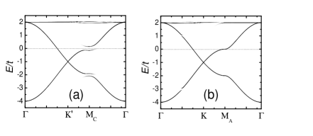
Figure A2: The unfolded dispersions along high-symmetry cuts $\Gamma$-$K^{\prime}$-$M_{C}$-$\Gamma$ (a), and $\Gamma$-$K$-$M_{A}$-$\Gamma$ (b), respectively.

References

- (1) Y. Ran, M. Hermele, P. A. Lee, and X.-G. Wen, Phys. Rev. Lett. 98, 117205 (2007).
- (2) H. C. Jiang, Z. Y. Weng, and D. N. Sheng, Phys. Rev. Lett. 101, 117203 (2008).
- (3) S. Yan, D. A. Huse, and S. R. White, Science 332, 1173 (2011).
- (4) S. Depenbrock, I. P. McCulloch, and U. Schollwöck, Phys. Rev. Lett. 109, 067201 (2012).
- (5) T.-H. Han, J. S. Helton, S. Chu, D. G. Nocera, J. A. Rodriguez-Rivera, C. Broholm, and Y. S. Lee, Nature 492, 406 (2012).
- (6) Y.-C. He, D. N. Sheng, and Y. Chen, Phys. Rev. Lett. 112, 137202 (2014).
- (7) H. J. Liao, Z. Y. Xie, J. Chen, Z. Y. Liu, H. D. Xie, R. Z. Huang, B. Normand, and T. Xiang, Phys. Rev. Lett. 118, 137202 (2017).
- (8) Zili Feng, Zheng Li, Xin Meng, Wei Yi, Yuan Wei, Jun Zhang, Yan-Cheng Wang, Wei Jiang, Zheng Liu, Shiyan Li, Feng Liu, Jianlin Luo, Shiliang Li, Guo-qing Zheng, Zi Yang Meng, Jia-Wei Mei, and Youguo Shi, Chin. Phys. Lett. 34, 077502 (2017).
- (9) P. Khuntia, M. Velazquez, Q. Barth¨¦lemy, F. Bert, E. Kermarrec, A. Legros, B. Bernu, L. Messio, A. Zorko, and P. Mendels, Nat. Phys. 16, 469 (2020).
- (10) H.-M. Guo and M. Franz, Phys. Rev. B 80, 113102 (2009).
- (11) S.-L. Yu, J.-X. Li, and L. Sheng, Phys. Rev. B 80, 193304 (2009).
- (12) J. Wen, A. Rüegg, C.-C. Joseph Wang, and G. A. Fiete, Phys. Rev. B 82, 075125 (2010).
- (13) E. Tang, J.-W. Mei, and X.-G. Wen, Phys. Rev. Lett. 106, 236802 (2011).
- (14) G. Xu, B. Lian, and S.-C. Zhang, Phys. Rev. Lett. 115, 186802 (2015).
- (15) L. Ye, M. Kang, J. Liu, F. v. Cube, C. R. Wicker, T. Suzuki, C. Jozwiak, A. Bostwick, E. Rotenberg, D. C. Bell, L. Fu, R. Comin. and J. G. Checkelsky, Nature 555, 638 (2018).
- (16) D. F. Liu, A. J. Liang, E. K. Liu, Q. N. Xu, Y. W. Li, C. Chen, D. Pei, W. J. Shi, S. K. Mo, P. Dudin, T. Kim, C. Cacho, G. Li, Y. Sun, L. X. Yang, Z. K. Liu, S. S. P. Parkin, C. Felser, and Y. L. Chen, Science 365, 1282 (2019).
- (17) J.-X. Yin, W. Ma, T. A. Cochran, X. Xu, S. S. Zhang, H.-J. Tien, N. Shumiya, G. Cheng, K. Jiang, B. Lian, Z. Song, G. Chang, I. Belopolski, D. Multer, M. Litskevich, Z.-J. Cheng, X. P. Yang, B. Swidler, H. Zhou, H. Lin, T. Neupert, Z. Wang, N. Yao, T.-R. Chang, S. Jia, and M. Z. Hasan, Nature 583, 533 (2020).
- (18) A. Rüegg and G. A. Fiete, Phys. Rev. B 83, 165118 (2011).
- (19) S.-L. Yu and J.-X. Li, Phys. Rev. B 85, 144402 (2012).
- (20) S. V. Isakov, S. Wessel, R. G. Melko, K. Sengupta, and Y. B. Kim, Phys. Rev. Lett. 97, 147202 (2006).
- (21) M. L. Kiesel, C. Platt, and R. Thomale, Phys. Rev. Lett. 110, 126405 (2013).
- (22) W.-S. Wang, Z.-Z. Li, Y.-Y. Xiang, and Q.-H. Wang, Phys. Rev. B 87, 115135 (2013).
- (23) W.-H. Ko, P. A. Lee, and X.-G. Wen, Phys. Rev. B 79, 214502 (2009).
- (24) J. Kang, S.-L. Yu, Z.-J. Yao, and J.-X. Li, J. Phys.: Condens. Matter 23, 175702 (2011).
- (25) B. R. Ortiz, S. M. L. Teicher, Y. Hu, J. L. Zuo, P. M. Sarte, E. C. Schueller, A. M. M. Abeykoon, M. J. Krogstad, S. Rosenkranz, R. Osborn, R. Seshadri, L. Balents, J. He, and S. D. Wilson, Phys. Rev. Lett. 125, 247002 (2020).
- (26) Y.-X. Jiang, J.-X. Yin, M. M. Denner, N. Shumiya, B. R. Ortiz, G. Xu, Z. Guguchia, J. He, M. S. Hossain, X. Liu, J. Ruff, L. Kautzsch, S. S. Zhang, G. Chang, I. Belopolski, Q. Zhang, T. A. Cochran, D. Multer, M. Litskevich, Z.-J. Cheng, X. P. Yang, Z. Wang, R. Thomale, T. Neupert, S. D. Wilson, and M. Z. Hasan, Nat. Mater. 20, 1353 (2021).
- (27) H. Zhao, H. Li, B. R. Ortiz, S. M. L. Teicher, T. Park, M. Ye, Z. Wang, L. Balents, S. D. Wilson, and I. Zeljkovic, Nature 599, 216 (2021).
- (28) H. Chen, H. Yang, B. Hu, Z. Zhao, J. Yuan, Y. Xing, G. Qian, Z. Huang, G. Li, Y. Ye, S. Ma, S. Ni, H. Zhang, Q. Yin, C. Gong, Z. Tu, H. Lei, H. Tan, S. Zhou, C. Shen, X. Dong, B. Yan, Z. Wang, and H.-J. Gao, Nature 599, 222 (2021).
- (29) Z. Liang, X. Hou, F. Zhang, W. Ma, P. Wu, Z. Zhang, F. Yu, J.-J. Ying, K. Jiang, L. Shan, Z. Wang, and X.-H. Chen, Phys. Rev. X 11, 031026 (2021).
- (30) H. Li, T. T. Zhang, T. Yilmaz, Y. Y. Pai, C. E. Marvinney, A. Said, Q. W. Yin, C. S. Gong, Z. J. Tu, E. Vescovo, C. S. Nelson, R. G. Moore, S. Murakami, H. C. Lei, H. N. Lee, B. J. Lawrie, and H. Miao, Phys. Rev. X 11, 031050 (2021).
- (31) C. Mielke III, D. Das, J.-X. Yin, H. Liu, R. Gupta, Y.-X. Jiang, M. Medarde, X. Wu, H. C. Lei, J. Chang, P. Dai, Q. Si, H. Miao, R. Thomale, T. Neupert, Y. Shi, R. Khasanov, M. Z. Hasan, H. Luetkens, and Z. Guguchia, Nature 602, 245 (2022).
- (32) F. H. Yu, T. Wu, Z. Y. Wang, B. Lei, W. Z. Zhuo, J. J. Ying, and X. H. Chen, Phys. Rev. B 104, L041103 (2021).
- (33) N. Shumiya, Md. S. Hossain, J.-X. Yin, Y.-X. Jiang, B. R. Ortiz, H. Liu, Y. Shi, Q. Yin, H. Lei, S. S. Zhang, G. Chang, Q. Zhang, T. A. Cochran, D. Multer, M. Litskevich, Z.-J. Cheng, X. P. Yang, Z. Guguchia, S. D. Wilson, and M. Z. Hasan, Phys. Rev. B 104, 035131 (2021).
- (34) C. Guo, C. Putzke, S. Konyzheva, X. Huang, M. Gutierrez-Amigo, I. Errea, D. Chen, M. G. Vergniory, C. Felser, M. H. Fischer, T. Neupert, and P. J. W. Moll, Nature 611, 461 (2022).
- (35) S.-Y. Yang, Y. Wang, B. R. Ortiz, D. Liu, J. Gayles, E. Derunova, R. Gonzalez-Hernandez, L. Šmejkal, Y. Chen, S. S. P. Parkin, S. D. Wilson, E. S. Toberer, T. McQueen, and M. N. Ali, Sci. Adv. 6, eabb6003 (2020).
- (36) B. R. Ortiz, P. M. Sarte, E. M. Kenney, M. J. Graf, S. M. L. Teicher, R. Seshadri, and S. D. Wilson, Phys. Rev. Mater. 5, 034801 (2021).
- (37) Q. Yin, Z. Tu, C. Gong, Y. Fu, S. Yan, and H. Lei, Chin. Phys. Lett. 38, 037403 (2021).
- (38) K. Y. Chen, N. N. Wang, Q. W. Yin, Y. H. Gu, K. Jiang, Z. J. Tu, C. S. Gong, Y. Uwatoko, J. P. Sun, H. C. Lei, J. P. Hu, and J.-G. Cheng, Phys. Rev. Lett. 126, 247001 (2021).
- (39) Y. Wang, S. Yang, P. K. Sivakumar, B. R. Ortiz, S. M. L. Teicher, H. Wu, A. K. Srivastava, C. Garg, D. Liu, S. S. P. Parkin, E. S. Toberer, T. McQueen, S. D. Wilson, and M. N. Ali, arXiv:2012.05898.
- (40) Z. Zhang, Z. Chen, Y. Zhou, Y. Yuan, S. Wang, J. Wang, H. Yang, C. An, L. Zhang, X. Zhu, Y. Zhou, X. Chen, J. Zhou, and Z. Yang, Phys. Rev. B 103, 224513 (2021).
- (41) X. Chen, X. Zhan, X. Wang, J. Deng, X.-B. Liu, X. Chen, J.-G. Guo, and X. Chen, Chin. Phys. Lett. 38, 057402 (2021).
- (42) H.-S. Xu, Y.-J. Yan, R. Yin, W. Xia, S. Fang, Z. Chen, Y. Li, W. Yang, Y. Guo, and D.-L. Feng, Phys. Rev. Lett. 127, 187004 (2021).
- (43) C. Mu, Q. Yin, Z. Tu, C. Gong, H. Lei, Z. Li, and J. Luo, Chin. Phys. Lett. 38, 077402 (2021).
- (44) W. Duan, Z. Nie, S. Luo, F. Yu, B. R. Ortiz, L. Yin, H. Su, F. Du, A. Wang, Y. Chen, X. Lu, J. Ying, S. D. Wilson, X. Chen, Y. Song, and H. Yuan, Sci. China-Phys. Mech. Astron. 64, 107462 (2021).
- (45) C. C. Zhao, L. S. Wang, W. Xia, Q. W. Yin, J. M. Ni, Y. Y. Huang, C. P. Tu, Z. C. Tao, Z. J. Tu, C. S. Gong, H. C. Lei, Y. F. Guo, X. F. Yang, and S. Y. Li, arXiv: 2102.08356.
- (46) S. Ni, S. Ma, Y. Zhang, J. Yuan, H. Yang, Z. Lu, N. Wang, J. Sun, Z. Zhao, D. Li, S. Liu, H. Zhang, H. Chen, K. Jin, J. Cheng, L. Yu, F. Zhou, X. Dong, J. Hu, H.-J. Gao, and Z. Zhao, Chin. Phys. Lett. 38, 057403 (2021).
- (47) Y. Xiang, Q. Li, Y. Li, W. Xie, H. Yang, Z. Wang, Y. Yao, and H.-H. Wen, Nat. Commun. 12, 6727 (2021).
- (48) B. R. Ortiz, S. M. L. Teicher, L. Kautzsch, P. M. Sarte, N. Ratcliff, J. Harter, J. P. C. Ruff, R. Seshadri, and S. D. Wilson, Phys. Rev. X 11, 041030 (2021).
- (49) X. Zhou, Y. Li, X. Fan, J. Hao, Y. Dai, Z. Wang, Y. Yao, and H.-H. Wen, Phys. Rev. B 104, L041101 (2021).
- (50) Z. Liu, N. Zhao, Q. Yin, C. Gong, Z. Tu, M. Li, W. Song, Z. Liu, D. Shen, Y. Huang, K. Liu, H. Lei, and S. Wang, Phys. Rev. X 11, 041010 (2021).
- (51) M. Kang, S. Fang, J.-K. Kim, B. R. Ortiz, S. H. Ryu, J. Kim, J. Yoo, G. Sangiovanni, D. D. Sante, B.-G. Park, C. Jozwiak, A. Bostwick, E. Rotenberg, E. Kaxiras, S. D. Wilson, J.-H. Park, and R. Comin, Nat. Phys. 18, 301 (2022).
- (52) Y. Fu, N. Zhao, Z. Chen, Q. Yin, Z. Tu, C. Gong, C. Xi, X. Zhu, Y. Sun, K. Liu, and H. Lei, Phys. Rev. Lett. 127, 207002 (2021).
- (53) Y. Song, T. Ying, X. Chen, X. Han, X. Wu, A. P. Schnyder, Y. Huang, J.-g. Guo, and X. Chen, Phys. Rev. Lett. 127, 237001 (2021).
- (54) H. Tan, Y. Liu, Z. Wang, and B. Yan, Phys. Rev. Lett. 127, 046401 (2021).
- (55) F. H. Yu, D. H. Ma, W. Z. Zhuo, S. Q. Liu, X. K. Wen, B. Lei, J. J. Ying, and X. H. Chen, Nat. Commun. 12, 3645 (2021).
- (56) L. Yin, D. Zhang, C. Chen, G. Ye, F. Yu, B. R. Ortiz, S. Luo, W. Duan, H. Su, J. Ying, S. D. Wilson, X. Chen, H. Yuan, Y. Song, and X. Lu, Phys. Rev. B 104, 174507 (2021).
- (57) K. Nakayama, Y. Li, T. Kato, M. Liu, Z. Wang, T. Takahashi, Y. Yao, and T. Sato, Phys. Rev. B 104, L161112 (2021).
- (58) K. Jiang, T. Wu, J.-X. Yin, Z. Wang, M. Z. Hasan, S. D. Wilson, X. Chen, and J. Hu, arXiv: 2109.10809.
- (59) L. Nie, K. Sun, W. Ma, D. Song, L. Zheng, Z. Liang, P. Wu, F. Yu, J. Li, M. Shan, D. Zhao, S. Li, B. Kang, Z. Wu, Y. Zhou, K. Liu, Z. Xiang, J. Ying, Z. Wang, T. Wu, and X. Chen, Nature 604, 59 (2022).
- (60) H. Luo, Q. Gao, H. Liu, Y. Gu, D. Wu, C. Yi, J. Jia, S. Wu, X. Luo, Y. Xu, L. Zhao, Q. Wang, H. Mao, G. Liu, Z. Zhu, Y. Shi, K. Jiang, J. Hu, Z. Xu, and X. J. Zhou, Nat. Commun. 13, 273 (2022).
- (61) T. Neupert, M. M. Denner, J.-X. Yin, R. Thomale, and M. Z. Hasan, Nat. Phys. 18, 137 (2022).
- (62) K. Nakayama, Y. Li, T. Kato, M. Liu, Z. Wang, T. Takahashi, Y. Yao, and T. Sato, Phys. Rev. X 12, 011001 (2022).
- (63) H. Li, S. Wan, H. Li, Q. Li, Q. Gu, H. Yang, Y. Li, Z. Wang, Y. Yao, and H.-H. Wen, Phys. Rev. B 105, 045102 (2022).
- (64) H. Li, H. Zhao, B. R. Ortiz, Y. Oey, Z. Wang, S. D. Wilson, and I. Zeljkovic, Nat. Phys. 19, 637 (2023).
- (65) X. Wu, T. Schwemmer, T. Müller, A. Consiglio, G. Sangiovanni, D. Di Sante, Y. Iqbal, W. Hanke, A. P. Schnyder, M. M. Denner, M. H. Fischer, T. Neupert, and R. Thomale, Phys. Rev. Lett. 127, 177001 (2021).
- (66) M. M. Denner, R. Thomale, and T. Neupert, Phys. Rev. Lett. 127, 217601 (2021).
- (67) S. Cho, H. Ma, W. Xia, Y. Yang, Z. Liu, Z. Huang, Z. Jiang, X. Lu, J. Liu, Z. Liu, J. Li, J. Wang, Y. Liu, J. Jia, Y. Guo, J. Liu, and D. Shen, Phys. Rev. Lett. 127, 236401 (2021).
- (68) Y.-P. Lin and R. M. Nandkishore, Phys. Rev. B 106, L060507 (2022).
- (69) L. Zheng, Z. Wu, Y. Yang, L. Nie, M. Shan, K. Sun, D. Song, F. Yu, J. Li, D. Zhao, S. Li, B. Kang, Y. Zhou, K. Liu, Z. Xiang, J. Ying, Z. Wang, T. Wu, and X. Chen, Nature 611, 682 (2022).
- (70) C. Wen, X. Zhu, Z. Xiao, N. Hao, R. Mondaini, H.-M. Guo, and S. Feng, Phys. Rev. B 105, 075118 (2022).
- (71) R. Tazai, Y. Yamakawa, S. Onari, and H. Kontani, Sci. Adv. 8, eabl4108 (2022).
- (72) H.-M. Jiang, S.-L. Yu, and X.-Y. Pan, Phys. Rev. B 106, 014501 (2022).
- (73) Z. Liu, N. Zhao, Q. Yin, C. Gong, Z. Tu, M. Li, W. Song, Z. Liu, D. Shen, Y. Huang, K. Liu, H. Lei, and S. Wang, Phys. Rev. X 11, 041010 (2021).
- (74) B. R. Ortiz, L. C. Gomes, J. R. Morey, M. Winiarski, M. Bordelon, J. S. Mangum, I. W. H. Oswald, J. A. Rodriguez-Rivera, J. R. Neilson, S. D. Wilson, E. Ertekin, T. M. McQueen, and E. S. Toberer, Phys. Rev. Mater. 3, 094407 (2019).
- (75) E. M. Kenney, B. R. Ortiz, C. Wang, S. D. Wilson, and M. J. Graf, J. Phys.: Condens. Matter 33, 235801 (2021).
- (76) L. Yu, C. Wang, Y. Zhang, M. Sander, S. Ni, Z. Lu, S. Ma, Z. Wang, Z. Zhao, H. Chen, K. Jiang, Y. Zhang, H. Yang, F. Zhou, X. Dong, S. L. Johnson, M. J. Graf, J. Hu, H.-J. Gao, and Z. Zhao, arXiv:2107.10714.
- (77) Y. Xu, Z. Ni, Y. Liu, B. R. Ortiz, Q. Deng, S. D. Wilson, B. Yan, L. Balents, and L. Wu, Nat. Phys. 18, 1470 (2022).
- (78) X. Zhou, H. Liu, W. Wu, K. Jiang, Y. Shi, Z. Li, Y. Sui, J. Hu, and J. Luo, Phys. Rev. B 105, 205104 (2022).
- (79) D. Chen, B. He, M. Yao, Y. Pan, H. Lin, W. Schnelle, Y. Sun, J. Gooth, L. Taillefer, and C. Felser, Phys. Rev. B 105, L201109 (2022).
- (80) Y. Hu, S. Yamane, G. Mattoni, K. Yada, K. Obata, Y. Li, Y. Yao, Z. Wang, J. Wang, C. Farhang, J. Xia, Y. Maeno, and S. Yonezawa, arXiv:2208.08036.
- (81) X. Feng, K. Jiang, Z. Wang, and J. Hu, Sci. Bull. 66, 1384 (2021).
- (82) X. Feng, Y. Zhang, K. Jiang, and J. Hu, Phys. Rev. B 104, 165136 (2021).
- (83) J.-W. Dong, Z. Wang, and S. Zhou, arXiv:2209.10768.
- (84) Z. Jiang, H. Ma, W. Xia, Q. Xiao, Z. Liu, Z. Liu, Y. Yang, J. Ding, Z. Huang, J. Liu, Y. Qiao, J. Liu, Y. Peng, S. Cho, Y. Guo, J. Liu, D. Shen, arXiv:2208.01499.
- (85) P. Wu, Y. Tu, Z. Wang, S. Yu, H. Li, W. Ma, Z. Liang, Y. Zhang, X. Zhang, Z. Li, Y. Yang, Z. Qiao, J. Ying, T. Wu, L. Shan, Z. Xiang, Z. Wang, X. Chen, Nat. Phys. 19, 1143 (2023).
- (86) Y. Zhong, J. Liu, X. Wu, Z. Guguchia, J.-X. Yin, A. Mine, Y. Li, S. Najafzadeh, D. Das, C. Mielke III, R. Khasanov, H. Luetkens, T. Suzuki, K. Liu, X. Han, T. Kondo, J. Hu, S. Shin, Z. Wang, X. Shi, Y. Yao, and K. Okazaki, Nature 617, 488 (2023).
- (87) Y. Gu, Y. Zhang, X. Feng, K. Jiang, and J. Hu, Phys. Rev. B 105, L100502 (2022).
- (88) H.-M. Jiang, M.-X. Liu, and S.-L. Yu, Phys. Rev. B 107, 064506 (2023).
- (89) T. Park, M. Ye, and L. Balents, Phys. Rev. B 104, 035142 (2021).
- (90) J. Zhao, W. Wu, Y. Wang, and S. A. Yang, Phys. Rev. B 103, L241117 (2021).
- (91) Y. Li, Q. Li, X. Fan, J. Liu, Q. Feng, M. Liu, C. Wang, J.-X. Yin, J. Duan, X. Li, Z. Wang, H.-H. Wen, and Y. Yao, Phys. Rev. B 105, L180507 (2022).
- (92) M. H. Christensen, T. Birol, B. M. Andersen, and R. M. Fernandes, Phys. Rev. B 104, 214513 (2021).
- (93) Q. Wu, Z. X. Wang, Q. M. Liu, R. S. Li, S. X. Xu, Q. W. Yin, C. S. Gong, Z. J. Tu, H. C. Lei, T. Dong, and N. L. Wang, Phys. Rev. B 106, 205109 (2022).
- (94) R. Nandkishore, L. S. Levitov, and A. V. Chubukov, Nat. Phys. 8, 158 (2012).
- (95) Y.-P. Lin and R. M. Nandkishore, Phys. Rev. B 100, 085136 (2019).
- (96) Y.-P. Lin and R. M. Nandkishore, Phys. Rev. B 104, 045122 (2021).