Probing the non-thermal physics of stellar bow shocks
using radio observations

Abstract

Context. Massive runaway stars produce bow shocks in the interstellar medium. Recent observations revealed radio emission from a few of these objects, but the origin of this radiation remains poorly understood.

Aims. We aim to interpret this radio emission and assess under which conditions it could be either thermal (free–free) or non-thermal (synchrotron), and how to use the observational data to infer physical properties of the bow shocks.

Methods. We used an extended non-thermal emission model for stellar bow shocks for which we incorporated a consistent calculation of the thermal emission from the forward shock. We fitted this model to the available radio data (spectral and intensity maps), including largely unexplored data at low frequencies. In addition, we used a simplified one-zone model to estimate the gamma-ray emission from particles escaping the bow shocks.

Results. We can only explain the radio data from the best sampled systems (BD+43°3654 and BD+60°2522) assuming a hard electron energy distribution below $\sim$1 GeV, a high efficiency of conversion of (shocked) wind kinetic power into relativistic electrons ($\sim 1-5\%$), and a relatively high magnetic-to-thermal pressure ratio of $\eta_{\mathrm{B}}\sim 0.2$. In the other systems, the interpretation of the observed flux density is more ambiguous, although a non-thermal scenario is also favoured. We also show how complementary observations at other frequencies can allow us to place stronger constraints in the model. We also estimated the gamma-ray fluxes from the HII regions around the bow shocks of BD+43°3654 and BD+60°2522, and obtained luminosities at GeV energies of $\sim 10^{33}$ erg s^-1 and $10^{32}$ erg s^-1, respectively, under reasonable assumptions.

Conclusions. Stellar bow shocks can potentially be very efficient particle accelerators. This work provides multi-wavelength predictions of their emission and demonstrates the key role of low-frequency radio observations in unveiling particle acceleration processes. The prospects of detections with next-generation observatories such as SKA and ngVLA are very promising. Finally, BD+43°3654 may be detected in GeV in the near future, while bow shocks in general may turn out to be non-negligible sources of (at least leptonic) low-energy cosmic rays.

1 Introduction

Stellar winds play an important role in the evolution of massive stars and their feedback in the interstellar medium (ISM). An interesting case of study is when a massive OB star moves with a supersonic velocity with respect to its surrounding medium (see e.g. Mackey, 2022, for a recent review). In this case, the interaction between the highly supersonic stellar wind and the ISM leads to the formation of a bow shock (BS), which includes a forward shock (FS) that propagates through the ISM and a reverse shock (RS) that propagates through the stellar wind (Weaver et al., 1977).

The FS compresses and heats the ISM gas and dust. The heated dust can emit in the infrared, which has been one of the major tracers of stellar BSs (van Buren & McCray, 1988; Peri et al., 2012, 2015; Kobulnicky et al., 2016). Moreover, since radiative losses in the FS are usually efficient, the shocked gas can also produce significant free–free emission at radio wavelengths (van den Eijnden et al., 2022b), together with optical lines such as H_α (Gull & Sofia, 1979). On the other hand, the RS is fast and adiabatic. Relativistic particles can be accelerated in this shock via diffusive mechanisms. These particles, in turn, can interact with matter and electromagnetic fields emitting broadband non-thermal (NT) radiation. In particular, NT electrons can emit synchrotron emission in the radio band, which was first detected in the BS associated with the star BD+43°3654 (Benaglia et al., 2010, 2021). The smoking gun of synchrotron radiation is a flux density with a negative spectral index, that is, $S_{\nu}\propto\nu^{\alpha}$ with $\alpha<0$. More recently, Moutzouri et al. (2022) found evidence of NT emission in BD+60°2522 as well. A few putative radio counterparts were additionally suggested by Peri et al. (2015) and were further supported by van den Eijnden et al. (2022b) using observations from the Rapid ASKAP Continuum Survey (RACS) at 887.5 MHz. MeerKAT observations also revealed a BS in Vela X-1 (van den Eijnden et al., 2022a). Nonetheless, the nature (thermal or NT) of the radiation in these objects could not be determined directly as it was not possible to derive spectral indices from the observations. The recent observational progress is encouraging, and further breakthroughs are expected with the next generation of radio telescopes such as the Square Kilometre Array (SKA) and the next-generation Very Large Array (ngVLA)

Despite the observational progress, we still lack theoretical tools to properly interpret and extract physical information from radio continuum observations. So far only one-zone models have been used to interpret the data from the BSs recently detected in radio (van den Eijnden et al., 2022a, b; Moutzouri et al., 2022), while more sophisticated multi-zone models focused on the NT radiation (del Valle & Pohl, 2018; del Palacio et al., 2018; Martinez et al., 2022) have neglected the free–free emission in the radio band. For this reason, in this work we extend the multi-zone model from del Palacio et al. (2018) to include this emission component. We apply this generalised model to characterise all the stellar BSs reported in the literature as radio emitters.

The paper is organised as follows: in Sect. 2 we present the sample of studied systems, in Sect. 3 we describe our thermodynamic and emission model, and in Sects. 4 and 5 we present and summarise our main results and conclusions, respectively.

2 Systems studied

We focused on all the stellar BSs that have been confirmed as radio sources. Knowing the velocity of the stars and the distance to the systems is crucial to characterise the BSs. The latest catalogue from the Gaia mission (Data Release 3) provides the most precise measurements to calculate these parameters, that is, proper motions and parallaxes (Gaia Collaboration et al., 2021). In general, the velocity with respect to the surrounding medium can be separated into two components: one tangential ($V_{\star{\rm t}}$) and one radial ($V_{\star{\rm r}}$). To calculate $V_{\star{\rm t}}$, we transformed the measured stellar proper motions to Galactic coordinates and subtracted the local Galactic velocity field using the Oort constants given by Bobylev & Bajkova (2019). Unfortunately, the radial velocities have large uncertainties. For example, the radial velocities provided by Gaia are not calibrated for massive stars, and in general the stellar winds produce broad emission lines (Conti & Ebbets, 1977), making it difficult to measure Doppler shifts from the radial motion of the star. As a consequence, the stellar velocities used in this paper are estimations based mostly on the tangential components and the morphology of the BSs.

In Table 1 we list the systems studied and their most relevant parameters. We focus mainly on BD+43°3654 and BD+60°2522, as these two are confirmed NT sources that have been observed at several radio frequencies. In addition, we explored the more poorly characterised sample of radio BSs reported by van den Eijnden et al. (2022a) and van den Eijnden et al. (2022b) to assess the nature of their emission. Below we provide a short summary of each source.

2.1 BD+43°3654

BD+43°3654 is a massive 04If star with a supersonic wind of $v_{\rm w}\approx 3\,000\leavevmode\nobreak\$km s^-1 (Muijres et al., 2012) and $\dot{M}_{\rm w}\approx 4\times 10^{-6}$  M_⊙ yr^-1 (Moutzouri et al., 2022). The star was ejected from the Cygnus OB2 association (Comerón & Pasquali, 2007) and its parallax is $\Pi=0.58\pm 0.01\leavevmode\nobreak\$mas (Gaia Collaboration et al., 2021), yielding a distance of $d=1.72\pm 0.02\leavevmode\nobreak\$kpc. The proper motion parameters are $\left(\mu_{\alpha}\,\cos{\delta},\mu_{\delta}\right)=\left(-2.59\pm 0.01,+0.73\pm 0.01\right)\leavevmode\nobreak\$mas yr^-1, yielding a tangential velocity of $V_{\star{\rm t}}=43.8\pm 0.9\leavevmode\nobreak\$km s^-1. From the morphology of the BS, we infer that this component of the velocity is predominant (as for a dominant radial component the BS would appear more circular), and we adopted the value suggested by Benaglia et al. (2021) of $V_{\star}=50\leavevmode\nobreak\$km s^-1. Taking into account the projected distance from the star to the BS apex $R_{\rm 0,proj}\approx 3.9^{\prime}$ (Benaglia et al., 2021), the distance $d$ and the stellar velocity $V_{\star}$, and assuming a fully ionised medium, we derive an ambient density of $n_{\rm ISM}\approx 6$ cm^-3 (which includes ionised atoms and free electrons).

The BS of BD+43°3654 is the first stellar BS to be detected at radio frequencies. Benaglia et al. (2010) observed this source at 1.4 GHz and 4.86 GHz with the Very Large Array (VLA) and measured an average negative spectral index $\alpha\approx-0.5$. This indicates the presence of synchrotron emission and consequently of NT particles. More recently, Benaglia et al. (2021) and Moutzouri et al. (2022) reported new observations of this BS. Benaglia et al. (2021) presented a deeper image of the BS using the upgraded VLA in the S band (2–4 GHz) and measured fluxes up to a factor of $\sim 10$ larger than the ones from Benaglia et al. (2010). Furthermore, Benaglia et al. (2021) reported a steeper spectrum, with a slope of $\alpha\sim-1$. Nevertheless, this could be caused by the loss of flux at higher frequencies by the interferometer, which can be problematic for extended sources embedded in regions with diffuse emission. This effect artificially leads to a steeper spectrum (see e.g. Green, 2022, for a discussion on these issues). In addition, Moutzouri et al. (2022) observed the BS with the upgraded VLA in the C (4–8 GHz) and X (8–12 GHz) bands and with the single-dish Effelsberg radio telescope in the C band. Using the C band was an attempt to resolve the issue of the missing flux due to extended structures (as the largest angular scales probed by the VLA at higher frequencies are too small compared with the size of BD+43°3654). However, this comes at the expense of having a very large beam size given by the single dish. In the feathered data they report, the fluxes are overestimated due to the contamination of flux from a nearby HII region located north of the BS. Luckily, this HII region has a well-characterised thermal spectrum (Benaglia et al., 2021), so we can subtract its contribution to the feathered data and thus recover the true flux from the BS. Lastly, we also included as additional constraints the information from the intensity maps from the Westerbork Northern Sky Survey (WENSS) at 325 MHz (Rengelink et al., 1997, see our Appendix A) and the non-detection from the TIFR GMRT Sky Survey (TGSS) at 150 MHz (Intema et al., 2017).

2.2 BD+60°2522

The massive O star BD+60°2522 launches a powerful stellar wind with a mass-loss rate of $\dot{M}\approx 10^{-6}$  M_⊙ yr^-1 and a terminal velocity of $v_{\infty}\approx 2000$ km s^-1 (Moutzouri et al., 2022). This star is within a high density region of $n_{\mathrm{ISM}}\sim 27$ cm^-3, where it moves with a supersonic velocity, giving rise to a prominent BS. This whole structure is known as the Bubble Nebula. The optical image from Moore et al. (2002) revealed the presence of extended regions of diffuse gas, together with some higher density ionised regions to the north and to the west of the central star that are actually not part of the BS.

The VLA observations of this source in the frequency range of 4–12 GHz revealed the radio emission from the BS (Moutzouri et al., 2022). The spectral energy distribution (SED) has a spectral index of $\alpha\approx-0.8$, which as in the case of the BS of BD+43°3654, is steeper than the canonical value of $\alpha=-0.5$ expected to arise in strong non-relativistic shocks (Bell, 1978). We note that there is a small region with $\alpha>0.5$ to the west of BD+60°2522, coming from the dense ionised clumps reported by Moore et al. (2002). This region is bright at 4–12 GHz ($\sim 40$ mJy beam^-1) and dominated the single-dish observations presented by Moutzouri et al. (2022). This makes the reported flux values unreliable and we therefore model only the observed intensity maps. We also note that significant free–free emission from the ionised, dilute gas in the nebula can also affect observations at gigahertz frequencies (Green, 2022). In addition, it is likely that the BS is actually more extended, with fainter emission undetected by the VLA observation at 4–12 GHz, similarly as in the BS of BD+43°3654 (Benaglia et al., 2021). Given these limitations, model fitting can only be addressed within order-of-magnitude uncertainties.

2.3 G1

G1 is an O7V-type star ejected from the star-forming region NGC 6357. Gvaramadze et al. (2011) reported infrared observations of its BS, while van den Eijnden et al. (2022b) reported observations of the system at 887.5 MHz from the RACS. According to Peri et al. (2015), the wind velocity and mass-loss rate of the star are $v_{\rm w}\approx 2100\leavevmode\nobreak\$km s^-1 and $\dot{M}\approx 2\times 10^{-7}\leavevmode\nobreak\$ M_⊙ yr^-1, respectively. The parallax of the star is $\Pi=0.56\pm 0.02\leavevmode\nobreak\$mas (Gaia Collaboration et al., 2021), corresponding to a distance $d=1.79\pm 0.03\leavevmode\nobreak\$kpc. The proper motions are $\left(\mu_{\alpha}\,\cos{\delta},\mu_{\delta}\right)=\left(1.50\pm 0.02,-2.27\pm 0.01\right)\leavevmode\nobreak\$mas yr^-1, from which we derive a tangential velocity of $V_{\star,{\rm t}}=11.5\pm 0.8\leavevmode\nobreak\$km s^-1. Given that the sound speed in the ISM is $c_{\rm s}\sim 10\leavevmode\nobreak\$km s^-1, and considering the morphology of the BS, the radial component of the velocity must be $V_{\star,{\rm r}}\sim V_{\star,{\rm t}}$ in order to form the structure. Therefore, we consider a stellar peculiar velocity of $V_{\star}=20\leavevmode\nobreak\$km s^-1.

2.4 G3

Catalogued as an O6Vn – O5V type star (Drilling & Perry, 1981; Peri et al., 2015), G3 was also ejected from NGC 6357 (Gvaramadze et al., 2011) and is also located at a distance of $d=1.79\pm 0.06$ kpc. van den Eijnden et al. (2022b) reported the detection of G3 at 887.5 MHz from the RACS, confirming G3 as a radio-stellar BS. According to Peri et al. (2015), the supersonic wind has a velocity of $v_{\rm w}=2000$ km s^-1 and the mass-loss rate is $\dot{M}=4\times 10^{-7}$  M_⊙ yr^-1. The proper motion parameters of G3 are $\left(\mu_{\alpha}\,\cos{\delta},\mu_{\delta}\right)=\left(1.77\pm 0.02,-3.26\pm 0.01\right)\leavevmode\nobreak\$mas yr^-1, leading to a tangential velocity of $V_{\star,{\rm t}}=19\pm 1$ km s^-1. Since the environment of G3 might be similar to the environment of G1, we assumed the same ambient density as G3, yielding a peculiar velocity of G1 of $V_{\star}=22$ km s^-1.

2.5 Vela X-1

Vela X-1 is a high-mass X-ray binary, consisting of a neutron star and a supergiant. van den Eijnden et al. (2022a) observed the system with the MeerKAT telescope and detected radio emission from the BS at 865–1712 MHz. The supergiant star has a dense wind with a mass loss rate of $\dot{M}\approx 10^{-6}$  M_⊙ yr^-1, and a velocity of $v_{\rm w}\approx 700$ km s^-1 (Grinberg et al., 2017). Located at a distance of $d=2.02\pm 0.6$ kpc, the proper motion parameters of Vela-X1 are $\left(\mu_{\alpha}\,\cos{\delta},\mu_{\delta}\right)=\left(-4.82\pm 0.01,9.28\pm 0.02\right)\leavevmode\nobreak\$mas yr^-1. We derive a tangential velocity of $V_{\star{\rm t}}=59.7\pm 2.2$ km s^-1 and, as the morphology of the BS implies $V_{\star{\rm r}}<V_{\star{\rm t}}$, we consider $V_{\star}=65$ km s^-1 (consistent with $V_{\star{\rm r}}\approx 30$ km s^-1, as inferred by Gvaramadze et al., 2018). The BS is located at a projected distance of $\approx 0.8^{\prime}$ from the star (corresponding to a linear distance of $\approx 0.47$ pc).

Table 1: Parameters of the systems studied (see Sect. 2 for a discussion on their possible uncertainties). (a) Benaglia et al. (2021); (b) Gaia Collaboration et al. (2021) (stellar velocities are estimations based on tangential components); (c) Peri et al. (2012); (d) Sota et al. (2011); (e) Peri et al. (2015); (f) Houk (1978); (g) Muijres et al. (2012); (h) Moutzouri et al. (2022); (i) Grinberg et al. (2017); (j) Toalá et al. (2020). The ambient densities are calculated in terms of the projections $R_{\rm 0,proj}$ in the plane of the sky reported by Peri et al. (2012), Peri et al. (2015), Benaglia et al. (2021), Moutzouri et al. (2022) and Gvaramadze et al. (2018). We assume solar abundances.

Parameter	Symbol	System
		BD+43°3654	BD+60°2522	G1	G3	Vela X-1
Peculiar velocity	$V_{\star}$ [km s-1]	50(a)(b)	42(b)	20(b)	22(b)	65(b)
Ambient density	$n_{\mathrm{ISM}}$ [cm-3]	6	27	30	30	2
Spectral type		O4If(c)	O6.5V(d)	O7V(e)	O5V(e)	B0.5Ia(f)
Wind velocity	$v_{\mathrm{w}}$ [km s-1]	3000(g)	2000(h)	2100(e)	2000(e)	700(i)
Wind mass-loss rate	$\dot{M}_{\rm w}$ [M☉ yr-1]	$4\times 10^{-6\,(h)}$	$1.3\times 10^{-6\,(j)}$	$2.2\times 10^{-7\,(e)}$	$4\times 10^{-7\,(e)}$	$1\times 10^{-6\,(i)}$
Distance	$d$ [kpc]	1.72(b)	2.99(b)	2.02(b)	1.79(b)	1.79(b)

3 Model

In Fig. 1 we show a sketch of an archetypal BS of a runaway star. The strong supersonic stellar wind hits the oncoming ISM separating the system into four regions: un-shocked and shocked stellar wind, and un-shocked and shocked ISM; the shocked stellar wind and the shocked ISM are separated by a contact discontinuity (CD). This is a surface defined by the condition that the mass momentum flows tangential to it, so that shocked material from the RS and the FS do not mix (neglecting turbulent effects, assumption that may not be valid far from the BS apex). The model presented here is based on the one developed in Martinez et al. (2022) and we refer the reader to that article for details. Here we briefly summarise the main aspects of the model and focus on the new upgrades implemented in this work.

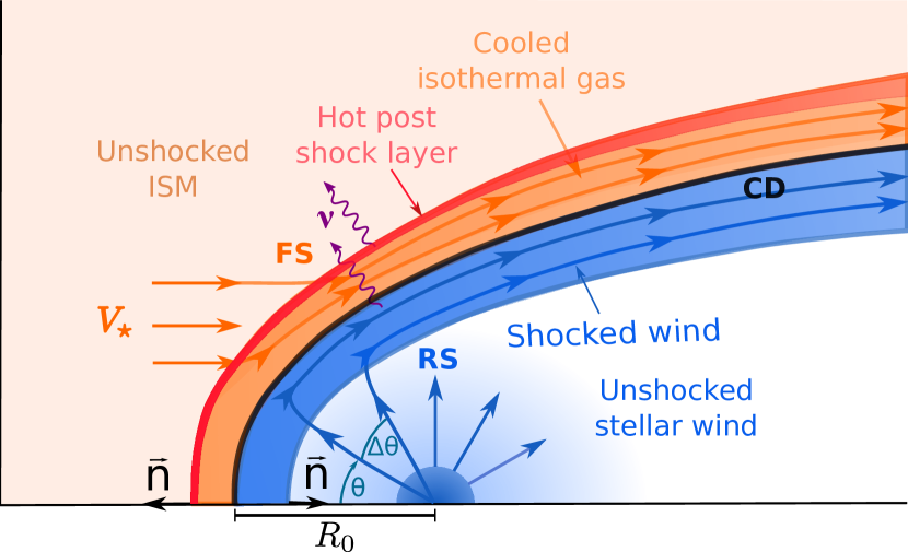
Figure 1: Sketch (not to scale) of a BS of a runaway star. The FS and the RS are separated by the CD, represented by a solid black line. The immediate post-shock external medium, the shocked medium ionised by the star, and the shocked stellar wind are shown in red, orange, and blue, respectively. The solid lines with arrows indicate the shocked gas streamlines, from the injection position up to the tail of the BS. Adapted from Martinez et al. (2022).

The shape of the CD for a star moving through a warm ISM was determined analytically by Christie et al. (2016). We approximated each shock as a thin and axisymmetric structure, co-spatial with the CD, and characterised the BS employing a multi-zone model. Shocked gas convects away from the apex at a fixed angle $\phi$ around the symmetry axis. For a given $\phi$, we discretised each shock in multiple cells, corresponding to different angles $\theta$ measured from the star (with $\theta=0$ at the apex of the BS). Finally, we followed the shocked gas and calculated the thermodynamic quantities cell by cell up to a certain angle, $\theta_{\rm max}$, at which the FS vanishes. Although the RS could still accelerate particles further, the shocked flow will tend to develop instabilities, so we assumed that the RS also stops at $\theta_{\rm max}$. The value of $\theta_{\rm max}$ depends mostly on the velocity of the star: the BS extends up to larger values of $\theta_{\rm max}$ for stars with higher velocities.

The closest position of the CD to the star is the stagnation point. It is located along the CD axis of symmetry, and it is the position where the ISM and the stellar wind pressures cancel each other out. The ISM pressure is a combination of ram and thermal pressure, while in the stellar wind, the thermal pressure is negligible compared to its ram pressure. The position of the stagnation point is then given by

$$R_{0}=\sqrt{\frac{\dot{M}v_{\rm w}}{4\pi\Bigl{(}n_{\rm ISM}k_{\rm B}T_{\rm ISM}+\rho_{\rm ISM}V_{\star}^{2}\Bigr{)}}},$$ (1)

where $\rho_{\rm ISM}=n_{\rm ISM}\,\mu_{\rm ISM}\,m_{p}$ is the density of the ISM, $\mu_{\rm ISM}$ its mean molecular weight, and $m_{p}$ the proton mass.

3.1 Reverse shock

The RS is strong and adiabatic. The shock heats and compresses the stellar wind, also compressing the local magnetic field. Shocked material convects away from the BS apex without cooling, as cooling timescales are much larger than escape timescales. Under such conditions, electrons and protons can be accelerated via diffusive shock acceleration. Electrons emit NT radiation, predominantly synchrotron emission in radio and inverse Compton (IC) emission in X-rays and gamma rays. The IC can be produced by the interaction with the stellar radiation field or the infrared radiation emitted by the heated dust in the FS. On the other hand, proton-proton (p-p) cooling of protons is inefficient, as the shocked wind is very diluted.

3.1.1 Hydrodynamics of the reverse shock

In the star reference frame, the shocked wind is reaccelerated from the BS apex towards distant regions, moving parallel to the CD. In the regions where the shocked wind is subsonic, we assumed that the total pressure from the upstream medium is transformed into thermal pressure in the downstream medium. In the supersonic regime, instead, we considered that only the total momentum flux component that is perpendicular to the BS is converted to thermal pressure. Moreover, we assumed that the shocked fluid behaves as an adiabatic gas with coefficient $\gamma=5/3$. Under this hypothesis, we obtain the density using the polytropic relation, $\rho(\theta)\propto P(\theta)^{1/\gamma}$, and specific enthalpy conservation across the shock front.

The magnetic field in the RS can be generated by adiabatic compression of the star magnetic field and/or generated in situ by the diffusion of cosmic rays (e.g. Pittard et al., 2021). Because of the former, the magnetic field is expected to be parallel to the RS surface (Marcowith et al., 2016). In the subsonic region we calculated it by imposing that the magnetic pressure is a fraction $\eta_{\rm B}$ of the thermal pressure, so

$$B(\theta)=\left[\eta_{\rm B}8\pi P(\theta)\right]^{1/2}.$$ (2)

Here $\eta_{B}<1$: otherwise, the gas becomes incompressible and diffusive shock acceleration cannot take place. Lastly, in the supersonic region we assumed that the magnetic field remains frozen to the plasma. Then we obtained the magnetic field considering conservation of the magnetic flux:

$$B(\theta)=B(\theta_{\mathrm{c}})\,\left(\frac{\rho(\theta)}{\rho(\theta_{\mathrm{c}})}\frac{v(\theta_{\mathrm{c}})}{v(\theta)}\right)^{1/2},$$ (3)

with $\theta_{\rm c}$ the angle at which the plasma becomes supersonic.

3.1.2 Non-thermal particles

We discretised the RS in multiple cells, corresponding to different angles $\theta$. To compute the NT emission we considered several one-dimensional linear emitters. Each of these starts at a different cell and consists of multiple cells located on the path of the emitter along the shock. We assumed that NT particles are injected in the first cell of each emitter, and we summed up the contributions from all the emitters at a certain angle $\phi$, obtaining a one-dimensional set of emitters (a sketch is shown in Fig. 5 in del Palacio et al., 2018). Lastly, we rotated this set around the symmetry axis to get the entire structure of the RS.

We needed to assume an energy distribution of injected NT particles at the i-th cell. For electrons with a power-law energy distribution with spectral index $p$, their synchrotron spectra is also a power law with spectral index $\alpha=\left(p+1\right)/2$ (with $N\left(E\right)\propto E^{p}$ and $S\propto\nu^{\alpha}$). Thus, observations at radio frequencies can be used to derive the injection spectrum. Observations by Benaglia et al. (2021) and Moutzouri et al. (2022) revealed emission with $\alpha\sim-(0.75$–$1)$, consistent with an injection index of $\approx p\approx-(2.5$–$3$). However, assuming a constant injection index of $p=-2.5$ (or $p=-3$) for all electron energies leads to unrealistic energetic requirements in the BS of BD+60°2522 and also to largely over-predicting the flux of the BS of BD+43°3654 at 150 MHz (see Sect. 4.2 for further details). This suggests that the electron energy distribution has a harder spectral index at lower energies. We therefore propose a piecewise injection spectrum:

$$Q\left(E,\theta_{i}\right)=\begin{dcases}Q_{0}\,E^{p_{1}}\exp{\left(-E/E_{\rm max}\right)}&E<E_{\rm break}\sim 2\leavevmode\nobreak\ {\rm GeV}\\ Q_{0}\,E^{p_{2}}\exp{\left(-E/E_{\rm max}\right)}&E\geq E_{\rm break}\sim 2\leavevmode\nobreak\ {\rm GeV}.\end{dcases}$$ (4)

The value of $p_{1}$ is poorly constrained by the available observations, so we simply adopted a hard spectrum below $E_{\rm break}$ with $p_{1}\sim 1$, since softer values lead to overestimating the emission at 150 MHz. Additionally, we set a soft index $p_{2}\sim-3$ above $E_{\rm break}$.

On the other hand, $Q_{0}$ is a normalisation factor and $E_{\rm max}$ a cut-off energy, both dependent on $\theta$. We set the normalisation factor by the condition

$$\int_{2m_{\rm e}c^{2}}^{E_{\rm max}}E\,Q\left(E,\theta_{i}\right)\,{\rm d}E=\Delta L_{\rm NT}\left(\theta_{i}\right)=f_{\rm NT}\,\Delta L_{\perp}\left(\theta_{i}\right),$$ (5)

where $\Delta L_{\rm NT}\left(\theta_{i}\right)$ is the power injected into NT particles at the position $\theta_{i}$. The fraction $f_{\rm NT}$ of the power $\Delta L_{\perp}\left(\theta_{i}\right)$ injected perpendicularly into the RS is a free parameter of the model, while $\Delta L_{\perp}(\theta_{i})$ depends on the RS region:

$$\Delta L_{\perp}(\theta_{i})=\begin{dcases}0.5\,\rho_{\rm w}(\theta_{i})\,v_{\rm w}^{3}\,\Delta A_{\perp}(\theta_{i})\quad{\rm(subsonic\;region)}\\ 0.5\,\rho_{\rm w}(\theta_{i})\,v_{\rm w}^{2}\,v_{{\rm w}\perp}(\theta_{i})\,\Delta A_{\perp}(\theta_{i})\quad{\rm(supersonic\;region)},\end{dcases}$$ (6)

with $\Delta A_{\perp}(\theta_{i})$ the area of the i-th cell perpendicular to ${\bf v_{\rm w}}$. In turn, a fraction $\Delta L_{\rm NT,e}(\theta_{i})=f_{{\rm NT,}e}\,\Delta L_{\perp}(\theta_{i})$ is injected into electrons, while the remaining fraction, $f_{{\rm NT,}p}=f_{\rm NT}-f_{{\rm NT,}e}$, is injected into protons. Finally, the cut-off energy is obtained by equating the acceleration and energy timescales.

We notice that the magnetic field plays an important role in the acceleration of particles. Although we supposed that the field lines are mostly parallel to the BS surface, we addressed the acceleration process phenomenologically, and different geometries would lead to similar results. For instance, shock drift acceleration could also take place, but the shape of the energy particle distribution would be unaltered if particles can complete enough acceleration cycles (Matthews et al., 2020).

We approximated the steady-state particle distribution at the injection cell by:

$$N_{0}\left(E,\theta_{i}\right)\approx Q\left(E,\theta_{i}\right)\times{\rm min}\left(t_{\rm cell},t_{\rm cool}\right),$$ (7)

with $t_{\rm cell}$ the cell convection time and $t_{\rm cool}$ the cooling timescale of NT particles. Lastly, we considered convection by the shocked gas and calculated the particle energy distribution cell by cell assuming conservation of the flux of particles in the space of energy and positions. As an example, in Fig. 2 we show the resulting electron energy distribution for the BS of BD+43°3654. For further details of the RS treatment, we refer the reader to Martinez et al. (2022).

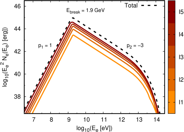
Figure 2: Electron energy distribution for the RS of the BS of BD+43°3654. We discretise the distribution in five segments of length $\theta_{\rm max}/5$ along the BS (colour scale, with I1 the one starting at the apex of the BS). The dashed black line shows the total distribution. The adopted injection function is given by Eq. 4.

3.2 Forward shock

The FS is a radiative shock that compresses and heats the oncoming ISM material. This creates a thin hot post-shock layer where injected power is re-emitted via thermal bremsstrahlung and line emission (Gull & Sofia, 1979). Moreover, early-type runaway stars present wind-driven BSs in which the star photo-ionises the entire BS structure (Henney & Arthur, 2019). Consequently, there are two layers in the FS: a hot immediate post-shock layer that cools locally, and an isothermal layer (IL) with a temperature $T\sim 8\,000$ K that is kept warm and ionised by the star (Mackey, 2022), as shown in Fig. 1. Henceforth we will refer to the former as the hot layer (HL) and the latter as the isothermal layer. We note that, although particles can be accelerated in low-Mach-number shocks, a stellar velocity of hundreds of km s^-1 is required for this to be efficient (Martinez et al., 2022). Thus, we considered only thermal radiation from the FS.

3.2.1 Hydrodynamics of the forward shock

We employed Rankine-Hugoniot jump conditions to determine the thermodynamic quantities in the HL. We calculated the density in terms of the ISM density and the compression factor:

$$\rho_{\rm HL}(\theta)=\zeta(\theta)\,\rho_{\rm ISM},$$ (8)

and the pressure in terms of the Mach number and the ISM thermal pressure:

$$P_{\rm HL}(\theta)=\left(\frac{2\gamma M(\theta)^{2}-\gamma+1}{\gamma-1}\right)\,P_{\rm th,ISM}.$$ (9)

The ISM thermal pressure depends on the ISM temperature and numerical density as $P_{\rm th,ISM}=n_{\rm ISM}k_{\rm B}T_{\rm ISM}$. As runaway stars are ejected from their birth clusters at high velocities and are usually isolated, it is unlikely that other sources could affect the properties of their surrounding ISM. Thus, we focused on the case of wind-driven BSs with Strömgren spheres that are much larger than the BS itself. Under these considerations, we expect an ionised ISM with temperature $T_{\rm ISM}\sim 8\,000\leavevmode\nobreak\$K (Weaver et al., 1977).

The temperature of the HL is also determined in terms of the Mach number and the ISM temperature:

$$T_{\rm HL}(\theta)=\frac{\left[\left(\gamma-1\right)M(\theta)^{2}+2\right]\left[2\gamma M(\theta)^{2}-\left(\gamma-1\right)\right]}{\left(\gamma+1\right)^{2}M(\theta)^{2}}\,T_{\rm ISM}.$$ (10)

Using this expression we fixed $\theta_{\rm max}$ as the angle at which $\rho(\theta)\approx\rho_{\rm ISM}$, where the FS vanishes.

Knowing the temperature of the HL enables the calculation of the density of the IL. Given that the pressure at the IL is $P_{\rm IL}(\theta)=P_{\rm HL}(\theta)$ because of pressure equilibrium, the density increases with respect to $\rho_{\rm HL}(\theta)$ by a factor $T_{\rm HL}(\theta)/T_{\rm IL}$:

$$\rho_{\rm IL}\left(\theta\right)=\frac{P_{\rm HL}(\theta)}{k_{\rm B}T_{\rm IL}}\,\mu\,m_{p}=\frac{T_{\rm HL}(\theta)}{T_{\rm IL}}\,\rho_{\rm HL}(\theta),$$ (11)

where $\mu\approx 0.6$ is the mean molecular weight (assuming solar abundances).

Lastly, considering mass conservation across the shock, the width of the IL region is:

$$H_{\rm IL}(\theta)=\eta_{\rm H}\left[\frac{\int_{0}^{\theta}\rho_{\rm ISM}(\theta^{\prime})\,V_{\star}\,A_{\perp}(\theta^{\prime})\,{\rm d}\theta^{\prime}}{2\pi\,R(\theta)\,\sin{(\theta)}\,\rho_{\rm IL}(\theta)\,v_{\parallel}(\theta)}-\left(\frac{\rho_{\rm HL}(\theta)}{\rho_{\rm IL}(\theta)}\right)H_{\rm HL}(\theta)\right],$$ (12)

where $v_{\parallel}(\theta)$ is the convection velocity of the shocked fluid, and $H_{\rm HL}\left(\theta\right)=\left(V_{\star\perp}/\zeta\right)t_{\rm cool,HL}$ the width of the HL. Finally, $\eta_{\rm H}\leq 1$ is a free parameter that accounts for additional processes not included in the model that can reduce the IL thickness, such as thermal conduction and instabilities (e.g. Comeron & Kaper, 1998).

3.2.2 Thermal emission

Thermal radiation from the HL and the IL is optically thin. We calculated their free–free spectral luminosity as (e.g. Rybicki & Lightman, 1986):

$$L_{\rm ff}(\theta,\epsilon_{\rm ph})=6.38\times 10^{-38}\frac{L_{0}\,Z^{2}\,n_{\rm e}\,n_{\rm i}\,g_{\rm ff}\,\epsilon_{\rm ph}}{\sqrt{T}}\,\exp{\left(-\frac{\epsilon_{\rm ph}}{k_{\rm B}T}\right)}\;{\rm erg\,s^{-1}},$$ (13)

where all quantities are in cgs units. In this formula, $Z$ is the mean atomic number (assumed to be $Z=0.79$ for solar abundances and typical conditions of an HII region), $g_{\rm ff}$ the mean Gaunt factor, $\epsilon_{\rm ph}$ the energy of the photons, $n_{\rm i}\approx n_{\rm e}\approx n/2$ the ion and electron number densities, respectively, and $L_{0}$ a normalisation factor.

The total free–free luminosity from the HL depends mostly on the velocity of the star and the density of the ISM, and it is normalised at each cell by the condition:

$$L_{\rm ff,HL}(\theta_{i})=\frac{\Lambda_{\rm ff}(T)}{\Lambda_{\rm tot}(T)}\left(1-\frac{T_{\rm IL}}{T_{\rm HL}(\theta_{i})}\right)\,L_{\perp}(\theta_{i}),$$ (14)

with $L_{\perp}(\theta_{i})=0.5\,\rho_{\rm ISM}\,V_{\star}^{2}\,V_{\star\perp}(\theta_{i})\,A_{\perp}(\theta_{i})$, and $\Lambda_{\rm ff}$ and $\Lambda_{\rm tot}$ are the free–free and total cooling coefficients, respectively (Myasnikov et al., 1998). On the other hand, the normalisation of the emission from the IL layer is determined by the volume of the cell:

$$L_{0}=\Delta V(\theta)=2\,\pi\,R(\theta)\sin{(\theta)}\,H_{\rm IL}(\theta)\,\Delta l(\theta),$$ (15)

where $\Delta l(\theta)$ is the length of the corresponding cell.

3.3 Beyond the bow shock region

OB stars have strong UV radiation fields that ionise their surrounding media. If the star is supersonic, the size of the ionised region can be approximated as the size of the Strömgren sphere (Tenorio Tagle et al., 1979):

$$R_{\rm Str}=0.68\,{\rm pc}\,\left(\frac{Q_{\rm ion}}{10^{49}\,{\rm s^{-1}}}\right)^{1/3}\,\left(\frac{n}{10^{3}\,{\rm cm^{-3}}}\right)^{-2/3}\,\left(\frac{T}{10^{4}\,{\rm K}}\right)^{0.28},$$ (16)

with $Q_{\rm ion}$ the ionising photon injection rate of the star and $n$ the numerical density of the neutral ISM (Lacki, 2013).

In turn, a fraction of NT particles escape from the BS region without radiating significantly. These particles may diffuse and convect inside the ionised ISM, interacting with the local radiation and mass fields and producing multi-wavelength radiation. We focused on gamma rays and used a simplified one-zone model to estimate their luminosity, as this is the most conspicuous component of this emission.

Let $L_{\rm NT}$ and $L_{\rm BS,e(p)}$ be the luminosity injected into and radiated by electrons (protons) in the BS. The cosmic-ray luminosity injected in the ionised ISM is $L_{\rm HII,e(p)}$ = $L_{\rm NT,e(p)}-L_{\rm BS,e(p)}$. In turn, the fraction of this luminosity radiated by a certain radiation process can be estimated as

$$L_{\rm rad,e(p)}\sim\frac{t_{\rm esc,e(p)}}{t_{\rm rad,e(p)}}L_{\rm HII,e(p)},$$ (17)

where $t_{\rm esc}$ and $t_{\rm rad}$ are the escape timescale and radiation process cooling timescale, respectively (formula valid for $t_{\rm esc}<t_{\rm rad}$). We calculated the former in terms of the convection and diffusion timescales, $t_{\rm esc}^{-1}=\left(t_{\rm conv}^{-1}+t_{\rm dif}^{-1}\right)^{-1}$. In particular, $t_{\rm conv}=R_{\rm HII}/V_{\star}$, and we adopted the diffusion coefficient proposed by Gabici et al. (2007), which is suitable for these structures:

$$t_{\rm diff}=\frac{R_{\rm HII}^{2}}{6D_{\rm diff}};\quad D_{\rm diff}=3\times 10^{27}\chi\left(\frac{E/{\rm GeV}}{B/\left(3{\rm\mu G}\right)}\right)^{0.5}\;{\rm cm^{2}\,s^{-1}},$$ (18)

with $\chi<1$. We fixed $\chi=0.1$ and $B=10$ $\mu$G (Gabici et al., 2007), which yields $D_{\rm diff}\approx 2\times 10^{26}$ cm² s^-1 at 1 GeV, adopted as the energy reference for both protons and electrons.

Relativistic particles can interact with the ambient nuclei from the ionised region leading to the emission of gamma-ray photons. For relativistic protons, these interactions are p-p collisions in which the resultant neutral pions decay into gamma rays, while relativistic electrons interact with the nuclei electrostatic field and emit NT bremsstrahlung. If $\mu$ is the mean molecular weight ($\mu\approx 0.6$ for a fully ionised gas with solar abundances), and $n_{\rm ISM}$ the number density inside the sphere, the ambient proton density is $n_{p}=\mu\,n_{\rm ISM}$. Then, the p-p and NT-bremsstrahlung timescales are (Atoyan et al., 1995; Aharonian & Atoyan, 1996)

$$t_{\rm p-p}\approx t_{\rm br}\approx 10^{15}\,\left(\frac{n_{p}}{\mathrm{cm}^{-3}}\right)^{-1}\leavevmode\nobreak\ \mathrm{s}.$$ (19)

Approximately 15% of the energy available in each p-p collision goes to gamma rays (Kelner et al., 2006). Moreover, if the proton energy distribution also peaks at $E_{p}\sim 1$ GeV, as is the case here, the p-p SED peaks at $\epsilon\sim 100$ MeV. Taking into account the fact that ionisation losses are not dominant at energies $E\gtrsim 1$ GeV (Atoyan et al., 1995), we approximated the gamma-ray luminosity as

$$L_{\rm\epsilon,p-p}(\gtrsim 100\leavevmode\nobreak\ {\rm MeV})\sim 0.1\;\left(\frac{t_{\rm esc}}{t_{\rm p-p}}\right)\;L_{\rm HII,p}.$$ (20)

On the other hand, the NT-Bremsstrahlung SED peaks at $\epsilon\sim 1$ GeV. In this case, most of the radiation is emitted around that energy, so that we can approximate

$$L_{\rm\epsilon,br}(\gtrsim 1\leavevmode\nobreak\ {\rm GeV})\sim\left(\frac{t_{\rm esc}}{t_{\rm br}}\right)\;L_{\rm HII,e}.$$ (21)

In addition, p-p collisions also lead to electron–positron pair production. These secondary electrons could also contribute to the NT-Bremsstrahlung SED. However, their luminosity would be approximately half that in p-p gamma rays, and thus the p-p gamma-ray luminosities estimated above are already correct within an order of magnitude.

4 Results and discussion

4.1 Thermodynamics

As an example, in Fig. 3 we show the most relevant thermodynamic quantities from the RS and the FS of the BS of BD+43°3654 as a function of the angle $\theta$, up to the angle $\theta_{\rm max}$. In particular, we set $\theta_{\rm max}=120\degree$ for BD+43°3654 and BD+60°2522, $\theta_{\rm max}=135\degree$ for Vela-X1, $\theta_{\rm max}=80\degree$ for G1 and $\theta_{\rm max}=90\degree$ for G3, using the criteria mentioned in Sect. 3.2.1.

Given that the FS of the BS of BD+43°3654 is not hypersonic but $M(\theta)\gtrsim 1$, the resulting density in the HL (Eq. 8) is $\rho_{\rm HL}(\theta)\sim 3\,\rho_{\rm ISM}$, below typical values for strong shock conditions. The conversion of kinetic energy into thermal energy is more efficient for small values of $\theta$, and the shocked ISM reaches temperatures of $T_{\rm HL}\sim 70\,000\leavevmode\nobreak\$K near the apex. Because of cooling, the shocked ISM material is compressed in the IL due to the corresponding temperature decrease, and the density reaches values above $10\,\rho_{\rm ISM}$ up to an angle $\theta\sim 85\degree$.

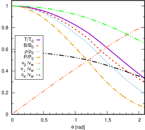
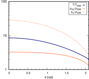
Figure 3: Thermodynamical quantities along the BS of BD+43°3654. Left panel: Thermodynamic variables in the RS as a function of $\theta$. The temperature, magnetic field, density, and pressure are normalised to their values at the apex ($\theta=0$), while the tangential, perpendicular, and sound velocities are normalised to the stellar wind velocity. Right panel: Density of the IL (dotted coral line) and HL (solid coral line) and temperature of the HL (blue solid line), all as a function of the angle $\theta$; the variables are normalised to the un-shocked ISM values.

4.2 Radio emission

The synchrotron radiation from the RS depends on the magnetic field, which is determined by the pressure in the subsonic region, and by the velocity and density of the fluid after the sonic point. Figure 3 shows that the pressure in the RS decays with $\theta$ as the shock becomes more oblique. As a result, the magnetic field also decays gradually, leading to stronger synchrotron emission near the apex. This is consistent with the morphology and brightness distribution seen in the resolved images of BSs (Benaglia et al., 2010; Moutzouri et al., 2022).

Regarding the FS, the free–free emission from both the HL and the IL depends on the density and temperature, as shown in Eqs. (13 – 14). In particular, the high temperature of the HL makes its free–free emission negligible at radio frequencies, as $\Lambda_{\rm ff}(T)/\Lambda_{\rm tot}(T)\ll 1$. On the other hand, the IL emission could be important at radio, although the layer (and therefore its emission) could be reduced significantly because of instabilities (see Sects. 4.2.1 and 4.2.2 for further details).

4.2.1 BD+43°3654

In Fig. 4 we show the radio SED of the BS of BD+43°3654 together with the data from Benaglia et al. (2010), Benaglia et al. (2021), and Moutzouri et al. (2022) and our estimate from Appendix A. In particular, we considered the VLA observations from Benaglia et al. (2010) as lower limits, as they were not sensitive enough to reach the fainter emission from the more extended regions of the BS and thus underestimated the total integrated fluxes. We also show two SEDs reported by Benaglia et al. (2021). One of them integrated the flux densities within contours above 1.5 mJy beam^-1, while the other considered contours above 2.3 mJy beam^-1; hereafter we refer to these datasets as B2021–A and B2021–B, respectively. The contours selected in B2021–A may include regions that do not correspond to the BS, as inferred from infrared emission maps from WISE (see Fig. 1 in Moutzouri et al., 2022). We thus considered that the reported fluxes in B2021–A could be overestimated, and those of B2021–B are more representative of the true spectrum of the BS.

We find that the predicted free–free emission for $\eta_{\rm H}=1$ is too high: it overestimates the radio fluxes by a factor of $\sim 2$ and leads to a thermal-dominated spectrum, in discordance with the observed spectral indices. We thus imposed $\eta_{\rm H}<0.3$ to be consistent with the available data, meaning that the IL is significantly reduced. Kelvin Helmholtz instabilities can justify this drastic reduction in the IL due to the difference between the RS and the FS shocked flow velocities (Comeron & Kaper, 1998). However, characterising the phenomena that produce these effects is beyond the scope of this paper.

Just as a reference, we considered that $\sim 15$% of the injected power in the RS goes to cosmic rays (that is, $f_{\mathrm{NT}}\sim 0.15$) and, to explain observations, that 10% of that power must go to electrons (leading to $f_{\mathrm{NT,e}}\sim 0.015$). In addition, we fixed the magnetic field setting $\eta_{\rm B}\sim 0.2$; the adopted parameters are summarised in Table 2. The value of $\eta_{\rm B}\sim 0.2$ would be consistent with the adiabatic compression of magnetic field lines from the stellar wind for a surface stellar magnetic field of $B_{\star}\sim 300$ G (del Palacio et al., 2018). We note that slightly different choices of parameters can also lead to a similar spectrum, but the overall conclusions would not be affected and thus, for simplicity, we took the aforementioned values as representative.

The luminosity injected into cosmic rays is at least $L_{\rm NT}\sim 10^{35}\leavevmode\nobreak\$erg s^-1, in the form of NT electrons, which is $\sim 1.5$% and $\sim 0.8$% of the shocked and the total wind luminosity, $L_{\rm w}=0.5\,\dot{M}\,v_{\rm w}^{2}$, respectively. However, the energy in hadronic cosmic rays may be potentially much higher, so $L_{\rm NT}\gtrsim 10^{36}\leavevmode\nobreak\$erg s^-1 are plausible. The magnetic field results in $B\sim 30\leavevmode\nobreak\ \mu$G near the apex, and the ratio between the magnetic and NT electron energy densities is $U_{\rm B}/U_{\rm NT,e}\sim 4$, above (but not very far from) equipartition of $B$ with NT electrons. Regarding the maximum energies, both electrons and protons reach energies of $E_{\rm max}\lesssim 100$ TeV near the apex assuming Bohm diffusion. In addition, our model predicts radio fluxes consistent with B2021–B, whereas reaching the flux densities from B2021–A would require even more extreme parameters, which also supports the choice of B2021–B. Finally, we also verified that the predicted NT emission in X-rays (mostly synchrotron) between 0.4 and 4 keV is $L_{\rm X}=2\,\times\,10^{30}\leavevmode\nobreak\$erg s^-1, consistent with the upper limit of $L_{\rm X}<7.6\,\times\,10^{30}\leavevmode\nobreak\$erg s^-1 (Toalá et al., 2016).

Brookes (2016), Benaglia et al. (2021), and Moutzouri et al. (2022) reported emission maps of BD+43°3654 at 325 MHz, 3 GHz, and 4–12 GHz, respectively. In Fig. 5 we show our synthetic maps at those same frequencies. Our model successfully reproduces the spatial morphology observed on a qualitative level: the BS is brighter at the apex, where the shock is stronger and the magnetic field is $B\sim 30\leavevmode\nobreak\ {\rm\mu G}$, and the angular extension also matches the observed one. On a more quantitative level, the contour levels of the synthetic map at 3 GHz follow the same emission contours as the observed map, while the maps at 325 MHz and 4–12 GHz slightly overestimate the surface brightness by factors of $\sim 1.5$ and $\sim 2$, respectively. Nevertheless, the uncertainty on $V_{\star,r}$ can also affect these results, as larger values of $V_{\star,{\rm r}}$ lead to a more extended BS in the plane of the sky, diluting the surface brightness.

Finally, we produced synthetic emission maps at 150 MHz using two different injection prescriptions. In Fig. 6 (top) we use an injection function with a single spectral index $p=-2.55$, while in Fig. 6 (bottom) we use the piecewise function from Eq. (4). The single index prescription overestimates the fluxes at 150 MHz by a factor of $\sim 7$ (see Appendix A). On the other hand, the piecewise injection is consistent with the non-detection of the BS above (3-$\sigma$) noise levels of $\gtrsim 20$  mJy beam^-1. In addition, using the single index prescription requires fixing $\eta_{\rm B}\approx 0.4$ and that $\sim 40\%$ of $\Delta L_{\perp}$ goes to electrons to fit the spectrum between 1 and 12 GHz. Given that these assumptions are very extreme, and that the single index prescription largely overestimates the radiation at 150 MHz, we conclude that a piecewise injection function is needed.

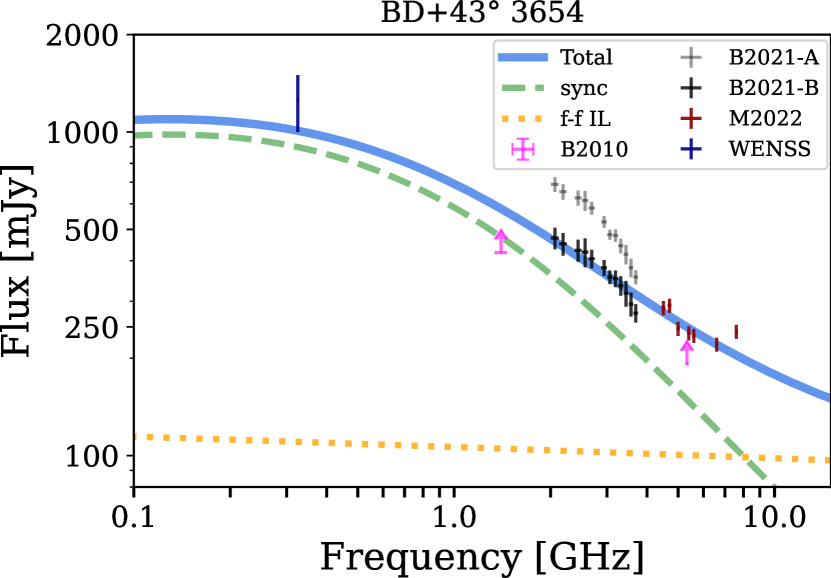
Figure 4: SED of the BS of BD+43°3654 between 100 MHz and 15 GHz. The dashed green, dotted orange, and solid light blue lines are the synchrotron, free–free (IL) and total emission curves calculated with our model. The magenta arrows are the lower limits of Benaglia et al. (2010). The grey data points show the SED reported by Benaglia et al. (2021) when selecting contours ¿ 1.5  mJy beam^-1, and the black data points show the SED from contours ¿ 2.3  mJy beam^-1. The dark red data points show the SED reported by Moutzouri et al. (2022). The dark blue bar is the total flux obtained from the WENSS emission map at 325 MHz (Appendix A).

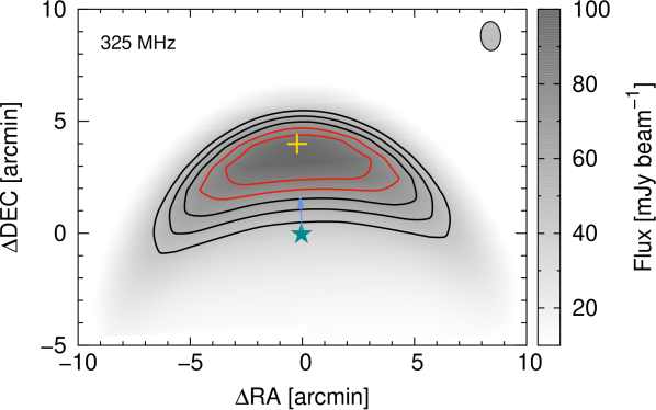
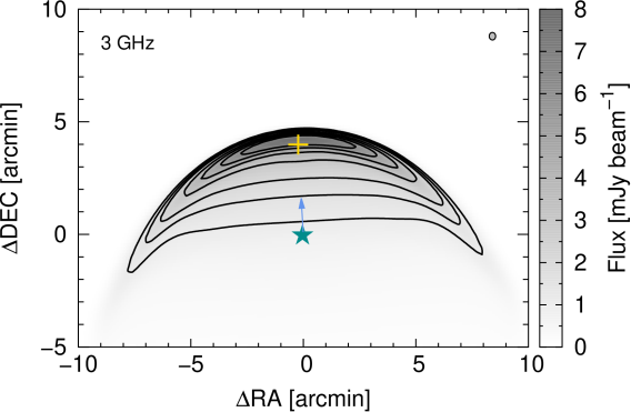
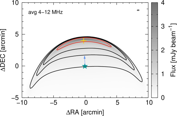
Figure 5: Simulated emission maps of the BS of BD+43°3654. Black contours match the observed ones, while red contours are above them. Top panel: Map at 325 MHz with a beam size of $54"\times 77"$. Black contour levels are 44, 54, and 64  mJy beam^-1; red contour levels are 74 and 84  mJy beam^-1. Middle panel: Map at 3 GHz with a beam size of $20.2"\times 12.5"$. Contour levels are 1, 1.5, 2, 3, 4, 5, and 6  mJy beam^-1. Bottom panel: Average map at 4–12 GHz with a beam size of $20"\times 10"$. Black contour levels are 0.3, 0.6, and 0.9  mJy beam^-1; the red contour level is 1.8  mJy beam^-1.

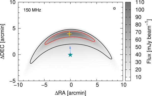
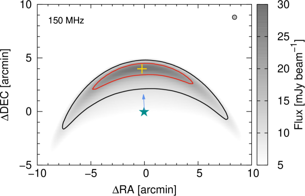
Figure 6: Simulated emission maps of the BS of BD+43°3654 at 150 MHz using the single index injection (top panel) and the piecewise injection (bottom panel). The beam size is $25"\times 25"$. The black contour is 10  mJy beam^-1 (similar to the rms of the map from the TGSS survey; see Fig. 10), while the red contour levels are 20, 40, 80, and 120  mJy beam^-1.

4.2.2 BD+60°2522

The spectral index derived by Moutzouri et al. (2022) at 4–12 GHz also implies a steep energy distribution of relativistic electrons with energies from $\sim 1$ GeV to at least $\sim$10 GeV. To recover this steep radio spectrum requires a reduction in the IL ($\eta_{\rm H}<0.15$). Moreover, the available luminosity in the RS is insufficient to explain the observed synchrotron SED with the single index prescription, so the electron distribution should be much harder below $\sim 1$ GeV. We thus adopted the injection spectrum from Eq. (4), assumed that $\sim 5$% of the kinetic energy is converted into electrons, and set the reference value $\eta_{B}\approx 0.2$, which yields a magnetic field of $50\leavevmode\nobreak\ \mu$G near the apex.

In Fig. 7 we show two synthetic emission maps of the BS of BD+60°2522. In Fig. 7 (top) we show the average emission between 4 and 12 GHz, while in Fig. 7 (bottom) we predict the observed emission at 110 MHz. We note that our modelled map is in good accordance with the flux density of $\sim 6$  mJy beam^-1 near the apex of the BS seen in Fig. 1 of Moutzouri et al. (2022). However, we highlight that the total luminosity reported by Moutzouri et al. (2022) is most likely to be highly overestimated due to the presence of dense, ionised clumps to the west of BD+60°2522 (Moore et al., 2002). These clumps emit bright thermal emission that dominates the single-dish observations between 4 and 12 GHz.

We also predict integrated fluxes of $\sim 110$ mJy at 150 MHz and $\sim 120$ mJy at 325 MHz from the BS of BD+60°2522. However, these values depend strongly on the assumed electron energy distribution below $\sim 1$ GeV, which can only be inferred directly by measuring their synchrotron emission at $\nu\sim 100$ MHz. Hence, low-frequency, high-angular-resolution observations would allow us to better constrain the injection spectrum, and therefore the particle acceleration processes in the BS.

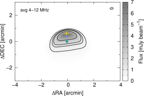
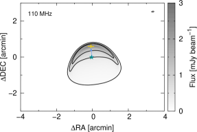
Figure 7: Simulated emission maps of the BS of BD+60°2522. Top panel: Average map between 4 and 12 GHz. The contour levels are 0.5, 1, 1.5, and 3 mJy beam^-1. Bottom panel: Map at 110 MHz. The beam size is $4"\times 4"$, and the contour levels are 0.1, 0.5, and 1  mJy beam^-1.

4.3 G1, G3, and Vela X-1

In Fig. 8 we show the SEDs for the sample of BSs reported by van den Eijnden et al. (2022b) and van den Eijnden et al. (2022a). For the case of G1, the flux density observed at 887.5 MHz cannot be explained solely as thermal emission, as even considering $\eta_{\mathrm{H}}=1$ yields a flux density of $\approx 5$ mJy and the observed flux is $\approx 9$ mJy. Moreover, the better studied BSs seem to suggest values of $\eta_{\mathrm{H}}<0.3$. On the other hand, a purely NT scenario requires a high –but not unrealistic– conversion of kinetic energy into NT energy. As a reference case, we can explain the observed flux density with a significant synchrotron contribution adopting $\eta_{\mathrm{H}}=0.1$, $\eta_{\rm B}=0.2$ and $f_{{\rm NT,e}}=0.03$. However, it is not currently possible to determine which component is dominant in this system, as hybrid scenarios are also plausible.

For the case of G3, assuming $\eta_{H}=1$ overestimates the fluxes by a factor of $\sim 2$. Thus, the emission can be of thermal origin if the IL width parameter is $\eta_{H}\sim 0.45$. Alternatively, we can explain the spectrum with reasonable NT parameters by setting $\eta_{\rm B}=0.2$ as a reference value and assuming that $f_{{\rm NT,e}}=0.01$. Although G1 and G3 have similar parameters, the reported mass loss rate of the latter is almost twice as large, favouring a NT-dominated scenario (as the synchrotron luminosity scales roughly as $\propto\dot{M}_{\mathrm{w}}^{1.5}$; del Palacio et al., 2018). The similarities between the parameters assumed for BD+43°3654 and BD+60°2522, and the NT scenario of G1 and G3, could suggest that indeed in G1 and G3 the radio spectrum can be dominated by synchrotron emission and that the IL is significantly evaporated. We note that this interpretation is in tension with that of van den Eijnden et al. (2022b), who favoured a thermally dominated scenario for the systems G1 and G3. Nonetheless, our more detailed model considers an injection function of NT particles that relaxes the energy budget in a NT scenario and reconciles such a scenario with the observations better. Unfortunately, the large uncertainties in the system parameters together with the lack of a good spectral coverage of G1 and G3 prevent us from firmly concluding on the nature of their radio emission.

Finally, for Vela X-1 we obtain that a NT-dominated scenario can explain the observed radio flux density for reasonable parameters, but the BS cannot be solely thermal. Considering $\eta_{\rm H}=1$ yields a free-free flux density of $\approx 4$ mJy at 887.5 MHz, slightly below the $\approx 6$ mJy observed. In the NT scenario, we assumed that $\sim 1\%$ of the available kinetic energy in the RS shock goes to electrons, while we set $\eta_{\rm B}=0.2$. This leads to a magnetic-to-NT electron energy density ratio of $U_{\rm B}/U_{\rm NT,e}\sim 5$, and an upper limit for the IL width of $\eta_{\rm H}<0.3$. Moreover, a NT-dominated scenario is supported by analysis of the observed H_α emission from the BS. We can explain the peak surface brightness of H_α reported by Gvaramadze et al. (2018) by setting $\eta_{\rm H}=0.1$ (see Appendix B). This result strongly encourages the interpretation of a synchrotron-dominated spectrum in Vela X-1 and the significant evaporation of the IL. We note that van den Eijnden et al. (2022a) favoured a thermal scenario for Vela X-1 based on matching the peak brightness in H_α using a one-zone model. Nonetheless, one-zone models are not as adequate as multi-zone models to interpret information from emission maps.

Table 2: Main results regarding the radio emission from the modelled stellar BSs. Column 3 shows the power injected in the RS by the stellar wind typically, $L_{\rm w\perp}\approx 0.5-0.7L_{\rm w}$). Columns 4–6 are model parameters: the fraction of the injected power that goes into electrons, the electrons-to-magnetic energy density ratio, and the IL width parameter; we fix $\eta_{\rm B}=0.2$ for all systems. Column 7 summarises our conclusions about the origin of the emission of each source.

System	Radiation type	$L_{\rm w\perp}$ [erg s-1]	$f_{\rm NT,e}$	$U_{\rm B}/U_{\rm NT,e}$	$\eta_{\rm H}$	Comments
BD+43°3654	NT	$\approx 7\times 10^{36}$	0.013	$\sim 4$	¡ 0.3	The observed spectral index at $\nu>1$ GHz implies a NT spectrum.
BD+60°2522	NT	$\approx 1\times 10^{36}$	0.04	$\sim 1.5$	¡ 0.15	The observed spectral index at $\nu>1$ GHz implies a NT spectrum.
G1	Hybrid/NT	$\approx 1\times 10^{35}$	0.03	$\sim 2$	0.1	The observed flux density at 887.5 MHz cannot be solely thermal and is most likely dominated by NT emission.
G3	NT	$\approx 2\times 10^{35}$	0.01	$\sim 6$	¡ 0.1	The nature of the emission is inconclusive due to uncertainties in $\dot{M}_{\mathrm{w}}$ and the lack of broadband spectral coverage.
	Thermal		¡ 0.002	¿ 30	0.45
Vela X-1	NT	$\approx 1\times 10^{35}$	0.013	$\sim 5$	¡ 0.3	A reduction in the IL is needed to reproduce the Hα surface brightness, and the observed flux density at 887.5 MHz cannot be solely thermal. A NT-dominated spectrum is thus favoured.
	Thermal		¡ 0.003	¿ 25	1

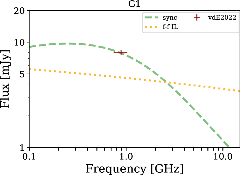
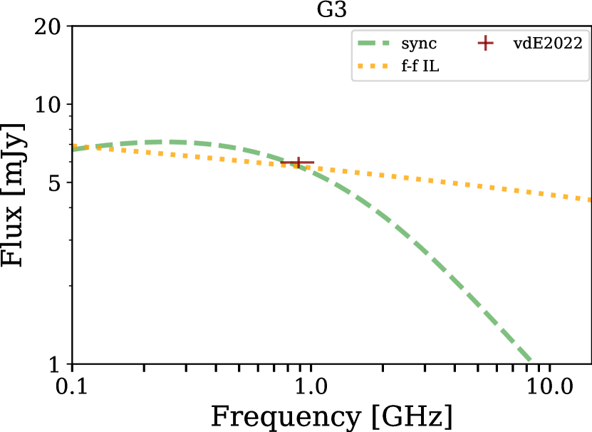
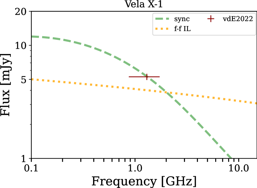
Figure 8: Modelled SEDs between 100 MHz and 15 GHz for G1 (top), G3 (middle), and Vela X-1 (bottom panel). In all cases, we consider two different scenarios: a NT one with a synchrotron spectrum (dashed green line) and a thermal one with free-free emission (dotted orange line). The red cross is the flux reported by van den Eijnden et al. (2022b) for G1 and G3, and by van den Eijnden et al. (2022a) for Vela X-1.

4.4 Gamma-ray emission

We applied the prescription described in Sect. 3.3 to the confirmed NT BSs: BD+43°3654 and BD+60°2522. In both systems, the behaviour of NT particles along the BS is dominated by advection. In consequence, $L_{\rm BS}\ll L_{\rm NT}$ and particles escape from the BS without cooling significantly, and thus $L_{\rm HII}\approx L_{\rm NT}$.

According to Eq. (16), the HII region around BD+43°3654 has a radius of $\sim 20$ pc. For the value of $D_{\rm diff}\approx 2\times 10^{26}$ cm² s^-1 obtained above (note that Bohm diffusion yields $D_{\rm diff}\sim 6\times 10^{22}\leavevmode\nobreak\$cm² s^-1), diffusion dominates the escape, with a timescale of $t_{\rm diff}\approx 3\times 10^{12}$ s. On the other hand, p-p and NT-bremsstrahlung timescales are much greater: $t_{\rm p-p}\sim t_{\rm br}\sim 3\times 10^{14}$. Then, particles may also diffuse from the HII sphere without radiating a significant fraction of their energy as high-energy photons. We estimate luminosities $L_{\rm\epsilon,p-p}(\gtrsim 100\,{\rm MeV})\sim L_{\rm\epsilon,br}(\gtrsim 1\,{\rm GeV})\sim 10^{33}$ erg s^-1, if we assume $f_{\rm NT,e}=0.1\,f_{\rm NT,p}\approx f_{\rm NT}$. According to our model, the emission from the HII region could dominate the spectrum at gamma rays, as the IC luminosity from the BS at 1 GeV would be $L_{\rm\epsilon,IC}(\gtrsim 1\,{\rm GeV})\sim 10^{31}$ erg s^-1. Additionally, the IC emission from the HII region with the cosmic microwave background and the star photon fields are negligible at gamma rays, as the SED from the former peaks at lower energies, while the latter is $L_{\rm IC}\propto U_{\star}\propto R^{-2}$. Lastly, we notice that the derived 0.1–1 GeV luminosities, reachable already only with primary electrons, are close to the upper limits found by Schulz et al. (2014) (also $\sim 10^{33}$ erg s^-1), so the values taken above seem to suggest that BD+43°3654 may be detectable in the near future. Alternatively, a lack of detection would provide constraints on the adopted parameters, in particular on the diffusion coefficient, which is the most uncertain of all.

Our model estimates a Strömgren sphere of $\sim 4$ pc for BD+60°2522. This smaller value is because of the much denser ISM and the later spectral type of the star compared with BD+43°3654. Again, diffusion dominates the timescales, being $t_{\rm diff}\approx 10^{11}$ s, while $t_{\rm p-p}\sim t_{\rm br}\sim 8\times 10^{13}$ s. Adopting $f_{\rm NT,e}=0.2\,f_{\rm NT,p}\approx f_{\rm NT}$ for this source, we estimate that the luminosity injected into NT particles in the BS is $L_{\rm NT}\sim 2\times 10^{35}$ erg s^-1. Taking into account this and the cooling timescales, we estimate gamma-ray luminosities emitted in the HII region around BD+60°2522 of $L_{\rm\epsilon,p-p}(\gtrsim 100\,{\rm MeV})\sim 10^{31}$, and $L_{\rm\epsilon,br}(\gtrsim 1\,{\rm GeV})\sim 10^{32}$ erg s^-1 from primary electrons.

Finally, regarding G1, G3 and Vela X-1, the energetics of their BSs make the systems undetectable at gamma rays with current instruments. In conclusion, our model predicts that the HII region around BD+43°3654 could be detectable with the Fermi-Large Area Telescope (LAT). It is worth adding that the steepness of the electron energy distribution for BD+43°3654 makes this source difficult to detect above 100 GeV (see H. E. S. S. Collaboration et al., 2018, for upper limits of other BSs).

5 Conclusions

We have studied the hydrodynamics and radiation from stellar BSs by developing a multi-zone model that takes both thermal and NT radiation into consideration. We applied this model to the sample of BSs that have been detected at radio frequencies to determine the nature of their emission. We find that stellar BSs can be efficient particle accelerators, potentially accelerating electrons and potentially protons up to energies $\lesssim 100$ TeV, and capable of transferring $\sim 1$–5% of the shocked wind kinetic power to relativistic electrons (and an unknown amount to hadronic cosmic rays). After comparing our results with the observed spectra and emission maps, we conclude that the emission of the confirmed NT BSs (the BSs of BD+43°3654 and BD+60°2522) can be explained if NT electrons follow a hard energy distribution below $\lesssim$2 GeV.

Regarding Vela X-1, a NT scenario is also favoured in view of the consistency with the H_α observations, which require a similar reduction in the IL as that inferred for BD+43°3654 and BD+60°2522. Extending this result to the systems G1 and G3 would suggest that their radio spectra are also likely to be NT-dominated. However, the lack of wide spectral coverage, added to the uncertainties on the velocity of the stars and the stellar wind parameters, prevents us from drawing unambiguous conclusions. In order to provide better insights into the particle acceleration process and the nature of the radiation of these sources, observations at $\sim 100$ MHz are needed.

Lastly, we give order-of-magnitude estimations of the gamma-ray emission of the HII regions around BD+43°3654 and BD+60°2522. In particular, according to our simplified model, the HII region around BD+43°3654 seems to be a good candidate to be eventually detected by Fermi-LAT. On the other hand, a great fraction of electrons (and protons) should escape, so the source should be injecting cosmic rays into our Galaxy with a luminosity from $L_{\rm CR}\sim 10^{35}$ erg s^-1 (at least for electrons) to perhaps $\gtrsim 10^{36}$ erg s^-1 (mostly protons).

Appendix A Additional radio data

Here we present the radio maps at 150 MHz from the TGSS survey (Intema et al., 2017) and at 325 MHz from the WENSS survey (Rengelink et al., 1997), as they have not been discussed in detail in the literature. We note that the WENSS map for BD+43°3654 was shown in Brookes (2016), but the more recent radio data from Benaglia et al. (2021) allow us to show a more insightful comparison (Fig. 9). We used CARTA to integrate the flux within the contour in which significant emission from the BS is seen. The total flux (excluding the ES source corresponding to an HII region) is $\approx 1.5$ Jy. We note that the map in Fig. 9 seems to suggest the presence of a point-like source to the left side of the BS; excluding it, the integrated flux is $\approx 1$ Jy. Given the low signal-to-noise in this map and the poor angular resolution, we refrained from over-interpreting these fluxes, but simply state that the total flux from BD+43°3654 at 325 MHz is within 1–1.5 Jy. For completeness, we also show the map at 150 MHz, though no significant emission is detected as the map is not very deep ($rms\approx 7$  mJy beam^-1; Fig. 10).

In the case of BD+60°2522, the WENSS map resembles that from Moutzouri et al. (2022), although with a poorer angular resolution. The dense ionised clumps close to the BD+60°2522 are not resolved from the BS emission. The peak flux from this region is 217  mJy beam^-1 (Fig. 11).

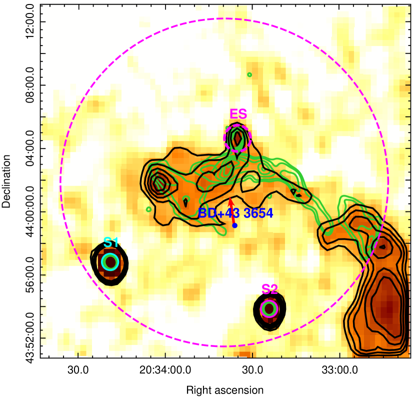
Figure 9: WENSS intensity image of BD+43°3654 at 325 MHz. The full width at half maximum of the beam is $\approx 54^{\prime\prime}\times 77^{\prime\prime}$. The black contour levels are at 44, 54, 64, 74, and 84  mJy beam^-1. We overplot green contours from the intensity map at 3 GHz from Benaglia et al. (2021) at the levels of 1.5, 2, 3, 4, 5, and 6  mJy beam^-1; the dashed circle corresponds to the primary beam of that observation.

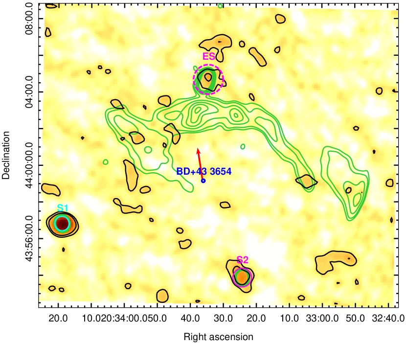
Figure 10: Intensity map of BD+43°3654 at 150 MHz. The beam size is $25^{\prime\prime}\times 25^{\prime\prime}$. The black contour levels are at 10 and 20  mJy beam^-1. We overplot the same contours as in Fig. 9.

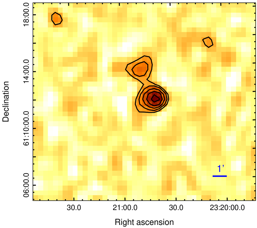
Figure 11: WENSS intensity image of BD+60°2522. The brightest source (south) corresponds to the unresolved emission from the BS of BD+60°2522 together with the dense ionised clumps (Sect. 2.2); the northern arc-shaped source is not from the BS itself, and is also detected in the 4–12 GHz map by Moutzouri et al. (2022). The map has $rms=10$  mJy beam^-1 and an angular resolution of $54^{\prime\prime}\times 62^{\prime\prime}$. Contour levels are at 30, 50, 80, 120, and 170  mJy beam^-1.

Appendix B H_α emission of Vela X-1

The ionised gas in the IL is also responsible for producing the H_α emission from the stellar BS. Thus, this poses an additional constraint to our model that is sensitive only to the width of the IL via the free parameter $\eta_{H}$. We therefore computed the H_α surface brightness map of Vela X-1 and compared it with the observed one from Gvaramadze et al. (2018) to estimate the width of the IL. We calculated the H_α emission adapting the expression given by Gvaramadze et al. (2018) as

$$S_{\alpha}(\theta)\approx 4.3\times 10^{10}\frac{\kappa(\theta)\,{\rm d}V(\theta)}{d^{2}}\;{\rm erg\,s^{-1}\,cm^{-2}},$$ (22)

with d$V(\theta)\propto H_{\rm IL}(\theta)$ the volume of each cell, and

$$\kappa(\theta)=2.85\times 10^{33}\,\left(\frac{T}{{\rm K}}\right)^{-0.9}\left(\frac{n_{e}}{{\rm cm}^{-3}}\right)\,\left(\frac{n_{p}}{{\rm cm}^{-3}}\right).$$ (23)

We finally convolved the synthetic map with a circular beam and divided by the beam area to get a surface brightness map in units of $\mathrm{R}=5.66\times 10^{-18}\leavevmode\nobreak\$erg s^-1 cm^-2 arcsec^-2. Gvaramadze et al. (2018) measured a peak surface brightness of 43 R near the apex of the BS of Vela X-1. To match this value, we needed to set $\eta_{\rm H}\approx 0.1$ (Fig. 12), which implies a significant reduction in the IL.

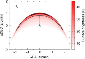
Figure 12: Simulated H_α surface brightness with our model. Contour levels are 20 and 43 R.