An efficient stochastic particle method for high-dimensional nonlinear PDEs

Abstract

Numerical resolution of high-dimensional nonlinear PDEs remains a huge challenge due to the curse of dimensionality. Starting from the weak formulation of the Lawson-Euler scheme, this paper proposes a stochastic particle method (SPM) by tracking the deterministic motion, random jump, resampling and reweighting of particles. Real-valued weighted particles are adopted by SPM to approximate the high-dimensional solution, which automatically adjusts the point distribution to intimate the relevant feature of the solution. A piecewise constant reconstruction with virtual uniform grid is employed to evaluate the nonlinear terms, which fully exploits the intrinsic adaptive characteristic of SPM. Combining both can SPM achieve the goal of adaptive sampling in time. Numerical experiments on the 6-D Allen-Cahn equation and the 7-D Hamiltonian-Jacobi-Bellman equation demonstrate the potential of SPM in solving high-dimensional nonlinear PDEs efficiently while maintaining an acceptable accuracy.

1 Introduction

High-dimensional PDEs have been widely used in modeling complicated physical and social phenomena. Typical examples include the $n$-body Schrödinger equation or the Wigner equation [1], with the dimension $3n$ or $6n$, in describing the many-body quantum world, the Black–Scholes equation for option pricing with the dimension being the number of risky assets [2], the Hamilton–Jacobi–Bellman (HJB) equation in control theory the dimension of which is the number of players [3], and the parametrized family of PDEs arising in inverse problem and uncertainty quantification, where the number of parameters may even be infinite [4]. In contrast to their sound theoretical validation, the notorious curse of dimensionality (CoD) poses a fundamental obstacle to numerical resolution of high-dimensional problems for the cost increases exponentially with the dimensionality.

Up to now, all existing numerical attempts to break CoD often fall into two distinct categories: Grid-based methods and particle-based methods. With the help of high-performance computing platforms, the former have made significant advances towards simulating real 6-D PDEs, e.g., the Boltzmann equation with variable hard sphere kernel [5], the Vlasov equation [6], the Schrödinger equation for two-electron atoms [7], the quantum Wigner-Coulomb system [8] and the Euler-Lagrange equation for icosahedral quasicrystals [9]. However, since the number of basis functions used still explodes with the dimension, it is entirely not trivial to extend them into PDEs in higher dimensions subject to the memory limit of current computers. Particle-based methods that utilize the radial basis functions [10], sophisticated sampling [11, 12] and optimization [13] have also achieved a huge success in solving certain high-dimensional PDEs in engineering and finance, but their performance relies heavily on the low effective dimension underlying the problems [12]. Recently, Deep-learning-based PDE solvers, which are also recognized as particle-based methods [14], have emerged with a rapid development and been applied to solve high-dimensional PDEs in many areas [15, 16, 17]. But there are still some limitations on the ability of the deep neural networks to present a solution with a too complex structure in high dimension [17]. For this reason, the adaptive-sampling-in-time approach, or the active learning, seems to be highly desirable [18].

In this paper, we propose a stochastic particle method (SPM) for solving high-dimensional nonlinear PDEs, e.g., the 7-D HJB equation, which automatically distributes particles relevant to their high-dimensional solutions. A rough idea of using stochastic particles to integrate PDEs dates back to the CFL paper [19] where the boundary value problem of elliptic equations was connected with the random walk problem through a finite difference scheme. Whether a SPM may break CoD has attracted attentions in the recent decade. Several attempts based on the Feynman-Kac formula were proposed, such as the multi-level Monte Carlo method for linear parabolic equations [11], the branching diffusion process algorithm [20] and the multi-level Picard iterative algorithm [21] for semi-linear parabolic equations. However, these methods usually obtain the function value at a prescribed point every run and there still remain some key issues to be further studied. For example, the exponential growth of particles in the branching diffusion process algorithm result in a short-time simulation, and the Lipschitz constant of nonlinear terms is restricted to be small in the multi-level Picard iteration. It is more important to note that the Feynman-Kac formula expresses the solution as the expectation of a positive weighted particle system. What if particles possess different charges? This will make the mathematical tools of probability theory almost unusable [22]. Techniques from optimal transport may be helpful in studying evolution PDEs with sign-changing solutions, like the Wasserstein distance for signed measures [23] and the Kantorovitch Rubinstein duality [24]. Motivated by the CFL paper [19], which obtains stochastic particle interpretation directly from the numerical schemes rather than from the PDEs, this work proposes an alternative way to obtain SPM for high-dimensional nonlinear PDEs with sign-changing solutions by starting from the corresponding Lawson-Euler time discretization [25].

When dealing with CoD, the accuracy of an efficient numerical method can be expected at current stage is only half order, like the Monte Carlo with convergence rate $\mathcal{O}(N^{-1/2})$ and $N$ being the sample size, rather than a high order one. In keeping with such spirit, we choose the Lawson-Euler scheme which linearizes the nonlinear terms using the solutions at the previous time step and thus only has first-order accuracy in time. After that, just like most traditional numerical methods, we propose to use the weak formulation for obtaining stochastic particle representation in high-dimensional space, the usefulness of which can be twofold. First, it allows us to conveniently extract required information from the high-dimensional unknown functions. By plugging different test functions into the weak formulation, it is able to figure out the desired information of the solutions more than the function value at a fixed point. Second, it appears as a high-dimensional integral that depends on time and the underlying PDE establishes a bridge in the time direction. That is, SPM can be seen as using the Monte Carlo to approximate the time-dependent integral, and simulates the evolution of the PDE through particle motion and weight update and so on. This is the key point to automatically adjust the particles to intimate the feature of high-dimensional solutions, thereby achieving the goal of adaptive sampling. It should be pointed out that, the proposed SPM does not depend on the Feynman-Kac formula.

Starting from the weak formulation of the Lawson-Euler scheme, SPM uses real-valued weighted particles to approximate the high-dimensional solution in the weak sense. It tracks the deterministic motion, random jump, resampling and reweighting of particles. To reduce the cost of reconstructing the solution values via weighted particles and in accordance with the first-order accuracy of the Lawson-Euler scheme, it suggests to adopt a uniform piecewise constant reconstruction with virtual uniform grid (VUG) by fully taking advantage of the high adaptivity of stochastic particles. It should be noted that, finding the optimal piecewise constant reconstruction is an NP-hard problem [26] with high computational complexity. SPM is fully adaptive in nature and easy to parallelize. Using the distributed parallel technology via Message Passing Interface (MPI), it solves the 6-D Allen-Cahn equation and the 7-D HJB equation efficiently while maintaining a reasonable error tolerance, and the accuracy can be systematically improved by increasing the number of particles.

The rest of this paper is organized as follows. In Section 2, we introduce the theory of stochastic particle method. Section 3 presents more implementation details. Some 1-D benchmark tests are conducted in Section 4. Section 5 and Section 6 show numerical experiments for solving the 6-D Allen-Cahn equation and the 7-D HJB equation, respectively. The paper is concluded in Section 7 with a few remarks.

2 The stochastic particle method

Consider nonlinear PDEs of the following form,

$$\frac{\partial}{\partial t}u(\bm{x},t) =\mathcal{L}u(\bm{x},t)+f(t,\bm{x},u,\nabla u,\nabla^{2}u,\dots),\quad\bm{x}\in\mathbb{R}^{d},~{}t>0,$$ (1)

$$u(\bm{x},0) =u_{0}(\bm{x}),\quad\bm{x}\in\mathbb{R}^{d},$$

where $\mathcal{L}$ represents the linear operator, $f(t,\bm{x},u,\nabla u,\nabla^{2}u,\dots)$ gives the nonlinear term, and the initial data $u_{0}(\bm{x})\in L^{2}(\mathbb{R}^{d})$.

Example 2.1.

$\mathcal{L}=\boldsymbol{b}\cdot\nabla$ is the gradient operator, where $\boldsymbol{b}\in\mathbb{R}^{d}$ is a constant vector.

Example 2.2.

$\mathcal{L}=c\Delta$ is the Laplace operator, where $c>0$ is a constant.

Example 2.3.

For the Allen-Cahn equation, $f(t,\bm{x},u,\nabla u,\dots)=u(\bm{x},t)-(u(\bm{x},t))^{3}$.

Example 2.4.

For a special kind of HJB equation, $f(t,\bm{x},u,\nabla u,\dots)=\lVert\nabla u(\bm{x},t)\rVert_{2}^{2}$, where $\lVert\cdot\rVert_{2}$ denotes the standard $L^{2}$-norm.

Substituting the change of variable $v(\bm{x},t):=\mathbbm{e}^{-t\mathcal{L}}u(\bm{x},t)$ into Eq. (1) yields

$$\frac{\partial}{\partial t}v(\bm{x},t)=\mathbbm{e}^{-t\mathcal{L}}f(t,\bm{x},\mathbbm{e}^{t\mathcal{L}}v,\nabla\mathbbm{e}^{t\mathcal{L}}v,\nabla^{2}\mathbbm{e}^{t\mathcal{L}}v,\dots),$$ (2)

which can be readily integrated by any ODE integrator. In view of simplicity and the positivity-preserving property, the first-order time discretization turns out to be more appealing [27]. Accordingly, we apply the explicit Euler scheme to Eq. (2):

$$v(\bm{x},t+\tau)\approx v(\bm{x},t)+\tau\mathbbm{e}^{-t\mathcal{L}}f(t,\bm{x},\mathbbm{e}^{t\mathcal{L}}v,\nabla\mathbbm{e}^{t\mathcal{L}}v,\nabla^{2}\mathbbm{e}^{t\mathcal{L}}v,\dots),$$

then back to $u(\bm{x},t)$, we have the so-called Lawson-Euler scheme [25]:

$$U_{m+1}(\bm{x})=\mathbbm{e}^{\tau\mathcal{L}}\left(U_{m}(\bm{x})+\tau f(t_{m},\bm{x},U_{m},\nabla U_{m},\dots)\right),$$ (3)

where $\tau$ is the time step and $U_{m}(\bm{x})$ denotes the numerical solution at $t_{m}=m\tau$ (we have $U_{0}(\bm{x})\equiv u_{0}(\bm{x})$ by default). Hereafter, we will take the Lawson-Euler scheme (3) as an example to show how SPM can be combined with existing time discretization methods.

We use $N$ stochastic particles to evolve Eq. (3) in the weak sense. The $i$-th particle carries two key quantities: Location $\bm{x}_{i}\in\mathbb{R}^{d}$ and weight $w_{i}\in\mathbb{R}$. All particles at $t_{m}$ form a weighted point distribution

$$X_{t_{m}}=\frac{1}{N}\sum_{i=1}^{N}w_{i}(t_{m})\delta_{\bm{x}_{i}(t_{m})},$$ (4)

which can be used to approximate $U_{m}(\bm{x})$ in the weak sense

$$\langle\varphi,U_{m}\rangle\approx\langle\varphi,X_{t_{m}}\rangle=\frac{1}{N}\sum_{i=1}^{N}w_{i}(t_{m})\varphi(\bm{x}_{i}(t_{m})),$$ (5)

where the standard inner product $\langle f,g\rangle=\int_{\mathbb{R}^{d}}f(\bm{x})g(\bm{x})\textup{d}\bm{x}$ is adopted, and the test function $\varphi\in\mathbb{H}^{2}(\mathbb{R}^{d})$ has a compact support in $\mathbb{R}^{d}$. Various information of $U_{m}(\bm{x})$ can be figured out by choosing different test function $\varphi(\bm{x})$. The weak formulation (5) defines a high-dimensional integral that depends on time.

When the particle location $\bm{x}_{i}$ follows the instrumental distribution $p(\bm{x})$ at time $t_{m}$, according to

$$\langle\varphi,U_{m}\rangle=\int_{\mathbb{R}^{d}}\varphi(\bm{x})\frac{U_{m}(\bm{x})}{p(\bm{x})}p(\bm{x})\textup{d}\bm{x}\approx\frac{1}{N}\sum_{i=1}^{N}\varphi(\bm{x}_{i})\frac{U_{m}(\bm{x}_{i})}{p(\bm{x}_{i})}=\frac{1}{N}\sum_{i=1}^{N}\varphi(\bm{x}_{i})w_{i}=\langle\varphi,X_{t_{m}}\rangle,$$ (6)

we should let the weight $w_{i}={U_{m}(\bm{x}_{i})}/{p(\bm{x}_{i})}$. No matter what $p(\bm{x})$ we have chosen, the expectation of $\langle\varphi,X_{t_{m}}\rangle$ is always $\langle\varphi,U_{m}\rangle$, but the variance may be significantly different. The idea of importance sampling [28] can be used to reduce the variance. From

$$Var\left(\frac{\varphi U_{m}}{p}\right)=\int_{\mathbb{R}^{d}}\left[\varphi(\bm{x})\frac{U_{m}(\bm{x})}{p(\bm{x})}\right]^{2}p(\bm{x})\textup{d}\bm{x}-(\langle\varphi,U_{m}\rangle)^{2}=\int_{\mathbb{R}^{d}}\frac{(\varphi(\bm{x})U_{m}(\bm{x}))^{2}}{p(\bm{x})}\textup{d}\bm{x}-(\langle\varphi,U_{m}\rangle)^{2},$$ (7)

we have the most ideal distribution $p^{*}(\bm{x})=\varphi(\bm{x})U_{m}(\bm{x})/\langle\varphi,U_{m}\rangle$ and thus $Var\left({\varphi U_{m}}/{p}\right)=0$ providing that $\varphi(\bm{x})U_{m}(\bm{x})$ is non-negative. However, this is actually impossible because: (a) the prerequisite for obtaining $p^{*}(\bm{x})$ is that we already know $\langle\varphi,U_{m}\rangle$ which is our original mission, (b) $\varphi(\bm{x})$ and $U_{m}(\bm{x})$ considered in our work are real-valued function, and (c) $\varphi(\bm{x})$ is not predetermined and we use different $\varphi(\bm{x})$ to extract different information of $U_{m}(\bm{x})$. Nevertheless, the idea of importance sampling can still guide us to adjust the distribution of particle location to maintain a small variance. More specifically, we are going to use ${|U_{m}(\bm{x})|}/{\int_{\mathbb{R}^{d}}|U_{m}(\bm{x})|\textup{d}\bm{x}}$ as a feasible alternative to $p^{*}(\bm{x})$. At the initial stage, the particle location $\bm{x}_{i}(0)$ can be sampled from $p(\bm{x})={|U_{0}(\bm{x})|}/{\int_{\mathbb{R}^{d}}|U_{0}(\bm{x})|\textup{d}\bm{x}}$, then assign the weights $w_{i}(0)={U_{0}(\bm{x}_{i}(0))}/{p(\bm{x}_{i}(0))}$ accordingly. Afterwards, the Lawson-Euler scheme (3) establishes the relationship between $U_{m}(\bm{x})$ and $U_{m+1}(\bm{x})$. It can guide particle motion and weight update.

In particular, Section 2.1 gives two evolution strategies of weighted particle system, a preliminary strategy and an improved strategy, denoted as Strategy A and Strategy B, respectively. The derivation of Strategy A is more straightforward, but it poses some restrictions on the nonlinear term $f(t_{m},\bm{x},U_{m},\nabla U_{m},\dots)$ while the importance sampling principle is not fully respected. On the contrary, Strategy B can deal with general nonlinear term and respects the importance sampling principle more.

2.1 Particle motion and weight update

To begin with, we introduce Strategy A under the Assumption 2.1.

Assumption 2.1.

$U_{m}(\bm{x})=0$ implies $f(t_{m},\bm{x},U_{m},\nabla U_{m},\dots)=0$.

From Eq. (3), we get

$$\langle\varphi,U_{m+1}\rangle=\langle\mathbbm{e}^{\tau\mathcal{L}^{*}}\varphi,\left(1+\tau\hat{f}(t_{m},\bm{x},U_{m},\nabla U_{m},\dots)\right)U_{m}\rangle,$$ (8)

where $\mathcal{L}^{\ast}$ denotes the adjoint operator of $\mathcal{L}$ defined on $\mathbb{H}^{2}(\mathbb{R}^{d})$, and

$$\hat{f}(t_{m},\bm{x},U_{m},\nabla U_{m},\dots)=\left\{\begin{aligned} &\frac{f(t_{m},\bm{x},U_{m},\nabla U_{m},\dots)}{U_{m}},&\quad\bm{x}\in\textup{supp}\,U_{m},\\ &0,&\quad\bm{x}\notin\textup{supp}\,U_{m}.\end{aligned}\right.$$ (9)

For Example 2.3, the nonlinear term of Allen-Cahn equation $f(t_{m},\bm{x},U_{m},\nabla U_{m},\dots)=U_{m}(\bm{x})-\left(U_{m}(\bm{x})\right)^{3}=0$ when $U_{m}(\bm{x})=0$ and Assumption 2.1 is satisfied. In this case,

$$\hat{f}(t,\bm{x},U_{m}(\bm{x}),\nabla U_{m}(\bm{x}),\dots)=\left\{\begin{aligned} &1-(U_{m}(\bm{x}))^{2},&\quad\bm{x}\in\textup{supp}\,U_{m}(\bm{x}),\\ &0,&\quad\bm{x}\notin\textup{supp}\,U_{m}(\bm{x}).\end{aligned}\right.$$ (10)

When $U_{m}(\bm{x})$ in Eq. (8) is approximated by the weighted point distribution (4), the dynamics of particle estimator reads that

$$\langle\varphi,U_{m+1}\rangle =\frac{1}{N}\sum_{i=1}^{N}w_{i}(t_{m})(1+\tau\hat{f}(t_{m},\bm{x}_{i}(t_{m}),U_{m},\nabla U_{m},\dots))\mathbbm{e}^{\tau\mathcal{L}^{*}}\varphi(\bm{x}_{i}(t_{m}))$$ (11)

$$=\frac{1}{N}\sum_{i=1}^{N}w_{i}(t_{m+1})\mathbb{E}\varphi(\bm{x}_{i}(t_{m+1})),$$

where we define

$$\mathbb{E}\varphi(\bm{x}_{i}(t_{m+1}))=\mathbbm{e}^{\tau\mathcal{L}^{*}}\varphi(\bm{x}_{i}(t_{m})),$$ (12)

$$w_{i}(t_{m+1})=w_{i}(t_{m})\left(1+\tau\hat{f}(t_{m},\bm{x}_{i}(t_{m}),U_{m},\nabla U_{m},\dots)\right).$$ (13)

In other words, we may directly update the particle weights according to Eq. (13) where the nonlinear term enters into, and the dynamics of particle trajectories is updated as

$$\bm{x}_{i}(t_{m})\xrightarrow{\mathbbm{e}^{\tau\mathcal{L}^{*}}}\bm{x}_{i}(t_{m+1}),$$ (14)

which is governed by the linear adjoint operator $\mathcal{L}^{*}$. The implementation of Eq. (14) reflects the action of $\mathcal{L}^{*}$ and corresponds to solving the linear equation

$$\frac{\partial}{\partial t}g(\bm{x},t)=\mathcal{L}^{\ast}g(\bm{x},t),\quad g(\bm{x},0)=\varphi(\bm{x}).$$ (15)

For Example 2.1, we have $\mathcal{L}^{\ast}=-\boldsymbol{b}\cdot\nabla$, and then the analytical solution of Eq. (15) is

$$g(\boldsymbol{x},t)=\varphi(\boldsymbol{x}-\boldsymbol{b}t),$$

which implies that

$$\bm{x}_{i}(t_{m+1})=\bm{x}_{i}(t_{m})-\boldsymbol{b}\tau,$$

i.e., a kind of linear advection along the characteristic line.

For Example 2.2, we have $\mathcal{L}^{\ast}=c\Delta$, and then the analytical solution of Eq. (15) has the closed form

$$g(\boldsymbol{x},t)=\int_{\mathbb{R}^{d}}\frac{1}{(2\pi)^{d/2}\sqrt{|\Sigma|}}\mathbbm{e}^{-\frac{1}{2}\boldsymbol{y}^{T}\Sigma^{-1}\boldsymbol{y}}\varphi(\boldsymbol{x}-\boldsymbol{y})\textup{d}\boldsymbol{y},\quad\Sigma=2ctI,$$

with $I$ being the identity matrix of order $d$. It has a transparent probability interpretation $\mathrm{e}^{tc\Delta}\varphi(\boldsymbol{x})=\mathbb{E}\left[\varphi(\boldsymbol{x}-\boldsymbol{y})\right]$, where $\boldsymbol{y}\sim\mathcal{N}(\boldsymbol{0},\Sigma)$. To be more specific, it corresponds to the Brownian motion

$$\boldsymbol{x}_{i}(t_{m+1})=\boldsymbol{x}_{i}(t_{m})-\boldsymbol{y},\;\;\;\text{with}\;\;\;\boldsymbol{y}\sim\mathcal{N}(\boldsymbol{0},2c\tau I).$$

In fact, for arbitrary linear operator $\mathcal{L}$, the rules of motions can be designed via its kernel representation. For instance, the pseudo-differential operator in the Wigner equation has the probability interpretation of branching random walk based on the Neumann series expansion [29].

Next, we introduce Strategy B which can handle a general nonlinear term and does not need Assumption 2.1. From Eq. (3), we obtain

$$\langle\varphi,U_{m+1}\rangle =\langle\mathbbm{e}^{\tau\mathcal{L}^{*}}\varphi,U_{m}+\tau f(t_{m},\bm{x},U_{m},\nabla U_{m},\dots)\rangle$$ (16)

$$=\left\langle\mathbbm{e}^{\tau\mathcal{L}^{*}}\varphi,\frac{[U_{m}+\tau f(t_{m},\bm{x},U_{m},\nabla U_{m},\dots)]Z}{|U_{m}+\tau f(t_{m},\bm{x},U_{m},\nabla U_{m},\dots)|}\cdot\frac{|U_{m}+\tau f(t_{m},\bm{x},U_{m},\nabla U_{m},\dots)|}{Z}\right\rangle$$

$$\approx\frac{1}{N}\sum_{i=1}^{N}\frac{[U_{m}(\widetilde{\bm{x}_{i}}(t_{m}))+\tau f(t_{m},\widetilde{\bm{x}_{i}}(t_{m}),U_{m},\nabla U_{m},\dots)]Z}{|U_{m}(\widetilde{\bm{x}_{i}}(t_{m}))+\tau f(t_{m},\widetilde{\bm{x}_{i}}(t_{m}),U_{m},\nabla U_{m},\dots)|}\mathbbm{e}^{\tau\mathcal{L}^{*}}\varphi(\widetilde{\bm{x}_{i}}(t_{m}))$$

$$=\frac{1}{N}\sum_{i=1}^{N}w_{i}(t_{m+1})\mathbb{E}\varphi(\bm{x}_{i}(t_{m+1})),$$

where we define

$$\mathbb{E}\varphi(\bm{x}_{i}(t_{m+1}))=\mathbbm{e}^{\tau\mathcal{L}^{*}}\varphi(\widetilde{\bm{x}_{i}}(t_{m})),$$ (17)

$$w_{i}(t_{m+1})=\frac{U_{m}(\widetilde{\bm{x}_{i}}(t_{m}))+\tau f(t_{m},\widetilde{\bm{x}_{i}}(t_{m}),U_{m},\nabla U_{m},\dots)Z}{|U_{m}(\widetilde{\bm{x}_{i}}(t_{m}))+\tau f(t_{m},\widetilde{\bm{x}_{i}}(t_{m}),U_{m},\nabla U_{m},\dots)|},$$ (18)

and $\widetilde{\bm{x}_{i}}(t_{m})$ is re-sampled from the density $|U_{m}(\bm{x})+\tau f(t_{m},\bm{x},U_{m},\nabla U_{m},\dots)|/Z$,

$$\widetilde{\bm{x}_{i}}(t_{m})\sim\frac{1}{Z}|U_{m}(\bm{x})+\tau f(t_{m},\bm{x},U_{m},\nabla U_{m},\dots)|,\quad Z=\int_{\mathbb{R}^{d}}|U_{m}(\bm{x})+\tau f(t_{m},\bm{x},U_{m},\nabla U_{m},\dots)|\textup{d}\bm{x}.$$ (19)

Unlike the location update in Eq. (14) of Strategy A, the dynamics of particle trajectories in Strategy B is

$$\bm{x}_{i}(t_{m})\xrightarrow{\text{relocating}}\widetilde{\bm{x}_{i}}(t_{m})\xrightarrow{\mathbbm{e}^{\tau\mathcal{L}^{*}}}\bm{x}_{i}(t_{m+1}),$$ (20)

and an extra step of the relocating technique given in Eq. (19) is inserted when updating the location from $\bm{x}_{i}(t_{m})$ to $\bm{x}_{i}(t_{m+1})$. After that, we assign the particle weight according to Eq. (18).

For Strategy A, the change of particle location is only affected by the linear part as displayed in Eq. (12), set against the fact that the evolution of Eq. (3) results from the joint action of linear and nonlinear terms. That is, after a period of evolution, the distribution of particle location in Strategy A may not match the shape of solution well (see Figure 3), thereby leading to an increase in stochastic variances of Eq. (6). Thanks to the relocating technique in Eq. (19), Strategy B actively adjusts the particle location to obey $|U_{m}(\bm{x})+\tau f(t_{m},\bm{x},U_{m},\nabla U_{m},\dots)|/Z$, a first-order approximation to ${|U_{m+1}(\bm{x})|}/{\int_{\mathbb{R}^{d}}|U_{m+1}(\bm{x})|\textup{d}\bm{x}}$ as shown in the following,

$$\lvert U_{m+1}(\bm{x})\rvert =\lvert\mathbbm{e}^{\tau\mathcal{L}}\left(U_{m}(\bm{x})+\tau f(t_{m},\bm{x},U_{m},\nabla U_{m},\dots)\right)\rvert$$ (21)

$$=\left|\left(1+\tau\mathcal{L}+\frac{\left(\tau\mathcal{L}\right)^{2}}{2}+\cdots\right)\left(U_{m}(\bm{x})+\tau f(t_{m},\bm{x},U_{m},\nabla U_{m},\dots)\right)\right|$$

$$=\lvert U_{m}(\bm{x})+\tau f(t_{m},\bm{x},U_{m},\nabla U_{m},\dots)\rvert+\mathcal{O}(\tau),$$

which also agrees with the order of the Lawson-Euler scheme (3). When the evolution is performed in a short time interval, the difference between the two strategies may be not significant. But in long-time simulations, the relocating technique in Eq. (19), making the particle location close to the shape of $U_{m}(\bm{x})$, is crucial, with which the particle weight is more uniform and the variance is smaller when calculating Eq. (6). This can be readily verified through benchmark tests in Section 4.

2.2 Piecewise constant reconstruction from weighted point distribution

According to the dynamics of particle estimator in Eqs. (13) and (18), we need to know the values of $U_{m}(\bm{x})$ and $f(t,\bm{x},U_{m}(\bm{x}),\nabla U_{m}(\bm{x}),\dots)$ for both strategies. It requires to approximate $U_{m}(\bm{x})$, $\nabla U_{m}(\bm{x})$, $\nabla^{2}U_{m}(\bm{x}),\dots$ using the weighted point distribution (4). Generally speaking, when $U_{m}(\bm{x})$ is sufficiently smooth, those quantities like $\nabla U_{m}(\bm{x})$, $\nabla^{2}U_{m}(\bm{x}),\dots$ can be approximated by corresponding difference quotients, so we just need to focus on how to compute $U_{m}(\bm{x})$. There exist several numerical techniques for constructing function values from point cloud, such as the piecewise constant approximation [30], the Fourier series approximation [31] and the sequential function approximation [32, 33]. In this work, we adopt the first-order piecewise constant approximation to obtain $U_{m}(\bm{x})$.

Let $\Omega=\left[l,r\right]^{d}\subset\mathbb{R}^{d}$ be the computational domain containing all particles. It can be decomposed into

$$\Omega=\left[l,r\right]^{d}=\bigcup_{k=1}^{K}Q_{k},$$ (22)

so that $U_{m}(\bm{x})$ can be approximated by constant in each sub-domain $Q_{k}$ (usually a hypercube with the size length of $h_{k}$). The discussion on how to achieve such decomposition is left to Section 3. Suppose location $\boldsymbol{x}$ at which the function value needs to be evaluated falls into the sub-domain $Q_{k}$, then in a similar way to Eq. (5), we may have

$$U_{m}(\bm{x})\approx\frac{1}{\mu(Q_{k})}\int_{Q_{k}}U_{m}(\bm{y})\textup{d}\boldsymbol{y}\approx\frac{1}{N}\sum_{i=1}^{N}\frac{w_{i}(t_{m})\mathbbm{1}_{Q_{k}}(\bm{x}_{i}(t_{m}))}{\mu(Q_{k})},$$ (23)

where $\mu(Q_{k})$ gives the Lebesgue measure of $Q_{k}$. In fact, we are able to obtain the second approximation in Eq. (23) by taking $\varphi(\bm{x})$ as the indicator function $\mathbbm{1}_{Q_{k}}(\bm{x})$ in Eq. (5).

The nonlinear term in Example 2.4 contains gradient operator and we adopt the center difference quotient to approximate the derivative in the $j$-th coordinate,

$$\frac{\partial}{\partial x_{j}}U_{m}(\bm{x})\approx\frac{U_{m}(\bm{x}+\Delta x_{j}\bm{e}_{j})-U_{m}(\bm{x}-\Delta x_{j}\bm{e}_{j})}{2\Delta x_{j}},$$ (24)

where the unit vector $\bm{e}_{j}$ denotes the direction of the $j$-th coordinate and $\Delta x_{j}$ the corresponding spacing.

Up to this point, we have delineated the mathematical description of SPM and are also able to classify its errors into three levels as follows,

• Spatial discretization: The piecewise constant reconstruction (23) introduces a spatial approximation error of $\mathcal{O}(h_{k})$;

• Time discretization: The Lawson-Euler scheme (3) introduces a time discretization error of $\mathcal{O}(\tau)$;

• Monte Carlo sampling: The stochastic particle approximation (5) introduces a sampling error of $\mathcal{O}(N^{-1/2})$.

Generally speaking, the sampling error dominates. We would like to remark on other kinds of time discretization rather than the Lawson-Euler scheme (3) including, for example, the exponential time differencing scheme [34] and the Strang splitting scheme [35]. The Lawson-Euler scheme may be more stable than the exponential time differencing scheme [36], though they are both of the first order accuracy. Besides, considering the time discretization error does not dominate the errors of SPM, even the first-order accurate Lawson-Euler scheme may allow a large time step without recourse to the second-order accurate Strang splitting.

3 Implementation details and cost analysis

We have already had two strategies for particle motion and weight update, but there still remain some implementation details, such as how to achieve the decomposition (22) and how to sample $\widetilde{\bm{x}_{i}}(t_{m})$ in (19).

3.1 Piecewise constant reconstruction and virtual uniform grid (VUG)

An optimal way for piecewise constant reconstruction can be implemented by solving

$$\inf\limits_{Q_{k}}\sup\limits_{\varphi\in D(\varphi)}\left|\int_{\mathbb{R}^{d}}\varphi(\bm{x})\sum\limits_{Q_{k}}\left(\sum_{i=1}^{N}\frac{w_{i}\mathbbm{1}_{Q_{k}}(\bm{x}_{i}(t_{m}))}{N\mu\left({Q_{k}}\right)}\right)\mathbbm{1}_{Q_{k}}(\bm{x})\textup{d}\bm{x}-\frac{1}{N}\sum_{i=1}^{N}w_{i}\varphi(\bm{x}_{i}(t_{m}))\right|,$$ (25)

where $D(\varphi)=\{\varphi\in\mathbb{H}^{2}(\mathbb{R}^{d}):\varphi\text{ has bounded variation}\}$. Along this line, an adaptive sequential partition strategy based on the star discrepancy, which measures the degree of uniformity, was proposed in [26], where the decomposition is sequentially refined until the star discrepancy of particle locations inside each $Q_{k}$ is less than a prescribed threshold. However, the complexity of calculating the star discrepancy is NP-hard [37] and one has to deal with a significant computational cost when $N$ is large. Instead, considering the highly adaptive nature of stochastic particles, this work chooses a “uniform partitioning” as an approximation to the problem (25) without storing the full tensor girds, and the resulting method is termed “virtual uniform grid” (VUG). More specifically, during the $m$-th step, the particle location is close to ${|U_{m}(\bm{x})|}/{\int_{\mathbb{R}^{d}}|U_{m}(\bm{x})|\textup{d}\bm{x}}$ and VUG does not store the grids inside areas where ${|U_{m}(\bm{x})|}/{\int_{\mathbb{R}^{d}}|U_{m}(\bm{x})|\textup{d}\bm{x}}$ vanishes, thereby avoiding unnecessary storage as much as possible. Given a uniform decomposition as shown in Eq. (22), each $Q_{k}$ is a hypercube with the same side length, denoted by $h$, and thus VUG has a storage cost of around $\alpha\left(\frac{r-l}{h}\right)^{d}$, where $\alpha\in(0,1)$ is the ratio of the stored grids to the full ones. Figure 1 gives an illustration where only 7 grids containing particles in all 25 grids should be stored, namely $\alpha=\frac{7}{25}$. In general, such ratio $\alpha$ depends on the shape of unknown functions, and generally decreases as the dimension increases, which can be readily verified, for instance, through the numerical experiments in Example 3.1.

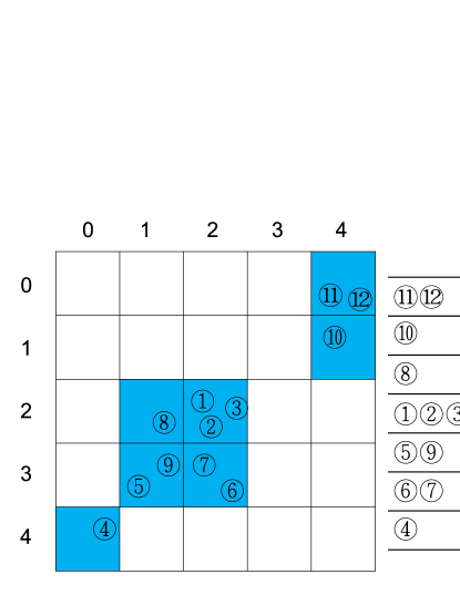
Figure 1: VUG: Only blue grids, containing the particles, are stored, and the corresponding grid coordinates for all particles are presented on the right.

Example 3.1.

Consider a sign-changing function

$$p^{\text{ref}}(\bm{x})=\prod_{j=1}^{d}f_{15,5}(x_{j})-\prod_{j=1}^{d}f_{10,10}(x_{j})+\prod_{j=1}^{d}f_{5,15}(x_{j})$$ (26)

with $f_{\alpha,\beta}(x)$ being the beta distribution density

$$f_{\alpha,\beta}(x)=\frac{\Gamma(\alpha+\beta)}{\Gamma(\alpha)\Gamma(\beta)}x^{\alpha-1}(1-x)^{\beta-1},\quad 0\leq x\leq 1.$$ (27)

One can sampling from $p^{\text{ref}}(\bm{x})$ and do piecewise constant reconstruction through VUG to get a numerical solution $p^{\text{num}}(\bm{x})$. Table 1 shows the numerical results of VUG in different dimensions $d$ for different sample sizes $N$ where the relative $L^{2}$ error

$$\mathcal{E}_{2}[p]=\frac{\lVert p^{\text{num}}(\bm{x})-p^{\text{ref}}(\bm{x})\rVert_{2}}{\lVert p^{\text{ref}}(\bm{x})\rVert_{2}}$$ (28)

is adopted to investigate the accuracy. It can be easily observed there that the error $\mathcal{E}_{2}[p]$ decreases as the sample size $N$ increases for fixed $d$, and the ratio $\alpha$ always decreases as the dimension $d$ increases.

Table 1: Example 3.1: The relative $L^{2}$ error and the ratio $\alpha$ when using VUG to do piecewise constant reconstruction in 4-D to 7-D with a fixed side length $h=0.0625$. # VUG in the fourth column represents the number of virtual uniform grids, the $\left(\frac{r-l}{h}\right)^{d}$ in the fifth column represents the number of full grids. Overall, the ratio $\alpha$ decreases as the dimension $d$ increases.

$d$	$N$	$\mathcal{E}_{2}[p]$	# VUG	$\left(\frac{r-l}{h}\right)^{d}$	$\alpha$
	$1\times 10^{6}$	0.0693	$1.86\times 10^{4}$		0.283
4	$2\times 10^{6}$	0.0573	$2.09\times 10^{4}$	$6.55\times 10^{4}$	0.318
	$4\times 10^{6}$	0.0495	$2.31\times 10^{4}$		0.353
	$1\times 10^{7}$	0.0657	$1.75\times 10^{5}$		0.166
5	$2\times 10^{7}$	0.0584	$2.01\times 10^{5}$	$1.05\times 10^{6}$	0.191
	$4\times 10^{7}$	0.0543	$2.29\times 10^{5}$		0.218
	$4\times 10^{7}$	0.0777	$1.26\times 10^{6}$		0.075
6	$8\times 10^{7}$	0.0691	$1.52\times 10^{6}$	$1.68\times 10^{7}$	0.091
	$1.6\times 10^{8}$	0.0641	$1.80\times 10^{6}$		0.107
	$1\times 10^{8}$	0.1001	$7.00\times 10^{6}$		0.026
7	$2\times 10^{8}$	0.0861	$8.94\times 10^{6}$	$2.68\times 10^{8}$	0.033
	$4\times 10^{8}$	0.0776	$1.12\times 10^{7}$		0.041

The uniform side length $h$ of hypercubes in the decomposition (22) introduces an asymptotic error of $\mathcal{O}(h)$ for the piecewise constant reconstruction through VUG [38], and thus a large $h$ is not preferred. For Example 3.1, such asymptotic error becomes more evident for $h>0.1$, see Figure 2. However, too small $h$ should NOT be suggested due to the notorious overfitting problem [31, 39], which results in a significant statistical error for the number of grids exceeds the sample size and few particles fall within the same grid. This is also verified in Figure 2: When $h<0.04$, the effective sample size in a grid becomes extremely small and leads to an augmentation of statistical error. A practical way to choose an appropriate $h$ may be as follows. We may take a relatively large $h$ first, and then gradually reduce it until the relative $L^{2}$ error $\mathcal{E}_{2}[p]$ does not diminish with the decrease of $h$.

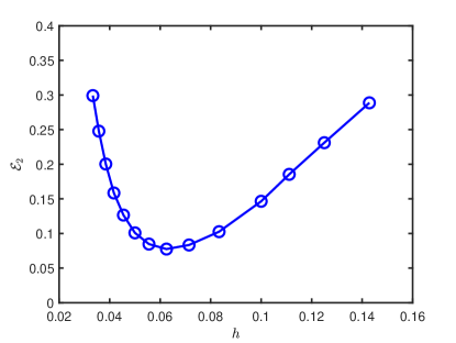
Figure 2: Example 3.1: The relative $L^{2}$ error $\mathcal{E}_{2}[p]$ against the side length $h$ for $d=6$ and $N=4\times 10^{7}$.

In practice, VUG dynamically allocates the memory according to the particle locations at each time step, whereas all the memory is usually allocated in advance for the full tensor grids. Within our C++ implementation, the data structure “map” is adopted to map the grid coordinates in struct type to piecewise constants in double type. Specifically, we need to maintain two “map” data structures: $\mathcal{M}_{1}$ records the piecewise constant approximation to the unknown function and $\mathcal{M}_{2}$ the piecewise constant approximation to the nonlinear term. Algorithm 1 presents the pseudo-code of SPM with VUG and Algorithm 2 details the updating $\mathcal{M}_{1}$ for an incoming new particle.

Algorithm 1 Stochastic particle method with virtual uniform grid

Input: The computational domain $\left[l,r\right]^{d}$, the side length of hypercube $h$, the final time $T$, the time step $\tau$, the initial data $u_{0}(\bm{x})$, the linear operator $\mathcal{L}$ and the nonlinear term $f(t,\bm{x},u,\nabla u,\nabla^{2}u,\dots)$.
  Output: The numerical solution to nonlinear PDE (1) at the final time.

1:Allocate two empty map $\mathcal{M}_{1}$ and $\mathcal{M}_{2}$;

2:for $m=0:\frac{T-\tau}{\tau}$ do

3:     Clear $\mathcal{M}_{1}$;

4:     if Strategy A then

5:         for $i=1:N$ do

6:              if $m=0$ then

7:                  Sample $\bm{x}_{i}$ from $p(\bm{x})=\frac{|U_{0}(\bm{x})|}{\int_{\mathbb{R}^{d}}|U_{0}(\bm{x})|\textup{d}\bm{x}}$;

8:                  $w_{i}\leftarrow\frac{U_{0}(\bm{x}_{i})}{{p(\bm{x}_{i})}}$;

9:              end if

10:              Update $w_{i}$ according to (13);

11:              Move particle according to $\mathcal{L}^{*}$ (the adjoint operator of $\mathcal{L}$);

12:              Update $\mathcal{M}_{1}$ according to $\bm{x}_{i}$ and $w_{i}$;

13:         end for

14:         Clear $\mathcal{M}_{2}$;

15:         Compute $\hat{f}(t_{m+1},\bm{x},U_{m+1},\nabla U_{m+1},\dots)$ and construct $\mathcal{M}_{2}$ based on $\mathcal{M}_{1}$;

16:     else if Strategy B then

17:         for ${i=1:N}$ do

18:              Sample $\bm{x}_{i}$ from ${p(\bm{x})}=\frac{|U_{m}(\bm{x})+\tau f(t_{m},\bm{x},U_{m},\nabla U_{m},\dots)|}{\int_{\mathbb{R}^{d}}|U_{m}(\bm{x})+\tau f(t_{m},\bm{x},U_{m},\nabla U_{m},\dots)|\textup{d}\bm{x}}$;

19:              $w_{i}\leftarrow\frac{U_{m}(\bm{x}_{i})+\tau f(t_{m},\bm{x}_{i},U_{m},\nabla U_{m},\dots)}{{p(\bm{x}_{i})}}$;

20:              Move particle according to $\mathcal{L}^{*}$;

21:              Update $\mathcal{M}_{1}$ according to $\bm{x}_{i}$ and $w_{i}$;

22:         end for

23:         Clear $\mathcal{M}_{2}$;

24:         Compute $U_{m+1}(\bm{x})+\tau f(t_{m+1},\bm{x},U_{m+1},\nabla U_{m+1},\dots)$ and construct $\mathcal{M}_{2}$ based on $\mathcal{M}_{1}$;

25:         Compute $\int_{\mathbb{R}^{d}}|U_{m+1}(\bm{x})+\tau f(t_{m+1},\bm{x},U_{m+1},\nabla U_{m+1},\dots)|\textup{d}\bm{x}$;

26:     end if

27:end for

Algorithm 2 Update piecewise constant approximation $\mathcal{M}_{1}$ according to a new particle

Input: An unupdated $\mathcal{M}_{1}$, a new particle with location $\bm{x}=\left(x_{1},x_{2},\dots,x_{d}\right)$ and weight $w$, the computational domain $\left[l,r\right]^{d}$ and the side length of hypercube $h$.
  Output: The updated $\mathcal{M}_{1}$.

1:Compute the grid coordinate $\mathbf{coor}=\left(\text{floor}\left(\frac{x_{1}-l}{h}\right),\text{floor}\left(\frac{x_{2}-l}{h}\right),\dots,\text{floor}\left(\frac{x_{d}-l}{h}\right)\right)$;

2:if $\mathbf{coor}$ already exists in $\mathcal{M}_{1}$ then

3:     $\mathcal{M}_{1}(\mathbf{coor})\leftarrow\mathcal{M}_{1}(\mathbf{coor})+\frac{w}{Nh^{d}}$;

4:else

5:     Insert $\mathbf{coor}$ into $\mathcal{M}_{1}$;

6:     $\mathcal{M}_{1}(\mathbf{coor})\leftarrow\frac{w}{Nh^{d}}$;

7:end if

Suppose we have obtained the piecewise constant reconstruction of $U_{m}(\bm{x})$ via VUG and thus $U_{m}(\bm{x})+\tau f(t_{m},\bm{x},U_{m},\nabla U_{m},\dots)=\sum_{k=1}^{K}c_{k}\cdot\mathbbm{1}_{Q_{k}}(x)$ is also a piecewise constant function, then we have

$$Z=\int_{\mathbb{R}^{d}}|U_{m}(\bm{x})+\tau f(t_{m},\bm{x},U_{m},\nabla U_{m},\dots)|\textup{d}\bm{x}=\sum_{k=1}^{K}|c_{k}|\cdot h^{d}.$$ (29)

In order to implement Strategy B, we need to further sample the particle location $\bm{x}_{i}$ from the piecewise constant density distribution $|U_{m}(\bm{x})+\tau f(t_{m},\bm{x},U_{m},\nabla U_{m},\dots)|/Z$. The probability that $\bm{x}_{i}$ falls in $Q_{k}$ is ${|c_{k}|h^{d}}/{Z}$, and it is uniformly sampled within $Q_{k}$.

3.2 Domain decomposition and MPI parallelization

The distributed technology via MPI as well as some domain decomposition strategies are adopted to parallelize SPM and the pseudo-code is presented by Algorithm 3. The computational domain $\Omega$ in the uniform decomposition Eq. (22) is decomposed into $nproc$ blocks, where $nproc$ being the number of MPI processes and usually taken as a power of two for convenience. Each block is a union of some hypercubes $Q_{k}$ with the same side length $h$. At the beginning of domain decomposition, we let a domain set $\mathcal{S}=\{\Omega\}$, and each domain in $\mathcal{S}$ is sequentially divided into two domains (still use $\mathcal{S}$ to collect the resulting domains) until $|\mathcal{S}|=nproc$. Suppose $\mathcal{S}\ni\Omega_{s}=\prod\limits_{j=1}^{d}\left[a_{j}^{(s)},b_{j}^{(s)}\right]$ and $c_{i_{0},j_{0}}^{(s)}=a_{j_{0}}^{(s)}+i_{0}\times h$ are some partition points to be selected where $i_{0}=1,2,\dots,{(b_{j_{0}}^{(s)}-a_{j_{0}}^{(s)})}/{h}-1$, $j_{0}=1,2,\dots,d$. To strike the load balance, it is hoped that the number of particles in each block is roughly the same. To this end, the optimal partition points, denoted by $\widetilde{c}_{i_{0},j_{0}}^{(s)}$, are required to minimize the difference

$$\widetilde{c}_{i_{0},j_{0}}^{(s)}=\operatorname*{arg\,min}_{c_{i_{0},j_{0}}^{(s)}}|L_{i_{0},j_{0}}^{(s)}-R_{i_{0},j_{0}}^{(s)}|,$$ (30)

where $\Omega_{s}$ is divided into $\Omega_{s}^{(1)}$ and $\Omega_{s}^{(2)}$:

$$\Omega_{s}^{(1)} =\prod\limits_{j=1}^{j_{0}-1}\left[a_{j}^{(s)},b_{j}^{(s)}\right]\times[a_{j_{0}}^{(s)},\widetilde{c}_{i_{0},j_{0}}^{(s)}]\times\prod\limits_{j=j_{0}+1}^{d}\left[a_{j}^{(s)},b_{j}^{(s)}\right],$$ (31)

$$\Omega_{s}^{(2)} =\Omega_{s}\backslash\Omega_{s}^{(1)},$$ (32)

and $L_{i_{0},j_{0}}^{(s)}$ and $R_{i_{0},j_{0}}^{(s)}$ count the number of particles that fall in $\Omega_{s}^{(1)}$ and $\Omega_{s}^{(2)}$, respectively. In order to compute $L_{i_{0},j_{0}}^{(s)}$ and $R_{i_{0},j_{0}}^{(s)}$ efficiently, we only consider the first two coordinate components and restrict $j_{0}\leq 2$. To be more specific, we create a 2-D array $A$ of size $\frac{r-l}{h}\times\frac{r-l}{h}$, and $A[i][j]$ records the number of particles whose the first two location components fall in the $\left[l+ih,l+(i+1)h\right)\times\left[l+jh,l+(j+1)h\right)$. In this way, $L_{i_{0},j_{0}}^{(s)}$ and $R_{i_{0},j_{0}}^{(s)}$ can be readily obtained according to the 2-D array $A$ and thus the domain decomposition can be done conveniently.

Algorithm 3 Domain decomposition

Input: The 2-D array $A$, the computational domain $\Omega$, the side length of hypercube $h$ and the process number $nproc$.
  Output: The domain set $\mathcal{S}=\{\Omega_{1},\Omega_{2},\dots,\Omega_{nproc}\}$.

1:Let $\mathcal{S}$ an empty domain set;

2:Let $\mathcal{B}$ an empty queue (first in, first out) of domain, push $\Omega$ into $\mathcal{B}$;

3:$n=1$;

4:while $n<nproc$ do

5:     Let $\Omega_{s}$ the top element of $\mathcal{B}$;

6:     Pop top element of $\mathcal{B}$;

7:     Compute $L_{i_{0},j_{0}}^{(s)}$ and $R_{i_{0},j_{0}}^{(s)}$ according to $\Omega_{s}$ and $A$;

8:     Choose $\widetilde{c}_{i_{0},j_{0}}^{(s)}$ to attain the minimum of Eq. (30);

9:     Divide domain $\Omega_{s}$ into $\Omega_{s}^{(1)}$ and $\Omega_{s}^{(2)}$ according to Eqs. (31) and (32);

10:     Push $\Omega_{s}^{(1)}$ and $\Omega_{s}^{(2)}$ into $\mathcal{B}$;

11:     $n\leftarrow n+1$;

12:end while

13:Put all elements of $\mathcal{B}$ into domain set $\mathcal{S}$;

3.3 Cost analysis

• Storage cost: Storing virtual uniform grids costs $\mathcal{O}(\alpha\left(\frac{r-l}{h}\right)^{d})$ for both Strategy A and Strategy B. In practice, the number of grids is set to not exceed the number of particles, therefore the memory cost is $\mathcal{O}(N)$. In addition, Strategy A needs an extra memory to store $N$ particles because $\bm{x}_{i}(t_{m})$ and $w_{i}(t_{m})$ are required at $t_{m+1}$ according to Eqs. (12) and (13).

• Time complexity: The most time-consuming parts are query and insertion of map required in the piecewise constant reconstruction as shown in Algorithm 2, and its complexity is bounded by $\mathcal{O}(N\log N)$ since the number of grids never exceeds the number of particles. For the linear operators in Example 2.1 and Example 2.2, the complexity of particle motion is $\mathcal{O}(N)$. That is, the complexity of Strategy A is $\mathcal{O}(N\log N)$. Moreover, Strategy B performs two more $\mathcal{O}(N)$ operations than Strategy A: Relocating in Eq. (19) and computing $Z$ in Eq. (29).

4 Accuracy test

In order to benchmark SPM, we consider the following 1-D nonlinear model with a Cauchy data

$$u_{t}-\nabla u-\Delta u-u+u^{3}=0,\quad u(x,0)=u_{0}(x)=\exp(-x^{2})(1+x^{4}),$$ (33)

and employ the relative $L^{2}$ error

$$\mathcal{E}_{2}[u](t)=\frac{\lVert u^{\text{num}}(x,t)-u^{\text{ref}}(x,t)\rVert_{2}}{\lVert u^{\text{ref}}(x,t)\rVert_{2}},$$ (34)

to measure the accuracy. The reference solutions $u^{\text{ref}}(x,t)$ to Eq. (33) are produced by a deterministic solver which adopts the second-order operator splitting with two exact flows [35]. The nonlinear terms $f(t,\bm{x},u,\nabla u,\nabla^{2}u,\dots)=u-u^{3}$ in Eq. (33) satisfy Assumption 2.1, thus both Strategy A and B can be tested. As expected, SPM shows a half-order convergence with respect to the sample size $N$, and a first-order accuracy in $\tau$ and $h$ when Strategy A and Strategy B are implemented with the final time $T=1$ and $T=10$, respectively (see Table 2). However, the numerical solution of Strategy A at $T=10$ deteriorates due to the accumulated stochastic variance while that of Strategy B does not (see Figure 3). This exactly reflects the effectiveness of the relocating technique in Eq. (19) adopted by Strategy B for long-time simulations. Actually, as shown in Figure 3, the difference of Strategy A and Strategy B is not apparent until $T=1$ because the particle location matches the shape of solution (close to the initial shape of $u_{0}(\bm{x})$) well for both strategies. At $T=10$, the changes of solution are so remarkable that the distribution of particle location in Strategy A may not match the shape of solution without relocating. By contrast, the relocating technique given in Eq. (19) helps Strategy B to actively adjusts the particle location and thus match the shape of solution within the allowed error range, thereby reducing the stochastic variance of Eq. (6). Therefore, the implementation of SPM with Strategy B will be used to update the particle system in Sections 5 and 6 for solving high-dimensional problems.

(a) $T=1$, Strategy A.

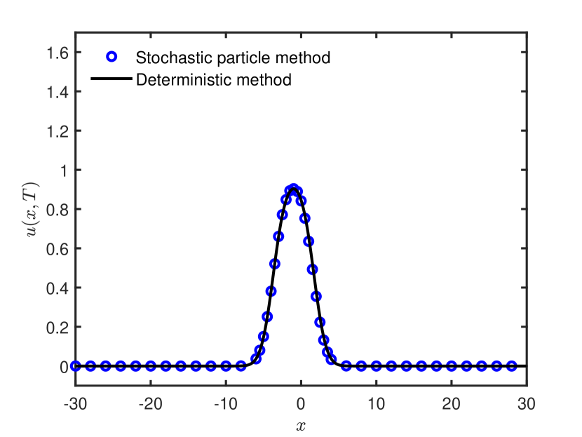
(b) $T=1$, Strategy B.

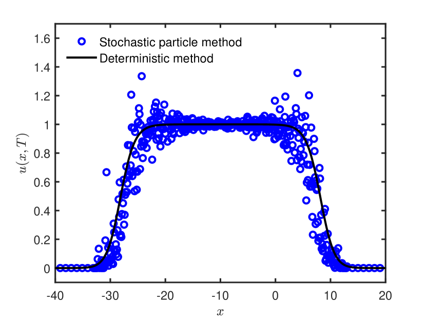
(c) $T=10$, Strategy A.

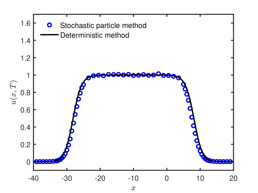
(d) $T=10$, Strategy B.

Figure 3: Strategy A (preliminary strategy) v.s. Strategy B (improved strategy): The relocating technique (see Eq. (19)) adopted by Strategy B may reduce the variance in long-time simulations. Here we set $N=1.6\times 10^{7}$, $\tau=0.1$ and $h=0.1$.

Table 2: Order of SPM: First-order accuracy in both time and space plus half-order accuracy in the sample size. Strategy A and Strategy B are implemented with the final time $T=1$ and $T=10$, respectively.

$N$	$h$	$\tau$	Strategy A, $T=1$		Strategy B, $T=10$
			$\mathcal{E}_{2}[u]$(1)	order	$\mathcal{E}_{2}[u]$(10)	order
$1\times 10^{6}$			0.0574	-	0.0617	-
$4\times 10^{6}$	0.01	0.01	0.0292	$0.49$	0.0316	0.48
$1.6\times 10^{7}$			0.0149	$0.49$	0.0163	0.48
		0.25	0.0355	-	0.0968	-
$1\times 10^{8}$	0.01	$0.2$	0.0288	0.94	0.0792	0.90
		$0.1$	0.0158	$0.88$	0.0422	0.91
	$0.2$		0.0333	-	0.0115	-
$1\times 10^{8}$	$0.15$	0.01	0.0248	0.99	0.0081	1.21
	$0.1$		0.0170	$0.96$	0.0054	1.09

5 Solving the 6-D Allen-Cahn equation

Now we consider the 6-D Allen-Cahn equation

$$\frac{\partial}{\partial t}u(\boldsymbol{x},t)=c\Delta u(\boldsymbol{x},t)+u(\boldsymbol{x},t)-u(\boldsymbol{x},t)^{3}+{r(\boldsymbol{x},t)},\quad\bm{x}\in\mathbb{R}^{6},$$ (35)

which allows the following analytical solution

$$u^{\text{ref}}(\boldsymbol{x},t)=\frac{x_{1}+x_{2}}{\left(\pi(1+4ct)\right)^{d/2}}\left(\exp\left(-\frac{||\boldsymbol{x}-\boldsymbol{p}_{1}||_{2}^{2}}{1+4ct}\right)+2.0\exp\left(-\frac{||\boldsymbol{x}-\boldsymbol{p}_{2}||_{2}^{2}}{1+4ct}\right)\right),$$ (36)

where $\boldsymbol{p}_{1}=\left(2,2,0,\dots,0\right)$, $\boldsymbol{p}_{2}=\left(-1,-1,0,\dots,0\right)$, and $c$ gives the diffusion coefficient which is set to be different values in experiments. The initial data $u_{0}(\bm{x})=u^{\text{ref}}(\boldsymbol{x},0)$ and let $r(\boldsymbol{x},t)$ be the remaining term after substituting the analytical solution Eq. (36) into Eq. (35). We set $\tau=0.1$ in the Lawson-Euler scheme (3) and $h=0.4$ in the piecewise constant reconstruction via VUG adopted by Algorithm 1. In order to visualize high-dimensional solutions, we adopt the following 1-D and 2-D projections

$$P(x_{1},t)=\int_{\mathbb{R}^{d-1}}u(\bm{x},t)\textup{d}x_{2}\dots\textup{d}x_{d},\quad M(x_{1},x_{2},t)=\int_{\mathbbm{R}^{d-2}}u(\bm{x},t)\textup{d}x_{3}\dots\textup{d}x_{d},$$ (37)

and then use the same relative $L^{2}$ errors $\mathcal{E}_{2}[P](t)$ and $\mathcal{E}_{2}[M](t)$ defined in Eq. (34) to measure the accuracy. Table 3, Figures 4 and 5 present the numerical results at the final time $T=2$. All simulations via our C++ implementations run on the High-Performance Computing Platform of Peking University: 2*Intel Xeon E5-2697A-v4 (2.60GHz, 40MB Cache, 9.6GT/s QPI Speed, 16 Cores, 32 Threads) with 256GB Memory $\times$ 16.

Table 3: The 6-D Allen-Cahn equation with diffusion coefficient $c=1$: Total wall time with 8 cores in parallel and the relative $L^{2}$ errors for different sample sizes.

$N$	$\mathcal{E}_{2}[P](2)$	$\mathcal{E}_{2}[M](2)$	Time/h
$1\times 10^{8}$	0.249	0.254	0.27
$2\times 10^{8}$	0.154	0.159	0.53
$4\times 10^{8}$	0.128	0.145	0.96

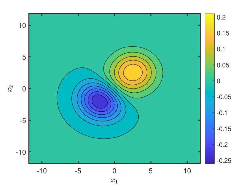
(a) Reference solution.

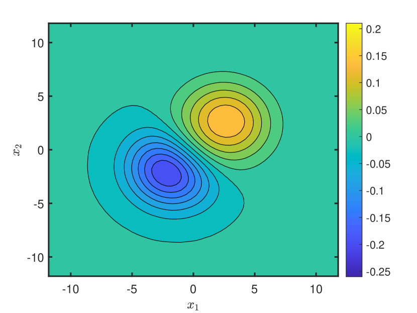
(b) SPM solution with $N=4\times 10^{8}$.

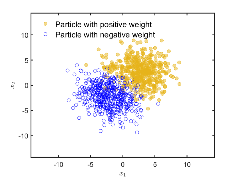
(c) Particle distribution.

Figure 4: The 6-D Allen-Cahn equation with diffusion coefficient $c=1$: Filled contour plots of $M(x_{1},x_{2},2)$ defined in Eq. (37) for (a) the reference solution given in Eq. (36) and (b) the numerical solution produced by SPM with $N=4\times 10^{8}$. The agreement between them is evident. SPM shows a highly adaptive characteristic, and the particles with positive and negative weights adaptively concentrate in the area with positive and negative values of the solution, respectively. This is clearly demonstrated in (c) where we have randomly chosen $10^{3}$ particles from all samples at the final instant $T=2$ and projected their locations onto the $x_{1}x_{2}$-plane.

For the diffusion coefficient $c=1$, SPM takes about an hour using the distributed parallel technology via MPI with 8 cores to evolve the 6-D Allen-Cahn equation (35) until $T=2$ while maintaining the relative $L^{2}$ errors $\mathcal{E}_{2}[P](2)$ and $\mathcal{E}_{2}[M](2)$ less than 15%, see Table 3. Such high efficiency fully benefits from the intrinsic adaptive characteristic of SPM. Figure 4 presents the filled contour plots of $M(x_{1},x_{2},2)$ for the reference solution given in Eq. (36) as well as the SPM solution produced with $N=4\times 10^{8}$ particles. They agree with each other very well and all the particles concentrate in the important areas in an adaptive manner as clearly demonstrated in the last plot of Figure 4, where we have randomly chosen $10^{3}$ particles at the final time and projected their locations into the $x_{1}x_{2}$-plane. In the area where the solution vanishes, there are always few particles. In addition, as displayed in Figure 5, when the diffusion coefficient $c$ increases, the support of the solution expands and thus the memory usage correspondingly increases. In particular, the last plot of Figure 5 shows that the memory consumption increases from $5.4$ GB to $44.1$ GB as $c$ increases from $0.1$ to $1.5$.

(a) SPM solution for $c=0.1$.

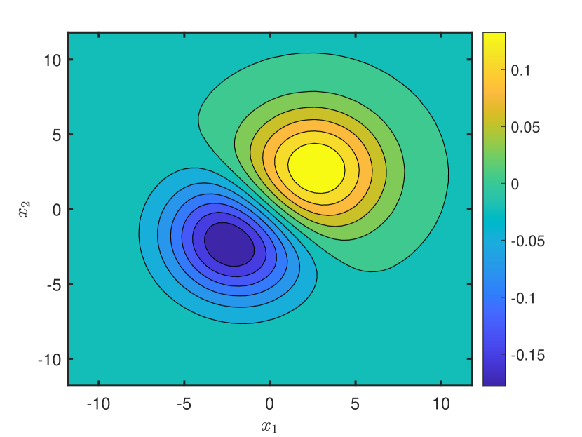
(b) SPM solution for $c=1.5$.

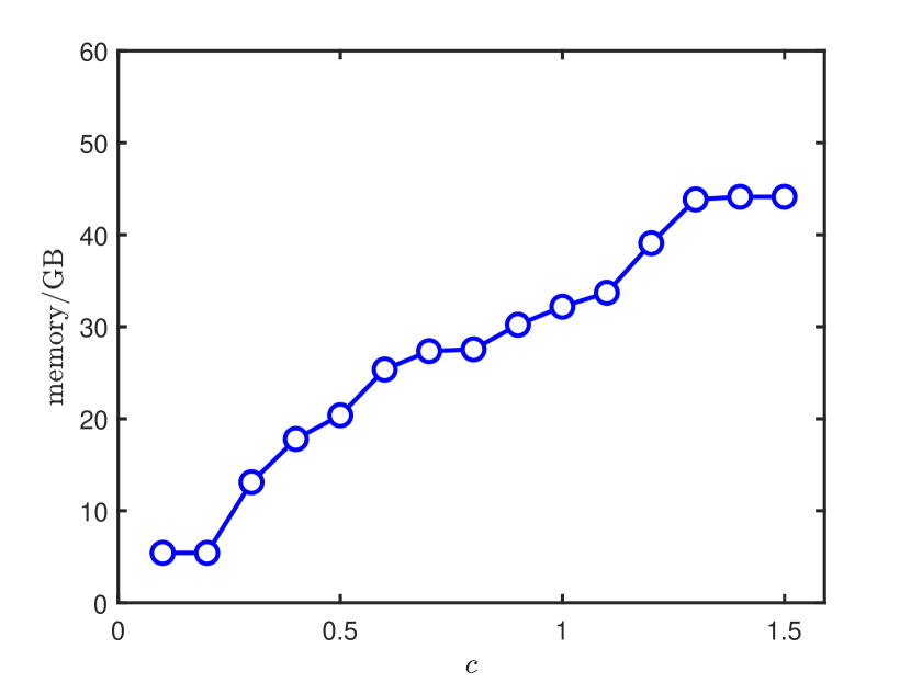
(c) Memory usage against $c$.

Figure 5: The 6-D Allen-Cahn equation: Filled contour plots of $M(x_{1},x_{2},2)$ for (a) $c=0.1$ and (b) $c=1.5$. As the diffusion coefficient $c$ increases, the support of the solution expands and the memory usage correspondingly increases as shown in (c). That is, the memory usage depends on the diffusion coefficient $c$ which may determine the shape of the solution at the same time. Here we set $N=4\times 10^{8}$, too.

6 Solving the 7-D Hamiltonian-Jacobi-Bellman equation

Finally, we apply SPM to integrate the 7-D HJB equation

$$\frac{\partial}{\partial t}u(\boldsymbol{x},t)=c\Delta u(\boldsymbol{x},t)+||\nabla u(\boldsymbol{x},t)||^{2}_{2}+{r(\boldsymbol{x},t)},\quad\bm{x}\in\mathbb{R}^{7},$$ (38)

which admits the following analytical solution

$$u^{\text{ref}}(\boldsymbol{x},t)=\frac{x_{1}^{2}+x_{2}^{2}}{\left(\pi(1+4ct)\right)^{d/2}}\left(2.5\exp\left(-\frac{||\boldsymbol{x}-\boldsymbol{p}_{1}||_{2}^{2}}{1+4ct}\right)-\exp\left(-\frac{||\boldsymbol{x}-\boldsymbol{p}_{2}||_{2}^{2}}{1+4ct}\right)\right),$$ (39)

where $\boldsymbol{p}_{1}=\left(0,0.6,0,\dots,0\right)$, $\boldsymbol{p}_{2}=\left(-1,1,0,\dots,0\right)$ and $c=0.5$. We adopt the same $T,\tau,h$ as in Section 5 and let $\Delta x_{j}=0.4$ in Eq. (24). Figures 6 and 7 plot $M(x_{1},x_{2},2)$ and $P(x_{1},t)$, respectively, defined in Eq. (37) for the numerical solutions produced by SPM with $N=1\times 10^{8},5\times 10^{8}$ and $4\times 10^{9}$ against the reference solution given in Eq. (39). Table 4 shows the corresponding relative $L^{2}$ errors as well as the total wall time. We are able to observe there that, when the number of particles $N$ increases from $1\times 10^{8}$ to $4\times 10^{9}$, the error $\mathcal{E}_{2}[P](2)$ decreases from 30.8% to 6.1% and $\mathcal{E}_{2}[M](2)$ from 34.5% to 10.5%, whereas, in contrast, the computational time with 8 cores shows a sharp increase from about half an hour to $10$ hours and so does the the memory usage.

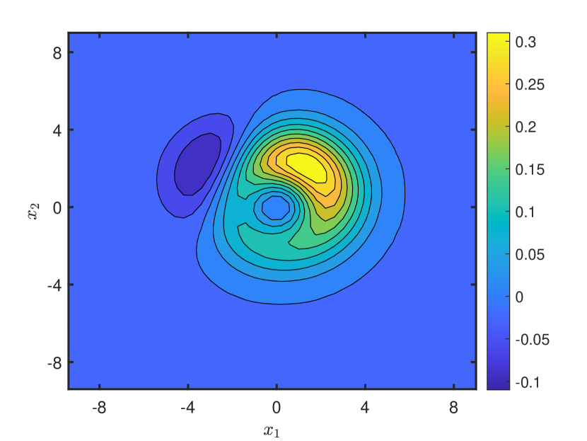
(a) Reference solution.

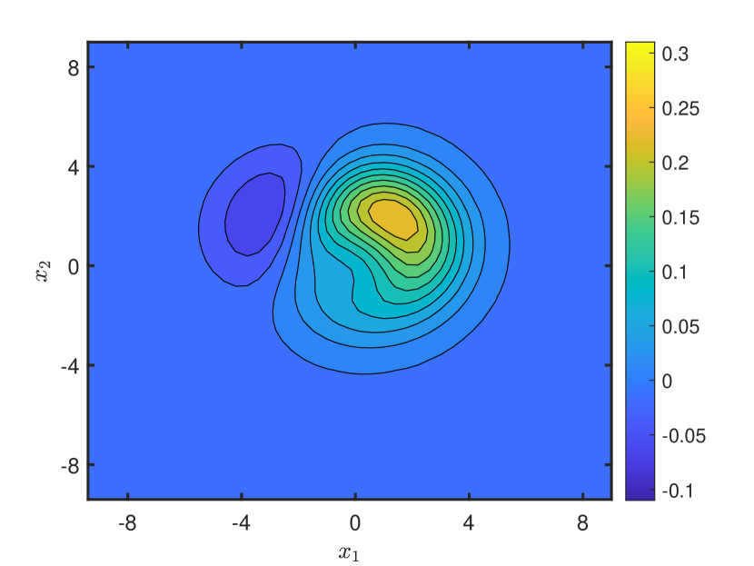
(b) $N=1\times 10^{8}$.

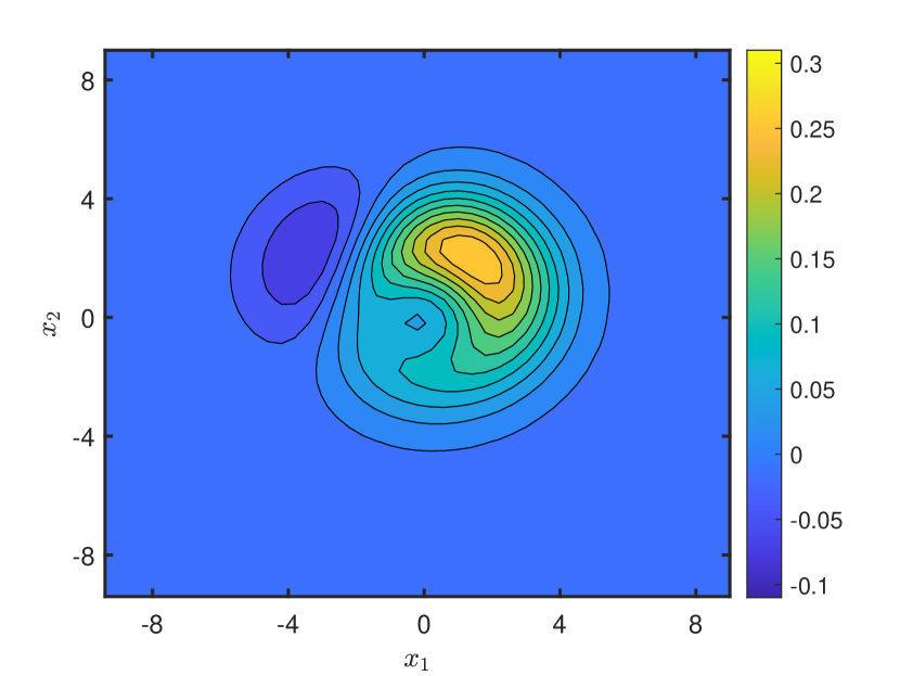
(c) $N=5\times 10^{8}$.

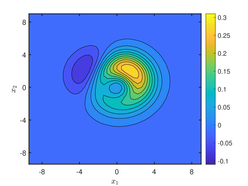
(d) $N=4\times 10^{9}$.

Figure 6: The 7-D HJB equation: Filled contour plots of $M(x_{1},x_{2},2)$ defined in Eq. (37) for (a) the reference solution given in Eq. (39) and the numerical solutions produced by SPM with (b) $N=1\times 10^{8}$, (c) $5\times 10^{8}$ and (d) $4\times 10^{9}$.

Table 4: The 7-D HJB equation: Total wall time with 8 cores in parallel, memory usage and the relative $L^{2}$ errors under different sample sizes.

$N$	$\mathcal{E}_{2}[P](2)$	$\mathcal{E}_{2}[M](2)$	Memory/GB	Time/h
$1\times 10^{8}$	0.308	0.345	17.43	0.39
$5\times 10^{8}$	0.145	0.184	73.58	1.60
$4\times 10^{9}$	0.061	0.105	200.07	9.81

(a) $t=1$.

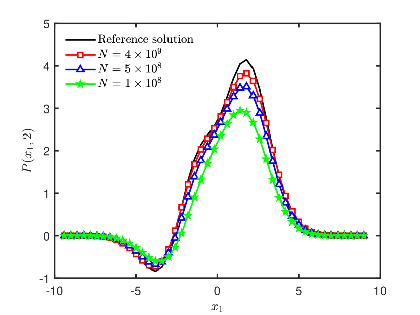
(b) $t=2$.

Figure 7: The 7-D HJB equation: Plots of $P(x_{1},t)$ defined in Eq. (37) at $t=1,2$ for SPM solutions with $N=1\times 10^{8},5\times 10^{8}$ and $4\times 10^{9}$ against the reference solution given in Eq. (39).

7 Conclusion and discussion

This work proposes a stochastic particle method (SPM) to high-dimensional nonlinear PDEs. Starting from the weak formulation of the Lawson-Euler scheme, SPM uses real-valued weighted particles to approximate the high-dimensional solution in the weak sense, and updates the particle locations and weights at each time step. From the perspective of importance sampling, the relocating technique is proposed to make particle locations match the shape of the solution and reduce the stochastic variances. A piecewise constant reconstruction with virtual uniform grid (VUG), which makes full use of the adaptive characteristics of stochastic particles moving with the solution, is adopted for obtaining the values of nonlinear terms. Numerical experiments in solving the 6-D Allen-Cahn equation and the 7-D Hamiltonian-Jacobi-Bellman equation demonstrate the potential of SPM in solving high-dimensional nonlinear PDEs efficiently while maintaining a reasonable accuracy.

Finally, we would like to point out that the proposed SPM can be designed with a probabilistic interpretation starting from its discretization scheme rather than the PDE itself even though the solution of which may not possess a probabilistic interpretation. In this sense, SPM can be regarded as the particle implementation of classical numerical schemes which include finite difference, finite element, spectral methods, etc., and have matured over the last 50 years. Reconstructing the solution values from weighted particles, which is relatively independent, is of high complexity in SPM. In addition to the uniform piecewise constant reconstruction used in this work, the adaptive piecewise constant reconstruction, neural networks and radial basis functions may potentially be combined with stochastic particles, which will be investigated in the future work.

References

- Wigner [1932] E. Wigner, On the quantum corrections for thermodynamic equilibrium, Phys. Rev. 40 (1932) 749–759.
- Black and Scholes [1973] F. Black, M. Scholes, The pricing of options and corporate liabilities, J. Polit. Econ. 81 (1973) 637–654.
- Bellman [1957] R. E. Bellman, Dynamic Programming, Princeton University Press, 1957.
- Cohen and DeVore [2015] A. Cohen, R. DeVore, Approximation of high-dimensional parametric PDEs, Acta Numer. 24 (2015) 1–159.
- Dimarco et al. [2018] G. Dimarco, R. Loubère, J. Narski, T. Rey, An efficient numerical method for solving the Boltzmann equation in multidimensions, J. Comput. Phys. 353 (2018) 46–81.
- Kormann et al. [2019] K. Kormann, K. Reuter, M. Rampp, A massively parallel semi-Lagrangian solver for the six-dimensional Vlasov-Poisson equation, Int. J. High Perform. Comput. Appl. 33 (2019) 924–947.
- Smyth et al. [1998] E. S. Smyth, J. S. Parker, K. T. Taylor, Numerical integration of the time-dependent Schrödinger equation for laser-driven Helium, Commun. Comput. Phys. 114 (1998) 1–14.
- Xiong et al. [2023] Y. Xiong, Y. Zhang, S. Shao, A characteristic-spectral-mixed scheme for six-dimensional Wigner-Coulomb dynamics, To appear in SIAM J. Sci. Comput. (2023).
- Jiang et al. [2017] K. Jiang, P. Zhang, A. Shi, Stability of icosahedral quasicrystals in a simple model with two-length scales, J. Phys.: Condens. Matter 29 (2017) 124003.
- Li et al. [2013] M. Li, W. Chen, C. S. Chen, The localized RBFs collocation methods for solving high dimensional PDEs, Eng. Anal. Bound. Elem. 37 (2013) 1300–1304.
- Giles [2008] M. B. Giles, Multilevel Monte Carlo path simulation, Oper. Res. 56 (2008) 607–617.
- Wang and Sloan [2005] X. Wang, I. H. Sloan, Why are high-dimensional finance problems often of low effective dimension?, SIAM J. Sci. Comput. 27 (2005) 159–183.
- Bayer et al. [2023] C. Bayer, M. Eigel, L. Sallandt, P. Trunschke, Pricing high-dimensional Bermudan options with hierarchical tensor formats, SIAM J. Financ. Math. 14 (2023) 383–406.
- E et al. [2020] W. E, C. Ma, L. Wu, Machine learning from a continuous viewpoint, Sci. China Math. 63 (2020) 2233–2266.
- Han et al. [2018] J. Han, A. Jentzen, W. E, Solving high-dimensional partial differential equations using deep learning, P. Natl. Acad. Sci. USA 115 (2018) 8505–8510.
- Raissi et al. [2019] M. Raissi, P. Perdikaris, G. E. Karniadakis, Physics-informed neural networks: A deep learning framework for solving forward and inverse problems involving nonlinear partial differential equations, J. Comput. Phys. 378 (2019) 1547–1579.
- Huré et al. [2020] C. Huré, H. Pham, X. Warin, Deep backward schemes for high-dimensional nonlinear PDEs, Math. Comp. 89 (2020) 1547–1579.
- Gao and Wang [2023] W. Gao, C. Wang, Active learning based sampling for high-dimensional nonlinear partial differential equations, J. Comput. Phys. 475 (2023) 111848.
- Courant et al. [1928] R. Courant, K. Friedrichs, H. Lewy, Über die partiellen differenzengleichungen der mathematischen physik, Math. Ann. 100 (1928) 32–74.
- Pierre et al. [2019] H. L. Pierre, O. Nadia, X. Tan, N. Touzi, X. Warin, Branching diffusion representation of semilinear PDEs and Monte Carlo approximation, Ann. Inst. H. Poincaré Probab. Statist. 55 (2019) 184–210.
- E et al. [2019] W. E, H. Martin, J. Arnulf, K. Thomas, On multilevel picard numerical approximations for high-dimensional nonlinear parabolic partial differential equations and high-dimensional nonlinear backward stochastic differential equations, J. Sci. Comput. 79 (2019) 1534–1571.
- Mainini [2012] E. Mainini, A description of transport cost for signed measures, J. Math. Sci. 181 (2012) 837–855.
- Ambrosio et al. [2011] L. Ambrosio, E. Mainini, S. Serfaty, Gradient flow of the Chapman-Rubinstein-Schatzman model for signed vortices, Ann. Inst. H. Poincaré Anal. Non linéaire 28 (2011) 217–246.
- Piccoli et al. [2019] B. Piccoli, F. Rossi, M. Tournus, A Wasserstein norm for signed measures, with application to nonlocal transport equation with source term, arXiv preprint arXiv:1910.05105 (2019).
- Lawson [1967] J. D. Lawson, Generalized Runge-Kutta processes for stable systems with large Lipschitz constants, SIAM J. Numer. Anal. 4 (1967) 372–380.
- Li et al. [2016] D. Li, K. Yang, W. Wong, Density estimation via discrepancy based adaptive sequential partition, Adv. Neural. Inf. Process. Syst. (2016) 1091–1099.
- Hochbruck and Ostermann [2010] M. Hochbruck, A. Ostermann, Exponential integrators, Acta Numer. 19 (2010) 209–286.
- Dimov [2008] I. T. Dimov, Monte Carlo Methods for Applied Scientists, World Scientific, 2008.
- Shao and Xiong [2020] S. Shao, Y. Xiong, Branching random walk solutions to the Wigner equation, SIAM J. Numer. Anal. 58(5) (2020) 2589–2608.
- Raviart [1983] P. A. Raviart, An analysis of particle methods, in: Numerical Methods in Fluid Dynamics. Vol. 1127 of Lecture Notes in Mathematics., Springer, 1983, pp. 243–324.
- Yan and Caflisch [2015] B. Yan, R. E. Caflisch, A Monte Carlo method with negative particles for Coulomb collisions, J. Comput. Phys. 298 (2015) 711–740.
- Wu et al. [2017] K. Wu, Y. Shin, D. Xiu, A randomized tensor quadrature method for high dimensional polynomial approximation, SIAM J. Sci. Comput. 39 (2017) A1811–A1833.
- Wu and Xiu [2018] K. Wu, D. Xiu, Sequential function approximation on arbitrarily distributed point sets, J. Comput. Phys. 354 (2018) 370–386.
- Beylkin et al. [1998] G. Beylkin, J. M. Keiser, L. Vozovoi, A new class of time discretization schemes for the solution of nonlinear PDEs, J. Comput. Phys. 147 (1998) 362–387.
- Hansen et al. [2012] E. Hansen, F. Kramer, A. Ostermann, A second-order positivity preserving scheme for semilinear parabolic problems, Appl. Numer. Math. 62 (2012) 1428–1435.
- Crouseilles et al. [2020] N. Crouseilles, L. Einkemmer, J. Massot, Exponential methods for solving hyperbolic problems with application to collisionless kinetic equations, J. Comput. Phys. 420 (2020) 109688.
- Gnewuch et al. [2012] M. Gnewuch, M. Wahlström, C. Winzen, A new randomized algorithm to approximate the star discrepancy based on threshold accepting, SIAM J. Numer. Anal. 50(2) (2012) 781–807.
- Xiong and Shao [2019] Y. Xiong, S. Shao, The Wigner branching random walk: Efficient implementation and performance evaluation, Commun. Comput. Phys. 25 (2019) 871–910.
- Silverman [2018] B. W. Silverman, Density Estimation for Statistics and Data Analysis, Routledge, 2018.