Nonuniform Bose-Einstein condensate. I.
An improvement of the Gross-Pitaevskii method

A nonuniform condensate is usually described by the Gross-Pitaevskii (GP) equation, which is derived with the help of the c-number ansatz $\hat{\Psi}(\mathbf{r},t)=\Psi(\mathbf{r},t)$. Proceeding from a more accurate operator ansatz $\hat{\Psi}(\mathbf{r},t)=\hat{a}_{0}\Psi(\mathbf{r},t)\sqrt{N}$, we find the equation $i\hbar\frac{\partial\Psi(\mathbf{r},t)}{\partial t}=-\frac{\hbar^{2}}{2m}\frac{\partial^{2}\Psi(\mathbf{r},t)}{\partial\mathbf{r}^{2}}+\left(1-\frac{1}{N}\right)2c\Psi(\mathbf{r},t)|\Psi(\mathbf{r},t)|^{2}$ (the GP_N equation). It differs from the GP equation by the factor $\left(1-1/N\right)$, where $N$ is the number of Bose particles. We compare the accuracy of the GP and GP_N equations by analyzing the ground state of a one-dimensional system of point bosons with repulsive interaction ($c>0$) and zero boundary conditions. Both equations are solved numerically, and the system energy $E$ and the particle density profile $\rho(x)$ are determined for various values of $N$, the mean particle density $\bar{\rho}$, and the coupling constant $\gamma=c/\bar{\rho}$. The solutions are compared with the exact ones obtained by the Bethe ansatz. The results show that in the weak coupling limit ($N^{-2}\ll\gamma\lesssim 0.1$), the GP and GP_N equations describe the system equally well if $N\gtrsim 100$. For few-boson systems ($N\lesssim 10$) with $\gamma\lesssim N^{-2}$ the solutions of the GP_N equation are in excellent agreement with the exact ones. That is, the multiplier $\left(1-1/N\right)$ allows one to describe few-boson systems with high accuracy. This means that it is reasonable to extend the notion of Bose-Einstein condensation to few-particle systems.

1 Introduction

The simplest analytical method for describing a system of $N$ spinless interacting bosons is based on the solution of the nonlinear Schrödinger equation

$$i\hbar\frac{\partial\Psi(\mathbf{r},t)}{\partial t}=-\frac{\hbar^{2}}{2m}\frac{\partial^{2}\Psi(\mathbf{r},t)}{\partial\mathbf{r}^{2}}+\Psi(\mathbf{r},t)\int\limits_{V}d\mathbf{r}^{\prime}U(|\mathbf{r}-\mathbf{r}^{\prime}|)|\Psi(\mathbf{r}^{\prime},t)|^{2},$$ (1)

where $\Psi$ is the wave function of condensate, $V$ is the system volume. This equation was first obtained by E. Gross in 1958 [1, 2]. Gross realised that N. Bogoliubov’s approach [3] could be applied to describe a nonuniform condensate if we set $\hat{\Psi}(\mathbf{r},t)=\Psi(\mathbf{r},t)$. In this case, the Heisenberg equation becomes Eq. (1) for $\Psi(\mathbf{r},t)$. A few years later, Eq. (1) was written by L. Pitaevskii [4] and E. Gross [5] for the point potential $U(|\mathbf{r}_{j}-\mathbf{r}_{l}|)=2c\delta(\mathbf{r}_{j}-\mathbf{r}_{l})$,

$$i\hbar\frac{\partial\Psi(\mathbf{r},t)}{\partial t}=-\frac{\hbar^{2}}{2m}\frac{\partial^{2}\Psi(\mathbf{r},t)}{\partial\mathbf{r}^{2}}+2c\Psi(\mathbf{r},t)|\Psi(\mathbf{r},t)|^{2}.$$ (2)

Since real-world atoms have a non-zero size, it is more accurate to describe them by Eq. (1). However, if the characteristic dimensions of inhomogeneities in the system are much larger than the atomic size, the Gross-Pitaevskii (GP) equation (2) may be used instead of Eq. (1). The GP equation is simpler than the Gross equation (1) and is basic for describing the dilute Bose gas in a trap. A huge number of experimental and theoretical works published during the last 25 years were devoted to the study of gases in the trap [6, 7, 8, 9]. The Nobel Prize was awarded for the experimental production of Bose condensate [10, 11].

It is generally accepted that Eqs. (1) and (2) give a semiclassical description of the system and are only applicable to systems with a large number of particles, $N$. Several arguments have been made in favour of the latter [9, 12, 13, 14]. The main one is that the Bogoliubov method works namely at $N\gg 1$.

It is often asserted that Eqs. (1) and (2) can also be derived from the condensate approximation for the total $N$-particle wave function of the system

$$\Psi_{N}(\mathbf{r}_{1},\ldots,\mathbf{r}_{N},t)=\prod\limits_{j=1}^{N}\psi(\mathbf{r}_{j},t).$$ (3)

However, this is not quite so. By integrating the $N$-particle Schrödinger equation [15] (see also section 2 below) and by using a variational approach [16] it was shown that ansatz (3) gives rise to the equation

$$i\hbar\frac{\partial\Psi(\mathbf{r},t)}{\partial t}=-\frac{\hbar^{2}}{2m}\frac{\partial^{2}\Psi(\mathbf{r},t)}{\partial\mathbf{r}^{2}}+\left(1-\frac{1}{N}\right)\Psi(\mathbf{r},t)\int\limits_{V}d\mathbf{r}^{\prime}U(|\mathbf{r}-\mathbf{r}^{\prime}|)|\Psi(\mathbf{r}^{\prime},t)|^{2}.$$ (4)

For the potential $U(|\mathbf{r}_{j}-\mathbf{r}_{l}|)=2c\delta(\mathbf{r}_{j}-\mathbf{r}_{l})$ it transforms into

$$i\hbar\frac{\partial\Psi(\mathbf{r},t)}{\partial t}=-\frac{\hbar^{2}}{2m}\frac{\partial^{2}\Psi(\mathbf{r},t)}{\partial\mathbf{r}^{2}}+\left(1-\frac{1}{N}\right)2c\Psi(\mathbf{r},t)|\Psi(\mathbf{r},t)|^{2}.$$ (5)

It will be seen in section 2 below that if the more accurate operator ansatz

$$\hat{\Psi}(\mathbf{r},t)=\hat{a}_{0}\Psi(\mathbf{r},t)/\sqrt{N}$$ (6)

is used instead of the c-number ansatz $\hat{\Psi}(\mathbf{r},t)=\Psi(\mathbf{r},t)$, we also get Eqs. (4) and (5).

Equations (2) and (5) will be called the GP and GP_N equations, respectively. The GP_N equation differs from the GP one by the factor $\left(1-1/N\right)$. This equation was obtained using ansätze (3) and (6), which are valid for any $N\geq 2$ (in contrast to the ansatz $\hat{\Psi}(\mathbf{r},t)\approx\Psi(\mathbf{r},t)$, which is only applicable for $N\gg 1$). This indicates that the GP_N equation must be able to describe a Bose system even for small $N$.

The accuracy of the GP_N equation has already been investigated for a Bose gas under spherically symmetric harmonic confinement by comparing solutions of the GP_N equation with Monte Carlo numerical solutions for $N=2$–$50$ [17] and with analytical solutions of the linear Schrödinger equation for $N=2$ [8]. Such an analysis showed that for $0\leq(N-1)a/a_{h0}\ \lower-1.2pt\vbox{\hbox{\hbox to0.0pt{$<$\hss}\lower 5.0pt\vbox{\hbox{$\sim$}}}}\ 0.1$ (where $a$ is the s-wave scattering length, and $a_{h0}=(\hbar/m\omega_{h0})^{1/2}$), the GP_N equation describes the system with very good accuracy. However, the comparison of the accuracy of the GP_N and GP equations has not yet been carried out.

In this and the next paper [18] we study in detail a one-dimensional (1D) Bose gas in the absence of a trap and compare the solutions of stationary GP and GP_N equations for different $N\geq 2$ with the exact Bethe-ansatz solutions. In this paper, an equation for a nonuniform condensate is derived (section 2) and its solutions for the ground state of the condensate are analyzed (sections 3–5). In the next article [18], the excited states of the condensate are considered.

Note that we became aware of papers [15, 16, 17, 8] after this article was submitted to arXiv. Moreover, after this article and [18] had already been written, we learned that analogous solutions of the GP equation have been found analytically by L. Carr, C. Clark, and W. Reinhardt [19]. The solutions obtained in [19] are expressed in terms of the Jacobi elliptic functions. In this paper, we obtain solutions using a different (numerical) method. Our solutions are consistent with those of work [19], although a detailed one-to-one comparison was not performed.

Note also that in the 1D case the term quasi-condensate is usually used instead of condensate [7, 20, 21]. For brevity, we will omit the prefix “quasi” and write “condensate”, even for small $N$.

2 Derivation of equation for nonuniform condensate

2.1 Wave-function approach

Consider a system of $N$ interacting spinless bosons ($N\geq 2$). The Schrödinger equation reads

$$i\hbar\frac{\partial\Psi_{N}}{\partial t}=-\frac{\hbar^{2}}{2m}\sum\limits_{j=1}^{N}\frac{\partial^{2}}{\partial\mathbf{r}_{j}^{2}}\Psi_{N}+\frac{1}{2}\mathop{\sum^{N}_{j,p=1}}\limits_{(j\neq p)}U(|\mathbf{r}_{p}-\mathbf{r}_{j}|)\Psi_{N}.$$ (7)

Let the wave function $\Psi_{N}(\mathbf{r}_{1},\ldots,\mathbf{r}_{N},t)$ of the system have the condensate form (3) with the normalization $|\psi(\mathbf{r},t)|^{2}=1$. Substituting (3) into (7), we obtain

$$i\hbar\sum\limits_{j=1}^{N}\mathop{\prod^{N}_{l=1}}\limits_{(l\neq j)}\psi(\mathbf{r}_{l},t)\cdot\frac{\partial\psi(\mathbf{r}_{j},t)}{\partial t}=$$ (8)

$$= -\frac{\hbar^{2}}{2m}\sum\limits_{j=1}^{N}\mathop{\prod^{N}_{l=1}}\limits_{(l\neq j)}\psi(\mathbf{r}_{l},t)\cdot\frac{\partial^{2}\psi(\mathbf{r}_{j},t)}{\partial\mathbf{r}_{j}^{2}}+\frac{1}{2}\mathop{\sum^{N}_{j,p=1}}\limits_{(p\neq j)}U(|\mathbf{r}_{p}-\mathbf{r}_{j}|)\prod\limits_{l=1}^{N}\psi(\mathbf{r}_{l},t).$$

Multiplying this equation by $\prod_{l=2}^{N}\psi^{\ast}(\mathbf{r}_{l},t)$ and integrating the result over $\mathbf{r}_{2},\ldots,\mathbf{r}_{N}$, we get

$$i\hbar\frac{\partial\psi(\mathbf{r}_{1},t)}{\partial t}-a(t)\psi(\mathbf{r}_{1},t)=-\frac{\hbar^{2}}{2m}\frac{\partial^{2}\psi(\mathbf{r}_{1},t)}{\partial\mathbf{r}_{1}^{2}}$$

$$+(N-1)\psi(\mathbf{r}_{1},t)\int\limits_{V}d\mathbf{r}_{2}U(|\mathbf{r}_{1}-\mathbf{r}_{2}|)|\psi(\mathbf{r}_{2},t)|^{2},$$ (9)

where

$$a(t) = (N-1)\int\limits_{V}d\mathbf{r}_{2}\psi^{\ast}(\mathbf{r}_{2},t)\left\{-\frac{\hbar^{2}}{2m}\frac{\partial^{2}\psi(\mathbf{r}_{2},t)}{\partial\mathbf{r}_{2}^{2}}-i\hbar\frac{\partial\psi(\mathbf{r}_{2},t)}{\partial t}\right\}$$ (10)

$$+ \frac{(N-1)(N-2)}{2}\int\limits_{V}d\mathbf{r}_{2}d\mathbf{r}_{3}U(|\mathbf{r}_{2}-\mathbf{r}_{3}|)|\psi(\mathbf{r}_{2},t)|^{2}|\psi(\mathbf{r}_{3},t)|^{2}.$$

The derivatives in the right-hand side of (10) can be expressed using Eq. (9), from whence

$$a(t)=-\frac{(N-1)}{2}\int\limits_{V}d\mathbf{r}_{2}d\mathbf{r}_{3}U(|\mathbf{r}_{2}-\mathbf{r}_{3}|)|\psi(\mathbf{r}_{2},t)|^{2}|\psi(\mathbf{r}_{3},t)|^{2}.$$ (11)

Let us set $\psi(\mathbf{r}_{1},t)=e^{i\kappa(t)/\hbar}\tilde{\psi}(\mathbf{r}_{1},t)$, where $\kappa(t)=-\int_{-\infty}^{t}d\tau a(\tau)$ [15]. Then (9) is reduced to

$$i\hbar\frac{\partial\tilde{\psi}(\mathbf{r}_{1},t)}{\partial t}=-\frac{\hbar^{2}}{2m}\frac{\partial^{2}\tilde{\psi}(\mathbf{r}_{1},t)}{\partial\mathbf{r}_{1}^{2}}+(N-1)\tilde{\psi}(\mathbf{r}_{1},t)\int\limits_{V}d\mathbf{r}_{2}U(|\mathbf{r}_{1}-\mathbf{r}_{2}|)|\tilde{\psi}(\mathbf{r}_{2},t)|^{2}.$$ (12)

Making the substitution $\psi(\mathbf{r},t)=\Psi(\mathbf{r},t)/\sqrt{N}$, we obtain the final equation

$$i\hbar\frac{\partial\Psi(\mathbf{r},t)}{\partial t}=-\frac{\hbar^{2}}{2m}\frac{\partial^{2}\Psi(\mathbf{r},t)}{\partial\mathbf{r}^{2}}+\left(1-\frac{1}{N}\right)\Psi(\mathbf{r},t)\int\limits_{V}d\mathbf{r}^{\prime}U(|\mathbf{r}-\mathbf{r}^{\prime}|)|\Psi(\mathbf{r}^{\prime},t)|^{2},$$ (13)

with the normalization $\int_{V}d\mathbf{r}|\Psi(\mathbf{r},t)|^{2}=N$. For the point potential $U(|\mathbf{r}_{j}-\mathbf{r}_{l}|)=2c\delta(\mathbf{r}_{j}-\mathbf{r}_{l})$, this equation reads

$$i\hbar\frac{\partial\Psi(\mathbf{r},t)}{\partial t}=-\frac{\hbar^{2}}{2m}\frac{\partial^{2}\Psi(\mathbf{r},t)}{\partial\mathbf{r}^{2}}+\left(1-\frac{1}{N}\right)2c\Psi(\mathbf{r},t)|\Psi(\mathbf{r},t)|^{2}.$$ (14)

It has come to our attention that a similar analysis was previously carried out by B. Esry [15].

It is worth noting that the condensate ansatz (3) does not satisfy the Schrödinger equation (7) for any non-zero potential, even if Eqs. (9) and (11) are satisfied. Therefore, ansatz (3) always gives only an approximate description of the system. For the description to be exact, two-particle and all higher-order correlations in $\Psi_{N}(\mathbf{r}_{1},\ldots,\mathbf{r}_{N},t)$ must be taken into account [6, 22, 23, 24, 25].

2.2 Operator method

T. Wu in work [26] proposed a method for describing a system of point bosons, which is based on the ansatz $\hat{\Psi}(\mathbf{r},t)=\hat{a}_{0}\psi(\mathbf{r},t)+\hat{\vartheta}(\mathbf{r},t)$ with $\hat{\vartheta}(\mathbf{r},t)\ll\hat{a}_{0}\psi(\mathbf{r},t)$. The analysis [26] resulted in Eqs. (9), (11) with $U(|\mathbf{r}_{j}-\mathbf{r}_{l}|)\rightarrow 2c\delta(\mathbf{r}_{j}-\mathbf{r}_{l})$ and $N-1\rightarrow N$. We are unable to reproduce Wu’s analysis, so we will make an independent calculation in the simpler case $\hat{\Psi}(\mathbf{r},t)=\hat{a}_{0}\psi(\mathbf{r},t)$ with the normalization $\int_{V}d\mathbf{r}|\psi(\mathbf{r},t)|^{2}=1$. Thus, we assume that all $N$ atoms at any time are in the condensate $\psi(\mathbf{r},t)$, but we do not change to the c-number. Substituting $\hat{\Psi}(\mathbf{r},t)=\hat{a}_{0}\psi(\mathbf{r},t)$ into the Heisenberg equation

$$i\hbar\frac{\partial\hat{\Psi}(\mathbf{r},t)}{\partial t}=-\frac{\hbar^{2}}{2m}\frac{\partial^{2}\hat{\Psi}(\mathbf{r},t)}{\partial\mathbf{r}^{2}}+\int\limits_{V}d\mathbf{r}^{\prime}U(|\mathbf{r}-\mathbf{r}^{\prime}|)\hat{\Psi}^{+}(\mathbf{r}^{\prime},t)\hat{\Psi}(\mathbf{r}^{\prime},t)\cdot\hat{\Psi}(\mathbf{r},t),$$ (15)

we obtain

$$\hat{G}=0,$$ (16)

where

$$\hat{G} = -\hat{a}_{0}i\hbar\frac{\partial\psi(\mathbf{r},t)}{\partial t}-\psi(\mathbf{r},t)i\hbar\frac{\partial\hat{a}_{0}}{\partial t}-\hat{a}_{0}\frac{\hbar^{2}}{2m}\frac{\partial^{2}\psi(\mathbf{r},t)}{\partial\mathbf{r}^{2}}+$$ (17)

$$+\hat{a}_{0}^{+}\hat{a}_{0}^{2}\psi(\mathbf{r},t)\int\limits_{V}d\mathbf{r}^{\prime}U(|\mathbf{r}-\mathbf{r}^{\prime}|)|\psi(\mathbf{r}^{\prime},t)|^{2}.$$

Consider an $N$-particle state $|N_{0},N_{1},N_{2},\ldots,N_{\infty}\rangle$, where $N_{0}=N$ particles are in the one-particle state $\psi_{0}(\mathbf{r},t)\equiv\psi(\mathbf{r},t)$, whereas the other one-particle states $\psi_{j}$ from the expansion $\hat{\Psi}(\mathbf{r},t)=\sum_{j=0,1,\ldots,\infty}\hat{a}_{j}(t)\psi_{j}(\mathbf{r},t)$ are non-occupied, $N_{j\geq 1}=0$. Denote $|N,0,\ldots,0\rangle\equiv|N\rangle$. The expression

$$\hat{G}|N\rangle=0$$ (18)

sets the equation for the condensate $\psi(\mathbf{r},t)$ for the system in the $|N\rangle$ state. To find $\hat{G}|N\rangle$, we have to calculate $\partial\hat{a}_{0}/\partial t$. If $\hat{\Psi}(\mathbf{r},t)=\hat{a}_{0}\psi(\mathbf{r},t)$, the system Hamiltonian takes the form

$$\hat{H} = -\frac{\hbar^{2}}{2m}\int d\mathbf{r}\hat{\Psi}^{+}(\mathbf{r},t)\frac{\partial^{2}\hat{\Psi}(\mathbf{r},t)}{\partial\mathbf{r}^{2}}+\frac{1}{2}\int d\mathbf{r}d\mathbf{r}^{\prime}U(|\mathbf{r}-\mathbf{r}^{\prime}|)\hat{\Psi}^{+}(\mathbf{r},t)\hat{\Psi}^{+}(\mathbf{r}^{\prime},t)\hat{\Psi}(\mathbf{r}^{\prime},t)\hat{\Psi}(\mathbf{r},t)$$ (19)

$$= E_{k}\hat{a}_{0}^{+}(t)\hat{a}_{0}(t)+E_{p}[\hat{a}_{0}^{+}(t)]^{2}\hat{a}_{0}^{2}(t)=(E_{k}-E_{p})\hat{N}_{0}(t)+E_{p}\hat{N}_{0}^{2}(t),$$

where $\hat{N}_{0}(t)=\hat{a}_{0}^{+}(t)\hat{a}_{0}(t)$,

$$E_{k}=-\frac{\hbar^{2}}{2m}\int d\mathbf{r}\psi^{\ast}(\mathbf{r},t)\frac{\partial^{2}\psi(\mathbf{r},t)}{\partial\mathbf{r}^{2}},$$ (20)

$$E_{p}=\frac{1}{2}\int d\mathbf{r}d\mathbf{r}^{\prime}U(|\mathbf{r}-\mathbf{r}^{\prime}|)|\psi(\mathbf{r},t)|^{2}|\psi(\mathbf{r}^{\prime},t)|^{2}.$$ (21)

Such a Hamiltonian does not contain terms that could transfer atoms from the condensate to other states $\psi_{j\geq 1}(\mathbf{r},t)$. Therefore it is natural to expect that $\frac{\partial\hat{a}_{0}}{\partial t}=0$.

Let us show that really $\frac{\partial\hat{a}_{0}}{\partial t}=0$. The derivative $\frac{\partial\hat{a}_{0}}{\partial t}$ cannot be found from the Heisenberg equation $i\hbar\frac{\partial\hat{a}_{0}}{\partial t}=[\hat{a}_{0},\hat{H}]$. Indeed, from the equations $i\hbar\frac{\partial\hat{a}_{j}}{\partial t}=[\hat{a}_{j},\hat{H}]$ ($j=0,1,\ldots,\infty$), $\hat{\Psi}(\mathbf{r},t)=\sum_{j=0,1,\ldots,\infty}\hat{a}_{j}(t)\psi_{j}(\mathbf{r},t)$, and $i\hbar\frac{\partial\hat{\Psi}}{\partial t}=[\hat{\Psi},\hat{H}]$, it follows that $\sum_{j=0,1,\ldots,\infty}\hat{a}_{j}(t)\frac{\partial\psi_{j}(\mathbf{r},t)}{\partial t}=0$, i.e. $\sum_{j=0,1,\ldots,\infty}\hat{a}_{j}^{+}(t)\frac{\partial\psi_{j}^{\ast}(\mathbf{r},t)}{\partial t}=0$. The last two equations must hold for any state $|N_{0},N_{1},\ldots,N_{\infty}\rangle$. This means that $\frac{\partial\psi_{j}^{\ast}(\mathbf{r},t)}{\partial t}=0$ and $\frac{\partial\psi_{j}(\mathbf{r},t)}{\partial t}=0$ for all $j=0,1,\ldots,\infty$, which contradicts our scheme.

Similarly to the analysis in [26], let us determine $\frac{\partial\hat{a}_{0}}{\partial t}$ from the time evolution of the wave function in the Schrödinger representation: $\Psi(\mathbf{r},t)=e^{-i\hat{H}t/\hbar}\Psi(\mathbf{r})$ [27]. Then

$$\Psi(\mathbf{r},t+\delta t)=e^{-i\hat{H}\delta t/\hbar}\Psi(\mathbf{r},t).$$ (22)

In the second quantization formalism, the state $|N,0,0,\ldots,0\rangle$ is [27]

$$\Psi(t)=(N!)^{-1/2}[\hat{a}_{0}^{+}(t)]^{N}|0\rangle,$$ (23)

where $|0\rangle\equiv|0,0,0,\ldots,0\rangle$ is the vacuum state:

$$\hat{a}_{j}|0\rangle=0,\quad j=0,1,2,\ldots,\infty.$$ (24)

Then

$$\Psi(t+\delta t) \equiv (N!)^{-1/2}[\hat{a}_{0}^{+}(t+\delta t)]^{N}|0\rangle=e^{-i\hat{H}\delta t/\hbar}\Psi(t)=(N!)^{-1/2}e^{-i\hat{H}\delta t/\hbar}[\hat{a}_{0}^{+}(t)]^{N}|0\rangle$$ (25)

$$= (N!)^{-1/2}\left(1-i\hat{H}\delta t/\hbar+\frac{1}{2!}(-i\hat{H}\delta t/\hbar)^{2}+\ldots\right)[\hat{a}_{0}^{+}(t)]^{N}|0\rangle.$$

Note that the energy and the total number of particles are integrals of motion; therefore, $\hat{H}$ and $\hat{N}$ do not depend on time. Using the relations

$$\hat{a}_{0}(t)\hat{a}_{0}^{+}(t)=\hat{a}_{0}^{+}(t)\hat{a}_{0}(t)+1,$$ (26)

$$\hat{N}_{0}(t)[\hat{a}_{0}^{+}(t)]^{N}=[\hat{a}_{0}^{+}(t)]^{N}(\hat{N}_{0}(t)+N),$$ (27)

$$\hat{N}_{0}(t)^{2}[\hat{a}_{0}^{+}(t)]^{N}=[\hat{a}_{0}^{+}(t)]^{N}(\hat{N}_{0}(t)+N)^{2},$$ (28)

and formula (19), we obtain

$$(-\hat{H}\delta t/\hbar)^{p}[\hat{a}_{0}^{+}(t)]^{N}=[\hat{a}_{0}^{+}(t)]^{N}\hat{f}^{p},$$ (29)

$$\hat{f}=(-\delta t/\hbar)\left[(E_{k}-E_{p})(\hat{N}_{0}(t)+N)+E_{p}(\hat{N}_{0}(t)+N)^{2}\right],$$ (30)

$$(N!)^{-1/2}[\hat{a}_{0}^{+}(t+\delta t)]^{N}|0\rangle=(N!)^{-1/2}[\hat{a}_{0}^{+}(t)]^{N}e^{i\hat{f}}|0\rangle$$ (31)

$$= (N!)^{-1/2}[\hat{a}_{0}^{+}(t)]^{N}\left(1+i\hat{f}+\frac{1}{2!}(i\hat{f})^{2}+\ldots\right)|0\rangle.$$

Since

$$i\hat{f}|0\rangle=(-i\delta t/\hbar)\left[(E_{k}-E_{p})N+E_{p}N^{2}\right]|0\rangle\equiv ig\delta t|0\rangle,$$ (32)

we have that for an arbitrary $\delta t\geq 0$,

$$(N!)^{-1/2}[\hat{a}_{0}^{+}(t+\delta t)]^{N}|0\rangle=e^{ig\delta t}(N!)^{-1/2}[\hat{a}_{0}^{+}(t)]^{N}|0\rangle.$$ (33)

To find the correct normalization, we must make the substitution $e^{ig\delta t}\rightarrow 1$. Eventually,

$$(N!)^{-1/2}[\hat{a}_{0}^{+}(t+\delta t)]^{N}|0\rangle=(N!)^{-1/2}[\hat{a}_{0}^{+}(t)]^{N}|0\rangle,$$ (34)

$$\hat{a}_{0}^{+}(t+\delta t)=\hat{a}_{0}^{+}(t),\quad\partial\hat{a}_{0}^{+}/\partial t=0\quad\Rightarrow\ \partial\hat{a}_{0}/\partial t=0.$$ (35)

The relations (17), $\hat{a}_{0}|N\rangle=\sqrt{N}|N-1\rangle$, $\hat{a}_{0}^{+}\hat{a}_{0}|N-1\rangle=(N-1)|N-1\rangle$, and $\partial\hat{a}_{0}/\partial t=0$ yield

$$\hat{G}|N\rangle/\sqrt{N}=\left[-i\hbar\frac{\partial\psi(\mathbf{r},t)}{\partial t}-\frac{\hbar^{2}}{2m}\frac{\partial^{2}\psi(\mathbf{r},t)}{\partial\mathbf{r}^{2}}\right.+$$

$$\left.+(N-1)\psi(\mathbf{r},t)\int\limits_{V}d\mathbf{r}^{\prime}U(|\mathbf{\ r}-\mathbf{r}^{\prime}|)|\psi(\mathbf{r}^{\prime},t)|^{2}\right]|N-1\rangle.$$ (36)

For any $\mathbf{r}$ and $t$, the equality $\hat{G}|N\rangle=0$ must hold, which gives the desired equation for the condensate,

$$i\hbar\frac{\partial\psi(\mathbf{r},t)}{\partial t}=-\frac{\hbar^{2}}{2m}\frac{\partial^{2}\psi(\mathbf{r},t)}{\partial\mathbf{r}^{2}}+(N-1)\psi(\mathbf{r},t)\int\limits_{V}d\mathbf{r}^{\prime}U(|\mathbf{r}-\mathbf{r}^{\prime}|)|\psi(\mathbf{r}^{\prime},t)|^{2}.$$ (37)

This equation coincides with (12). So, we again arrive at equations (13) and (14).

In work [26], different results were obtained from Eqs. (23) and (25); namely, $\frac{\partial\hat{a}_{0}^{+}}{\partial t}|_{\hat{\vartheta}\rightarrow 0}\neq 0$, and Eqs. (9), (11) with the replacements $U(|\mathbf{r}_{j}-\mathbf{r}_{l}|)\rightarrow 2c\delta(\mathbf{r}_{j}-\mathbf{r}_{l})$ and $N-1\rightarrow N$ (i.e. without the multiplier $1-1/N$). We are not able to grasp how the equation for the condensate was derived in [26]. The different result for $\frac{\partial\hat{a}_{0}^{+}}{\partial t}|_{\hat{\vartheta}\rightarrow 0}$ may have been obtained for one or more of the following reasons: (i) It was assumed in [26] that $\hat{\Psi}(\mathbf{r},t)=\hat{a}_{0}\psi(\mathbf{r},t)+\hat{\vartheta}(\mathbf{r},t)$ instead of $\hat{\Psi}(\mathbf{r},t)=\hat{a}_{0}\psi(\mathbf{r},t)$. (ii) Vacuum was defined in work [26] differently: $\hat{\Psi}(\mathbf{r},t)|0\rangle=0$. In this case, formally, $\hat{\vartheta}(\mathbf{r},t)|0\rangle=-\hat{a}_{0}\psi(\mathbf{r},t)|0\rangle\neq 0$, and this equality seems to be applied in [26, see formulae (2.18), (2.20), (2.21), (A10), and (A11)]. However, if $\hat{\vartheta}(\mathbf{r},t)=-\hat{a}_{0}\psi(\mathbf{r},t)$, then the smallness condition $\hat{\vartheta}(\mathbf{r},t)\ll\hat{a}_{0}\psi(\mathbf{r},t)$, which was used in [26] to develop the perturbation theory, is violated. Moreover, in the second quantization formalism [27], vacuum is the state $|0,0,\ldots,0\rangle$ corresponding to the occupation numbers $N_{j}=0$, $j=0,1,\ldots,\infty$, from which follows condition (24). It is not difficult to show that the equality $\hat{\Psi}(\mathbf{r},t)|0\rangle=0$ is possible only if condition (24) holds. (iii) In work [26], the expression for $\Psi(t+\delta t)$ was not written in the form that allows one to extract the terms which give a zero contribution when acting on the vacuum.

In any case, Wu proposed the right idea that the equation for a nonuniform condensate can be obtained without going to the c-number. Moreover, Wu derived an equation which is equivalent to the GP equation, simultaneously with Pitaevskii [4] and Gross [5] and using the more precise ansatz $\hat{\Psi}(\mathbf{r},t)=\hat{a}_{0}\psi(\mathbf{r},t)+\hat{\vartheta}(\mathbf{r},t)$. However, we are not sure that the analysis itself in [26] is entirely accurate.

Note that the replacement of an operator by a c-number ($\hat{\psi}(x,t)=\hat{a}_{0}\Psi(\mathbf{r},t)/\sqrt{N}\rightarrow\Psi(x,t)$) creates the uncertainty $\pm 1$ for the number of particles and thus violates the law of conservation for this parameter. To solve this difficulty, N. Bogoliubov proposed the method of quasi-averages [28]; this method is actually reduced to the mechanism of spontaneous symmetry breaking (SSB), which removes statistical degeneracy. However, this is a purely formal technique. In nature, the SSB occurs differently, at a phase transition, which is usually initiated by the formation of new phase nuclei.

In the case of our system, the application of the operator ansatz $\hat{\Psi}(\mathbf{r},t)=\hat{a}_{0}\Psi(\mathbf{r},t)/\sqrt{N}$ automatically eliminates the difficulty with the conservation law for $N$. The ansatz $\hat{\Psi}(\mathbf{r},t)=\hat{a}_{0}\Psi(\mathbf{r},t)/\sqrt{N}$ means a condensate without SSB because the function $\Psi(\mathbf{r},t)$ can be multiplied by an arbitrary factor $e^{i\alpha}$. Bogoliubov’s model can also be constructed without replacing $\hat{a}_{0}$ by the c-number [29, 30], i.e. without SSB. SSB is an important property [31, 32, 33]: a violation of the global $U(1)$ symmetry would mean that a phonon in He II is the Goldstone boson [34]. However, the operator ansatz provides a more accurate description of the system than the c-number ansatz does (in particular, the operator ansatz leads to a better agreement with exact solutions, see the results below and in [18]) and does not lead to SSB. This means that contrary to widespread opinion [31, 32, 33], the $U(1)$ symmetry is not violated, and a phonon in He II is not a Goldstone boson but is similar to classic sound: the phonon exists simply because of the interaction of atoms. This is also evidenced by the closeness of the profile of the ⁴He structure factor$S(k,\omega)$ for $T=T_{\lambda}-\delta$ to the profile for $T=T_{\lambda}+\delta$, where $0<\delta\ll T_{\lambda}$ [35, 36, 37, 38, 39] (recall that liquid helium at $T=T_{\lambda}+\delta$ is He I; in this case, the condensate and SSB are absent). Thus, since the c-number approach works well at $N\gg 1$, the phonon in a macroscopic superfluid Bose system is very similar to the Goldstone boson. However, from the viewpoint of the more accurate operator approach, such a phonon is still not a Goldstone boson.

Thus, we obtained equations (13) and (14) for the condensate via two methods. The use of the operator $\hat{\Psi}(\mathbf{r},t)=\hat{a}_{0}\Psi(\mathbf{r},t)/\sqrt{N}$ instead of the c-number $\hat{\Psi}(\mathbf{r},t)=\psi(\mathbf{r},t)$ results in Eq. (14), which contains the additional factor $\left(1-1/N\right)$ in comparison with the ordinary Gross-Pitaevskii equation. This multiplier also appears in the approach based on the ansatz $\Psi_{N}(\mathbf{r}_{1},\ldots,\mathbf{r}_{N},t)=\prod_{j=1}^{N}\psi(\mathbf{r}_{j},t)$. The approximation $\hat{\Psi}(\mathbf{r},t)=\psi(\mathbf{r},t)$ requires that $N\gg 1$, but the ansätze $\hat{\Psi}(\mathbf{r},t)=\hat{a}_{0}\Psi(\mathbf{r},t)/\sqrt{N}$ and $\Psi_{N}(\mathbf{r}_{1},\ldots,\mathbf{r}_{N},t)=\prod_{j=1}^{N}\psi(\mathbf{r}_{j},t)$ are valid for any $N\geq 2$. Therefore, the use of such ansätze instead of the c-number $\hat{\Psi}(\mathbf{r},t)=\psi(\mathbf{r},t)$ makes it possible to extend the domain of applicability of the Gross-Pitaevskii equation to small $N$.

3 Ground state of condensate: equations and numerical method

In order to be able to compare the solutions with exact ones, let us consider a 1D system. We will use zero BCs because in this case the particle density $\rho(x)$ depends on the coordinate (under periodic BCs, it is constant: $\rho(x)=\mathrm{const}$). So, let us consider $N$ spinless Bose particles, which occupy the segment $[0,L]$, under zero BCs ($\Psi(0,t)=\Psi(L,t)=0$). We assume that the interaction is repulsive, and the wave function of the condensate considerably changes on scales much larger than the atomic size. Therefore, we use the GP equation (2) and the GP_N equation (14) instead of Eqs. (1) and (13). We seek stationary solutions

$$\Psi(x,t)=e^{\epsilon t/i\hbar}\Phi(x).$$ (38)

Then the GP and GP_N equations (2) and (14) take the form

$$\epsilon\Phi(x)=-\frac{\hbar^{2}}{2m}\frac{\partial^{2}\Phi}{\partial x^{2}}+2c|\Phi|^{2}\Phi,$$ (39)

$$\epsilon\Phi(x)=-\frac{\hbar^{2}}{2m}\frac{\partial^{2}\Phi}{\partial x^{2}}+\left(1-\frac{1}{N}\right)2c|\Phi|^{2}\Phi$$ (40)

with the boundary conditions

$$\Phi(x=0)=\Phi(x=L)=0.$$ (41)

Let the condensate $\Psi(x,t)$ contain $N_{c}$ atoms. Then

$$\int\limits_{0}^{L}dx|\Phi(x)|^{2}=N_{c}.$$ (42)

Since the condensate approximations $\hat{\Psi}(x,t)=\Psi(x,t)$, (3), and (6) mean that $N_{c}=N$, we put $N_{c}=N$.

To satisfy BCs (41), we will seek each solution of the GP (GP_N) equation as a series expansion in the complete orthonormal set of sines,

$$\Phi(x)=\sum\limits_{j=1,2,\ldots,\infty}b_{j}\sqrt{2/L}\cdot\sin(k_{j}x),\quad k_{j}=\pi j/L.$$ (43)

One can see that there are “elementary $j_{0}$-series”

$$\Phi_{j_{0}}(x)=\sum\limits_{j=j_{0},3j_{0},5j_{0},\ldots}b_{j}\sqrt{2/L}\cdot\sin(k_{j}x),$$ (44)

for which $j_{0}$ can be equal to $1,2,3,\ldots,\infty$. When $j_{0}$-series (44) is substituted into Eq. (39) or (40), then both right- and left-hand sides will contain only terms with the structure of $j_{0}$-series (44) (in so doing, every product of three sine functions should be presented as the sum of sines).

In the absence of interaction ($c=0$), Eqs. (39) and (40) with BCs (41) have the solutions $\Phi(x)=\sqrt{2N/L}\cdot\sin(k_{j}x)$, $j=1,2,3,\ldots$, which form a complete set of functions. If $c\neq 0$, these solutions transform into series (44) with $j_{0}=1,2,3,\ldots$ and $b_{j\neq j_{0}}\neq 0$. In this paper and [18], we analyze only solutions in the form of $j_{0}$-series (44). For each value of $j_{0}$ we have found one and only one solution $\Phi(x)$. Below we will see that the $j_{0}$-series corresponds to the particle density profile $\rho(x)$ with $j_{0}$ domains. According to the results of work [19], such solutions include all solutions of the GP equation with zero BCs. The ground state of the condensate corresponds to a single-domain solution ($j_{0}=1$).

Let us substitute expansion (44) into Eq. (40) and express the product of three sines as the sum of sines. Then we obtain the equation

$$\sum\limits_{j}\left(\epsilon-\frac{\hbar^{2}k_{j}^{2}}{2m}\right)b_{j}\sin(k_{j}x)=\left(1-\frac{1}{N}\right)\frac{c}{L}\sum_{j_{1}j_{2}j_{3}}b_{j_{1}}^{\ast}b_{j_{2}}b_{j_{3}}\left[\sin(k_{j_{3}-j_{1}+j_{2}}x)+\right.$$

$$+\left.\sin(k_{j_{3}+j_{1}-j_{2}}x)-\sin(k_{j_{3}-j_{1}-j_{2}}x)-\sin(k_{j_{3}+j_{1}+j_{2}}x)\right],$$ (45)

where $j,j_{1},j_{2},j_{3}$ run over the values $j_{0},3j_{0},5j_{0},\ldots,\infty$. Denote by $j$ each index of the form $j_{3}\pm j_{1}\pm j_{2}$ on the right-hand side of Eq. (45) and pass from summation over $j_{3}$ to summation over $j=\pm j_{0},\pm 3j_{0},\pm 5j_{0},\ldots$. The descriptions in terms of the subscripts $j_{3}$ and $j$ are equivalent. Further, for all $j<0$ we take into account the property $\sin(k_{j})=-\sin(k_{-j})$, make the substitution $j=-\tilde{j}$, and omit the tilde. As a result, Eq. (45) takes the form

$$\sum\limits_{j}\left(\epsilon-\frac{\hbar^{2}k_{j}^{2}}{2m}\right)b_{j}\sin(k_{j}x)=\left(1-\frac{1}{N}\right)\frac{c}{L}\sum_{j_{1},j_{2},j}b_{j_{1}}^{\ast}b_{j_{2}}\sin(k_{j}x)\left[\theta(j+j_{1}-j_{2})b_{j+j_{1}-j_{2}}-\right.$$

$$-\theta(-j+j_{1}-j_{2})b_{-j+j_{1}-j_{2}}+\theta(j-j_{1}+j_{2})b_{j-j_{1}+j_{2}}-\theta(-j-j_{1}+j_{2})b_{-j-j_{1}+j_{2}}-$$

$$-\left.b_{j+j_{1}+j_{2}}+\theta(-j+j_{1}+j_{2})b_{-j+j_{1}+j_{2}}-\theta(j-j_{1}-j_{2})b_{j-j_{1}-j_{2}}\right],$$ (46)

where $j,j_{1},j_{2}=j_{0},3j_{0},5j_{0},\ldots,\infty$, and $\theta(p)$ is the discrete Heaviside function: $\theta(p)=1$ for $p\geq 0$, and $\theta(p)=0$ for $p<0$.

Then let us collect the coefficients of the independent functions $\sin(k_{j}x)$ and denote $b_{j}=\sqrt{N}f_{j}$, $N/L=\bar{\rho}$, $\gamma=\frac{2mc}{\hbar^{2}\bar{\rho}}$, and $\epsilon=2\bar{\rho}\left(1-\frac{1}{N}\right)c\cdot\tilde{\epsilon}$. As a result, we arrive at the following nonlinear system of equations for the unknown $\tilde{\epsilon}$ and the coefficients $f_{j}$:

$$\left(\frac{\pi^{2}j^{2}}{(1-N^{-1})\gamma N^{2}}-2\tilde{\epsilon}\right)f_{j}+\sum_{j_{1}j_{2}}f_{j_{1}}^{\ast}f_{j_{2}}\left[\theta(j+j_{1}-j_{2})f_{j+j_{1}-j_{2}}-\right.$$ (47)

$$- \theta(-j+j_{1}-j_{2})f_{-j+j_{1}-j_{2}}+\theta(j-j_{1}+j_{2})f_{j-j_{1}+j_{2}}-\theta(-j-j_{1}+j_{2})f_{-j-j_{1}+j_{2}}-$$

$$- \left.f_{j+j_{1}+j_{2}}+\theta(-j+j_{1}+j_{2})f_{-j+j_{1}+j_{2}}-\theta(j-j_{1}-j_{2})f_{j-j_{1}-j_{2}}\right]=0,$$

where $j,j_{1},j_{2}$ run over the values $j_{0},3j_{0},5j_{0},\ldots,\infty$. System (47) has to be supplemented by the normalization condition following from (42),

$$\sum\limits_{j=j_{0},3j_{0},5j_{0},\ldots,\infty}|f_{j}|^{2}=1.$$ (48)

To solve Eqs. (47) and (48), it is convenient to set $j=j_{0}(2l-1)$, $f_{j_{0}(2l-1)}\equiv g_{l}$ and pass to the enumeration via the index $l$. Since $j=j_{0},3j_{0},5j_{0},\ldots,\infty$, we have $l=1,2,3,\ldots,\infty$. Since all solutions $\Phi(x)$ of Eqs. (39) and (40) can be written in the real-valued form (see Appendix), we set $f_{j}^{\ast}=f_{j}$ and $g_{l}^{\ast}=g_{l}$. As a result, Eqs. (47) and (48) take the form

$$\left(\frac{\pi^{2}j_{0}^{2}(2l-1)^{2}}{(1-1/N)\gamma N^{2}}-2\tilde{\epsilon}\right)g_{l}+\sum_{l_{1},l_{2}=1,2,\ldots,\infty}g_{l_{1}}g_{l_{2}}\left[\theta(l+l_{1}-l_{2}-1)g_{l+l_{1}-l_{2}}-\right.$$ (49)

$$- \theta(-l+l_{1}-l_{2})g_{-l+l_{1}-l_{2}+1}+\theta(l-l_{1}+l_{2}-1)g_{l-l_{1}+l_{2}}-\theta(-l-l_{1}+l_{2})g_{-l-l_{1}+l_{2}+1}-$$

$$- \left.g_{l+l_{1}+l_{2}-1}+\theta(-l+l_{1}+l_{2}-1)g_{-l+l_{1}+l_{2}}-\theta(l-l_{1}-l_{2})g_{l-l_{1}-l_{2}+1}\right]=0,\quad l=1,2,\ldots,\infty,$$

$$\sum\limits_{l=1,2,\ldots,\infty}g_{l}^{2}=1.$$ (50)

The system of equations (49) was obtained for the GP_N equation (40). This system also corresponds to the GP equation (39) if we make the substitution $\left(1-1/N\right)\rightarrow 1$ in Eq. (49) and in $\epsilon=2\bar{\rho}\left(1-1/N\right)c\cdot\tilde{\epsilon}$.

The accuracy of the GP and GP_N approaches will be verified by comparing the calculated system energy with the exact energy found by the Bethe ansatz. From the second quantization approach and the approximation $\hat{\Psi}(x,t)=\Psi(x,t)=e^{\epsilon t/i\hbar}\Phi(x)$, it follows [3] that each GP solution $\Phi(x)$ corresponds to the system energy

$$E_{GP}=\int\limits_{0}^{L}dx\left\{-\frac{\hbar^{2}}{2m}\Phi^{\ast}(x)\frac{\partial^{2}}{\partial x^{2}}\Phi(x)+qc|\Phi(x)|^{4}\right\}$$ (51)

with $q=1$. Formula (51) describes the stationary state of condensate for $N\gg 1$. From the exact quantum mechanical formula

$$E=\int\limits_{0}^{L}dx_{1}\ldots dx_{N}\Psi_{N}^{\ast}(x_{1},\ldots,x_{N})\left[-\frac{\hbar^{2}}{2m}\sum\limits_{j=1}^{N}\frac{\partial^{2}}{\partial x_{j}^{2}}+\sum\limits_{j<l}U(|x_{j}-x_{l}|)\right]\Psi_{N}(x_{1},\ldots,x_{N})$$ (52)

and the condensate ansatz (3) with $\psi(x,t)=e^{\epsilon t/i\hbar}\Phi(x)/\sqrt{N}$, we obtain formula (51) with $q=1-1/N$. In the operator approach with $\hat{\Psi}(\mathbf{r},t)=\hat{a}_{0}\Psi(\mathbf{r},t)/\sqrt{N}$, the formulae $E=\langle 0,\ldots,0,N|\hat{H}|N,0,\ldots,0\rangle$, (19)–(21), and $\psi(\mathbf{r},t)=\Psi(\mathbf{r},t)/\sqrt{N}=e^{\epsilon t/i\hbar}\Phi(x)/\sqrt{N}$ again bring about (51) with $q=1-1/N$. That is, formula (51) with $q=1-1/N$ gives the energy of the stationary condensate state $\hat{\Psi}(x,t)=\hat{a}_{0}e^{\epsilon t/i\hbar}\Phi(x)/\sqrt{N}$ (or (3)) for any $N\geq 2$. This is the energy obtained in the GP_N approach.

Substituting the function $\Phi(x)$ (44) with $b_{j}=\sqrt{N}f_{j}=\sqrt{N}f_{j_{0}(2l-1)}=\sqrt{N}g_{l}$ into Eq. (51), after some algebra we get

$$E_{GP} = \frac{\hbar^{2}\bar{\rho}^{2}}{2m}\frac{\pi^{2}j_{0}^{2}}{N}\sum\limits_{l=1}^{l_{m}-1}(2l-1)^{2}g_{l}^{2}+\frac{qc\bar{\rho}N}{2}\sum\limits_{l_{1}l_{2}l_{3}=1}^{l_{m}-1}g_{l_{1}}g_{l_{2}}g_{l_{3}}\left[3\theta(l_{1}+l_{2}-l_{3}-1)g_{l_{1}+l_{2}-l_{3}}-\right.$$ (53)

$$- \left.3\theta(l_{1}-l_{2}-l_{3})g_{l_{1}-l_{2}-l_{3}+1}-\theta(l_{1}+l_{2}+l_{3}-2)g_{l_{1}+l_{2}+l_{3}-1}\right].$$

Here $q=1$ for the GP approach, and $q=1-1/N$ for the GP_N approach.

In the exact approach, the wave functions of a 1D system of point bosons are given by the Bethe ansatz [42, 40, 41], see also reviews [43, 44]. Under periodic BCs, the wave function of the 1D system of $N$ point spinless bosons for the region $x_{1}\leq x_{2}\leq\ldots\leq x_{N}$ is given by the Bethe ansatz [41]

$$\psi_{\{k\}}(x_{1},\ldots,x_{N})=\sum\limits_{P}a(P)e^{i\sum\limits_{l=1}^{N}k_{P_{l}}x_{l}},$$ (54)

where $k_{P_{l}}$ is selected from the set $(k_{1},\ldots,k_{N})$, and $P$ means all possible permutations of $k_{l}$. Under zero BCs, the wave function of the system is a superposition of a set of counter-propagating waves [42, 43],

$$\Psi_{\{|k|\}}(x_{1},\ldots,x_{N})=\sum\limits_{\varepsilon_{1},\ldots,\varepsilon_{N}=\pm 1}C(\varepsilon_{1},\ldots,\varepsilon_{N})\psi_{\{k\}}(x_{1},\ldots,x_{N}),$$ (55)

where $\psi_{\{k\}}$ is defined by formula (54) with $k_{j}=\varepsilon_{j}|k_{j}|$. The formulae for $C(\varepsilon_{1},\ldots,\varepsilon_{N})$ and $a(P)$ are written out in [42, 43, 44]. The energy of the system of point bosons

$$E_{\mathrm{Bethe}}=k_{1}^{2}+k_{2}^{2}+\ldots+k_{N}^{2}.$$ (56)

Under zero BCs, the numbers $|k_{j}|$ satisfy the system of Gaudin’s equations [42, 43],

$$L|k_{p}|=\pi n_{p}+\sum\limits_{j=1}^{N}\left(\arctan{\frac{c}{|k_{p}|-|k_{j}|}}+\arctan{\frac{c}{|k_{p}|+|k_{j}|}}\right)|_{j\neq p},\quad p=1,\ldots,N,$$ (57)

where quantum numbers $n_{p}$ are integers, and $n_{p}\geq 1$. The ground state corresponds to $n_{p}=1$, $p=1,2,\ldots,N$ (or $n_{p\leq N}=1$ for short). The system of equations (57) has a unique real-valued solution $\{|k_{p}|\}\equiv(|k_{1}|,|k_{2}|,\ldots,|k_{N}|)$ for each set $\{n_{p}\}$ [45]. The positivity of all $|k_{p}|$ was not proven in [45], but it can be corroborated by the direct numerical solution of system (57).

Below we find the set of numbers $|k_{j}|$ by numerically solving, using the Newton method, the system of equations (57) with $n_{p\leq N}=1$ and various $N$, $L$, $\gamma$. As a result, we obtain the exact energy $E_{\mathrm{Bethe}}$ (56), which makes it possible to compare it with $E_{\mathrm{GP}}$ and $E_{\mathrm{GP_{N}}}$ (53) (in so doing, we must set $\hbar=2m=1$ in (53) because formulae (54)–(57) were obtained just for this normalization).

Fig. 1: [Color online] Coefficients $g_{1}$ (circles), $g_{2}$ (diamonds), $g_{3}$ (triangles), $g_{4}$ (asterisks), $g_{5}$ (crosses), and $g_{l_{m}}\equiv\tilde{\epsilon}$ (squares) obtained within the GP approach for $N=2$, $\bar{\rho}=1$, and various $\gamma$. The dotted line marks the zero level $g_{l}=0$. Shown are the values of $g_{l}$ for $l=1,2,3,4,5$ and the values of $0.25\lg{(g_{l})}$ (instead of $g_{l}$) for $l=l_{m}$. Here and below, we denote $\log_{10}{(f)}=\lg{f}$.

Fig. 2: [Color online] Coefficients $g_{1}$ (circles), $g_{2}$ (diamonds), $g_{3}$ (triangles), $g_{4}$ (asterisks), $g_{5}$ (crosses), and $g_{l_{m}}\equiv\tilde{\epsilon}$ (squares) calculated within the GP approach for $N=1000$, $\bar{\rho}=1$, and different $\gamma$.

4 Ground state solutions

The ground state of the system is described by the function $\Phi_{j_{0}}(x)$ (44) with $j_{0}=1$. In this section, we analyze this solution for different values of the number $N$ of bosons, mean particle density $\bar{\rho}=N/L$, and the coupling constant $\gamma=c/\bar{\rho}$.

First of all, the wave function of condensate $\Phi_{1}(x)$ (44) has to be determined. Knowing $\Phi_{1}(x)$, we can find the ground state energy $E_{0}$, the particle density profile $\rho(x)$, and other quantities. We are interested in $E_{0}$ and $\rho(x)$. To find $\Phi_{1}(x)$ (44), it is necessary to solve the system of equations (49) and (50) at $j_{0}=1$. We solved it numerically with the help of the Newton method, putting $l,l_{1},l_{2}=1,2,\ldots,l_{m}-1$ and denoting $\tilde{\epsilon}\equiv g_{l_{m}}$. As a result, we obtained $l_{m}$ equations for $l_{m}$ unknowns: $g_{1},g_{2},\ldots,g_{l_{m}}$. At $j_{0}=1$, we found a unique solution of Eqs. (49) and (50) for each of the considered sets $(N,\bar{\rho},\gamma)$.

4.1 Coefficients $g_{l}$

The coefficients $f_{j}=\frac{2\sqrt{2}}{\pi j}$ ($g_{l}=\frac{2\sqrt{2}}{\pi(2l-1)}$) and the energy $\tilde{\epsilon}=1$ were used as seed values for the Newton method. They correspond to the zero approximation solution for the Bose gas with weak point interaction ($N^{-2}\ll\gamma\ll 1$) [46]. For the seed $f_{j}$, formula (44) gives $\Phi_{1}(x)=\sqrt{\bar{\rho}}$ inside the system and $\Phi_{1}(x)=0$ at the boundaries.

The solutions $g_{l}$ obtained within the GP approach for $N=2$ and $N=1000$ are shown in Figs. 2 and 2, respectively. The values of $g_{l}$ obtained in the GP_N approach are close by magnitude and therefore not shown. At $\gamma\gg 1$ the coefficients $g_{l}$ are almost independent of $\gamma$ and close to the seed values $g_{l<l_{m}}=\frac{2\sqrt{2}}{\pi(2l-1)}$, $g_{l_{m}}=1$. At $\gamma\ll 1$, the coefficient $g_{1}$ is close to unity for all $N$. The coefficients $g_{1<l<l_{m}}$ decrease as $\gamma$ decreases. At $\gamma\ll 1$ they are smaller for smaller $N$ and differ strongly from the seed values $g_{1<l<l_{m}}$. Recall that $g_{l_{m}}$ denotes the energy $\tilde{\epsilon}$. The latter decreases with increasing $\gamma$ and becomes close to $\tilde{\epsilon}=1$ for all $N$ at $\gamma\gg 1$. At $\gamma\ll 1$ the values of $\tilde{\epsilon}$ increase rapidly as $N$ decreases.

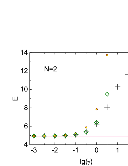
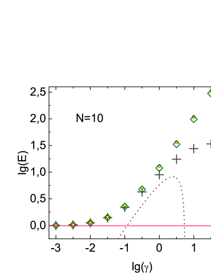
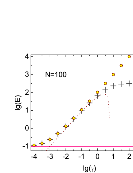
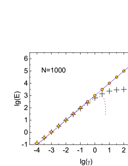
Fig. 3: [Color online] The dependence of the ground-state energy $E$ on $\gamma$ calculated in various models for $\bar{\rho}=1$ and $N=2$, $10$, $100$, $1000$: $E_{\mathrm{GP}}$ (circles), $E_{\mathrm{GP_{N}}}$ (diamonds), the exact energy $E_{\mathrm{Bethe}}$ (Eqs. (56) and (57) with $n_{j\leq N}=1$, crosses), and the Bogoliubov energy $E_{\mathrm{Bog}}=N\bar{\rho}^{2}\gamma\left(1-\frac{4\sqrt{\gamma}}{3\pi}\right)$ (dotted curve). The solid lines in panels $N=2$, $10$, $100$ correspond to the ground-state energy of $N$ free particles, $E=N(\pi/L)^{2}$, and in panel $N=1000$ to the curve $E=N\bar{\rho}^{2}\gamma$. In panels $N=2$ and $10$, the circles and diamonds are indistinguishable at $\lg{\gamma}\leq-1$. In panels $N=100$ and $1000,$ the curve $E_{\mathrm{GP_{N}}}(\gamma)$ would be very close to $E_{\mathrm{GP}}(\gamma)$ and therefore is not shown.

In the GP approach ($1-N^{-1}\rightarrow 1$), Eqs. (49) and (50) possess scaling properties: they do not change if $\gamma$ and $N$ vary provided $\gamma N^{2}=\mathrm{const}$. That is why the coefficients $g_{l}$ for such pairs $(\gamma,N)$ are identical. The particle density profiles $\rho(x)$ are also the same for them if $\bar{\rho}$ are the same. However, the energies $E_{GP}$ (53) are different for such $(\gamma,N)$ pairs.

4.2 Ground state energy

In this subsection, we find the energies $E_{\mathrm{GP}}$ and $E_{\mathrm{GP_{N}}}$ for the condensate ground state (formula (53) with $j_{0}=1$, $\hbar=2m=1$) and analyze their dependences on $N$, $\bar{\rho}$, and $\gamma$. We also compare $E_{\mathrm{GP}}$ and $E_{\mathrm{GP_{N}}}$ with the exact energy $E_{\mathrm{Bethe}}$ obtained from Eqs. (56), (57).

The dependence $E(\gamma)$ calculated for $N=2$, $10$, $100$, $1000$ is shown in Fig. 3. If $\gamma=0$, the ground state corresponds to $N$ free particles with the total energy $E=N(\pi/L)^{2}$. As one can see from the figures, the energies $E_{\mathrm{GP}}$ and $E_{\mathrm{GP_{N}}}$ are close to the energy of free particles if $\gamma$ is small. The larger $N$, the smaller $\gamma$ at which such a nearness of energy values takes place (because as $N$ increases, the potential energy increases faster than the kinetic one). At $\gamma\rightarrow\infty$, the exact solution $E_{\mathrm{Bethe}}$ tends to the limit of impenetrable bosons (for $N\rightarrow\infty$, this is $E_{\mathrm{Bethe}}=N\pi^{2}n^{2}/3$ [47]). Therefore, the curve $E_{\mathrm{Bethe}}(\gamma)$ saturates at $\gamma\gg 1$. In this case, the energies $E_{\mathrm{GP}}$ and $E_{\mathrm{GP_{N}}}$ differ strongly from the exact energy. However, if $\gamma\lesssim 0.1$, the energies $E_{\mathrm{GP}}$ and $E_{\mathrm{GP_{N}}}$ are close to the exact energy $E_{\mathrm{Bethe}}$ (we verified it for $\bar{\rho}=0.1$, $1$, and $10$). Moreover, for $N\gtrsim 100$, the energies $E_{\mathrm{GP}}$ and $E_{\mathrm{GP_{N}}}$ are close to the Bogoliubov ground-state energy if $\gamma$ is small but not too small.

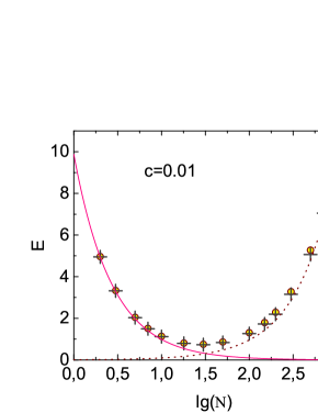
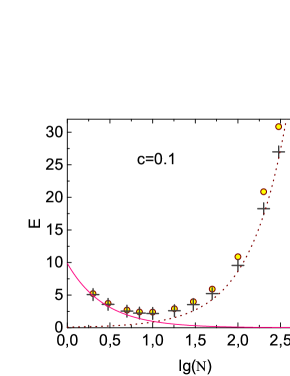
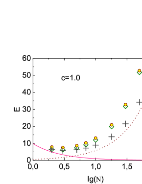
Fig. 4: [Color online] The dependence of the ground-state energy $E$ on $N$ calculated in different models for $\bar{\rho}=1$ and $c=0.01$, $0.1$, $1$: $E_{\mathrm{GP}}$ (circles), $E_{\mathrm{GP_{N}}}$ (diamonds), the exact energy $E_{\mathrm{Bethe}}$ (crosses), the Bogoliubov energy $E_{\mathrm{Bog}}=N\bar{\rho}^{2}\gamma\left(1-\frac{4\sqrt{\gamma}}{3\pi}\right)$ (solid curve). In panels $c=0.01$ and $0.1$, the curve $E_{\mathrm{GP_{N}}}(N)$ is not shown because it is very close to $E_{\mathrm{GP}}(N)$.

The dependence $E(N)$ for different $\gamma$ is shown in Fig. 4. From the dependence for $c=1$, one can see that the energy $E_{\mathrm{GP_{N}}}$ is close to $E_{\mathrm{Bethe}}$ even for a fairly large $\gamma$ ($\gamma=1$) if $N=2$ or $3$, but $E_{\mathrm{GP}}$ differs appreciably from $E_{\mathrm{Bethe}}$ for $\gamma=1$ and any $N$. At $\gamma=0.1$ the energies $E_{\mathrm{GP}}$ and $E_{\mathrm{GP_{N}}}$ are close to $E_{\mathrm{Bethe}}$ if $N\lesssim 100$. Finally, at $\gamma=0.01$, the energies $E_{\mathrm{GP}}$, $E_{\mathrm{GP_{N}}}$ and $E_{\mathrm{Bethe}}$ are close to each other for all $N$.

For all cases shown in the figures and not shown, the energy $E_{\mathrm{GP_{N}}}$ is closer to the exact energy $E_{\mathrm{Bethe}}$ than the energy $E_{\mathrm{GP}}$, for all values of the parameters. In this case, for $N\gg 1$ the energies $E_{\mathrm{GP}}$ and $E_{\mathrm{GP_{N}}}$ are very close to each other, whereas for $N\lesssim 10$ they are appreciably different, with $E_{\mathrm{GP_{N}}}$ being much closer to $E_{\mathrm{Bethe}}$.

Note the following interesting feature. One can see in panel $c=0.01$ in Fig. 4 that the condensate is close to the system of free particles when $N\lesssim 10$, and to Bogoliubov’s system when $N\gtrsim 300$. For $N\sim 30\div 100$, the system has already left the free particle regime but has not yet entered Bogoliubov’s one; in this case, the energies $E_{\mathrm{GP}}$ and $E_{\mathrm{GP_{N}}}$ are close to the exact energy $E_{\mathrm{Bethe}}$. That is, for $N\simeq 30$–$100$ structure (3) seems to work fairly well, whereas the interaction between the particles manifests itself more in the change of the form of $\Phi(x)$ rather than in interparticle correlations.

4.3 Particle density profile for the ground state

The local particle density for a 1D system of $N$ bosons in the state $\Psi(x_{1},\ldots,x_{N})$ is defined by the formula

$$\rho(x)=N\int dx_{2}\ldots dx_{N}|\Psi(x,x_{2},\ldots,x_{N})|^{2}.$$ (58)

For $N$ free particles being in the ground state $\Psi(x_{1},\ldots,x_{N})=\prod_{j=1,\ldots,N}\sqrt{2/L}\sin{(\pi x_{j}/L)}$, it gives

$$\rho(x)=2\bar{\rho}\sin^{2}{(\pi x/L)},\quad\bar{\rho}=N/L.$$ (59)

In the GP_N approach with the condensate ansatz (3), we obtain $\rho(x)=N|\psi(x,t)|^{2}$ with the normalization $\int_{0}^{L}dx|\psi(x,t)|^{2}=1$. For the stationary solution (38) with normalization (42), formula (58) gives

$$\rho(x)=|\Phi(x)|^{2},$$ (60)

where $\Phi(x)$ is the wave function from the GP_N equation (40). The operator GP_N approach also leads to (60): $\hat{\Psi}(\mathbf{r},t)=\hat{a}_{0}\Psi(\mathbf{r},t)/\sqrt{N}$, $\rho(x)=\langle\hat{\Psi}^{+}(x,t)\hat{\Psi}(x,t)\rangle_{T=0}=\langle\hat{N}_{0}\rangle_{T=0}|\Psi(x,t)|^{2}/N=|\Psi(x,t)|^{2}=|\Phi(x)|^{2}$ (here $\langle\hat{A}\rangle_{T=0}=\int dx_{1}\ldots dx_{N}\Psi_{N}^{\ast}\hat{A}\Psi_{N}=\langle N|\hat{A}|N\rangle$). Similarly, within the GP approach we find $\hat{\Psi}(x,t)=\Psi(x,t)$ and $\rho(x)=\langle\hat{\Psi}^{+}(x,t)\hat{\Psi}(x,t)\rangle_{T=0}=|\Psi(x,t)|^{2}=|\Phi(x)|^{2}$.

Let us determine $\rho(x)$ for the GP and GP_N approaches on the basis of Eqs. (44), (49), (50), and (60). The results of numerical analysis are depicted in Figs. 6 and 6. The GP and GP_N curves $\rho(x)$ are close to each other and would be visually indistinguishable. Therefore, only the GP_N curves are plotted.

Figure 6 demonstrates the $\rho(x)$-profile for $\gamma=0.01$ and different $N$. The curves $\rho(x)$ for $N=10$ and $N=30$ are similar to the curve for $N=2$ and contain no intervals with a constant particle density $\rho(x)=\mathrm{const}$. Such $\rho(x)$ are close to those for free particles. On the contrary, for $N\gtrsim 100,$ the profile $\rho(x)$ contains a large section where the particle density is constant, which testifies that the collective properties of the system manifest themselves at $N\gtrsim 100$. Note that the profiles $\rho(x)$ obtained in the GP and GP_N approaches for $\gamma=0.01$, $\bar{\rho}=1$, $N=2$ coincide with high accuracy with the profile $\rho(x)$ found by the Bethe ansatz (see Fig. 6).

Fig. 5: [Color online] Particle density profiles $\rho(x)$ in the ground state calculated for $\gamma=0.01$, $\bar{\rho}=1$, and various $N$: $\rho(x)$, obtained from the GP_N equation with $N=2$ (circles), $10$ (diamonds), $30$ (triangles), $100$ (asterisks), $1000$ (squares); the exact Bethe-ansatz solution for $N=2$ (dotted curve). The solid line marks the density profile $\rho(x)=2\bar{\rho}\sin^{2}{(\pi x/L)}$ for a system of any number ($N\geq 1$) of free particles with $\bar{\rho}=1$. The solid and dotted curves are almost indistinguishable from each other.

Fig. 6: [Color online] Particle density profiles $\rho(x)$ in the ground state calculated within the GP_N approach for $N=1000$, $\bar{\rho}=1$, and various $\gamma$: $\gamma=10^{-8}$ (diamonds), $10^{-6}$ (circles), $10^{-4}$ (triangles), $10^{-2}$ (squares), and $1$ (asterisks). The solid curve is the density profile $\rho(x)=2\bar{\rho}\sin^{2}{(\pi x/L)}$ for a system of free particles with $\bar{\rho}=1$.

Figure 6 shows the profiles $\rho(x)$ for $N=1000$ and different $\gamma$. Let us introduce the half-width $\eta$ of the wall layer; this parameter is equal to the smallest coordinate $x$ for which $\rho(x)=\rho(L/2)/2$. Numerical analysis showed that for $N=2$ and $\gamma\lesssim 1$, the quantity $\eta$ is practically independent of $\gamma$ and is equal to $\eta\approx L/4$. For $N=30$ and $0.1\lesssim\gamma\lesssim 1$, $\eta$ considerably depends on $\gamma$. And for $N=1000$ and $N^{-2}\ll\gamma\lesssim 1$, we have $\eta\approx\frac{1}{\bar{\rho}\sqrt{\gamma}}$ (a close estimate $\eta\approx\frac{\pi}{2\bar{\rho}\sqrt{\gamma}}$ was obtained in [46]). For $\gamma N^{2}\lesssim 1$ and any $N\geq 2$, the interval with the constant particle density disappears, and the system is in the near-free particle regime. In this case, the dependence $\rho(x)$ for $N$ interacting bosons is close to dependence (59) for free bosons, and the concept of the wall layer partly loses its meaning, although we may assume that $\eta=L/4$.

4.4 Near-free particle regime

The regime of near-free particles corresponds to the condition $\gamma N^{2}\lesssim 1$. For $N\gg 1$, this relation corresponds to ultraweak coupling, $\gamma\lesssim N^{-2}$. In this case, the solutions $|k_{j}|$ of Gaudin’s equations (57) have specific properties, and the ground state energy is approximately determined by the formula [48, 49]

$$E_{af}\approx\frac{N\pi^{2}}{L^{2}}+\frac{3(N-1)\gamma\bar{\rho}^{2}}{2}.$$ (61)

For example, for $N=1000$, $\bar{\rho}=1$, and $\gamma=10^{-8}$, we have $E_{af}=0.0098845894\equiv N\pi^{2}/L^{2}+0.000014985$, $E_{\mathrm{GP}}=0.0098846031\equiv N\pi^{2}/L^{2}+0.0000149987$, and $E_{\mathrm{GP_{N}}}=0.0098845881376\equiv N\pi^{2}/L^{2}+0.000014983738$. The exact solution is $E_{\mathrm{Bethe}}=0.009884588128\equiv N\pi^{2}/L^{2}+0.000014983728$.

In Fig. 7 the values of $\frac{E_{\mathrm{GP}}-E_{\mathrm{Bethe}}}{E_{\mathrm{Bethe}}}$ and $\frac{E_{\mathrm{GP_{N}}}-E_{\mathrm{Bethe}}}{E_{\mathrm{Bethe}}}$ are plotted for different $\gamma$ and $N$ for $\bar{\rho}=1$. Since $E_{\mathrm{Bethe}}$ is the exact solution, Fig. 7 illustrates the accuracy of the GP and GP_N approaches. It is easy to see that for $\gamma N^{2}\lesssim 1$, i.e. in the near-free particle regime, the GP_N approach is in much better agreement with the exact one than the GP approach.

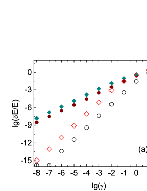
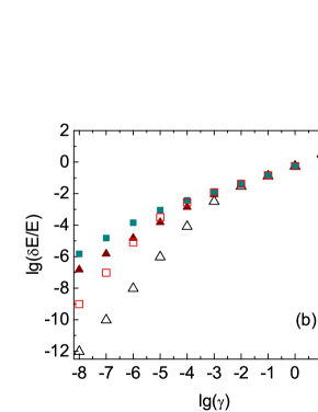
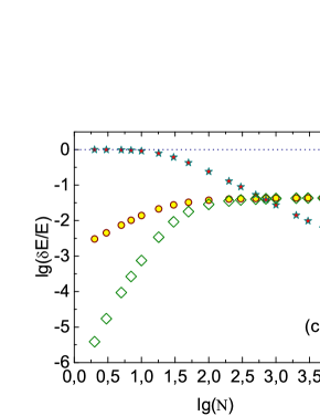
Fig. 7: [Color online] Comparison of the accuracy of the GP and GP_N approaches for $\bar{\rho}=1$. (a) $\gamma$-dependences of the ratio $\frac{E_{\mathrm{GP}}-E_{\mathrm{Bethe}}}{E_{\mathrm{Bethe}}}$ for $N=10$ (solid diamonds) and $N=2$ (solid circles), and the ratio $\frac{E_{\mathrm{GP_{N}}}-E_{\mathrm{Bethe}}}{E_{\mathrm{Bethe}}}$ for $N=10$ (hollow diamonds) and $N=2$ (hollow circles). (b) $\gamma$-dependences of the ratio $\frac{E_{\mathrm{GP}}-E_{\mathrm{Bethe}}}{E_{\mathrm{Bethe}}}$ for $N=100$ (solid diamonds) and $N=1000$ (solid circles), and the ratio $\frac{E_{\mathrm{GP_{N}}}-E_{\mathrm{Bethe}}}{E_{\mathrm{Bethe}}}$ for $N=100$ (hollow diamonds) and $N=1000$ (hollow circles). (c) Dependences of the ratios $\frac{E_{\mathrm{GP}}-E_{\mathrm{Bethe}}}{E_{\mathrm{Bethe}}}$ (circles), $\frac{E_{\mathrm{GP_{N}}}-E_{\mathrm{Bethe}}}{E_{\mathrm{Bethe}}}$ (diamonds), and $\frac{E_{\mathrm{Bethe}}-E_{\mathrm{Bog}}}{E_{\mathrm{Bethe}}}$ (asterisks) on $N$ for $c=0.01$. Here $E_{\mathrm{Bog}}=N\bar{\rho}^{2}\gamma\left(1-\frac{4\sqrt{\gamma}}{3\pi}\right)$ is the Bogoliubov ground-state energy of the 1D system of $N$ point bosons. The dotted line marks the zero level, $\lg{(\delta E/E)}=0$.

5 Comparison of the GP and GP_N approaches

Fig. 7 shows several patterns of relationships. First, both approaches reproduce the exact energy $E_{\mathrm{Bethe}}$ well for all $N\geq 2$ if $\gamma\lesssim 0.1$. Second, the GP and GP_N approaches give similar results for large $N$. However, for small $N$, the GP_N solutions agree much better, than the GP ones, with the exact solutions. For example, for $N=2$, $\bar{\rho}=1$, $\gamma=10^{-3}$, the estimates $\frac{E_{\mathrm{GP}}-E_{\mathrm{Bethe}}}{E_{\mathrm{Bethe}}}\approx 10^{-3.5}\sim\gamma$ and $\frac{E_{\mathrm{GP_{N}}}-E_{\mathrm{Bethe}}}{E_{\mathrm{Bethe}}}\approx 10^{-7.4}\sim\gamma^{2.5}$ hold, whereas for $N=2$, $\bar{\rho}=1$, $\gamma=10^{-7}$ we have $\frac{E_{\mathrm{GP}}-E_{\mathrm{Bethe}}}{E_{\mathrm{Bethe}}}\approx 10^{-7.5}\sim\gamma$ and $\frac{E_{\mathrm{GP_{N}}}-E_{\mathrm{Bethe}}}{E_{\mathrm{Bethe}}}\approx 10^{-15.7}\sim\gamma^{2.2}$. In the latter case, $E_{\mathrm{GP}}=4.9348025$, $E_{\mathrm{GP_{N}}}=4.9348023505446781$, and $E_{\mathrm{Bethe}}=4.9348023505446772$. That is, for $\gamma=10^{-7}$ the relative error of the GP_N solution is about $10^{-16}$. This is amazing accuracy!

A more general property holds: the GP_N approach works much better than the GP one in the near-free particle regime ($\gamma N^{2}\lesssim 1$), which corresponds to small $N$ ($N\lesssim\gamma^{-1/2}$) or small $\gamma$ ($\gamma\lesssim N^{-2}$). Why? In our opinion, this is a result of the following: It is natural to expect that every near-free boson with high probability is in the condensate, for any $N\geq 2$. Therefore, ansätze (3), (6), and $\hat{\Psi}(x,t)=\Psi(x,t)$ are good approximations. Since ansätze (3) and (6) are somewhat more accurate than the c-number ansatz $\hat{\Psi}(x,t)=\Psi(x,t)$, the GP_N approach turns out to be more accurate than the GP one.

It is commonly believed that the GP approach works only for large $N$ because the approximation $\hat{\Psi}(x,t)=\Psi(x,t)$ is reasonable only when $N\gg 1$. In point of fact, the GP approach works even better for small $N$ than for large $N$ (see Fig. 7). This surprising property appears to be due to the fact that the GP equation is simply close to the GP_N one, which describes few-particle systems with high accuracy.

In turn, the following question arises: Why is the GP_N equation works better in the case of small $N$? The evident answer is that the role of two- and many-particle correlations is less for small $N$ (such correlations are not taken into account in ansätze (3), (6)). More information can be obtained from the diagonal expansion of the single-particle density matrix

$$F_{1}(x,x^{\prime})=\sum\limits_{j=1}^{\infty}\lambda_{j}\phi_{j}^{\ast}(x^{\prime})\phi_{j}(x),$$ (62)

where $\lambda_{j}$ are the occupation numbers of the single-particle states $\phi_{j}(x)$, and $\phi_{j}(x)$ form the complete collection of orthonormal functions. Condensate ansätze (3) and (6) describe the system well only if $\sqrt{N}\phi_{1}(x)$ is close to the solution $\Phi(x)$ of the GP_N equation, and the relations $\lambda_{1}\simeq N$, $\lambda_{j>1}\ll N$ hold (in his case, $\lambda_{1}+\lambda_{2}+\ldots+\lambda_{\infty}=N$). We suppose that $(\frac{\lambda_{1}(\gamma)}{N}|_{N\leq 10})>(\frac{\lambda_{1}(\gamma)}{N}|_{N\geq 100})$ for $\gamma\lesssim 0.1$. If so, then the role of two- and many-particle correlations is less for $N\lesssim 10$ than for $N\gtrsim 100$.

Next, one can see from Fig. 7c that the Bogoliubov energy $E_{\mathrm{Bog}}$ for large $N$ is closer to the exact energy $E_{\mathrm{Bethe}}$ than the energies $E_{\mathrm{GP}}$ and $E_{\mathrm{GP_{N}}}$. That is, the Bogoliubov method describes the ground state of the system with large $N$ more accurately than the GP and GP_N approaches do. This property shows that taking into account above-condensate atoms—which is done in the Bogoliubov model, but not in the GP and GP_N approaches—is significant.

In order to better understand the properties of the system, it is necessary to find the density matrix (62) and an equation for the condensate in the approximation that accurately takes into account the above-condensate atoms (or, equivalently, two- and many-particle correlations).

6 Concluding remarks

We have shown that the condensate ansätze (3) and (6) lead to a nonlinear Schrödinger equation (the GP_N equation), which differs from the standard Gross-Pitaevskii (GP) equation by the additional factor $\left(1-1/N\right)$. We have analysed the ground state of the system and compared the solutions of the GP and GP_N equations with the exact solutions. The analysis showed that both equations describe well a Bose system with any number of particles $N\geq 2$, if the coupling is weak: $\gamma\lesssim 0.1$ (we considered the mean particle densities $n=0.1$, $1$, and $10$). This result significantly extends the conventional view that the Gross-Pitaevskii equation is applicable only in the case of $N\gg 1$.

In the case of the near-free particle regime, $\gamma N^{2}\lesssim 1$, the GP_N equation describes the Bose system much better than the standard Gross-Pitaevskii equation does. The condition $\gamma N^{2}\lesssim 1$ can be written as $\gamma\lesssim N^{-2}$ or $N\lesssim\gamma^{-1/2}$, which corresponds to ultraweak coupling or small $N$, respectively. These properties and the analysis in [29, 30] indicate that phonons in a superfluid Bose gas and helium-II are not Goldstone bosons (see section 2).

Since the GP_N equation describes a few-boson system with high accuracy, it is worth extending the concept of the condensate to systems with small $N$, using the following criterion: if $\lambda_{1}\gg\lambda_{2}+\ldots+\lambda_{N}$ in (62), then state 1 is a condensate state, whereas other states are not. For an ideal gas, all $\lambda_{j}$ are integers, and this criterion gives $\lambda_{1}=N;\lambda_{2}=\ldots=\lambda_{N}=0$.

Interestingly, the GP and GP_N equations work well for all $N$ and $\gamma\lesssim 0.1$, although they completely ignore two-particle and higher order correlations. This property means that these correlations are weak when $\gamma\lesssim 0.1$.

To describe a system of $N$ spinless interacting bosons, several methods have been proposed (below we cite only some references, according to our subjective view). These are analytical methods for systems with $N\gg 1$ and weak coupling [3, 22, 50, 51, 52, 53, 54]; numerical methods for systems with $N=2\div 10$ and any, weak or strong, coupling (here different expansions in basis functions are used) [8, 55, 56, 57]; and Monte Carlo methods for systems with $N\sim 10\div 100$ and arbitrary coupling [58, 59]. The exactly solvable approach describes 1D systems of $N\geq 2$ point bosons, for arbitrary coupling [42, 41, 60, 61]. The GP and GP_N equations provide one more analytical method for systems with $N\geq 2$ (in this case, the GP_N equation more accurately describes systems with $2\leq N\lesssim 100$). To our knowledge, the ground state of Bose systems with $10\lesssim N\lesssim 100$ can be accurately described only by the Monte Carlo method and the GP_N approach. Thus, the factor $\left(1-1/N\right)$ makes it possible to accurately describe Bose systems with small $N$ using the Gross-Pitaevskii equation.

Appendix: Proof that $\Phi(x)$ is real

Let us show that any solution $\Phi(x)$ of Eq. (39) with zero BCs (41) can be written in the real form.

Let a solution of Eq. (39) be complex, $\Phi(x)=\Phi_{1}(x)+i\Phi_{2}(x)$, where $\Phi_{1}(x)$ and $\Phi_{2}(x)$ are real functions. Then Eq. (39) can be written as two equations:

$$\epsilon\Phi_{1}=-\frac{\hbar^{2}}{2m}\frac{\partial^{2}\Phi_{1}}{\partial x^{2}}+2c(\Phi_{1}^{2}+\Phi_{2}^{2})\Phi_{1},$$ (63)

$$\epsilon\Phi_{2}=-\frac{\hbar^{2}}{2m}\frac{\partial^{2}\Phi_{2}}{\partial x^{2}}+2c(\Phi_{1}^{2}+\Phi_{2}^{2})\Phi_{2}.$$ (64)

Multiplying Eq. (63) by $\Phi_{2}(x)$ and Eq. (64) by $\Phi_{1}(x)$, and subtracting the results, we obtain the equation

$$\Phi_{2}\frac{\partial^{2}\Phi_{1}}{\partial x^{2}}=\Phi_{1}\frac{\partial^{2}\Phi_{2}}{\partial x^{2}}.$$ (65)

Let us expand $\Phi_{1}(x)$ and $\Phi_{2}(x)$ in sine series,

$$\Phi_{1}(x)=\sum\limits_{j=1,2,\ldots,\infty}a_{j}\sqrt{2/L}\cdot\sin(k_{j}x),\quad\Phi_{2}(x)=\sum\limits_{j=1,2,\ldots,\infty}b_{j}\sqrt{2/L}\cdot\sin(k_{j}x),$$ (66)

where $k_{j}=\pi j/L$. Then Eq. (65) can be written in the form

$$\sum\limits_{j_{1}j_{2}=1,2,\ldots,\infty}k_{j_{1}}^{2}(b_{j_{1}}a_{j_{2}}-b_{j_{2}}a_{j_{1}})\sin(k_{j_{1}}x)\sin(k_{j_{2}}x)=0,$$ (67)

or

$$(1/2)\sum\limits_{j_{1}j_{2}=1,2,\ldots,\infty}k_{j_{1}}^{2}(b_{j_{1}}a_{j_{2}}-b_{j_{2}}a_{j_{1}})[\cos(k_{j_{1}-j_{2}}x)-\cos(k_{j_{1}+j_{2}}x)]=0.$$ (68)

Using the formulae

$$\cos(k_{j}x)=\sum\limits_{p=1,2,\ldots,\infty}c_{j}^{p}\sin(k_{p}x),$$ (69)

$$c_{j}^{p}=\left[\begin{array}[]{ccc}0&\ \mbox{for even}\ p-j,&\\ \frac{2}{\pi}\left(\frac{1}{p-j}+\frac{1}{p+j}\right)&\mbox{for odd}\ p-j,&\end{array}\right.$$ (70)

let us write Eq. (68) as follows:

$$(1/2)\sum\limits_{j_{1}j_{2}=1,2,\ldots,\infty}k_{j_{1}}^{2}(b_{j_{1}}a_{j_{2}}-b_{j_{2}}a_{j_{1}})\sum\limits_{p=1,2,\ldots,\infty}(c_{j_{1}-j_{2}}^{p}-c_{j_{1}+j_{2}}^{p})\sin(k_{p}x)=0.$$ (71)

Let the function $\Phi_{1}(x)$ be known, and $\Phi_{2}(x)$ unknown. Since the functions $\sin(k_{p}x)$ are independent, we obtain from Eq. (71) the system of equations for the unknown coefficients $b_{j}$:

$$\sum\limits_{j_{1}j_{2}=1,2,\ldots,\infty}k_{j_{1}}^{2}(b_{j_{1}}a_{j_{2}}-b_{j_{2}}a_{j_{1}})(c_{j_{1}-j_{2}}^{p}-c_{j_{1}+j_{2}}^{p})=0,\quad p=1,2,\ldots,\infty.$$ (72)

Such a system of linear homogeneous equations for $b_{j}$, $\sum_{j}A_{pj}b_{j}=0$, always has a zero solution: $b_{j}=0$ for all $j=1,2,\ldots,\infty$. If the determinant of the matrix $A_{pj}$ is zero, then this system of equations also has one nonzero solution, namely, $b_{j}\neq 0$ for at least two $j$’s. It is easy to see that the quantities $b_{j}=ra_{j}$, where $r$ is the same for all $j=1,2,\ldots,\infty$, provide a solution of system (72). So, we obtain two possible solutions: $\Phi_{2}(x)=r\Phi_{1}(x)$ and $\Phi_{2}(x)=0$. In both cases, $\Phi(x)=\Phi_{1}(x)+i\Phi_{2}(x)=\mathrm{const}\cdot\Phi_{1}(x)$. Therefore, we can consider the function $\Phi(x)$ in Eq. (39) to be real. This analysis can be easily generalized to two- and three-dimensional cases.

References

- [1] Gross E P Phys. Rev. 106 161 (1957)
- [2] Gross E P Ann. Phys. 4 57 (1958)
- [3] Bogoliubov N N J. Phys. USSR 11 23 (1947)
- [4] Pitaevskii L P Sov. Phys. JETP 13 451 (1961)
- [5] Gross E P Nuovo Cimento 20 454 (1961) https://doi.org/10.1007/BF02731494
- [6] Leggett A G Rev. Mod. Phys. 73, 307 (2001) https://doi.org/10.1103/RevModPhys.73.307
- [7] Pethick C J and Smith H Bose–Einstein Condensation in Dilute Gases (Cambridge University Press, New York, 2008)
- [8] Blume D Rep. Prog. Phys. 75 046401 (2012) https://doi.org/10.1088/0034-4885/75/4/046401
- [9] Pitaevskii L and Stringari S Bose-Einstein Condensation and Superfluidity (Oxford University Press, New York, 2016) ch 5
- [10] Cornell E A and Wieman C E Rev. Mod. Phys. 74 875 (2002)
- [11] Ketterle W Rev. Mod. Phys. 74 1131 (2002)
- [12] Fetter A L and Walecka J D Quantum Theory of Many-Particle Systems (McGraw-Hill, New York, 1971)
- [13] Noziéres P and Pines D The Theory of Quantum Liquids, vol. II (CRC Press, New York, 2018)
- [14] Lieb E H, Seiringer R, Solovej J P and Yngvason J The Mathematics of the Bose Gas and its Condensation (Birkhäuser-Verlag, Basel, 2005)
- [15] Esry B D Many-body effects in Bose-Einstein condensates of dilute atomic gases, PhD Thesis (University of Colorado, Boulder, 1997)
- [16] Salasnich L Int. J. Mod. Phys. B 14 1 (2000) https://doi.org/10.1142/S0217979200000029
- [17] Blume D and Greene C H Phys. Rev. A 63 063601 (2001) https://doi.org/10.1103/PhysRevA.63.063601
- [18] Tomchenko M arXiv:2311.03176 [cond-mat.quant-gas]
- [19] Carr L D, Clark C W and Reinhardt W P Phys. Rev. A 62 063610 (2000). https://doi.org/10.1103/PhysRevA.62.063610
- [20] Petrov D S, Gangardt D M and Shlyapnikov G V J. Phys. IV Fr. 116 5 (2004)
- [21] Bouchoule I, van Druten N J and Westbrook C I arXiv:0901.3303 [physics.atom-ph]
- [22] Vakarchuk I A and Yukhnovskii I R Theor. Math. Phys. 40 626 (1979) https://doi.org/10.1007/BF01019246
- [23] Gross E P Ann. Phys. 20 44 (1962) https://doi.org/10.1016/0003-4916(62)90115-X
- [24] Woo C-W Phys. Rev. A 6 2312 (1972) https://doi.org/10.1103/PhysRevA.6.2312
- [25] Feenberg E Ann. Phys. 84 128 (1974) https://doi.org/10.1016/0003-4916(74)90296-6
- [26] Wu T T J. Math. Phys. 2 105 (1961) https://doi.org/10.1007/BF01019246
- [27] Landau L D and Lifshitz E M Quantum Mechanics. Non-Relativistic Theory (Pergamon Press, New York, 1980)
- [28] Bogoliubov N N Lectures on Quantum Statistics, vol. 2: Quasi-Averages (Gordon and Breach, New York, 1970)
- [29] Gardiner C W Phys. Rev. A 56 1414 (1997) https://doi.org/10.1103/PhysRevA.56.1414
- [30] Girardeau M D Phys. Rev. A 58 775 (1998) https://doi.org/10.1103/PhysRevA.58.775
- [31] Anderson P W Basic notions of condensed matter physics (Benjamin/Cummings, Menlo Park CA, 1984) ch 2
- [32] Forster D Hydrodynamic fluctuations, broken symmetry, and correlation functions (CRC Press, Boca Raton FL, 2018) ch 7, 10
- [33] Powell B J Contemporary Physics 61 96 (2020) https://doi.org/10.1080/00107514.2020.1832350
- [34] Goldstone J, Salam A and Weinberg S Phys. Rev. 127 965 (1962) https://doi.org/10.1103/PhysRev.127.965
- [35] Andersen K H, Stirling W G, Scherm R, Stunault A, Fak B, Godfrin H and Dianoux A J J. Phys.: Condens. Matter 6 821 (1994) https://doi.org/10.1088/0953-8984/6/4/003
- [36] Andersen K H and Stirling W G J. Phys.: Condens. Matter 6 5805 (1994) https://doi.org/10.1088/0953-8984/6/30/004
- [37] Blagoveshchenskii N M, Puchkov A V, Skomorokhov A N, Bogoyavlenskii I V and Karnatsevich L V Low Temp. Phys. 23 374 (1997) https://doi.org/10.1063/1.593381
- [38] Gibbs M R, Andersen K H, Stirling W G and Schober H J. Phys.: Condens. Matter 11 603 (1999) https://doi.org/10.1088/0953-8984/11/3/003
- [39] Kalinin I V, Lauter H and Puchkov A V JETP 105 138 (2007) https://doi.org/10.1134/S1063776107070291
- [40] Bethe H A Z. Phys. 71 205 (1931)
- [41] Lieb E H and Liniger W Phys. Rev. 130 1605 (1963)
- [42] Gaudin M Phys. Rev. A 4 386 (1971)
- [43] Gaudin M The Bethe Wavefunction (Cambridge University Press, Cambridge, 2014)
- [44] Syrwid A J. Phys. B: At. Mol. Opt. Phys. 54 103001 (2021) https://doi.org/10.1088/1361-6455/abd37f
- [45] Tomchenko M J. Phys. A: Math. Theor. 50 055203 (2017)
- [46] Tomchenko M D Ukr. J. Phys. 64 250 (2019) https://doi.org/10.15407/ujpe64.3.250
- [47] Girardeau M J. Math. Phys. 1 516 (1960)
- [48] Batchelor M T, Guan X W, Oelkers N and Lee C J. Phys. A: Math. Gen. 38 7787 (2005)
- [49] Tomchenko M J. Phys. A: Math. Theor. 48 365003 (2015)
- [50] Feynman R Phys. Rev. 94 262 (1954) https://doi.org/10.1103/PhysRev.94.262
- [51] Bogoliubov N N and Zubarev D N Sov. Phys. JETP 1 83 (1956)
- [52] Brueckner K Theory of Nuclear Structure (Methuen, London, 1959)
- [53] Vakarchuk I A and Yukhnovskii I R Theor. Math. Phys. 42 73 (1980) https://doi.org/10.1007/BF01019263
- [54] Pashitskii E A, Mashkevich S V and Vilchynskyy S I J. Low Temp. Phys. 134 851 (2004) https://doi.org/10.1023/B:JOLT.0000013206.08699.a2
- [55] Multidimensional Quantum Dynamics: MCTDH Theory and Applications ed H-D Meyer, F Gatti and G A Worth (Wiley-VCH, Weinheim, 2009)
- [56] Zinner N T EPJ Web of Conferences 113 01002 (2016) https://doi.org/10.1051/epjconf/201611301002
- [57] Sowiński T and Garćia-March M A Rep. Prog. Phys. 82 104401 (2019)
- [58] Schmidt K E and Ceperley D M Monte Carlo techniques for quantum fluids, solids and droplets, in Monte Carlo Methods in Condensed Matter Physics, ed K Binder, Topics in Applied Physics, vol 71 (Springer, Heidelberg, 1992) pp. 205–248 https://doi.org/10.1007/3-540-60174-0_7
- [59] Whitlock P A and Vitiello S A Quantum Monte Carlo Simulations of Solid 4He, in: Large-Scale Scientific Computing. LSSC 2005, ed I Lirkov, S Margenov and J Wasniewski, Lecture Notes in Computer Science, vol 3743 (Springer, Berlin, 2006) pp. 40–52 https://doi.org/10.1007/11666806_4
- [60] Lieb E H Phys. Rev. 130 1616 (1963) https://doi.org/10.1103/PhysRev.130.1616
- [61] Tomchenko M D Dopov. Nac. Akad. Nauk Ukr. No. 12 49 (2019) https://doi.org/10.15407/dopovidi2019.12.049