1 Introduction

The properties of many functional materials depend to a large extent on their structure and chemical composition. Hence, measuring both is mandatory in order to understand and improve their effective properties. An important class of materials are hetero-aggregates, which are compositions of at least two dissimilar classes of primary particles, called, for the sake of simplicity, particles from now on. Properties of hetero-aggregates can be quite different in comparison to aggregates that consist of monodisperse particles. A prominent example in applications concerned with photocatalysis are hetero-aggregates made of titanium dioxide (TiO2) and tungsten trioxide (WO3) [33, 40, 43]. The combination of both materials leads to aggregates with hetero-junctions, i.e., points at which two particles made from different materials touch. At such junctions, photogenerated electron-hole pairs are spatially separated, hindering their direct recombination, which results in a higher photocatalytic activity compared to pure TiO2 [25].

In order to accurately investigate the properties of hetero-aggregates with imaging techniques, it is essential to resolve the individual particles within the structure. A suitable tool for the characterization of hetero-aggregates, consisting of particles with radii of a few nanometers, is (scanning) transmission electron microscopy, (S)TEM. With a spatial resolution in the sub-nanometer regime, even the atomic structure can be investigated. However, in conventional STEM only two-dimensional (2D) projection images of the aggregates can be acquired while information about the third dimension is lost. This problem can be overcome using STEM tomography, where the sample is tilted with respect to the electron beam such that a series of projection images under various projection angles is acquired, see [28]. From this series of STEM projection images, the three-dimensional structure can be reconstructed, e.g., with iterative reconstruction techniques [12]. The major disadvantage of STEM tomography is the fact that acquisition of a single tilt series can take several hours, and thus, this method does hardly allow for the investigation of a large number of aggregates. Furthermore, many samples do not allow for such a long measurement as hetero-aggregates and nanoparticles can change their structure and arrangement during extensive exposure to the electron beam, hindering the reconstruction.

As opposed to STEM tomography, 2D STEM images can be acquired within a few seconds, allowing for the acquisition of several images of various aggregates in a reasonable amount of time. For this reason, it is desirable to use 2D STEM images in order to characterize the 3D morphology of aggregates. This can be achieved by training neural networks to predict structural properties of 3D hetero-aggeregates from 2D STEM images. However, the training of neural networks requires a broad database of pairs of differently structured hetero-aggregate and corresponding 2D STEM images. The experimental acquisition of such a database, i.e., the synthesis of differently structured aggregates and their imaging would be expensive in both time and resources. Alternatively, simulated image data can be used for training purposes, see [10] for a similar approach.

In the present paper, a stochastic 3D model for the generation of virtual aggregates and a physics-based STEM model for the simulation of corresponding 2D STEM images is combined in order to provide training data. In other words, methods of stochastic geometry [4] are utilized to derive a parametric model for the generation of a wide spectrum of virtual, but realistic aggregates. Additionally, the virtual structures are passed to a physics-based simulation tool in order to generate virtual scanning transmission electron microscopy (STEM) images. The preset parameters of the 3D model together with the simulated STEM images serve as a database for the training of convolutional neural networks, which can be used to predict the parameters of the underlying 3D model and, consequently, to predict 3D structures of hetero-aggregates from 2D STEM images. In literature, there are already CNN-based approaches that do not use stochastic geometry models to generate stochastically equivalent 3D structures from 2D images [19]. However, the presented approach aims to generate such digital shadows by combining a well-established parametric stochastic 3D model and a CNN-based approach. In order to use such a parametric stochastic 3D model to generate digital shadows of hetero-aggregates, appropriate values of the model parameters must be chosen. The focus of the present paper is on this calibration procedure, also called model fitting.

More specifically, it is investigated how convolutional neural networks (CNNs) [13, 16] can be used to determine the parameters of the stochastic 3D model and, consequently, to generate digital shadows of 3D aggregates, from 2D STEM images. CNNs are a type of artificial neural networks commonly used in image analysis and recognition tasks, see e.g. [22]. They consist of multiple layers of neurons that learn to recognize patterns and features in the input data through a calibration process, called training.

In conventional spatial stochastic modeling of complex 3D morphologies, the process of model fitting typically involves several steps, see for example [31, 42]. First, image data has to be acquired, preprocessed, and segmented. Subsequently, an appropriate model type is chosen, and its model parameters are adjusted accordingly using descriptive statistics of the segmented image data. However, the approach considered in the present paper differs from the classical one. On the one hand, the image data does not have to be segmented, which is advantageous since image segmentation can be a time-consuming complex task. Moreover, the model parameters are predicted by the neural networks directly, meaning that the descriptive statistics are not chosen by hand. This allows for the use of stochastic 3D models with parameters which are not easily estimatable from the image data.

In order to evaluate the performance of such a CNN-based approach, structural descriptors of aggregates drawn from the stochastic 3D model with preset parameter values are compared with structural descriptors of aggregates drawn from the 3D model with parameter values predicted by the CNN-based approach.

However, the structural similarity of the measured image data of aggregates and image data drawn from the fitted 3D model strongly depends on two factors, (i) the suitability of the chosen model type for the given data, and (ii) the ability of the selected CNN approach to determine the parameters of the stochastic 3D model from 2D STEM image data. More specifically, when analyzing measured image data of experimentally synthesized hetero-aggregates, there might not be any configuration of model parameters that results in a high-quality fit. In this case, the dissimilarities between the original image data and its digital shadows, generated by the fitted model, cannot necessarily be attributed to the fitting procedure, but rather to the inadequate choice of the model type. Thus, in the present paper, to be able to attribute these dissimilarities to an inadequate CNN approach, including data preprocessing, model architecture and learning procedure, the same stochastic 3D model is used as both the generator for the training data and the model to be fitted.

For an adequately designed CNN approach and adequately chosen type of the stochastic 3D model, the digital shadows drawn from the fitted 3D model should be statistically equivalent to experimentally synthesized aggregates in terms of their 3D structure and chemical composition. Then, these digital shadows can be used as geometry input of (spatially resolved) numerical modeling and simulation, to determine their functional properties, see e.g. [30, 34]. In this way, 3D imaging techniques like STEM tomography of the aggregates can be avoided in order to derive quantitative process-structure or structure-property relationships for hetero-aggregates. Note that by means of such relationships, optimized specifications of process parameters can be deduced, which lead to hetero-aggregates with desired structures and properties. Digital shadows used for structure-property optimization are also referred to as digital twins. Their implementation will be the subject of a forthcoming study.

The present work is organized as follows: In Section 2 the CNN-based approach is described to predict the 3D structure of hetero-aggregates from 2D STEM images. In particular, the generation of synthetic training data is explained which are used for the prediction of model parameters. Then, in Section 3, the results are presented which have been obtained for various aspects of model parameter prediction. Section 4 compares the methods developed in the present paper with analysis tools considered in the literature. Section 5 concludes.

2 Methods

This section provides details how the presented CNN-based approach is built for predicting the 3D structure of hetero-aggregates from 2D STEM images. It comprises two main steps. First, virtual but realistic STEM images are generated from simulated 3D image data. More specifically, synthetic aggregates are drawn from a stochastic 3D model with preset model parameters, where the latter describe the aggregation procedure simulated by the model and therefore influence structural properties of the generated aggregates. These aggregates are then used to generate corresponding STEM images by means of a physics-based simulation tool, see Figure 1a. Systematically varying the parameters of the stochastic 3D model provides a wide range of differently structured aggregates and their STEM images. In a second step, visualized in Figure 1b, the parameters of the stochastic 3D model together with the simulated STEM images serve as a database for the training of CNNs, in order to learn how to reconstruct the parameters of the stochastic 3D model from STEM images. For the reconstruction, initially, a CNN extracts features from STEM images which characterize the depicted structure of aggregates in an informative but not necessarily interpretable manner. Then, these features are utilized to predict our interpretable predefined model parameters. For more details, see Section 2.3. This approach is designed to allow for quick and accurate prediction of model parameters for real hetero-aggregates from measured STEM images and, consequently, to predict the 3D morphology of hetero-aggregates from 2D STEM images.

The quality of the predictor is evaluated with respect to the similarity between predefined and predicted model parameters. Recall that interpretable model parameters describe the aggregation procedure simulated by the stochastic model. Thus, a good match between predefined and predicted model parameters can already be an indication for a good structural match between aggregates generated by the model with predefined/predicted parameters. Nevertheless, some structural descriptors (i.e., quantities which characterize the structure of aggregates like hetero-coordination number) may be sensitive with respect to changes in the model parameters.

Therefore, the quality of the predictor is further evaluated by comparing structural descriptors of aggregates drawn from stochastic 3D models with pre-defined and predicted parameters, respectively, see Figure 1c,d. The structural descriptors considered in this paper, which are chosen due to their relevance in process engineering, are displayed in Table 1. They are complementary to the features, utilized in the model parameter prediction. Furthermore, these descriptors are interpretable and characterize the 3D structure of the aggregates (whereas the features describe the structure observed in 2D images).

descriptor	symbol
average cluster sizes of TiO2 particles	$S_{\mathrm{\ce{TiO2}}}$
hetero-coordination number	$Z_{\mathrm{hetero}}$
coordination number	$Z_{\mathrm{total}}$

Table 1: Structural descriptors used for evaluating the model parameter prediction. For formal definitions of the descriptors, see Section 3.4.

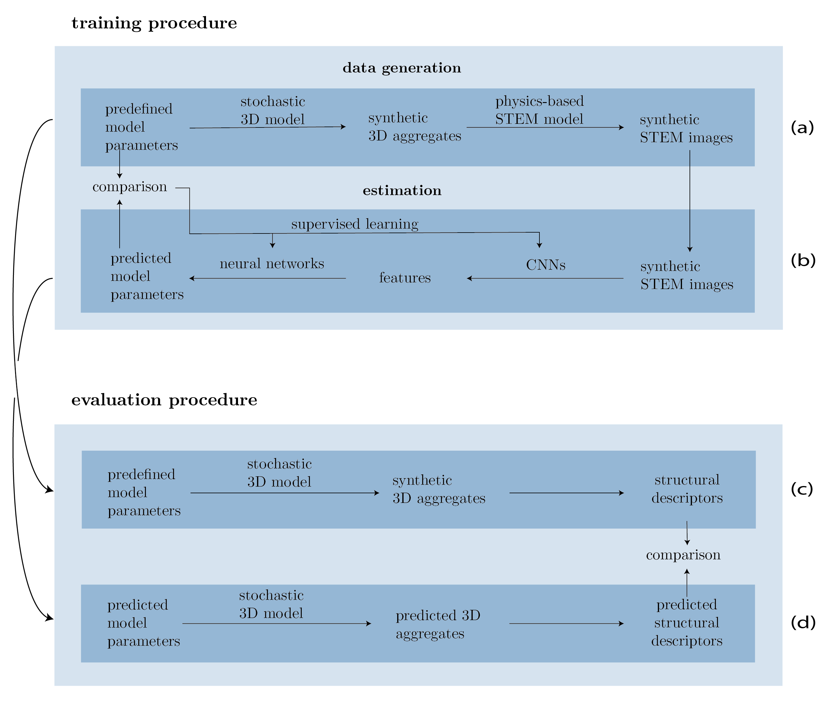
Figure 1: Workflow of the training and evaluation procedure.

2.1 Generation of synthetic training data

The use of synthetic training data requires careful attention to ensure that the artificially generated data accurately reflects particularities of experimentally measured data such that a regression model (e.g., a CNN) trained on synthetic data can be extended to new, real-world data. More precisely, if the generation of realistic data is successful, a network trained on this data can be used for applications on real-world data, and thus, reducing the amount of experimentally measured and labeled training data.

In the present study, synthetic training data was generated through a three-step process. First, virtual hetero-aggregates were generated using a stochastic 3D model. Then, using a physics-based simulation tool, STEM intensities were determined based on the material and thickness of the aggregates. Finally, virtual but realistic STEM images were computed by adding noise and other sources of variability to the previously determined STEM intensities. In the following, the stochastic 3D model is introduced and then more details about each of the data generation steps mentioned above is provided.

2.1.1 Stochastic 3D model

In this section, the stochastic 3D model is introduced, which will be used to generate a wide spectrum of virtual hetero-aggregates by varying the values of four different model parameters, denoted by $\theta_{\mathrm{D_{f}}},\theta_{\mathrm{\uprho}},\theta_{\mathrm{0}},\theta_{\mathrm{1}}$, where $\theta_{\mathrm{D_{f}}}\in(1,3),\theta_{\mathrm{\uprho}}\in(0,1)$, and $\theta_{\mathrm{0}},\theta_{\mathrm{1}}\in\mathbb{N}=\{1,2,\ldots\}$.

These model parameters control the fractal dimension, the mixing ratio, and clustering properties of the hetero-aggregates, respectively.

Throughout this paper, a spherical particle is defined as a triplet $p=(x,r,l)$ of particle position $x\in\mathbb{R}^{3}$, radius $r\in\mathbb{R}^{+}=(0,\infty)$ and label $l\in\{0,1\}$. Moreover, a hetero-aggregate $A$, consisting of $N$ particles for some fixed $N\in\mathbb{N}$, is a set of connected and non-overlapping spherical particles, i.e.,

$$A=\{p_{i}=(x_{i},r_{i},l_{i}):x_{i}\in\mathbb{R}^{3},\leavevmode\nobreak\ r_{i}\in\mathbb{R}^{+},\leavevmode\nobreak\ l_{i}\in\{0,1\},\leavevmode\nobreak\ 1\leq i\leq N\}.$$ (1)

In this context, two particles $p,p^{\prime}\in A$ are said to be connected if for some $j\in\{2,\ldots,N\}$ there is a set of indices $\{i_{1},\ldots,i_{j}\}\subset\{1,\ldots,N\}$ with $p=p_{i_{1}}$ and $p^{\prime}=p_{i_{j}}$, such that

$$\|x_{i_{k}}-x_{i_{k+1}}\|\leq 1.01(r_{i_{k}}+r_{i_{k+1}})\leavevmode\nobreak\ \text{ for all }k\in\{1,\ldots,j\}\,,$$ (2)

where $\|y\|=\sqrt{\sum_{k=1}^{3}y_{k}^{2}}$ denotes the Euclidean norm of $y=(y_{1},y_{2},y_{3})\in\mathbb{R}^{3}$. The prefactor $1.01$ in Eq. (2) represents the maximum distance of particles which is allowed to consider them to be in contact. It is determined to be $1\%$ of the sum of their radii. Moreover, two particles $p=(x,r,l),p^{\prime}=(x^{\prime},r^{\prime},l^{\prime})$ are said to be overlapping if the distance of their centers is smaller than the sum of their radii, i.e., $\|x-x^{\prime}\|<r+r^{\prime}$. The label $l$ of a particle $p=(x,r,l)$ determines its material. More precisely, in our case, a particle with label $l=0$ consists of $\ce{WO3}$, whereas a particle with label $l=1$ consists of $\ce{TiO2}$.

The mixing ratio $\rho$ of an aggregate $A$ is defined as its fraction of particles with label $l=0$, i.e.,

$$\rho(A)=\frac{\#\{p_{i}\in A\colon l_{i}=0\}}{\#A}\,,$$ (3)

where $\#$ denotes cardinality.

Notice the distinction in notation between $\theta_{\mathrm{\uprho}}$ and $\rho$ since these values are not necessarily equal. More precisely, the model parameter $\theta_{\mathrm{\uprho}}$ can be set to an arbitrary value in the interval $[0,1]$ and it primarily influences the distribution of the structural descriptor $\rho$ of aggregates generated with $\theta_{\mathrm{D_{f}}}$, as explained in more detail later on. Furthermore, the radius of gyration $R_{\mathrm{g}}>0$ of an aggregate $A$ is given by

$$R_{\mathrm{g}} =\sqrt{\frac{\sum_{i=1}^{N}m_{i}\cdot\|x_{i}-c_{0}\|^{2}}{\sum_{i=1}^{N}m_{i}}}\leavevmode\nobreak\ ,\quad\text{with}\leavevmode\nobreak\ \leavevmode\nobreak\ c_{0}=\frac{\sum_{i=1}^{N}m_{i}x_{i}}{\sum_{i=1}^{N}m_{i}}\,,$$ (4)

where $m_{1},\dots,m_{N}>0$ denote the particle masses and $c_{0}$ is the aggregate’s center of mass.

The stochastic 3D model described below is motivated by the idea that hetero-aggregates have a fractal-like structure [9, 27]. This fractal-like structure of an aggregate $A$ can be quantified by the so-called fractal dimension $D_{\mathrm{f}}$, given by

$$D_{\mathrm{f}}=\frac{\log\left(\frac{N}{k_{\mathrm{f}}}\right)}{\log\left(\frac{R_{\mathrm{g}}}{a}\right)}\,,\leavevmode\nobreak\$$ (5)

where $k_{\mathrm{f}}>0$ is a fractal prefactor, which is set to $1.3$, and $a=\frac{1}{N}\sum_{i=1}^{N}r_{i}$ is the mean radius of the particles. For example, aggregates with a fractal dimension $D_{\mathrm{f}}$ close to $1$ are arranged in a nearly straight line, whereas those with a fractal dimension $D_{\mathrm{f}}$ close to $3$ are composed of densely packed particles. Thus, realistic hetero-aggregates have values for $D_{\mathrm{f}}$ within the interval $(1,3)$, see e.g. [3, 6, 7, 8, 9].

Note that the hetero-aggregate model presented in this paper is based on cluster-cluster aggregation, which involves a two-stage process for aggregate formation. In the first stage, primary particles aggregate to form small, homogeneous primary clusters. These primary clusters then undergo a second aggregation stage, leading to larger hetero-aggregates.

If an aggregate is homogeneous, i.e., all its particles share the same material, the labels $\{l_{i}\}_{i=1}^{N}$ will be neglected, and therefore the description of the aggregate $A$ can be compressed to

$$A=\{p_{i}=(x_{i},r_{i}):x_{i}\in\mathbb{R}^{3},\leavevmode\nobreak\ r_{i}\in\mathbb{R}^{+},\leavevmode\nobreak\ 1\leq i\leq N\}.$$ (6)

In this case, the primary cluster model is introduced as a random set $\Phi_{N}=\{P_{i}:1\leq i\leq N\}\subset\mathbb{R}^{3}\times\mathbb{R}^{+}$ which models the geometry of small homogeneous clusters of size $N$ for some fixed $N\in\mathbb{N}$, compare [1] for earlier work. Here, $P_{i}=(X_{i},R_{i})$, where $X_{i}$ is a random vector and $R_{i}$ is a non-negative random variable describing the position and radius of a particle, respectively, for each $i\in\{1,\ldots,N\}$.

The random variables $R_{1},\ldots,R_{N}$ are independent and log-normally distributed with parameters $\mu=12\,\mathrm{nm}$ and $\sigma=3\,\mathrm{nm}$. However, the random vectors $X_{1},\ldots,X_{N}$ which describe the particle positions, are recursively defined due to the dependency of $X_{i}$ on $X_{1},\ldots,X_{i-1}$ and $R_{1},\ldots,R_{i}$ for all $1<i\leq N$. This approach ensures that every realization of $\Phi_{N}$ is a set of connected and non-overlapping particles, with a predetermined fractal dimension $D_{\mathrm{f}}$. Note that for technical reasons the random vector $X_{i}$ can take not only values from $\mathbb{R}^{3}$, but also the fictitious value $\infty$. The latter value is used to model invalid particle positions.

More precisely, $X_{1}=(0,0,0)$ and, under the condition that the values $x_{1},\ldots,x_{i}$ and $r_{1},\ldots,r_{i+1}$ of $X_{1},\ldots,X_{i}$ and $R_{1},\ldots,R_{i+1}$ are given for some $i\in\{1,\ldots,N-1\}$, the random vector $X_{i+1}$ is uniformly distributed on some set $L(A,r_{i+1})\subset\mathbb{R}^{3}$, provided that $(\infty,r)\not\in A$ for all $r\in\mathbb{R}^{+}$ and $L(A,r_{i+1})\not=\emptyset$, otherwise $X_{i+1}=\infty$. Here, $A=\{(x_{1},r_{1}),\ldots,(x_{i},r_{i})\}$ and $L(A,r_{i+1})\subset\mathbb{R}^{3}$ is the set of all permissible particle positions $x\in\mathbb{R}^{3}$ such that the set $A\cup\{(x,r_{i+1})\}$ describes a cluster of connected and non-overlapping particles with fractal dimension $D_{\mathrm{f}}$ being equal to some preset value $\theta_{\mathrm{D_{f}}}\in(1,3)$. In other words, $L(A,r_{i+1})$ is the set of positions where a particle of radius $r_{i+1}$ can be added to the cluster $A$ without violating the equation $D_{\mathrm{f}}=\theta_{\mathrm{D_{f}}}$. If no such position exists, $X_{i+1}$ will be assigned $\infty$, indicating that the cluster $A$ cannot be extended.

To draw a sample from the random set $\Phi_{N}=\{P_{i}:1\leq i\leq N\}\subset\mathbb{R}^{3}\times\mathbb{R}^{+}$, the procedure described above is repeated until $X_{i}\not=\infty$ for all $i=1,\ldots,N$. The primary clusters generated in this way then undergo a second aggregation stage, leading to larger, hetero-aggregates which consist of ${N^{\prime}}$ primary clusters for some integer ${N^{\prime}}\in\mathbb{N}$.

More formally, for some sequence of primary cluster sizes $N_{1},\ldots,N_{N^{\prime}}$, ${N^{\prime}}$ independent random sets $\Phi^{(1)}_{N_{1}},\ldots,\Phi^{(n)}_{N_{N^{\prime}}}$ are considered as described above. The cluster $\Phi^{(k)}_{N_{k}}$ is assigned a random position $C_{k}$ in $\mathbb{R}^{3}\cup\{\infty\}$ for each $k\in\{1,\ldots,{N^{\prime}}\}$, ensuring that realizations of the resulting hetero-aggregates are union sets of connected and non-overlapping spheres, which adhere to a preset fractal dimension $D_{\mathrm{f}}=\theta_{\mathrm{D_{f}}}$. In the following, the cluster $\Phi_{N_{k}}^{(k)}$ which has been shifted by a (random) displacement vector $C_{k}$ is denoted by $\Phi_{N_{k}}^{(k)}+C_{k}=\{(X+C_{k},R)\colon(X,R)\in\Phi_{N_{k}}^{(k)}\}$. Furthermore, for each $k\in\{1,\ldots,{N^{\prime}}\}$, the cluster $\Phi_{N_{k}}^{(k)}+C_{k}$ is assigned a (random) label $L_{k}$ which can be equal to $0$ or $1$, determining whether the cluster consists of WO3 or TiO2. The clusters of label 0 have a size of $\theta_{\mathrm{0}}$ whereas the clusters of label 1 have a size of $\theta_{\mathrm{1}}$. These cluster sizes $\theta_{\mathrm{0}},\theta_{\mathrm{1}}\in\{1,\ldots,6\}$ are a further model parameter. The labeled version of $\Phi_{N_{k}}^{(k)}+C_{k}$ with the (random) label $L_{k}$ is denoted by $(\Phi_{N_{k}}^{(k)}+C_{k})\times L_{k}=\{(X+C_{k},R,L_{k})\colon(X,R)\in\Phi_{N_{k}}^{(k)}\}$. Finally, the stochastic 3D model $\Psi_{N^{\prime}}$ of hetero-aggregates, which consist of ${N^{\prime}}$ primary clusters, is given by

$$\Psi_{N^{\prime}}=\bigcup_{k=1}^{N^{\prime}}(\Phi^{(k)}_{N_{k}}+C_{k})\times L_{k}.$$ (7)

Here, the random variables $L_{1},\ldots,L_{N^{\prime}}$, modeling the labels of the primary clusters, are independent and Bernoulli-distributed with $\mathbb{P}(L_{k}=1)=\frac{(1-\theta_{\mathrm{\uprho}})\theta_{\mathrm{0}}}{(1-\theta_{\mathrm{\uprho}})\theta_{\mathrm{0}}+\theta_{\mathrm{\uprho}}\theta_{\mathrm{1}}}$ for each $k\in\{1,\ldots,{N^{\prime}}\}$. Note that the label of a primary cluster does not only determine its material but also its size. Specifically, the size $N_{k}$ of the $k$-th primary cluster is given by $N_{k}=\theta_{\mathrm{0}}+L_{k}(\theta_{\mathrm{1}}-\theta_{\mathrm{0}})$ for each $k\in\{1,\ldots,{N^{\prime}}\}$, i.e., a cluster has a size of $\theta_{\mathrm{0}}$ if its label is equal to $0$, and $\theta_{\mathrm{1}}$ otherwise. For sufficiently large ${N^{\prime}}\in\mathbb{N}$, according to the law of large numbers, these definitions of $L_{1},\ldots,L_{N^{\prime}}$ and $N_{1},\ldots,N_{N^{\prime}}$ ensure that the mixing ratios $\rho$ of hetero-aggregates drawn from the stochastic 3D model $\Psi_{N^{\prime}}$ are approximately equal to the preset value $\theta_{\mathrm{\uprho}}$.

The random displacement vectors $C_{1},\ldots,C_{N^{\prime}}$ that describe the positions of primary clusters in the hetero-aggregate model $\Psi_{N^{\prime}}$ are again defined recursively to ensure that the particles of the random hetero-aggregate are connected and non-overlapping and that the fractal dimension $\theta_{\mathrm{D_{f}}}$ is maintained. More precisely, $C_{1}$ is put to $(0,0,0)$ and, given that $\bigcup_{k=1}^{i}(\Phi^{(k)}_{N_{k}}+C_{k})=A_{1}$ and $\Phi_{N_{i}}^{(i+1)}=A_{2}$ for some $i\in\{1,\ldots,{N^{\prime}}-1\}$, the random vector $C_{i+1}$ is uniformly distributed on some set $\widetilde{L}(A_{1},A_{2})\subset\mathbb{R}^{3}$, provided that $(\infty,r)\not\in A_{1}\cup A_{2}\text{ for all }r\in\mathbb{R}^{+}$ and $\widetilde{L}(A_{1},A_{2})\not=\emptyset$, otherwise $C_{i+1}=\infty$. In this context, $\widetilde{L}(A_{1},A_{2})\subset\mathbb{R}^{3}$ is the set of all cluster positions $c\in\mathbb{R}^{3}$ for which the set $A_{1}\cup(A_{2}+c)$ represents a hetero-aggregate of connected and non-overlapping particles with fractal dimension $D_{\mathrm{f}}$ being equal to the preset value $\theta_{\mathrm{D_{f}}}\in(1,3)$.

The resulting hetero-aggregate model $\Psi_{N^{\prime}}$ which is described by the model parameters $\theta_{\mathrm{D_{f}}},\theta_{\mathrm{\uprho}},\theta_{\mathrm{0}},\theta_{\mathrm{1}}$ can now be used to generate virtual aggregates. These aggregates consist of ${N^{\prime}}$ primary clusters with a fractal dimension of $\theta_{\mathrm{D_{f}}}$, an expected mixing ratio $\theta_{\mathrm{\uprho}}$, and have a label-dependent clustering properties mainly influenced by $\theta_{\mathrm{0}}$ and $\theta_{\mathrm{1}}$. Moreover, the model parameters have a multivariate influence on further structural descriptors, e.g. the hetero-coordination number, see Section 3.4. In theory, this can be achieved by drawing samples from $\Psi_{N^{\prime}}$ under the condition that $(\infty,r)\not\in\Psi_{{N^{\prime}}}$ for all $r\in R^{+}$. However, due to computational limitations, this procedure can only be performed in an approximate sense. In the following section, this will be explained in detail.

2.1.2 Generation of virtual hetero-aggregates

The recursively defined models of primary clusters and hetero-aggregates described above can be used to construct algorithms for drawing samples from these models. More precisely, the simulation starts by selecting an initial particle (or cluster), to which particles (or clusters) are added sequentially. Each additional particle (or cluster) is assigned a random radius (or label) and placed at a uniformly sampled random position in $L$ (or $\widetilde{L})$, to be added to the existing cluster (or aggregate). This procedure is iterated until a desired cluster (or aggregate) size is reached. In the following, the desired size of each aggregate is independent, uniformly selected from the range $\{20,\ldots,80\}$.

The sets $L,\widetilde{L}\subset\mathbb{R}^{3}$ in the stochastic 3D model, from which particle (or cluster) positions are uniformly sampled in order to generate aggregates with a given fractal dimension, are only implicitly defined. Therefor, uniform sampling on $L$ and $\widetilde{L}$ is computationally expensive.

To enable efficient uniform sampling from both $L(A,r_{i+1})$ and $\widetilde{L}(A_{1},A_{2})$, the radii of the particles in the sets $A\cup\{p_{i+1}\}$ and $A_{1}\cup A_{2}$ are temporarily replaced by their respective arithmetic mean. Note that this replacement is used exclusively when calculating the fractal dimension $D_{\mathrm{f}}$ within the definitions of $L$ and $\widetilde{L}$. Thus, all permissible positions for the center of mass of the added particle (or cluster) are located on the surface of a sphere around the center of mass of the cluster (or aggregate), the radius $d$ of which is given by

$$d=\sqrt{\frac{a^{2}(N_{\mathrm{A}}+N_{\mathrm{C}})^{2}}{N_{\mathrm{A}}N_{\mathrm{C}}}\left(\frac{N_{\mathrm{A}}+N_{\mathrm{C}}}{k_{f}}\right)^{\frac{2}{D_{\mathrm{f}}}}-\frac{(N_{\mathrm{A}}+N_{\mathrm{C}})}{N_{\mathrm{C}}}R_{A}^{2}-\frac{(N_{\mathrm{A}}+N_{\mathrm{C}})}{N_{\mathrm{A}}}R_{C}^{2}},$$ (8)

where $N_{\mathrm{A}}$ and $N_{\mathrm{C}}$ denote the number of particles in the aggregate and the cluster to be added, respectively, $R_{\mathrm{A}}$ and $R_{\mathrm{C}}$ are their respective radii of gyration, introduced in 4, and $a$ and $k_{f}$ are the quantities used in the definition of $D_{\mathrm{f}}$ given in Eq. (5), see also [8]. Since uniform sampling on the sphere surface can be performed efficiently, by means of rejection sampling, uniform sampling from the modified sets $L$ or $\widetilde{L}$ can be done much faster.This procedure results in aggregates with fractal dimensions randomly distributed around the target value $\theta_{\mathrm{D_{f}}}$. For further details on the distribution of the fractal dimension $D_{\mathrm{f}}(A)$ of an aggregate $A$ generated by this model, see Section 2.2.1. For data acquisition the four model parameters $\theta_{\mathrm{D_{f}}},\theta_{\mathrm{\uprho}},\theta_{\mathrm{0}},\theta_{\mathrm{1}}$ of the stochastic hetero-aggregate model are systematically varied, by name, the parameters regarding the fractal dimension $\theta_{\mathrm{D_{f}}}$, the intended mixing ratio $\theta_{\mathrm{\uprho}}$ and the primary cluster sizes $\theta_{\mathrm{0}}$ and $\theta_{\mathrm{1}}$ of the two materials. In this manner a broad spectrum of aggregates is obtained, which differ not only in preset model parameters used for their generation but also in structural descriptors like the ones listed in Table 1. The fractal dimension of TiO2-WO3 hetero-aggregates, which form by diffusion-limited cluster-cluster-aggregation, is expected to approach the value of $D_{\mathrm{f}}=1.5\,\mathrm{}$ for particles with dispersed sizes [6], and $D_{\mathrm{f}}=1.78\,\mathrm{}$ for monodispersed particles [18]. Furthermore, the fractal dimension is expected to increase, when particles start to sinter at their contact points [7]. In order to create a large database of differently structured virtual hetero-aggregates and their corresponding STEM images, the model parameter $\theta_{\mathrm{D_{f}}}$ was varied in the present work from $\theta_{\mathrm{D_{f}}}=1.5$ to $2.5$ in steps of $0.1$. The intended mixing ratio $\theta_{\mathrm{\uprho}}$ was varied from $\theta_{\mathrm{\uprho}}=0.1$ to $0.9$ in steps of $0.1$ and the primary cluster sizes $\theta_{\mathrm{0}}$ and $\theta_{\mathrm{1}}$ were chosen between one and six in steps of one for both materials, see also Table 2. Some examples of virtual hetero-aggregates for various values of the model parameters $\theta_{\mathrm{D_{f}}},\theta_{\mathrm{\uprho}},\theta_{\mathrm{0}},\theta_{\mathrm{1}}$ are visualized in Figure 2.

parameter	$\theta_{\mathrm{D_{f}}}$	$\theta_{\mathrm{\uprho}}$	$\theta_{\mathrm{0}}$	$\theta_{\mathrm{1}}$
range	{1.5, 1.6, …, 2.5}	{0.1, 0.2, …, 0.9}	{1, 2, …, 6}	{1, 2, …, 6}

Table 2: Range of model parameters. The model parameters $\theta_{\mathrm{D_{f}}}$ and $\theta_{\mathrm{\uprho}}$ affect the fractal dimension and mixing ratio of the resulting aggregates, while the model parameters $\theta_{\mathrm{0}}$ and $\theta_{\mathrm{1}}$ determine the clustering behavior of the materials within the aggregates, respectively.

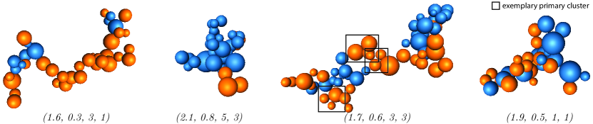
Figure 2: Examples of virtual hetero-aggregates. The labels correspond to the values of the vector $\theta=(\theta_{\mathrm{D_{f}}},\theta_{\mathrm{\uprho}},\theta_{\mathrm{0}},\theta_{\mathrm{1}})$ of their model parameters. The WO3 particles are displayed in blue, while the TiO2 particles are displayed in orange. The particle sizes are drawn from a log-normal distribution with parameters $\mu$ and $\sigma$ as defined above. Some primary clusters, as defined in Section 2.1.1, are highlighted.

2.1.3 Simulation of STEM intensities

After generating virtual hetero-aggregates, reference simulations to calculate the high-angle annular darkfield (HAADF)-STEM intensity of TiO2 and WO3 are conducted as a function of the sample thickness and material density. For that purpose, multi-slice simulations in the frozen-lattice approach [41] with the STEMSIM software [35] were performed. Simulations were done for the rutile and anatase phases of TiO2 as well as for gamma and delta phases of WO3. Crystal parameters and Debye-Waller factors were taken from [5, 14, 24, 38], and elastic atomic scattering amplitudes from [21] were used. The HAADF-STEM intensity for microscope parameters equal to those one would use in experiments with a ThermoFisher 60/300 Spectra microscope were simulated. This machine is equipped with a Cs-corrector for the probe forming system, an X-FEG and SuperXG2 EDXS detectors. A semi-convergence angle of $\beta=21.1\,\mathrm{mrad}$ and an acceleration voltage of $300\,\mathrm{kV}$ were set. The simulated HAADF-STEM intensity was obtained by integration of electrons scattered into the annular range between $55\,\mathrm{mrad}$ and $250\,\mathrm{mrad}$ after application of a detector specific sensitivity curve [35].

The HAADF-STEM intensity further depends on the orientation of the crystal with respect to the electron beam. To account for this effect, various orientations for each material and phase of the crystal were simulated.

Therefore, the crystal was systematically tilted in nine equal steps from a [100]- towards a [010]-viewing direction. In addition, a random tilt was simulated. The final result is a data set with the HAADF-STEM intensity as a function of the sample thickness for TiO2 and WO3, each in two different crystal phases, each with ten orientations of the crystal with respect to the electron beam.

2.1.4 Generation of realistic STEM images

The third step combines the HAADF-STEM reference simulations described above with the virtual 3D hetero-aggregates. STEM images show 2D projections of the aggregates, see Figure 3. Therefore, the projections of the individual particles along one direction are computed, as usual in electron microscopy, the electron beam direction and hence the projection direction is referred to as $z$-direction. This results in thickness maps for the individual particles. Using the reference simulations, these thickness maps are translated into maps of the HAADF-STEM intensities. To this end, for each particle, the reference simulation of the respective material was chosen in a random phase and a random orientation of the crystal with respect to the electron beam.

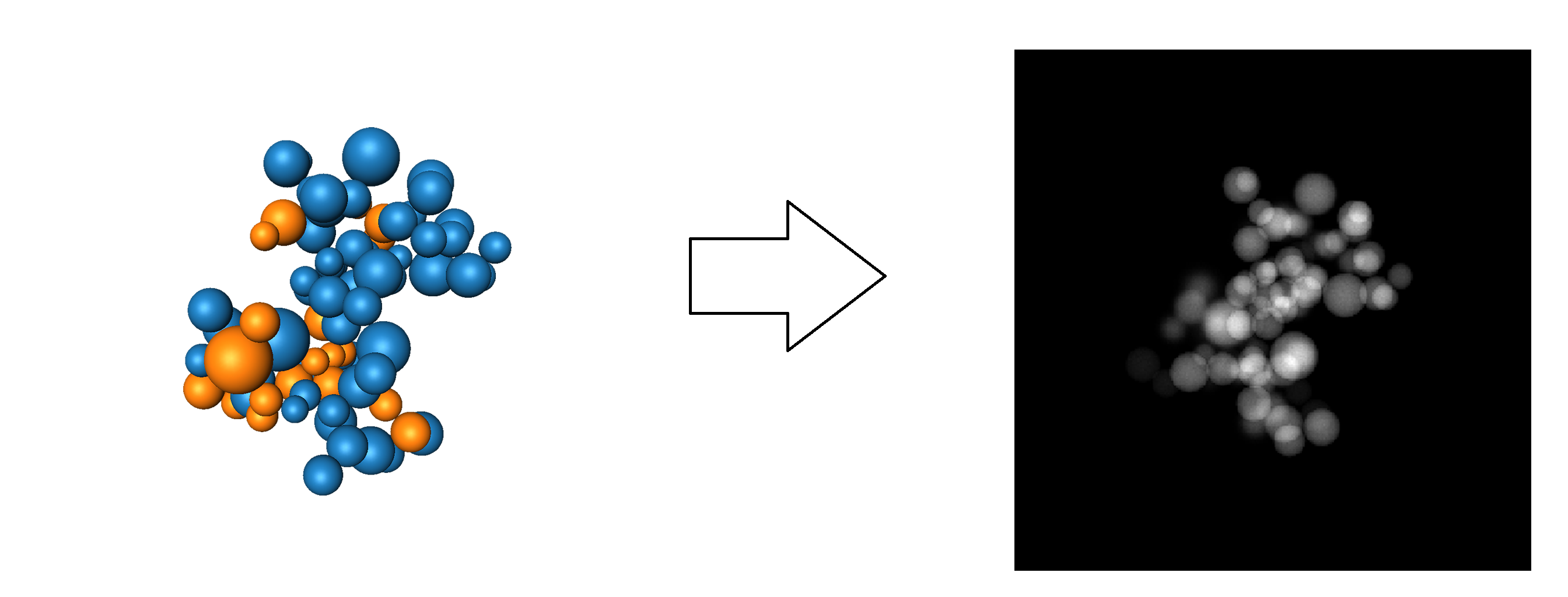
Figure 3: Schematic representation of the 3D structure of a virtual hetero-aggregate (left) and its respective STEM image (right). The WO3 particles are colored blue and correspond to the bright particles in the STEM image. The TiO2 particles are colored orange and correspond to the dark particles.

In an aggregate, which extends several tens of nanometers in $z$-direction, not all particles appear in focus. Only particles with centers located at height $z=0\,\mathrm{nm}$ are in focus as the electron beam is focused on this plane. To account for this effect, each HAADF-STEM map of the individual particles is convolved with a Gaussian kernel. More precisely, for a particle located at height $z$, the standard deviation $\sigma_{\mathrm{STEM}}$ of the Gaussian kernel with which the corresponding HAADF-STEM map is convoluted is chosen as $\sigma_{\mathrm{STEM}}=|z|\cdot\tan(\beta)$, where $\beta=21.1\,\mathrm{mrad}$ is the semi-convergence angle, assuming a conical beam shape. Then, blurred HAADF-STEM maps of individual particles are summed up to obtain the artificial HAADF-STEM image of the hetero-aggregate. Finally, shot noise according to a typical electron dose of $149\,\mathrm{electrons/\text{\AA}^{2}}$ [23] and scan noise according to a possible typical beam displacement of $0.01\,\mathrm{nm}$ [17] were applied.

2.2 Statistical analysis and processing of simulated data

In this section the need for the usage of neural networks is explained, addressing some problems connected with the reconstruction of preset values of the model parameters $\theta_{\mathrm{D_{f}}},\theta_{\mathrm{\uprho}},\theta_{\mathrm{0}},\theta_{\mathrm{1}}$, based on virtual aggregates drawn from the stochastic 3D model. Further complications in this reconstruction task arise when using 2D STEM data instead of the full 3D geometry of the aggregates, through a loss of information. Therefore, it is explained how image processing methods can be used to simplify the extraction of information from STEM data.

2.2.1 Estimating the parameters of the stochastic 3D model

One of the challenges associated with predicting the parameters of the stochastic 3D model from STEM images is that some model parameters are even imperceivable from the 3D structure of a virtual aggregate from which the corresponding STEM image is determined. This is due to the simplifying assumptions made within the simulation process of the 3D model and its stochastic nature, see Section 2.1.2, resulting in empirical values of the model parameters slightly differing from the preset ones.

For example, the fractal dimension $D_{\mathrm{f}}$ computed by means of Eq. (5) for a virtual hetero-aggregate $A$ might differ from the preset value of the model parameter $\theta_{\mathrm{D_{f}}}$. More precisely, in the simulation of hetero-aggregates, the radii $r_{1},\ldots,r_{N}$ of particles considered in Eq. (5) are replaced by their arithmetic mean $(r_{1}+\ldots+r_{N})/N$, see Section 2.1.2. Also, the mixing ratio $\rho$ of an aggregate $A$ computed by means of Eq. (3) can deviate from the model parameter $\theta_{\mathrm{\uprho}}$, due to the randomly chosen labels of primary clusters, modeled by the Bernoulli-distributed random variables $L_{1},\ldots,L_{N^{\prime}}$. For example, the first aggregate in Figure 2 has an expected (preset) mixing ratio of $\theta_{\mathrm{\uprho}}=0.3$, but the actual mixing ratio $\rho$ computed from Eq. (3) is $\rho=\frac{9}{41}\approx 0.22$. Recall that, in order to distinguish between these quantities, the vector of model parameters used to generate $A$ is referred to as $\theta=({\theta_{\mathrm{D_{f}}}},{\theta_{\mathrm{\uprho}}},{\theta_{\mathrm{0}}},{\theta_{\mathrm{1}}})$, while $D_{\mathrm{f}}(A)$ and $\rho(A)$ describe the empirical fractal dimension and mixing ratio of the aggregate $A$, computed from Eqs. (5) and (3), respectively.

Figure 4 illustrates the discrepancy between preset model parameters and the empirical fractal dimension and mixing ratio of virtual aggregates, computed from Eqs. (5) and (3), respectively. Nevertheless, Figure 4 indicates that, on average, the structural descriptors $D_{\mathrm{f}}$ and $\rho$ nicely coincide with the preset model parameters $\theta_{\mathrm{D_{f}}}$ and $\theta_{\mathrm{\uprho}}$. Therefore, rather than attempting to determine the model parameters ${\theta_{\mathrm{D_{f}}}},{\theta_{\mathrm{\uprho}}},{\theta_{\mathrm{0}}},{\theta_{\mathrm{1}}}$ from a single aggregate $A$, a family $B=\{A_{1},\ldots,A_{\nu}\}$ of $\nu>1$ aggregates is used instead, called batch in the following. More specifically, it is expected that choosing a larger batch size would yield more accurate results, but at an increased cost.

Figure 4: Visualization of empirical probability densities of the fractal dimension $D_{\mathrm{f}}(A)$ (left) and mixing ratio $\rho(A)$ (right) of virtual hetero-aggregates, depending on the model parameters $\theta_{\mathrm{D_{f}}}$ and $\theta_{\mathrm{\uprho}}$, where the values of $D_{\mathrm{f}}(A)$ and $\rho(A)$ are computed by means of Eqs. (5) and (3), respectively. The other model parameters were chosen at random from their respective ranges, as introduced in Section 2.1.2. To improve clarity, kernel density estimation was used to assign colors to the scatter points computed for $19\,440$ realizations of the stochastic 3D model.

We were not able to find any scalar features that can be utilized to predict the model parameters $\theta_{\mathrm{0}}$ and $\theta_{\mathrm{1}}$ associated with the cluster size used in the generation of virtual aggregates, i.e., in the cluster-cluster-model introduced in Section 2.1.1. For example, in order to predict the model parameter $\theta_{\mathrm{0}}$, an obvious choice for such a scalar feature would be to describe the average size of observable WO3 clusters, where an observable cluster is an inclusion maximal homogeneous subset $C\subset A$ of an aggregate $A$, i.e., there is no larger homogeneous subset $C^{\prime}\subset A$ such that $C\subset C^{\prime}$. These clusters can differ from the primary clusters used in the construction algorithm described in Section 2.1.1. Specifically, the observable clusters are formed by unions of primary clusters, whereas, contrary to the latter ones, the observable clusters are recognizable in the 3D data, see Figure 2 for a visualization.

However, this average (observable) cluster size can not be used to predict $\theta_{\mathrm{0}}$. Figure 5 shows that there are various specifications of model parameters that differ in $\theta_{\mathrm{0}}$ and, nevertheless, yield similar average cluster sizes of WO3 particles.

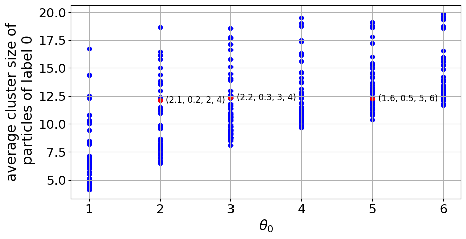
Figure 5: Average cluster size of WO3 particles. Each scatter point is computed over a batch $B=\{A_{1},\ldots,A_{\nu}\}$ with $\nu=12$ for six different specifications of the model parameters $\theta_{\mathrm{D_{f}}},\theta_{\mathrm{\uprho}},\theta_{\mathrm{0}},\theta_{\mathrm{1}}$. For three of these specifications, the values of $\theta=(\theta_{\mathrm{D_{f}}},\theta_{\mathrm{\uprho}},\theta_{\mathrm{0}},\theta_{\mathrm{1}})$ and the average cluster sizes, corresponding to the red scatter points, are displayed.

The prediction of the model parameter vector $\theta$ is further complicated by the fact that only the 2D STEM image can be utilized which may not perfectly inform the 3D morphology of $A$.

To predict the preset vector of model parameters $\theta$ from a family $B$ of aggregates using only their simulated STEM images, CNNs are initially utilized to extract relevant features from these images. These features are subsequently utilized to predict the preset model parameters, see the schematic description of this workflow shown in Figure 1b. While the process of extracting features from the STEM images remains largely consistent across all model parameters, the calculation of the estimators for ${\theta_{\mathrm{D_{f}}}},{\theta_{\mathrm{\uprho}}},{\theta_{\mathrm{0}}},{\theta_{\mathrm{1}}}$ exhibits significant variations, see Sections 2.3.2-2.3.5 below. For instance, when estimating the model parameters $\theta_{\mathrm{D_{f}}}$ and $\theta_{\mathrm{\uprho}}$, the features computed from a STEM image $I$ of an aggregate $A$ are scalar values that approximate $D_{\mathrm{f}}(A)$ and $\rho(A)$. Then, the arithmetic mean of the respective image-wise features of a family $B=\{A_{1},\ldots,A_{\nu}\}$ of aggregates is used as estimators $\widehat{\theta}_{\mathrm{D_{f}}}$ and $\widehat{\theta}_{\mathrm{\uprho}}$ for $\theta_{\mathrm{D_{f}}}$ and $\theta_{\mathrm{\uprho}}$. In contrast, when predicting the model parameters $\theta_{\mathrm{0}}$ and $\theta_{\mathrm{1}}$, a neural network is employed to identify high-dimensional features from which the estimators $\widehat{\theta}_{\mathrm{0}}$ and $\widehat{\theta}_{\mathrm{1}}$ for $\theta_{\mathrm{0}}$ and $\theta_{\mathrm{1}}$ are computed, see Section 2.3 below.

2.2.2 Data processing and augmentation

Various common image processing methods are used to simplify the extraction of information from STEM images. In particular, the pixel intensity values of STEM images are linearly scaled to the entire range of $[-0.5,0.5]$ and rounded to $256$ equidistant values in order to achieve faster convergence to a lower error during the training process. More specifically, the scaling centers the pixel intensity values around zero [32], whereas the rounding reduces the noise of the images. Note that this procedure is performed on all STEM images, even if not explicitly mentioned, whereas the subsequent preprocessing steps will only be applied during training.

Overfitting is a common problem where neural networks achieve good results on training data but perform rather poorly when applied to previously unseen data. This can occur when the model learns irrelevant information within the dataset. As a result, the model fits too closely to the training set and becomes overfitted, making it unable to generalize well to new data. To address this issue, augmentation of training data is used. In the context of the present paper, this means that the input data is randomly modified in each training step, such that during each step of the training procedure the network is provided with input data which differs from the input data of previous steps. Therefore, a significantly larger number of training steps can be conducted while still providing the neural network with novel training data in each step, and thus, avoiding overfitting.

Note that there is a wide variety of possible methods for modifying input data which are commonly used in training data augmentation, e.g., rotation, reflection, radial transformation, elastic distortion [37] and random erasing [36]. However, in order to preserve certain structural descriptors of aggregates observed in image data, like shape and size descriptors of particles, only random rotations, reflections and small displacements are used for training data augmentation.

2.3 CNN-based approach for the prediction of model parameters

The goal of this section is to introduce the CNN-based methodology for predicting the model parameters $\theta_{\mathrm{D_{f}}},\theta_{\mathrm{\uprho}},\theta_{\mathrm{0}},\theta_{\mathrm{1}}$ of the hetero-aggregate model from (simulated) STEM images.

Due to computational constraints, it was not feasible to generate the required number of aggregates for each possible preset of the model parameters $\theta_{\mathrm{D_{f}}},\theta_{\mathrm{\uprho}},\theta_{\mathrm{0}},\theta_{\mathrm{1}}$. Therefore, in order to ensure robust training, the focused was on generating 100 aggregates for each triple $(\theta_{\mathrm{\uprho}},\theta_{\mathrm{0}},\theta_{\mathrm{1}})$ in $\{0.1,\ldots,0.9\}\times\{1,\ldots,6\}\times\{1,\ldots,6\}$, as these parameters exhibited interactive effects that were crucial for our study. More specifically, for each such triple, two values $\theta_{\mathrm{D_{f}}}^{(1)},\theta_{\mathrm{D_{f}}}^{(2)}$ of $\theta_{\mathrm{D_{f}}}$ were chosen at random from $\{1.5,\ldots,2.5\}$ and each resulting model parameter preset $(\theta_{\mathrm{D_{f}}}^{(1)},\theta_{\mathrm{\uprho}},\theta_{\mathrm{0}},\theta_{\mathrm{1}}),(\theta_{\mathrm{D_{f}}}^{(2)},\theta_{\mathrm{\uprho}},\theta_{\mathrm{0}},\theta_{\mathrm{1}})$ was used to generate 50 aggregates. After applying the STEM simulation described in Section 2.1, this results in a set $G=\{(A_{i},I_{i},\theta_{i}):1\leq i\leq 32\,400\}$ of 32 400 triplets of 3D aggregates $A_{i}$, corresponding STEM images $I_{i}$, and vectors of preset model parameters $\theta_{i}=({\theta_{\mathrm{D_{f}}}}_{,i},{\theta_{\mathrm{\uprho}}}_{,i},{\theta_{\mathrm{0}}}_{,i},{\theta_{\mathrm{1}}}_{,i})$. The set $G$ is thereafter split into two datasets, one for training and one for evaluation.

For both, training and evaluation, batches

$$B=\{(A_{i_{1}},I_{i_{1}},\theta_{i_{1}}),\ldots,(A_{i_{v}},I_{i_{v}},\theta_{i_{v}})\}\subset G$$ (9)

will be used for some $\nu>1$, that are generated by the same preset of model parameters, i.e., $\theta_{i_{1}}=\ldots=\theta_{i_{v}}$. To ensure the availability of such batches, the split of $G$ is done such that there is no model parameter configuration that occurs less than 20 times in neither the data used for training nor in the data used for evaluation. These two datasets will be referred to by their respective index sets $T$ (for training) and $E$ (for evaluation), where $T\cup E=\{1,\dots,32\,400\}$ with $\#T=19\,440$ and $\#E=12\,960$.

In the following, it is explained how the triplets $(A_{i},I_{i},\theta_{i})$ are used to generate pairs of image data and ground truth labels, which will be utilized for the training of the neural networks. First, general aspects of network architecture and training are presented and, then, some specifics regarding the prediction of each of the four model parameters ${\theta_{\mathrm{D_{f}}}},{\theta_{\mathrm{\uprho}}},{\theta_{\mathrm{0}}},{\theta_{\mathrm{1}}}$ are given.

2.3.1 Network architecture and training

The networks used to extract features are all based on the same basic network architecture, regardless of the model parameter being predicted. This network architecture consists of stacked convolutional layers with a kernel size of $3\times 3$, batch normalization layers [15], the ReLu activation function, given by

$$\text{ReLu}(x)=\max\{0,x\}\qquad\mbox{for $x\in\mathbb{R}$,}$$ (10)

and max pooling layers with a kernel size of $2\times 2$, followed by fully connected layers. The basic architecture of the convolutional neural networks considered in the following has the form

$$CNN=g(f)\,,$$ (11)

i.e., it is represented as the composition of two subnetworks, $f$ and $g$. The subnetwork $f$ consists of the convolutional part of the basic network architecture, a flatten layer and two dense layers with a final output dimension of 112. The subnetwork $g$ consists of two dense layers with a final output dimension of 1. A schematic representation of the network architecture is given in Figure 6 (left), whereas details regarding the this architecture are provided in Table 3.

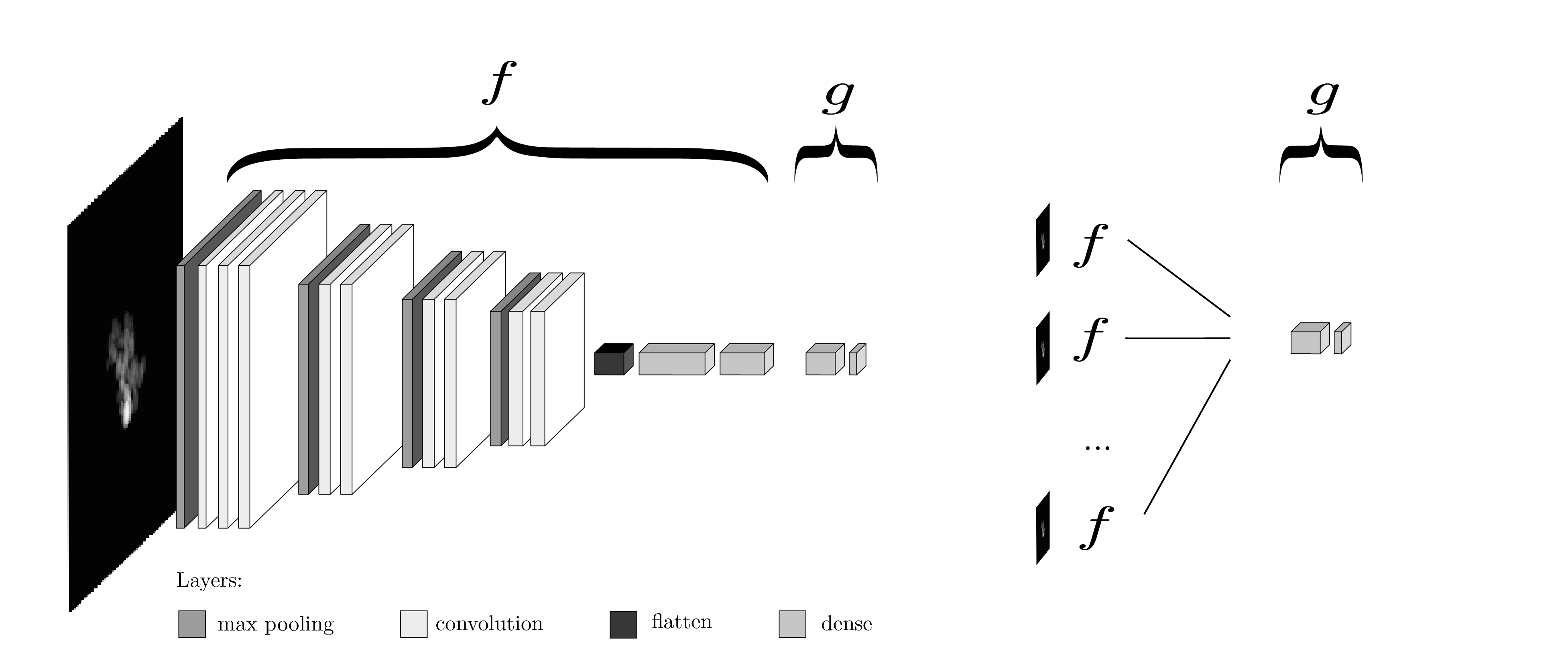
Figure 6: The basic network architecture represented as a simple composition of subnetworks $f$ and $g$ (left), and an adjusted multi-image input network (right), where the subnetwork $f$ is applied to multiple input images and the outputs are concatenated as a new input for subnetwork $g$ (see also Section 2.3.4 below).

	layer	output shape	number of parameters
0	input	$(512,512,1)\cdot b$	$0\cdot 1$
1	average pooling	$(256,256,1)\cdot b$	$0\cdot 1$
2	convolution + batch norm. + ReLu	$(254,254,8)\cdot b$	$(80+56+0)\cdot 1$
3	convolution + batch norm. + ReLu	$(252,252,16)\cdot b$	$(1\,168+112+0)\cdot 1$
4	convolution + batch norm. + ReLu	$(250,250,32)\cdot b$	$(4\,640+224+0)\cdot 1$
5	max pooling	$(125,125,32)\cdot b$	$0\cdot 1$
6	convolution + batch norm. + ReLu	$(123,123,64)\cdot b$	$(18\,496+448+0)\cdot 1$
7	convolution + batch norm. + ReLu	$(121,121,64)\cdot b$	$(36\,928+448+0)\cdot 1$
8	max pooling	$(60,60,64)\cdot b$	$0\cdot 1$
9	convolution + batch norm. + ReLu	$(58,58,128)\cdot b$	$(73\,856+896+0)\cdot 1$
10	convolution + batch norm. + ReLu	$(56,56,128)\cdot b$	$(147\,584+896+0)\cdot 1$
11	max pooling	$(28,28,128)\cdot b$	$0\cdot 1$
12	convolution + batch norm. + ReLu	$(26,26,256)\cdot b$	$(295\,168+1\,792+0)\cdot 1$
13	convolution + batch norm. + ReLu	$(24,24,256)\cdot b$	$(590\,080+1\,792+0)\cdot 1$
14	max pooling	$(12,12,256)\cdot b$	$0\cdot 1$
15	flatten	$(36\,864)\cdot b$	$0\cdot 1$
16	dense + ReLu	$(224)\cdot b$	$8\,257\,760\cdot 1$
17	dense + ReLu	$(112)\cdot b$	$25\,200\cdot 1$
18	dense + ReLu	$(44)$	$112\cdot b\cdot 44+44$
19	dense	$1$	$45\cdot 1$
			$=b\cdot 4\,928+9\,457\,713$

Table 3: Details of network architecture. The value of $b$ is put equal to $b=1$ for the prediction of the model parameters $\theta_{\mathrm{D_{f}}}$ and $\theta_{\mathrm{\uprho}}$, and $b=\nu$ for the prediction of $\theta_{\mathrm{1}}$ and $\theta_{\mathrm{0}}$. Since padding is omitted, each convolutional layer reduces the size of the feature map by two in both dimensions.

To achieve a high prediction quality, the parameters of the neural networks have to be adopted. This will be done supervised. More precisely, the dissimilarity between the ground truth, denoted as $y=(y_{1},\ldots,y_{n})$, and the network output $\widehat{y}=(\widehat{y}_{1},\ldots,\widehat{y}_{n})$, i.e., $\widehat{y}_{1}=\mathrm{CNN}(x_{1}),\ldots,\widehat{y}_{n}=\mathrm{CNN}(x_{n})$ for some input $x=(x_{1},\ldots x_{n})$, $n>1$, will be minimized. For example, when predicting the fractal dimension $\theta_{\mathrm{D_{f}}}$, the input $x$ of the network consists of STEM images $I_{1},...,I_{n}$ and the ground truth is given by the vector of fractal dimensions of the respective aggregates $A_{1},...,A_{n}$, i.e. $y=(D_{\mathrm{f}}(A_{1}),...,D_{\mathrm{f}}(A_{n}))$. The comparison between the ground truth and the prediction is done in terms of the mean square error (MSE), given by

$$\mathrm{MSE}(y,\widehat{y})=\frac{1}{n}\sum_{i=1}^{n}(y_{i}-\widehat{y}_{i})^{2}.$$ (12)

The resulting loss $\mathrm{MSE}(y,\widehat{y})$ is minimized by a gradient descent method using an Adam optimizer [13, 20] with a learning rate of $0.0001$, where the value of $n$ in Eq. (12) determines the number of network evaluations before a step of the gradient descent method is applied. These evaluations are done on the training data, given by the index set $T$, where $n$ is put to $16$ when predicting $\theta_{\mathrm{D_{f}}}$ or $\theta_{\mathrm{\uprho}}$, and $n=8$ otherwise.

The general network architecture described above and the prediction procedure will be slightly adapted for each of the four model parameters $\theta_{\mathrm{D_{f}}},\theta_{\mathrm{\uprho}},\theta_{\mathrm{0}}$ and $\theta_{\mathrm{1}}$. In the following, detailed explanations will be provided regarding these parameter-specific adaptations.

2.3.2 Fractal dimension

The fractal dimensions $D_{\mathrm{f}}(A_{i_{1}}),\ldots,D_{\mathrm{f}}(A_{i_{\nu}})$ of the aggregates $A_{i_{1}},\ldots,A_{i_{\nu}}$ in a batch $B$, as introduced in Eq. (9), are typically symmetrically distributed around the preset value of $\theta_{\mathrm{D_{f}}}$, which will be denoted by $\theta_{\mathrm{D_{f}}}(B)$ in the following, see Figure 4a. Therefore, the mean value $\overline{D}_{\mathrm{f}}(B)$, given by

$$\overline{D}_{\mathrm{f}}(B)=\frac{1}{\nu}\sum_{k=1}^{\nu}D_{\mathrm{f}}(A_{i_{k}}),$$

could be used as an estimator for $\theta_{\mathrm{D_{f}}}(B)$. However, since the fractal dimensions $D_{\mathrm{f}}(A_{i_{1}}),\ldots,D_{\mathrm{f}}(A_{i_{\nu}})$ cannot be directly determined from the STEM images $I_{i_{1}},\ldots,I_{i_{\nu}}$, approximations $\widehat{D}_{\mathrm{f}}(I_{i_{1}}),\ldots,\widehat{D}_{\mathrm{f}}(I_{i_{\nu}})$ are used instead. These approximations are computed by a convolutional neural network $\mathrm{CNN^{\mathrm{D_{f}}}}$, where the STEM images $I_{i_{1}},\ldots,I_{i_{\nu}}$ are used as input. Thus, finally, the estimator $\widehat{\theta}_{\mathrm{D_{f}}}(B)$ for $\theta_{\mathrm{D_{f}}}(B)$ is given by

$$\widehat{\theta}_{\mathrm{D_{f}}}(B)=\frac{1}{\nu}\sum_{j=1}^{\nu}\widehat{D}_{\mathrm{f}}(I_{i_{j}})=\frac{1}{\nu}\sum_{j=1}^{\nu}\mathrm{CNN^{\mathrm{D_{f}}}}(I_{i_{j}}).$$ (13)

The architecture of the neural network $\mathrm{CNN^{\mathrm{D_{f}}}}$ coincides with the one described in Section 2.3.1. The activation function of the output layer is a scaled sigmoid function. This kind of activation function is a standard choice for NNs with bounded outputs. More precisely, the activation function is given by $\gamma(x)=\alpha\frac{1}{1+e^{-x}}+\beta$ for $x\in\mathbb{R}$, where $\alpha=1.4$ and $\beta=1.3$ are selected to ensure that the network can represent the expected range of values for $D_{\mathrm{f}}$, with added tolerances on each side of the expected range, see Figure 4a. Note that the input of the network during training consists of augmented versions $a(I_{i})$ of the STEM images $I_{i}$ for $i\in T$, i.e., images that arise from $I_{i}$ by reflecting, rotating and displacing, as described in Section 2.2.2. The corresponding supervisory signal consists of the fractal dimension of the corresponding aggregates. Hence, the network training is conducted using pairs $(a(I_{i}),D_{\mathrm{f}}(A_{i}))$, for $i\in T$.

2.3.3 Mixing ratio

In Figure 4b the distribution of the mixing ratio of aggregates in dependence of the model parameter $\theta_{\mathrm{\uprho}}$ is visualized. From there, it is evident that the mixing ratios $\rho(A_{i_{1}}),\ldots,\rho(A_{i_{\nu}})$ of aggregates $A_{i_{1}},\ldots,A_{i_{\nu}}$ within a batch $B$, generated by the 3D model with a preset value of $\theta_{\mathrm{\uprho}}(B)$, follow a distribution the mean of which is approximately equal to $\theta_{\mathrm{\uprho}}(B)$.

This suggests using a similar approach as described above in Section 2.3.2. However, note that there are some aggregates with a mixing ratio $\rho(A_{i})$ being equal to $0$ or $1$. A neural network with an architecture as that of $\mathrm{CNN^{\mathrm{D_{f}}}}$ does not reflect these discrete values properly. Therefore, the prediction procedure for the mixing ratio is slightly modified by initially classifying whether an image $I_{i}$ depicts an aggregate with mixing ratio of exactly $0$ or $1$, using a classification network $\mathrm{CNN_{class}^{\rho}}$, and afterwards predicting the mixing ratio of the corresponding aggregate, using a regression network $\mathrm{CNN_{reg}^{\rho}}$. For this purpose, the networks $\mathrm{CNN_{class}^{\rho}}$ and $\mathrm{CNN_{reg}^{\rho}}$, having the same basic network architecture as described in Section 2.3.1 and a commonly used [39] unscaled sigmoid function $\gamma(x)=\frac{1}{1+e^{-x}}$ for $x\in\mathbb{R}$ as activation function in the output layer, are trained for the respective tasks. The training of the regression network $\mathrm{CNN_{reg}^{\rho}}$ is done on pairs $(a(I_{i}),\rho(A_{i}))$, $i\in T$, of augmented STEM images and corresponding ground truth mixing ratios, whereas the training of the classification network $\mathrm{CNN_{class}^{\rho}}$ is done on pairs of augmented STEM images and corresponding binary class labels, where a class label of $0$ or $1$ identifies the corresponding aggregate as heterogeneous or homogeneous, respectively.

However, it is a well-known problem that number-wise imbalanced classes can lead to poorly performing classifications since classifiers tend to neglect the underrepresented classes, also known as imbalance problem [29]. To address this issue, the augmented STEM images of homogeneous aggregates, which account for about 10% of all images, were oversampled in the training procedure of the classifier to achieve balanced classes.

Finally, to predict the mixing ratio of an aggregate via its STEM image, the outputs of $\mathrm{CNN_{class}^{\rho}}$, which identifies homogenous aggregates, and $\mathrm{CNN_{reg}^{\rho}}$, which determines the mixing ratio, are combined. More specifically, for a STEM image $I$, the predicted mixing ratio $\widehat{\rho}(I)$ of the corresponding aggregate is given by

$$\widehat{\rho}(I)=\begin{cases}\eta\left(\mathrm{CNN_{reg}^{\rho}}(I)\right),&\text{if }\mathrm{CNN_{class}^{\rho}}(I)>0.5,\\ \mathrm{CNN_{reg}^{\rho}}(I),&\text{else,}\end{cases}$$

where $\eta:[0,1]\rightarrow\{0,1\}$ is the function that rounds a number $x\in[0,1]$ to its closest integer $\eta(x)\in\{0,1\}$. This results in the estimator $\widehat{\theta}_{\mathrm{\uprho}}(B)$ for the preset model parameter $\theta_{\mathrm{\uprho}}(B)$ of a batch $B=\{(A_{i_{1}},I_{i_{1}},\theta_{i_{1}}),\ldots,(A_{i_{v}},I_{i_{v}},\theta_{i_{v}})\}$, given by

$$\widehat{\theta}_{\mathrm{\uprho}}(B)=\frac{1}{\nu}\sum_{j=1}^{\nu}\widehat{\rho}(I_{i_{j}}).$$ (14)

2.3.4 Size of primary WO3 clusters

In the procedures for predicting the model parameters $\theta_{\mathrm{D_{f}}}$ and $\theta_{\mathrm{\uprho}}$, described above, the process of determining an estimator involved the identification of a scalar feature that describes an aggregate property, namely, the fractal dimension $D_{\mathrm{f}}$ and the mixing ratio $\rho$, that is predominantly influenced by the corresponding model parameter. This scalar feature can be directly computed from the virtual 3D aggregates, and thus, it is possible to predict it from the corresponding 2D STEM images. Consequently, using this scalar feature, formulas for estimating the model parameter from this property has been derived, see Eqs. (13) and (14).

Since the model parameter $\theta_{\mathrm{0}}$ is designed to control the cluster sizes of WO3 particles for the cluster-cluster-aggregation model introduced in Section 2.1.1, such a property should relate to the number of connected WO3 particles. However, the sizes of observable clusters are not only influenced by $\theta_{\mathrm{0}}$ but also by $\theta_{\mathrm{\uprho}}$. On the one hand, larger values of $\theta_{\mathrm{0}}$ lead to larger primary cluster sizes of clusters of label 0 and thus larger observable clusters. Lower values of $\theta_{\mathrm{\uprho}}$ lead to larger proportions of primary clusters of label 0. Therefore, it is more likely that two primary clusters that are in contact, share the material label 0, and thus, the expected size of observable clusters of label 0 increases, see Figure 5.

This makes the average of the observable cluster size on its own an unsuitable property for estimating the model parameter $\theta_{\mathrm{0}}$. Therefore, one has to search for another feature that is functionally related to $\theta_{\mathrm{0}}$. Additionally, a functional relationship that suitably maps features derived from STEM images to an estimator of $\theta_{\mathrm{0}}$ may not be captured solely by an average, necessitating the search for another suitable function. However, these two steps can be quite complex and time-consuming if done heuristically. To address this, a data-driven approach utilizing a neural network is adopted. This approach allows us to determine the feature vectors and the formula that relates them to the corresponding model parameter $\theta_{\mathrm{0}}$. More specifically, the identification of relevant features is conducted by means of part $f$ of the basic network architecture described in Section 2.3.1. The subnetwork $f$ is applied to all images in a batch individually, and the concatenated results are then used as input of part $g$ of the basic network architecture, which is in charge of determining the relationship between the feature vectors determined by $f$ and the model parameter $\theta_{\mathrm{0}}$. In detail, this results in a modified network, denoted as CNN⁰, which is given by

$${\rm CNN}^{0}(I(B))=g(f(I_{i_{1}}),\ldots,f(I_{i_{\nu}})),$$ (15)

where $I(B)=\{I_{i_{1}},\ldots,I_{i_{\nu}}\}$ denotes the STEM images corresponding to the aggregates $A_{i_{1}},\ldots,A_{i_{\nu}}$ in a batch $B$. Referring to Table 3, the feature vectors of STEM images up to the output of layer 17 are computed as before. Then these feature vectors of a batch are concatenated and used as input of layer 18. The final output layer uses a ReLu transfer function. The modified network architecture is illustrated on the right-hand side of Figure 6.

Note that the approach described above differs from the commonly used technique where a network, denoted as $f^{\prime}$, takes multi-channel input data, i.e., in our case $f^{\prime}(I_{i_{1}},...,I_{i_{\nu}})$. Such an approach allows the network to detect spatially resolved interdependencies among the images. In contrast, our approach considered in Eq. 15 employs identical CNNs $f$ for dimensionality reduction and feature extraction on each input channel individually. As a consequence, this ensures uniform feature extraction for every input image while also reducing the number of trainable parameters in the CNN. The choice of this approach is rooted in the concept that each image within a batch a priori contains the same information regarding the underlying model parameters, and the lack of spatial interdependence between the images which would be relevant for the prediction of model parameters.

Due to the problem-specific architecture of the network $\mathrm{CNN^{0}}$, the training data no longer consists of pairs of individual images and corresponding ground truths. Instead, for each batch $B$, the training pair $(\{a(I_{i_{1}}),\ldots,a(I_{i_{\nu}})\},\theta_{\mathrm{0}}(B))$ consists of a corresponding batch of augmented images and the underlying model parameter $\theta_{\mathrm{0}}(B)$.

Since the model parameter $\theta_{\mathrm{0}}$ can only take integer values, the output of the network has to be rounded to obtain a valid estimator for $\theta_{\mathrm{0}}$, given by $\widehat{\theta}_{\mathrm{0}}(B)=\eta(\mathrm{CNN^{0}}(I(B))$, where where $\eta:[0,\infty)\rightarrow\{0,1,\ldots\}$ is the function that rounds a number $x\geq 0$ to its closest integer $\eta(x)\in\{0,1,\ldots\}$.

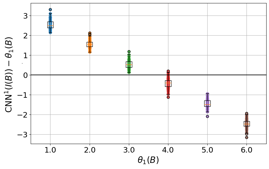
Figure 7: Prediction error of the network $\mathrm{CNN^{1}}$ for unmodified input images, in dependence of the preset value of the model parameter $\theta_{\mathrm{1}}$. The prediction quality is comparable to that of a constant prediction, where $\mathrm{CNN^{1}}(I(B))=3.5$. The results have been obtained on a randomly chosen subset of the training data set.

2.3.5 Size of primary TiO2 clusters

The method used to predict the model parameter $\theta_{\mathrm{1}}$ for the cluster size of TiO2 particles is similar to the approach described in the previous section. Nonetheless, given that the pixel intensity values of TiO2 particles in the STEM images closely resemble the background and are significantly lower than those of WO3 particles, they are considerably more difficult to differentiate by visual inspection. Consequently, it might be plausible that a neural network could also encounter challenges in tasks which depend on the identification of TiO2 particles. As shown in Figure 7, the neural network $\mathrm{CNN^{1}}$ achieves unsatisfactory results when using unadjusted image data, which may be due to the difficulty mentioned above.

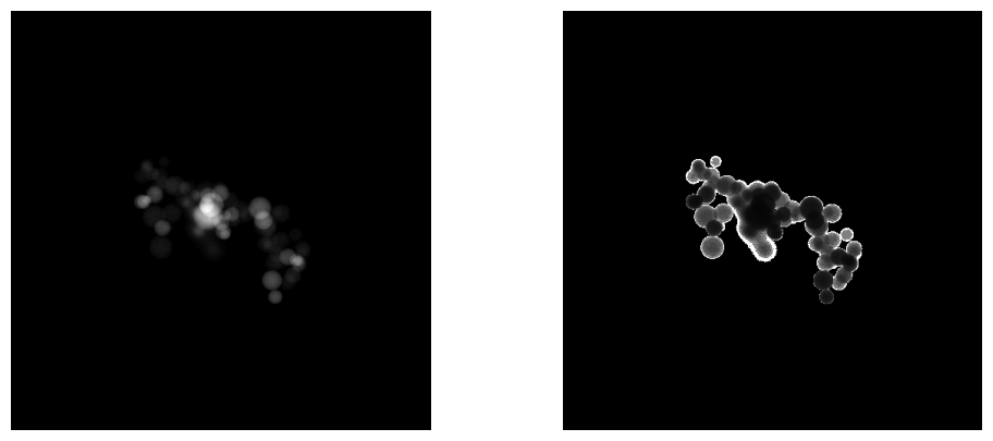
Figure 8: Effect of pixel intensity modification. The image on the right-hand side is obtained after replacing the intensity values of non-background pixels (shown on the left-hand side) by their multiplicative inverse, where a treshhold of $t=0.001$ is used.

To address this issue, the intensity value $p>0$ of non-background pixels in the STEM images is replaced by its multiplicative inverse $p^{\mathrm{modified}}$, i.e., for some threshold $t>0$ the modified pixel value is given by

$$p^{\mathrm{modified}}=\begin{cases}p,&\quad\mbox{if $0<p<t$,}\\ \displaystyle p^{-1},&\quad\text{otherwise.}\end{cases}$$

This procedure is applied to all STEM images used in the prediction of $\theta_{\mathrm{1}}$ before the preprocessing steps described in Section 2.2.2 are applied. The highlighting effect of this adjustmemt of pixel intensity values is shown in Figure 8.

3 Results

In this section, the results of the analysis on various aspects of model parameter prediction are presented. To ensure that these results accurately represent the generalization capability of the trained neural networks, all evaluations were conducted on data not used during training. More specifically, recall that the data corresponding to the index set $T$ is used for training, whereas the data corresponding to the index set $E$ is used to evaluate results, see Section 2.3 for details on the training-test split.

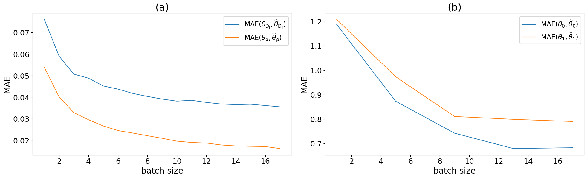
Figure 9: Quality of the estimators for ${\theta_{\mathrm{D_{f}}}},{\theta_{\mathrm{\uprho}}},{\theta_{\mathrm{0}}},{\theta_{\mathrm{1}}}$, in dependence of the batch size $\nu$. Due to different orders of magnitude, the error curves for ${\theta_{\mathrm{D_{f}}}},{\theta_{\mathrm{\uprho}}}$ and ${\theta_{\mathrm{0}}},{\theta_{\mathrm{1}}}$ are shown separately. The MAEs, defied by Eq. 16, are computed over all available evaluation data, indexed by the set $E$.

As a prelude to the main findings, first, the impact of batch size on prediction quality is assessed for all four model parameters ${\theta_{\mathrm{D_{f}}}},{\theta_{\mathrm{\uprho}}},{\theta_{\mathrm{0}}},{\theta_{\mathrm{1}}}$. For that purpose, Figure 9 illustrates how the batch size affects the quality of the predictions with respect to the mean absolute error (MAE), defined as

$$\mathrm{MAE}(y,\widehat{y})=\frac{1}{n}\sum_{i=1}^{n}|y_{i}-\widehat{y}_{i}|,$$ (16)

where $n>0$ is the number of predictions and $\widehat{y}=(\widehat{y}_{i})_{i=1,...,n}$ are the predictions of the ground truth values $y=(y_{i})_{i=1,...,n}$. Note that the mean absolute error given in Eq. (16) is more robust to outliers and yields more easily interpretable values compared to the mean squared error considered in Section 2.3. As expected, it can be observed that larger batch sizes lead to better predictions. However, no significant improvement is observed for values exceeding 10. Thus, the results presented below, which were computed with a fixed batch size of $\nu=12$, can be considered representative for the presented methodology.

3.1 Fractal dimension

The accuracy of the estimator $\widehat{\theta}_{\mathrm{D_{f}}}$ for $\theta_{\mathrm{D_{f}}}$ depends on two key properties. First, the mean error of the single STEM image predictions $\mathrm{CNN^{\mathrm{D_{f}}}}(I)$ should be centered around zero, since otherwise a bias could be propagated through the averaging procedure and therefore bias the estimator $\widehat{\theta}_{\mathrm{D_{f}}}$, see Eq. (13). Second, the variance of the single image prediction error should be low, so a low variance estimator can be achieved even with a small batch size $\nu$.

In Figure 10a the error for the predicted fractal dimension $\widehat{D}_{\mathrm{f}}$ is shown. As desired, the error of the network output exhibits a small absolute value for the bias and a low variance, as indicated by a mean value of -0.006 and interquartile range of 0.118. As the network output is a suitable basis for predicting the model parameter $\theta_{\mathrm{D_{f}}}$, the estimator $\widehat{\theta}_{\mathrm{D_{f}}}$ achieves an MAE of 0.041, see Figure 10b. The network tends to slightly overestimate the fractal dimension of the depicted aggregates for small preset values of $\theta_{\mathrm{D_{f}}}$ and underestimate it for large ones. This behavior is further pronounced in the estimator $\widehat{\theta}_{\mathrm{D_{f}}}$. For a possible explanation of this trend, see Section 4 below.

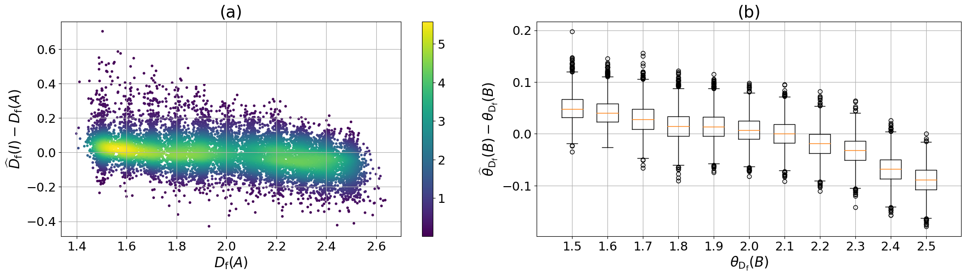
Figure 10: Estimation error of $\widehat{D}_{\mathrm{f}}$ (left) and $\widehat{\theta}_{\mathrm{D_{f}}}$ (right). In Subfigure (a) the quality of the prediction of the fractal dimension per aggregate is visualized, where the colors are computed by means of a Gaussian kernel density estimator. In Subfigure (b), the error regarding the prediction of the model parameter $\theta_{\mathrm{D_{f}}}$ is shown, where batches of size $\nu=12$ are used for the computation of $\widehat{\theta}_{\mathrm{D_{f}}}$.

3.2 Mixing ratio

To evaluate the accuracy of the estimator for the model parameter $\theta_{\mathrm{\uprho}}$, first, the image-wise straightforward case is considered, where the output $\mathrm{CNN_{reg}^{\rho}}(I)$ of the regression network is used as an estimator for the mixing ratio $\rho(A)$, without considering the classification network. As shown in Figure 11a, the output $\mathrm{CNN_{reg}^{\rho}}(I)$ of the regression network exhibits a relatively high bias for aggregates $A$ such that $\rho(A)\in[0,0.1]$ or $\rho(A)\in[0.9,1]$, with biases of about $0.04$ and $-0.1$, respectively.

To address this issue, in Section 2.3.3 a procedure which utilizes an additional classification network $\mathrm{CNN_{class}^{\rho}}$ is presented. In Figure 11b, the resulting image-wise error of $\widehat{\rho}$ using this procedure is shown. It is evident that the error of $\widehat{\rho}$ is significantly reduced for homogenous aggregates. More precisely, the bias of $\widehat{\rho}(I)$ for aggregates $A$ with $\rho(A)\in[0,0.1]$ or $\rho(A)\in[0.9,1]$ decreases to about 0.009 and 0.02, respectively. Incorporating the additional network, the MAE of the image-wise predicted mixing ratio $\widehat{\rho}(I)$ of an aggregate $A$ decreases from 0.059 to 0.053. Consequently, the MAE of the batch-wise prediction $\widehat{\theta}_{\mathrm{\uprho}}$ of $\theta_{\mathrm{\uprho}}$ improves significantly, reducing from $0.027$ to $0.017$.

Figure 11: Estimation error of $\widehat{\rho}$ (left, center) and $\widehat{\theta}_{\mathrm{\uprho}}$ (right). In Subfigure (a) the error of the unrounded output of the regression network is displayed per image. The black line, visualizing the mean error, is computed via a sliding window. The error for the output of the modified network is shown in Subfigure (b). In Subfigure (c) the error regarding the prediction of the model parameter $\theta_{\mathrm{\uprho}}$ is displayed, where the modified values of $\widehat{\rho}$ are used.

Note that the diagonally arranged points in Figure 11b are due to a small number of falsely classified heterogeneous aggregates, whereas the significantly thinned vertical lines are due to correctly classified homogeneous aggregates. The amounts of correctly and falsely classified aggregates are displayed in Table 4.

prediction \ true	homogenous	heterogeneous
homogenous	1 174	567
heterogeneous	67	12 082

Table 4: Confusion matrix of the homogeneous-heterogeneous classification task. About 95% of the aggregates are correctly classified.

3.3 Sizes of primary WO3 clusters and primary TiO2 clusters

Figure 12a shows the difference between the network output $\mathrm{CNN^{0}}(I(B))$ for the STEM images $I(B)=\{I_{i_{1}},\ldots,I_{i_{\nu}}\}$ corresponding to the aggregates $A_{i_{1}},\ldots,A_{i_{\nu}}$ in a batch $B$ (given in Eq. (15), i.e., prior to rounding of the output which would result in the estimator $\widehat{\theta}_{\mathrm{0}}$) and the preset value $\theta_{\mathrm{0}}(B)$ of the model parameter $\theta_{\mathrm{0}}$. Figure 12b shows the error distribution of $\widehat{\theta}_{\mathrm{0}}$ after rounding, where in about 48% of all cases the value of $\widehat{\theta}_{\mathrm{0}}$ coincides with $\theta_{\mathrm{0}}$. Additionally, in more than 92% of the cases, the error of $\widehat{\theta}_{\mathrm{0}}$ is less than or equal to 1. Although the largest mean absolute error occurs in the case of $\theta_{\mathrm{0}}=6$, the resulting inaccuracy corresponds to an average relative error of about $20\%$.

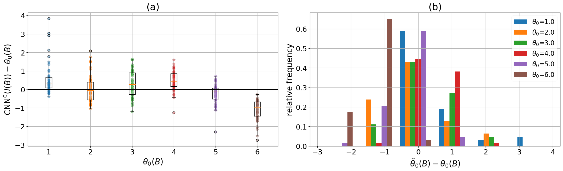
Figure 12: Estimation error of $\widehat{\theta}_{\mathrm{0}}$. In Subfigure (a), the differences between the network output $\mathrm{CNN^{0}}(I(B))$ and the preset values $\theta_{\mathrm{0}}(B)$ of the model parameter $\theta_{\mathrm{0}}$ are shown. The prediction error of $\widehat{\theta}_{\mathrm{0}}$ after applying the rounding operation is displayed in Subfigure (b).

The quality of the estimator $\widehat{\theta}_{\mathrm{1}}$ introduced in Section 2.3.5 is similar to that of $\widehat{\theta}_{\mathrm{0}}$, see Figure 13. After rounding the output of the network $\mathrm{CNN^{1}}$, 32% of the predictions coincided with the preset values of $\theta_{\mathrm{1}}$. In about 82% of the cases, an error less than or equal to 1 occurred. The mean absolute error for $\theta_{\mathrm{1}}=6$ is equal to $1.44$, where the resulting inaccuracy corresponds to an average relative error of about $24\%$.

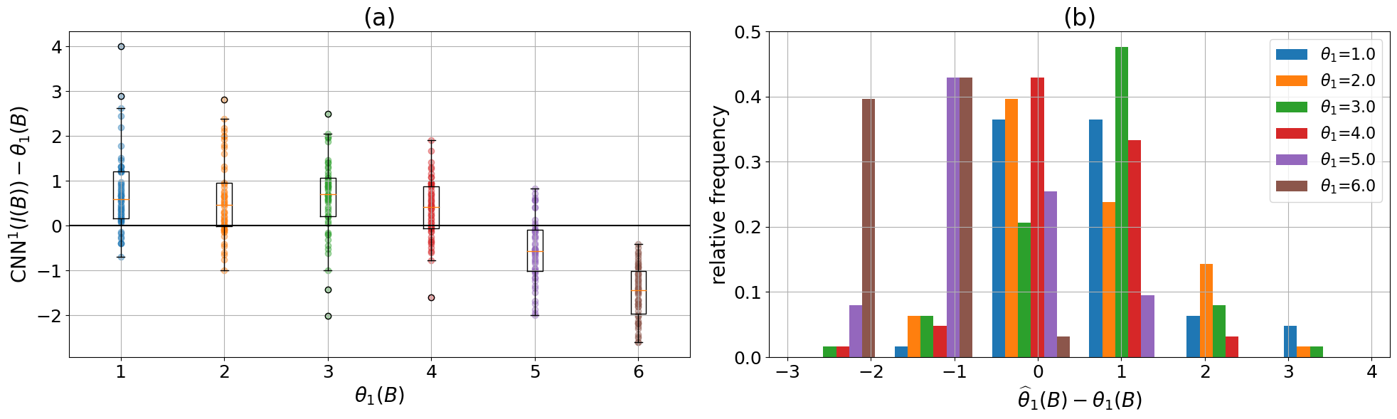
Figure 13: Estimation error of $\widehat{\theta}_{\mathrm{1}}$. In Subfigure (a), the differences between the network output $\mathrm{CNN^{1}}(I(B))$ and the preset values $\theta_{\mathrm{1}}(B)$ of the model parameter $\theta_{\mathrm{1}}$ are shown. The prediction error of $\widehat{\theta}_{\mathrm{1}}$ after applying the rounding operation is displayed in Subfigure (b).

3.4 Further structural descriptors of hetero-aggregates

Recall that the goal of the method presented in this paper is to generate realistic digital shadows of hetero-aggregates in 3D, solely from observations provided by 2D STEM images of the aggregates. For that purpose, the parameters ${\theta_{\mathrm{D_{f}}}},{\theta_{\mathrm{\uprho}}},{\theta_{\mathrm{0}}},{\theta_{\mathrm{1}}}$ of the stochastic 3D model introduced in Section 2.1.1 are predicted in order to specify the model configuration with which to generate digital shadows. However, so far, only the accuracy of the predictors ${\widehat{\theta}_{\mathrm{D_{f}}}},{\widehat{\theta}_{\mathrm{\uprho}}},{\widehat{\theta}_{\mathrm{0}}},{\widehat{\theta}_{\mathrm{1}}}$ for ${\theta_{\mathrm{D_{f}}}},{\theta_{\mathrm{\uprho}}},{\theta_{\mathrm{0}}},{\theta_{\mathrm{1}}}$ was evaluated, rather than investigating further structural descriptors of hetero-agggregates in order to evaluate the structural similarity between the resulting digital shadows and the original hetero-aggregates, i.e., the aggregates which were used for predicting the model parameters ${\theta_{\mathrm{D_{f}}}},{\theta_{\mathrm{\uprho}}},{\theta_{\mathrm{0}}},{\theta_{\mathrm{1}}}$. Moreover, many structural properties of the digital shadows are influenced by multiple model parameters, and thus, evaluating the quality of the four predictors ${\widehat{\theta}_{\mathrm{D_{f}}}},{\widehat{\theta}_{\mathrm{\uprho}}},{\widehat{\theta}_{\mathrm{0}}},{\widehat{\theta}_{\mathrm{1}}}$ separately is not sufficient. Therefore, three further structural descriptors, which characterize the 3D morphology of hetero-aggregates and have not yet been considered in this paper, are investigated in order to assess the similarity between original aggregates and corresponding digital shadows, see also Figure 1c-d.

3.4.1 Average cluster size and coordination numbers

The average cluster size $S_{\mathrm{\ce{TiO2}}}(A)$ of TiO2 particles of an aggregate $A=\{p_{i}=(x_{i},r_{i},l_{i}):x_{i}\in\mathbb{R}^{3},\leavevmode\nobreak\ r_{i}\in\mathbb{R}^{+},\leavevmode\nobreak\ l_{i}\in\{0,1\},\leavevmode\nobreak\ 1\leq i\leq N\}.$ describes the average cardinality of clusters of connected TiO2 particles in $A$. It is given by

$$S_{\mathrm{\ce{TiO2}}}(A)=\frac{1}{\#C_{\ce{TiO2}}(A)}\sum_{c\in C_{\ce{TiO2}}(A)}\#c,$$ (17)

where $C_{\ce{TiO2}}(A)$ denotes the set of all TiO2 clusters in $A$. While the value of $S_{\mathrm{\ce{TiO2}}}(A)$ is primarily influenced by the preset values of $\theta_{\mathrm{1}}$ and $\theta_{\mathrm{\uprho}}$, the value of $\theta_{\mathrm{0}}$ also has some (minor) influence on $S_{\mathrm{\ce{TiO2}}}(A)$ through its appearance in the definition of the Bernoulli-distributed labels $L_{k}$ of the stochastic 3D model, see Section 2.1.1.

Furthermore, the so-called average hetero-coordination number $Z_{\mathrm{hetero}}(A)$ of an aggregate $A$ is considered, which is given by

$$Z_{\mathrm{hetero}}(A) =\frac{1}{\text{\#$A$}}\sum_{p\in A}\#\{p^{\prime}\in A\colon p,p^{\prime}\text{ are in contact},l\not=l^{\prime}\}$$

$$=\frac{2\text{\#\{set of heterogeneous contacts in $A$\}}}{\text{\#$A$}}\,,$$ (18)

where #$A(=N)$ is the total number of particles in $A$. Thus, $Z_{\mathrm{hetero}}(A)$ is the average number of contacts of particles in $A$ with particles of the other material. Finally, the average coordination number $Z_{\mathrm{total}}(A)$, given by

$$Z_{\mathrm{total}}(A) =\frac{1}{\text{\#$A$}}\sum_{p\in A}\#\{p^{\prime}\in A\colon p,p^{\prime}\text{ are in contact}\}$$

$$=\frac{2\text{\#\{set of contacts in $A$\}}}{\text{\#$A$}}\,,$$ (19)

is considered, which is the average number of contacts of particles in $A$ to other particles, regardless of their material.

Since the number of contacts of a particle within an aggregate $A$ strongly depends on the shape of $A$, the model parameter $\theta_{\mathrm{D_{f}}}$ significantly influences the values of the descriptors $Z_{\mathrm{hetero}}(A)$ and $Z_{\mathrm{total}}(A)$. Further, $Z_{\mathrm{hetero}}(A)$ tends to increase with $\theta_{\mathrm{\uprho}}$ close to 0.5 and decreasing primary cluster sizes determined by $\theta_{\mathrm{0}}$ and $\theta_{\mathrm{1}}$.

3.4.2 Comparison of original hetero-aggregates and their digital shadows

To evaluate the quality of the predictor $\widehat{\theta}=(\widehat{\theta}_{\mathrm{D_{f}}},\widehat{\theta}_{\mathrm{\uprho}},\widehat{\theta}_{\mathrm{0}},\widehat{\theta}_{\mathrm{1}})$ in terms of the structural descriptors introduced in Section 3.4.1, 50 configurations of $\theta=(\theta_{\mathrm{D_{f}}},\theta_{\mathrm{\uprho}},\theta_{\mathrm{0}},\theta_{\mathrm{1}})$ were selected at random, out of the index set $E$ of evaluation data. For each of these numerical specifications of $\theta$, 800 new aggregates $A_{1},\ldots,A_{800}$ were drawn from the corresponding stochastic 3D model, and their structural descriptors $S_{\mathrm{\ce{TiO2}}}(A_{i}),Z_{\mathrm{hetero}}(A_{i})$ and $Z_{\mathrm{total}}(A_{i})$ for $i\in\{1,\ldots,800\}$ were computed. Furthermore, for each case, the (preset) ground-truth parameter vector $\theta$ has been estimated using the methods explained in Section 2.3. Then, for each of the 50 specifications of $\widehat{\theta}$, 800 additional aggregates $A_{1}^{\prime},\ldots,A_{800}^{\prime}$ and computed their structural descriptors $S_{\mathrm{\ce{TiO2}}}(A_{i}^{\prime}),Z_{\mathrm{hetero}}(A_{i}^{\prime})$ and $Z_{\mathrm{total}}(A_{i}^{\prime})$ for $i\in\{1,\ldots,800\}$ were generated. Figure 14 visualizes the distributions of these structural descriptors for four numerical specifications of $\theta$, where the aggregates $A_{1},\ldots,A_{800}$ and $A_{1}^{\prime},\ldots,A_{800}^{\prime}$ were generated using either the preset parameter vector $\theta$ (blue) or its prediction $\widehat{\theta}$ (orange), respectively.

Figure 14: Distribution of the structural descriptors $S_{\mathrm{\ce{TiO2}}}(A_{i})$ and $S_{\mathrm{\ce{TiO2}}}(A_{i}^{\prime})$ (left column), $Z_{\mathrm{hetero}}(A_{i})$ and $Z_{\mathrm{hetero}}(A_{i}^{\prime})$ (middle column), as well as $Z_{\mathrm{total}}(A_{i})$ and $Z_{\mathrm{total}}(A_{i}^{\prime})$ (right column) of the original aggregates $A_{i}$ (blue) and their digital shadows $A_{i}^{\prime}$ (orange), for four numerical specifications of $\theta$ and their predictions $\widehat{\theta}$. For computing the histograms, 20 equidistant bins have been employed which span the entire range of respective values on the $x$-axis.

Note that the gaps in the histograms of the average coordination numbers $Z_{\mathrm{total}}(A_{i})$ and $Z_{\mathrm{total}}(A_{i}^{\prime})$ (right column) are due to the limited size of the considered aggregates, see Section 2.1.2. More specifically, the average coordination numbers $Z_{\mathrm{total}}(A_{i})$ and $Z_{\mathrm{total}}(A_{i}^{\prime})$ given in Eq. (19), of aggregates $A_{i},A_{i}^{\prime}$ with sizes smaller than or equal to $80$, can only take values in the set

$$H=\{\frac{2q_{1}}{q_{2}}:q_{1},q_{2}\in\mathbb{N},q_{1}\leq q_{2}\leq 80\},$$ (20)

where $H\cap(1.975,2)=\emptyset$ because of the limited denominator $q_{2}$ on the right-hand side of Eq. (20).

Furthermore, note that the predictor $\widehat{\theta}$ for $\theta$ displayed in the top row of Figure 14 has a much smaller mean absolute error than the one displayed in the second row. Nevertheless, the latter (blue and orange) histograms show a higher agreement than those in the top row of Figure 14. Meaning that a high degree of similarity (in terms of MAE) of $\theta$ and $\widehat{\theta}$ does not necessarily imply a high degree of similarity of the resulting descriptor distributions.

We quantitatively analyzed this discrepancy between the distributions of the structural aggregate descriptors resulting from the preset configuration of model parameters and their prediction. For that purpose, the absolute difference of the means of these pairs of distributions were computed . For example, the mean values of $S_{\mathrm{\ce{TiO2}}}(A_{i})$ and $S_{\mathrm{\ce{TiO2}}}(A_{i}^{\prime})$ (vertical lines) in the top row of Figure 14 are equal to $5.38$ and $11.00$ for the preset parameter vector $\theta$ and its prediction $\widehat{\theta}$, respectively. This results in an absolute error of $5.62$. Over all 50 pairs of $\theta$ and $\widehat{\theta}$, a MAE error of $2.165$ is achieved, see also Table 5, where the MAEs for all three structural descriptors considered in this section are given as well as the corresponding coefficient of determination $R^{2}$ defined as

$$R^{2}(y,\widehat{y})=1-\frac{\mathrm{MSE}(y,\widehat{y})}{\mathrm{MSE}(y,\overline{y})}.$$

Here, the vectors $y=(y_{1},\ldots,y_{50}),\widehat{y}=(\widehat{y}_{1},\ldots,\widehat{y}_{50})\in\mathbb{R}^{50}$ consist of the mean values of the distributions of the given aggregate descriptor computed for the 50 preset specifications of $\theta$ and their predictions $\widehat{\theta}$. More precisely, for $j\in\{1,\ldots,50\}$, $y_{j}=\frac{1}{800}\sum_{i=1}^{800}\gamma(A_{ij})$ and $\widehat{y}_{j}=\frac{1}{800}\sum_{i=1}^{800}\gamma(A^{\prime}_{ij})$, where $\gamma$ stands for either $S_{\mathrm{\ce{TiO2}}},Z_{\mathrm{hetero}}$ or $Z_{\mathrm{total}}$, and $A_{ij},A^{\prime}_{ij}$ denote the $i$-th aggregate drawn from the $j$-th specification of $\theta$ and its prediction $\widehat{\theta}$, respectively. Furthermore, $\overline{y}=\frac{1}{50}\sum_{i=1}^{50}y_{i}$.

	$S_{\mathrm{\ce{TiO2}}}$	$Z_{\mathrm{hetero}}$	$Z_{\mathrm{total}}$
MAE	2.165	0.056	0.007
$R^{2}$	0.84	0.85	0.87

Table 5: Discrepancy between the mean values of the distributions of $S_{\mathrm{\ce{TiO2}}}$, $Z_{\mathrm{hetero}}$, and $Z_{\mathrm{total}}$, with respect to the mean absolute error MAE and the coefficient of determination $R^{2}$, computed for the 50 preset specifications of $\theta$ and their predictions $\widehat{\theta}$.

4 Discussion

The analysis of image data in order to determine the fractal dimension of finite aggregates has been a popular approach for some time. Two commonly used methods for this purpose are the box counting and sandbox methods, which are relatively simple image analysis tools [2]. These methods can provide meaningful structural information, but the quality of the results is highly dependent on the quality of the images. Specifically, high contrast and resolution are necessary to obtain clear STEM images from which accurate structural information can be extracted. However, in cases where a high fractal dimension is present, i.e., $D_{\mathrm{f}}(A)>2$, these classical methods have to be adopted to avoid problems with geometric opacity. There are attempts to solve this problem under certain conditions, see [26]. Although this difficulty can be observed in the slightly decreasing accuracy for values of $D_{\mathrm{f}}>2.2$, which has been obtained by the CNN-based approach proposed in the present paper, a satisfying accuracy was achieved even for high fractal dimensions, as shown in Figure 10a. Furthermore, the CNN approach works well independently of the aggregate size, see Figure 15a.

Probably the most comparable conventional method for determining the mixing ratio of an aggregate via its 2D STEM image, is based on determining the particle label of each pixel using a threshold value. More specifically, depending on the pixel intensity, the pixel is classified as TiO2, WO3 or background, and then, using the a priori known particle size distributions, a mixing ratio can be predicted. However, since the representation of thick TiO₂ particles or of many overlapping TiO₂ particles can have the same pixel intensity values as the representation of thin WO₃ particles, this threshold approach has a large source of errors [11]. The best appearing thresholds using a ”brute force” algorithm on a representative data were determined. This results in an MAE of 0.078 per aggregate when estimating the mixing ratio. Compared to the MAE of 0.053, see Section3.2, of the CNN approach described in the present paper, the error increases by 40% for the thresholding method described above. This is likely due to the increased values of pixel intensity which are caused by overlapping particles (see Figure 8), where these pixels with increased intensity values tend to be classified as WO3. Therefore, conventional threshold methods become increasingly inaccurate with an increasing number of overlapping particles, contrary to the behavior of the CNN approach proposed in the present paper, see Figure 15b.

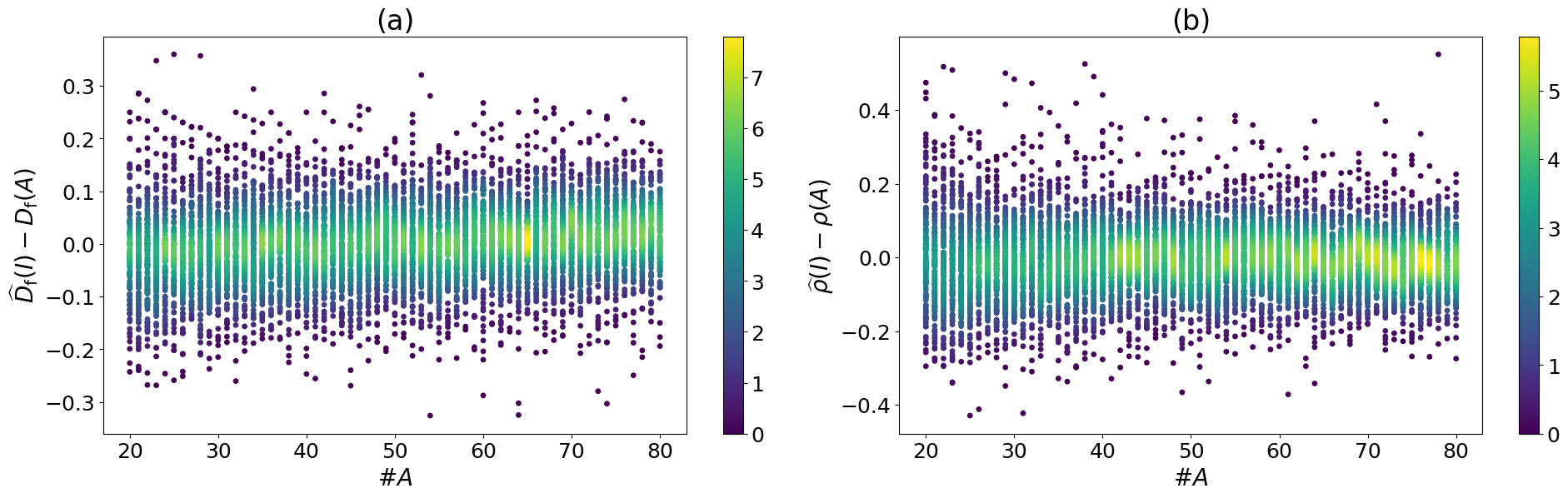
Figure 15: Prediction error for fractal dimension (left) and mixing ratio (right), depending on the number of particles per aggregate, for aggregates taken from the evaluation data given by the index set $E$. The color of dots is chosen according to a 1D Gaussian kernel density estimator along the $y$-axis.

Regarding the prediction of the remaining two model parameters $\theta_{\mathrm{0}}$ and $\theta_{\mathrm{1}}$, as far as we know, there is no comparable conventional method based on 2D image data. Such methods, if they do not consider depth information, would not be able to recognize if overlapping particles are touching or not, and thus, it is unlikely that they can accurately predict the values of $\theta_{\mathrm{0}}$ and $\theta_{\mathrm{1}}$.

Recall that the objective of the present paper is to generate digital shadows that are stochastically equivalent to the ground-truth aggregates used for model fitting. These digital shadows, which have known a 3D structure, can then be employed to predict the structural properties of the ground-truth aggregates at significantly reduced costs. Therefore, rather than just evaluating the accuracy of the predicted model parameters $\widehat{\theta}=(\widehat{\theta}_{\mathrm{D_{f}}},\widehat{\theta}_{\mathrm{\uprho}},\widehat{\theta}_{\mathrm{0}},\widehat{\theta}_{\mathrm{1}})$, the morphological similarities of the resulting digital shadows and their ground truth in terms of further structural descriptors, i.e., average clusters sizes and coordination numbers were also investigated. As already mentioned in Section 3.4.2, the MAE of $\widehat{\theta}$ is no appropriate tool to evaluate the similarity of digital shadows and their ground-truth aggregates. For instance, an extreme mixing ratio leads to a situation where the precision of either $\widehat{\theta}_{\mathrm{0}}$ or $\widehat{\theta}_{\mathrm{1}}$ has only a negligible impact on the structure of the resulting aggregates due to the corresponding material occurring very rarely. Moreover, the structural similarity of the resulting digital shadows is more strongly affected by small errors and rounding of $\mathrm{CNN^{0}}(I(B))$ and $\mathrm{CNN^{1}}(I(B))$ when the values of $\theta_{\mathrm{0}}$ and $\theta_{\mathrm{1}}$ are small, as opposed to when they are large. In particular, errors in the prediction of ground truths for small values of $\theta_{\mathrm{0}}$ and $\theta_{\mathrm{1}}$ result in higher relative errors. In such cases, large relative errors seem to have a greater impact on the structural discrepancies observed between aggregates generated for predicted and preset model parameters, see Figure 16. This effect can be further exacerbated by the application of subsequent rounding operations.

Figure 16: Distribution of the average heterogeneous coordination number $Z_{\mathrm{hetero}}(A)$ for three different values of $\theta_{\mathrm{0}}$. The dashed vertical lines show the mean value of $Z_{\mathrm{hetero}}(A)$ for each of the three specifications of $\theta_{\mathrm{0}}$, computed for a total of 2400 simulated aggregates $A$.

Although the predictor $\widehat{\theta}=(\widehat{\theta}_{\mathrm{D_{f}}},\widehat{\theta}_{\mathrm{\uprho}},\widehat{\theta}_{\mathrm{0}},\widehat{\theta}_{\mathrm{1}})$ proposed in this paper shows only minor discrepancies across all descriptors listed in Table 1, adapting the model and training process to address the issues mentioned above could enhance the similarity of digital shadows and original aggregates even further. For example, expanding the possible values of $\theta_{\mathrm{0}}$ and $\theta_{\mathrm{1}}$ to the interval $[1,6]$, rather than just considering the discrete set $\{1,2,\ldots,6\}$, would result in a diversity of aggregates, while also avoiding rounding errors that can arise in the prediction of $\theta_{\mathrm{0}}$ and $\theta_{\mathrm{1}}$. More specifically, this could be achieved by modifying the aggregation model $\Psi_{N^{\prime}}$ introduced in Eq. (7), such that the sizes of the primary clusters are randomly distributed, instead of choosing a constant cluster size. This would achieve a more detailed coverage of possible aggregate structures, especially for small values of $\theta_{\mathrm{0}}$ and $\theta_{\mathrm{1}}$. The training of CNNs could benefit from an adapted cost function that takes the values of other model parameters into account and assigns weights to errors based on the importance of the ground truth to be predicted.

5 Conclusion

A method has been developed in order to determine the parameters of a stochastic 3D model for synthetic TiO2-WO3 hetero-aggregates, based on their 2D STEM images. The method relies on convolutional neural networks that utilize distinct problem-specific architectures. If such an appropriately calibrated stochastic 3D model is available, the neural network approach bypasses the need for using traditional microstructure analysis and modeling techniques, which are expensive in time and costs, such as tomographic STEM imaging as well as complex image processing and segmentation. The networks were capable of predicting model parameters that describe fractal dimension, number-wise mixing ratio, and the sizes of primary clusters. The aggregates drawn from the stochastic 3D model with predicted model parameters exhibited almost the same coordination numbers and average cluster sizes as those generated by the model with the original (preset) parameters.

In the present paper, synthetic TiO2-WO3 hetero-aggregates are used as model system, because these two materials show a good material contrast in STEM images. However, only spherical particles were used for the generation of synthetic 3D aggregates. It would be interesting to investigate the effectiveness of the proposed method if particles for the hetero-aggregates are considered, which feature similar STEM intensities but differ significantly in their shape or size. Moreover, since experimentally measured aggregates feature more varied cluster sizes than synthetically generated ones, it can be presumed that a larger variability in cluster sizes would require more comprehensive data sets in order to make accurate predictions, but investigating this effect systematically is still important. Finally, in a forthcoming study, the presented method will be experimentally validated. More precisely, experimentally acquired 3D STEM image data of hetero-aggregates will be analyzed to investigate how well the stochastic 3D model proposed on the present paper can describe real aggregates.

6 Acknowledgements

This work was financially supported by the German Research Foundation (DFG) through the research grants RO 2057/17-1, MA 3333/25-1 and SCHM 997/42-1.

References

- [1] V. Baric, H. K. Grossmann, W. Koch, and L. Mädler. Quantitative characterization of mixing in multicomponent nanoparticle aggregates. Particle & Particle Systems Characterization, 35(10):1800177, 2018.
- [2] G. Bushell, Y. Yan, D. Woodfield, J. Raper, and R. Amal. On techniques for the measurement of the mass fractal dimension of aggregates. Advances in Colloid and Interface Science, 95(1):1–50, 2002.
- [3] J. Cai, N. Lu, and C. M. Sorensen. Analysis of fractal cluster morphology parameters: Structural coefficient and density autocorrelation function cutoff. Journal of Colloid and Interface Science, 171(2):470–473, 1995.
- [4] S. Chiu, D. Stoyan, W. Kendall, and J. Mecke. Stochastic Geometry and Its Applications. J. Wiley & Sons, 3rd edition, 2013.
- [5] R. Diehl, G. Brandt, and E. Salje. The crystal structure of triclinic WO3. Acta Crystallographica Section B, 34(4):1105–1111, 1978.
- [6] M. L. Eggersdorfer and S. E. Pratsinis. The structure of agglomerates consisting of polydisperse particles. Aerosol Science and Technology, 46(3):347–353, 2012.
- [7] M. L. Eggersdorfer and S. E. Pratsinis. Agglomerates and aggregates of nanoparticles made in the gas phase. Advanced Powder Technology, 25(1):71–90, 2014.
- [8] A. Filippov, M. Zurita, and D. Rosner. Fractal-like aggregates: Relation between morphology and physical properties. Journal of Colloid and Interface Science, 229(1):261–273, 2000.
- [9] S. R. Forrest and T. A. Witten. Long-range correlations in smoke-particle aggregates. Journal of Physics A: Mathematical and General, 12(5):L109, 1979.
- [10] M. Frei and F. E. Kruis. Image-based size analysis of agglomerated and partially sintered particles via convolutional neural networks. Powder Technology, 360:324–336, 2020.
- [11] B. Gerken, C. Mahr, J. Stahl, T. Grieb, M. Schowalter, F. F. Krause, T. Mehrtens, L. Mädler, and A. Rosenauer. Material discrimination in nanoparticle hetero-aggregates by analysis of scanning transmission electron microscopy images. Particle & Particle Systems Characterization, 40(9):2300048, 2023.
- [12] P. Gilbert. Iterative methods for the three-dimensional reconstruction of an object from projections. Journal of Theoretical Biology, 36(1):105 – 117, 1972.
- [13] I. Goodfellow, Y. Bengio, and A. Courville. Deep Learning. MIT Press, 2016.
- [14] M. Horn and C. P. Schwerdtfeger. Refinement of the structure of anatase at several temperatures. Zeitschrift für Kristallographie, 136(3-4):273–281, 1972.
- [15] S. Ioffe and C. Szegedy. Batch normalization: Accelerating deep network training by reducing internal covariate shift. In International conference on machine learning, pages 448–456. pmlr, 2015.
- [16] G. James, D. Witten, T. Hastie, and R. Tibshirani. An Introduction to Statistical Learning. Springer, 2nd edition, 2021.
- [17] L. Jones and P. D. Nellist. Identifying and correcting scan noise and drift in the scanning transmission electron microscope. Microscopy and Microanalysis, 19(4):1050–1060, 05 2013.
- [18] Jullien, R., Kolb, M., and Botet, R. Aggregation by kinetic clustering of clusters in dimensions d 2. Journal de Physique Lettres, 45(5):211–216, 1984.
- [19] S. Kench and S. J. Cooper. Generating three-dimensional structures from a two-dimensional slice with generative adversarial network-based dimensionality expansion. Nature Machine Intelligence, 3(4):299–305, 2021.
- [20] D. Kingma and J. Ba. Adam: A method for stochastic optimization. In Y. Bengio and Y. Le Cun, editors, Proceedings of the 3rd International Conference on Learning Representations, 2015.
- [21] E. J. Kirkland. Advanced Computing in Electron Microscopy. Springer, 1998.
- [22] T. Kirstein, L. Petrich, R. R. P. Purushottam Raj Purohit, J.-S. Micha, and V. Schmidt. CNN-based laue spot morphology predictor for reliable crystallographic descriptor estimation. Materials, 16:3397, 2023.
- [23] F. F. Krause, M. Schowalter, T. Grieb, K. Müller-Caspary, T. Mehrtens, and A. Rosenauer. Effects of instrument imperfections on quantitative scanning transmission electron microscopy. Ultramicroscopy, 161:146–160, 2016.
- [24] B. O. Loopstra and H. M. Rietveld. Further refinement of the structure of WO3. Acta Crystallographica Section B, 25(7):1420–1421, 1969.
- [25] J. Low, J. Yu, M. Jaroniec, S. Wageh, and A. A. Al-Ghamdi. Heterojunction photocatalysts. Advanced Materials, 29(20):1601694, 2017.
- [26] F. Maggi and J. C. Winterwerp. Method for computing the three-dimensional capacity dimension from two-dimensional projections of fractal aggregates. Physical Review E, 69:011405, 2004.
- [27] P. Meakin. Formation of fractal clusters and networks by irreversible diffusion-limited aggregation. Physical Review Letters, 51:1119–1122, 1983.
- [28] P. Midgley and M. Weyland. 3D electron microscopy in the physical sciences: the development of Z-contrast and EFTEM tomography. Ultramicroscopy, 96(3):413 – 431, 2003.
- [29] R. Mohammed, J. Rawashdeh, and M. Abdullah. Machine learning with oversampling and undersampling techniques: Overview study and experimental results. In 11th International Conference on Information and Communication Systems (ICICS), pages 243–248, 2020.
- [30] M. Neumann, J. Staněk, O. M. Pecho, L. Holzer, V. Beneš, and V. Schmidt. Stochastic 3D modeling of complex three-phase microstructures in sofc-electrodes with completely connected phases. Computational Materials Science, 118:353–364, 2016.
- [31] M. Neumann, S. E. Wetterauer, M. Osenberg, A. Hilger, P. Gräfensteiner, A. Wagner, N. Bohn, J. R. Binder, I. Manke, T. Carraro, and V. Schmidt. A data-driven modeling approach to quantify morphology effects on transport properties in nanostructured NMC particles. International Journal of Solids and Structures, 280:112394, 2023.
- [32] K. K. Pal and K. S. Sudeep. Preprocessing for image classification by convolutional neural networks. In 2016 IEEE International Conference on Recent Trends in Electronics, Information & Communication Technology (RTEICT), pages 1778–1781, 2016.
- [33] J. A. Pinedo-Escobar, J. Fan, E. Moctezuma, C. Gomez-Solís, C. J. Carrillo Martinez, and E. Gracia-Espino. Nanoparticulate double-heterojunction photocatalysts comprising TiO2(Anatase)/WO3/TiO2(Rutile) with enhanced photocatalytic activity toward the degradation of methyl orange under near-ultraviolet and visible light. ACS Omega, 6(18):11840–11848, 2021.
- [34] B. Prifling, M. Neumann, D. Hlushkou, C. Kübel, U. Tallarek, and V. Schmidt. Generating digital twins of mesoporous silica by graph-based stochastic microstructure modeling. Computational Materials Science, 187:109934, 2021.
- [35] A. Rosenauer and M. Schowalter. STEMSIM - a new software tool for simulation of STEM HAADF Z-contrast imaging. In A. Cullis and P. Midgley, editors, Microscopy of Semiconducting Materials 2007, volume 120 of Springer Proceedings in Physics, pages 170–172. Springer, 2008.
- [36] C. F. G. D. Santos and J. P. Papa. Avoiding overfitting: A survey on regularization methods for convolutional neural networks. ACM Computing Surveys, 54:213, 2022.
- [37] P. Simard, D. Steinkraus, and J. Platt. Best practices for convolutional neural networks applied to visual document analysis. In Seventh International Conference on Document Analysis and Recognition, pages 958–963, 2003.
- [38] K. Sugiyama and Y. Takéuchi. The crystal structure of rutile as a function of temperature up to 1600∘C. Zeitschrift für Kristallographie - Crystalline Materials, 194(1-4):305–314, 1991.
- [39] T. Szandała. Review and comparison of commonly used activation functions for deep neural networks. arXiv preprint arXiv:2010.09458, 2020.
- [40] Y. Tae Kwon, K. Yong Song, W. In Lee, G. Jin Choi, and Y. Rag Do. Photocatalytic behavior of WO3-loaded TiO2 in an oxidation reaction. Journal of Catalysis, 191(1):192–199, 2000.
- [41] D. Van Dyck. Is the frozen phonon model adequate to describe inelastic phonon scattering? Ultramicroscopy, 109(6):677 – 682, 2009.
- [42] M. Weber, A. Grießer, E. Glatt, A. Wiegmann, and V. Schmidt. Modeling curved fibers by fitting R-vine copulas to their frenet representations. Microscopy and Microanalysis, 29(1):155–165, 2023.
- [43] X. Yan, X. Zong, G. Q. M. Lu, and L. Wang. Ordered mesoporous tungsten oxide and titanium oxide composites and their photocatalytic degradation behavior. Progress in Natural Science: Materials International, 22(6):654–660, 2012.