Practical trainable temporal post-processor for multi-state quantum measurement

Abstract

We develop and demonstrate a trainable temporal post-processor (TPP) harnessing a simple but versatile machine learning algorithm to provide optimal processing of quantum measurement data subject to arbitrary noise processes, for the readout of an arbitrary number of quantum states. We demonstrate the TPP on the essential task of qubit state readout, which has historically relied on temporal processing via matched filters in spite of their applicability only for specific noise conditions. Our results show that the TPP can reliably outperform standard filtering approaches under complex readout conditions, such as high power readout. Using simulations of quantum measurement noise sources, we show that this advantage relies on the TPP’s ability to learn optimal linear filters that account for general quantum noise correlations in data, such as those due to quantum jumps, or correlated noise added by a phase-preserving quantum amplifier. Furthermore, for signals subject to Gaussian white noise processes, the TPP provides a linearly-scaling semi-analytic generalization of matched filtering to an arbitrary number of states. The TPP can be efficiently, autonomously, and reliably trained on measurement data, and requires only linear operations, making it ideal for FPGA implementations in cQED for real-time processing of measurement data from general quantum systems.

I Introduction

High fidelity quantum measurement is essential for any quantum information processing scheme, from quantum computation to quantum machine learning. However, while measurement optimization has focused on quantum hardware advancements [1, 2, 3], several modern experiments operate in regimes where optimal hardware conditions are difficult to sustain, or - for machine learning with general quantum systems [4, 5, 6, 7, 8] - may not always be known. For example, in the push towards higher qubit readout fidelities with complex multi-qubit processors in circuit QED (cQED), optimization of individual readout resonators becomes increasingly difficult. More importantly, finite qubit coherence means that simply extending the measurement duration is not a viable option to enhance fidelity: faster and hence higher power measurements are needed. However, these readout powers are associated with enhanced qubit transitions, leading to the $T_{1}$ versus $\bar{n}$ problem [9, 10, 11, 12, 13, 14] and excitation to higher states [15, 14] outside the computational subspace. Machine learning with quantum devices operating in unconventional regimes allows for an even broader range of complex dynamics. Quantum measurement data obtained under these conditions cannot be expected to be optimally analyzed using schemes built for more standard readout paradigms [16]. Therefore, a practical approach to extract the maximum information possible from such data is timely.

In this paper, we demonstrate a machine learning scheme to optimally process quantum measurement data for completely general quantum state classification tasks. For the most common such task of qubit state readout, standard post-processing of measurement records has remained relatively unchanged (with some exceptions [17, 18]): data is filtered using a “matched filter” (MF) constructed from the mean of measurement records for two states to be distinguished (for example, states $\ket{e}$ or $\ket{g}$ of a qubit). Crucially, the MF thus defined applies only to binary classification, and much more restrictively is optimal only if readout is subject to Gaussian white (i.e. uncorrelated) noise process [19]. In many cases, an even simpler (and less optimal) boxcar filter is employed, due to the ease of its construction. Our approach harnesses machine learning to provide a model-free trainable temporal post-processor (TPP) of quantum measurement data in general noise conditions, and for an arbitrary number of states of a generic measured quantum system ( for source code). We test our approach by applying it to the experimental readout of distinct qubits across a range of measurement powers. Our results show that the TPP reliably outperforms the standard MF under complex readout conditions at high powers, providing in certain cases a reduction in errors by a factor of several. Furthermore, the TPP achieves this improvement while requiring only linear weights applied to quantum measurement data (see Fig. 1): this makes it compatible with FPGA implementations for real-time hardware processing, and exacts a lower training cost than neural network-based machine learning schemes [21, 22].

Machine learning has already been established as a powerful approach to classical temporal data processing, providing state-of-the-art fidelity in tasks such as time series prediction [23], and chaotic systems’ forecasting [24, 25, 26] and control [27]. Adapting this approach to quantum state classification as we do here requires its application to time-evolving quantum signals. Signals extracted from the readout of quantum systems are often dominated by noise, making their processing distinct from that required of typical data from classical systems. More importantly, the noise in such signals can arise from truly quantum-mechanical sources, such as stochastic transitions between states of a multi-level atom (quantum ‘jumps’), or vacuum fluctuations in quantum modes. A key finding of our work is that the TPP is able to learn from precisely these quantum noise correlations in data extracted from quantum systems to improve classification fidelity. To uncover this essential principle of TPP learning, we first develop an interpretation of the TPP as the application of optimal filters to quantum measurement data. This provides a framework to quantify and visualize what is ‘learnt’ by the TPP from a given dataset. Secondly, TPP learning is tested on simulated quantum measurement datasets using stochastic master equations, where quantum noise sources and hence their correlation signatures in measured data can be precisely controlled.

Using simulated datasets where all noise sources contribute additive Gaussian white noise - a reasonable assumption for measurement chains under ideal conditions - we show that the TPP provides filters that reduce exactly to the matched filter for binary classification. More importantly, as the TPP is valid for the classification of any number of states, it provides the generalization of matched filters for arbitrary state classification. We then provide a systematic analysis of TPP applied to quantum measurement with more complex quantum noise sources, such as quantum amplifiers adding correlated quantum noise, or noise due to state transitions. In such scenarios, the TPP filters can deviate substantially from filters learned under the white noise assumption. Crucially, these noise-adapted TPP filters outperform generalized matched filters. By learning from quantum noise correlations, the TPP therefore utilizes a characteristic of quantum measurement data inaccessible to post-processing schemes relying on noise-agnostic matched filtering methods.

The established learning principles provide a structure to the general applicability of the TPP, which we believe enhances its practical utility. First, the exact mapping to matched filters under appropriate noise conditions places the TPP on firm footing, guaranteed to perform at least as well as these baseline methods. Secondly, and much more importantly, the TPP’s ability to learn from noise (crucially, quantum noise) renders it able to then beat the MF when noise conditions change. This theoretical adaptability becomes practical due to the TPP’s straightforward training procedure, which is also ideal for autonomous repeated calibrations, necessary on even industrial-grade quantum processors [28, 29, 30]. Ultimately, the trainable TPP could provide an ideal component to optimally process quantum measurement data from general quantum devices used for machine learning, which could exhibit exotic quantum noise characteristics.

The rest of this paper is organized as follows. In Sec. II we introduce the quantum measurement task we use as an example to demonstrate the TPP: dispersive qubit readout in the cQED architecture. In Sec. III we then introduce our temporal post-processing framework to multi-state classification: a model-free supervised machine learning approach that can be applied to the classification of arbitrary time series. Importantly, we draw connections between the TPP approach and standard filtering-based approaches to qubit state measurement. In Sec. IV, we apply the developed TPP framework to experimental data for qubit readout, showing that it can outperform standard matched-filtering at strong measurement powers relevant for high-fidelity readout. Sec. V delves into the aspects that enable the TPP to learn filters that can be more effective than standard matched filters using controlled simulations. We conclude with a discussion on the general applicability of TPP for quantum state classification and temporal processing of quantum measurement data.

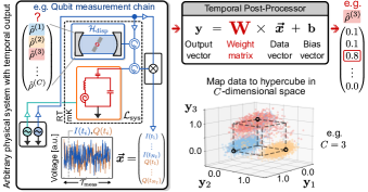
Figure 1: Temporal post-processor (TPP) for multi-state classification using quantum measurement data, demonstrated for dispersive qubit readout in cQED. The objective is to process temporal data corresponding to an unknown state (indexed $\sigma$) of an arbitrary physical system - here the state of a qubit in a quantum measurement chain - to estimate the true label $\sigma$ with maximum accuracy. The TPP approach uses a set of weights $\mathbf{W}$ and biases $\mathbf{b}$ to map the vector $\bm{\vec{x}}$ of measured data, comprising an instance of $N_{\rm O}$ observables each a time series of length $N_{\rm T}$, to the corners of a hypercube in $C$-dimensional space. Optimal values of $\mathbf{W}$ and $\mathbf{b}$ are learned by training to realize this mapping with minimal error, in a least-squares sense. Scatter plots shown in $C=3$ dimensional space are data from real qubit $p\in\{e,g,f\}$ readout after the TPP.

II Standard post-processing for dispersive qubit readout

II.1 Quantum measurement chain for dispersive qubit readout

The standard quantum measurement chain for heterodyne readout in cQED is depicted schematically in Fig. 1, and can be modeled via the stochastic master equation (SME):

$$d\hat{\rho}_{c}=\mathcal{L}_{\rm sys}\hat{\rho}_{c}\leavevmode\nobreak\ dt+\mathcal{L}_{\rm envt}\hat{\rho}_{c}\leavevmode\nobreak\ dt+\mathcal{L}_{\rm meas}[dW]\hat{\rho}_{c}.$$ (1)

Here the Liouvillian superoperator $\mathcal{L}_{\rm sys}$ defines the quantum system whose states are to be read out. We emphasize that the TPP approach enables classification for completely general $\mathcal{L}_{\rm sys}$. For relevance to cQED applications, in this paper we choose to focus on dispersive qubit readout, where the system comprises a multi-level artificial atom (here, a transmon) dispersively coupled to a readout cavity that is driven using a coherent tone at frequency $\omega_{d}$. Then, $\mathcal{L}_{\rm sys}\hat{\rho}=-i[\hat{\mathcal{H}}_{\rm disp},\hat{\rho}]$, where the dispersive Hamiltonian $\hat{\mathcal{H}}_{\rm disp}$ for a multi-level transmon takes the form (for cavity operators in the interaction frame with respect to $\omega_{d}$ and setting $\hbar=1$)

$$\hat{\mathcal{H}}_{\rm disp}\simeq\sum_{p}\omega_{p}|p\rangle\!\langle p|-\Delta_{da}\hat{a}^{\dagger}\hat{a}+\sum_{p}\chi_{p}\hat{a}^{\dagger}\hat{a}|p\rangle\!\langle p|.$$ (2)

Here $\Delta_{da}=\omega_{d}-\omega_{a}$ is the detuning between the cavity and the readout tone at frequency $\omega_{d}$, while $\chi_{p}$ is the dispersive shift per photon when the artificial atom is in state $\ket{p}$ [31, 32]. The general Liouvillian $\mathcal{L}_{\rm envt}$ is then used to describe all losses through channels that are not directly monitored, such as transmon transitions.

The final superoperator $\mathcal{L}_{\rm meas}$ defines measurement chain components that are actively monitored to read out the state of the quantum system of interest. Here, we consider continuous heterodyne monitoring of a single quantum mode of the measurement chain, generally labelled $\hat{d}$. In the simplest case, $\mathcal{L}_{\rm meas}$ defines readout of the cavity itself (then, $\hat{d}\to\hat{a}$); however, it can also describe the dynamics (coherent or otherwise) of any other monitored quantum devices in the measurement chain. The most pertinent example is readout of the signal mode of an (ideally linear) quantum-limited amplifier that follows the dispersive qubit-cavity system via an intermediate circulator, as shown schematically in Fig. 1. Most generally, $\mathcal{L}_{\rm meas}$ can describe the monitoring of several modes of a general quantum nonlinear processor that is embedded in the measurement chain [5]. Crucially, $\mathcal{L}_{\rm meas}$ must include a stochastic component (indicated by the Wiener increment $dW$), describing measurement-conditioned dynamics of the dispersive qubit-cavity system under such continuous monitoring (see Appendix B).

For a qubit in the (a priori unknown) initial state $\ket{\sigma}$ before measurement, continuous monitoring of the measurement chain then yields a single ‘shot’ of heterodyne records $\{I^{(\sigma)}(t),Q^{(\sigma)}(t)\}$ contingent on this state $\sigma$. The complexity of this readout task can be appreciated given the form of raw heterodyne records even under a simplified theoretical model:

$$I^{(\sigma)}(t_{i}) =\sqrt{\kappa}\langle\hat{X}^{(\sigma)}(t_{i})\rangle_{c}+\xi_{I}(t_{i})+\xi_{I}^{\rm cl}(t_{i}),$$ (3a)

$$Q^{(\sigma)}(t_{i}) =\sqrt{\kappa}\langle\hat{P}^{(\sigma)}(t_{i})\rangle_{c}+\xi_{Q}(t_{i})+\xi_{Q}^{\rm cl}(t_{i}).$$ (3b)

We consider discretized temporal indices $t_{i}$, for $i\in[N_{\rm T}]$ and $N_{\rm T}=\mathcal{T}_{\rm meas}/\Delta t$, where $\mathcal{T}_{\rm meas}$ is the total measurement time and $\Delta t$ is the sampling time set by the digitizer. Heterodyne measurement probes the canonical quadratures $\hat{X}=\frac{1}{\sqrt{2}}(\hat{d}+\hat{d}^{\dagger})$, $\hat{P}=\frac{-i}{\sqrt{2}}(\hat{d}-\hat{d}^{\dagger})$ of the mode $\hat{d}$ being monitored. More precisely, $\langle\hat{X}^{(\sigma)}(t_{i})\rangle_{c},\langle\hat{P}^{(\sigma)}(t_{i})\rangle_{c}$ describe individual quantum trajectories of measured quadratures, conditioned on measurement records via a dependence on the heterodyne measurement noise $\xi_{I/Q}(t_{i})$ through $\mathcal{L}_{\rm meas}$. The heterodyne measurement noise itself is modelled as zero-mean Gaussian white noise,

$$\mathbb{E}[\xi_{I,Q}(t_{i})]=0,\leavevmode\nobreak\ \leavevmode\nobreak\ \mathbb{E}[\xi_{I,Q}(t_{i})\xi_{I,Q}(t_{j})]=\frac{1}{\Delta t}\delta_{ij}\delta_{I,Q}$$ (4)

where $\mathbb{E}[\cdot]$ describes ensemble averages over distinct noise realizations (obtained for distinct measurements). In contrast, the quantum trajectories contain the quantum noise contributions to the measurement records, in addition to state information: these include amplified quantum fluctuations when measuring the output field from a quantum amplifier, or the influence of quantum jumps in the measured cavity field due to transitions of the dispersively coupled qubit.

Finally, $\xi_{I/Q}^{\rm cl}(t_{i})$ describe classical noise contributions to measurement records, for example noise added by classical HEMT amplifiers. While the statistics of this noise may take different forms, they are formally distinct from heterodyne measurement noise as they are not associated with a stochastic measurement superoperator in Eq. (1).

The objective of the readout task is then to use this noisy temporal measurement data to obtain an estimated class label $\sigma^{\rm est}$ that is ideally equal to the true class label $\sigma$. Furthermore, we require single-shot readout [33], where the estimation must be performed using only a single measurement shot: such rapid readout is essential for quantum feedback and control applications [34, 35, 36].

II.2 Binary qubit state measurement and matched filters

The standard classification paradigm in cQED to obtain $\sigma^{\rm est}$ from raw heterodyne records would formally be described as a filtered Gaussian discriminant analysis (FGDA) in contemporary learning theory. This comprises two stages: (i) temporal filtering of each measured quadrature, and (ii) assigning a class label to filtered quadratures that maximises the likelihood of their observation amongst all $C$ classes as determined by a Gaussian probability density function. Formally, this procedure can be written as:

$$\sigma^{\rm est}={\rm G}\!\left[\sum_{i}\begin{pmatrix}h_{I}(t_{i})I^{(\sigma)}(t_{i})\\ h_{Q}(t_{i})Q^{(\sigma)}(t_{i})\end{pmatrix}\right]={\rm G}\!\left[\begin{pmatrix}\vec{h}_{I}^{T}\vec{I}^{(\sigma)}\!\\ \vec{h}_{Q}^{T}\vec{Q}^{(\sigma)}\!\end{pmatrix}\right]$$ (5)

where in the second expression we have introduced vectorized notation in the space of measurement records, so that $\vec{I}_{i}=I(t_{i})$, enabling the filtering step to be written as an inner product. The function ${\rm G}\!\left[\cdot\right]$ then assigns class labels according to the aforementioned Gaussian discriminator.

A fact seldom mentioned explicitly is that both the temporal filters and the Gaussian discriminator must be constructed using a calibration dataset: a set of $N_{\rm train}$ heterodyne records obtained when the initial qubit states are known under controlled initialization protocols. For example, for the most commonly considered case of binary qubit state classification to distinguish states $\ket{e}$ and $\ket{g}$, and under the assumption that the noise in heterodyne records is additive Gaussian white noise, an optimal filter is known: the matched filter [37, 19, 38]. The empirical matched filter is constructed from the calibration dataset, where $(n)$ indexes distinct records, via

$$\vec{h}_{I}=\frac{1}{N_{\rm train}}\sum_{n=1}^{N_{\rm train}}\left(\vec{I}_{(n)}^{(e)}-\vec{I}_{(n)}^{(g)}\right)$$ (6)

with $\vec{h}_{Q}$ defined analogously with $I\to Q$. The function ${\rm G}\!\left[\cdot\right]$ requires fitting Gaussian profiles to measured probability distributions of known classes, and hence uses means and variances estimated from calibration data.

While a Gaussian discriminant analysis can be applied to classification of an arbitrary number of states $C$ and beyond white noise constraints, the choice of an optimal temporal filter in these more general situations is not straightforward [39]. Due to their ease of construction, often a matched filter akin to Eq. (6), or an even more rudimentary boxcar filter (a uniform filter that is nonzero only when the measurement signal is on) are deployed, regardless of the complexity of the noise conditions (for example, when qubit decay is significant and more optimal filters can be found [19]). We will show how the TPP approach provides a natural generalization of matched filtering to multi-state classification, and furnishes a trainable classifier that can generalize to more complex noise environments.

III Trainable temporal post-processor for multi-state classification

Machine learning using only linear trainable weights has shown remarkable success in time-dependent supervised machine learning tasks [21]. In such cases, the objective is to map a time series faithfully to a dynamically-evolving target function via the application of an efficiently trainable linear transformation [22]. Here, we adapt this framework to processing of temporal measurement data from a quantum system and with a time-independent target, as is relevant for initial state classification [19].

To overview its key features we first introduce the mathematical framework underpinning the TPP, which is defined as follows. We consider $N_{\rm O}$ continuously measured observables, each measurement yielding a time series of length $N_{\rm T}$. All measured data corresponding to an unknown state with index $\sigma$ can be compiled into the vector $\bm{\vec{x}}^{(\sigma)}$ which thus exists in the space $\bm{\vec{x}}^{(\sigma)}\in\mathbb{R}^{N_{\rm O}\cdot N_{\rm T}}$. As an example, in the case of heterodyne measurement, $N_{\rm O}=2$ and $\bm{\vec{x}}^{(\sigma)}=\begin{pmatrix}\vec{I}^{(\sigma)}\\ \vec{Q}^{(\sigma)}\end{pmatrix}$ (see Fig. 1).

Formally, operation of the TPP is then described as an input-output transformation, mapping a vector $\bm{\vec{x}}^{(\sigma)}$ from the space of measured data, $\mathbb{R}^{N_{\rm O}\cdot N_{\rm T}}$, to a vector $\mathbf{y}\in\mathbb{R}^{C}$ in the space of class labels; the scalar predicted class label $\sigma^{\rm est}$ is given by an operation ${\rm F}\!\left[\cdot\right]$ on this vector $\mathbf{y}$, so that the complete transformation is:

$$\sigma^{\rm est}={\rm F}\!\left[\mathbf{y}\right]={\rm F}\!\left[\mathbf{W}\bm{\vec{x}}^{(\sigma)}+\mathbf{b}\right]$$ (7)

The function ${\rm F}\!\left[\cdot\right]$ is often taken to be the ${\rm argmax}\{\cdot\}$ function that extracts the position of the largest element in $\mathbf{y}$. However, it can also be a suitably-trained Gaussian discriminator ${\rm G}\!\left[\cdot\right]$ as in Eq. (5). The dimensions of the various components making up the TPP framework are summarized in Table 1.

Table 1: Summary of components of the TPP learning framework and their dimensions.

Component and dimensions
TPP output	$\mathbf{y}$	$\mathbb{R}^{C}$
Weights	$\mathbf{W}$	$\mathbb{R}^{C\times(N_{\rm O}\cdot N_{\rm T})}$
Data	$\bm{\vec{x}}$	$\mathbb{R}^{N_{\rm O}\cdot N_{\rm T}}$
Bias	$\mathbf{b}$	$\mathbb{R}^{C}$
Data means, state $p$	$\bm{\vec{s}}^{(p)}$	$\mathbb{R}^{N_{\rm O}\cdot N_{\rm T}}$
Noise process, state $p$	$\bm{\vec{\zeta}}^{(p)}$	$\mathbb{R}^{N_{\rm O}\cdot N_{\rm T}}$
“Gram” matrix	$\mathbf{G}$	$\mathbb{R}^{(N_{\rm O}\cdot N_{\rm T})\times(N_{\rm O}\cdot N_{\rm T})}$
Correlation matrix	$\mathbf{V}$	$\mathbb{R}^{(N_{\rm O}\cdot N_{\rm T})\times(N_{\rm O}\cdot N_{\rm T})}$

We note that at first sight Eq. (7), which defines the TPP scheme for classification, appears to be analogous to Eq. (5) in the FGDA scheme. There are, in fact, close connections between the two, as we will expand upon shortly. However, the TPP framework is also markedly different, in what can broadly be categorized as two aspects.

First, the defining feature of any machine learning approach: the ability (and requirement) to learn from data. $\mathbf{W}\in\mathbb{R}^{C\times N_{\rm O}\cdot N_{\rm T}}$ is a trainable matrix of weights and $\mathbf{b}\in\mathbb{R}^{C}$ is a vector of trainable biases, both learned from data $\bm{\vec{x}}^{(p)}$ with known labels $p$ ($C$ in total) in a supervised learning framework. More precisely, the target $\mathbf{y}\in\mathbb{R}^{C}$ for any instance of $\bm{\vec{x}}^{(p)}$ is taken to be a vector with only one nonzero element - a single $1$ at index $p$, defining a corner of a $C$-dimensional hypercube (referred to as one-hot encoding, see Fig. 1). Then, the optimal $\mathbf{W}^{\rm opt},\mathbf{b}^{\rm opt}$ minimize a least-squares cost function to achieve this target with minimal error:

$$\{\mathbf{W}^{\rm opt},\mathbf{b}^{\rm opt}\}=\underset{\mathbf{W},\mathbf{b}}{\rm argmin}||\mathbf{Y}-\left(\mathbf{W}\mathbf{X}+\mathbf{b}\right)||^{2}$$ (8)

Here $\mathbf{X}$ is the matrix containing the complete training dataset, comprising $N_{\rm train}$ instances of $\bm{\vec{x}}^{(p)}$ for each class $p$, while $\mathbf{Y}$ is the corresponding set of targets (see Appendix C for full training details). The FGDA scheme using matched filters is in principle tailored to situations where useful signal in data is obscured only by additive Gaussian white noise, although it is applied much more broadly in practice. The TPP places no such restrictions on the training data a priori, and can therefore generalize to more nontrivial noise conditions, as we will show. Furthermore, a distinguishing feature of the TPP framework amongst other ML paradigms is that its optimization is convex and hence guaranteed to converge.

The second defining feature is the scope of applicability of the TPP framework. It natively generalizes to the classification of an arbitrary number of states $C$. Furthermore, no restriction is placed on the type of data that constitutes the vector $\bm{\vec{x}}$. In particular, no underlying physical model of the system generating the measurement data is a priori required: any relevant information must be learned by the TPP from data during the training phase. This also implies that the results in this paper apply to the classification of time series that have nothing to do with qubit state measurement. Its generality and ease of training enable the TPP to serve as a versatile trainable classifier, suited to a variety of classification tasks.

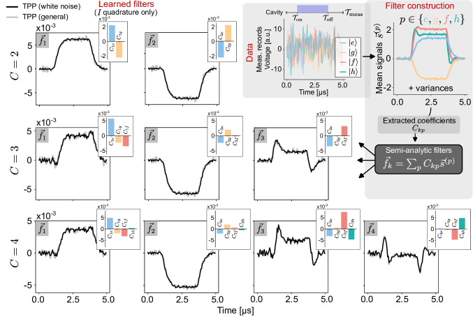
Figure 2: TPP-learned optimal filters for simulated multi-state classification under Gaussian white noise conditions. Top right: single-shot measurement records obtained under the indicated measurement tone, and empirical mean traces of several heterodyne records of the cavity $I$ quadrature corresponding to multi-level atom states $\ket{p}$ where $p\in\{e,g,f,h\}$. For a transmon $\chi_{p}/\kappa\in\{-\chi,\chi,-3\chi,-5\chi\}$, $\chi/\kappa=0.195$, and $\kappa/2\pi=1.54\leavevmode\nobreak\ {\rm MHz}$. Rows: TPP-learned optimal filters for classifying states $p\in\{e,g\}$ ($C=2$), $\{e,g,f\}$ ($C=3$), and $\{e,g,f,h\}$ ($C=4$). Black curves are filters learned under the white noise assumption, calculated analytically using Eq. (15). Bar plots show the coefficients $C_{kp}$ applied to respective mean traces in calculating these filters. Gray curves are general filters calculated by numerically solving Eq. (8). Both analytically-computed white noise filters and general filters can be extended to arbitrary $C$.

III.1 TPP learning mechanism and interpretation as optimal filtering

While Eq. (7) presents a formal mathematical formulation of the TPP framework in the machine learning context, we can develop further understanding of how the TPP learns from data to enable classification. To this end, we first note that this stochastic measurement data can be written in the very general form:

$$\bm{\vec{x}}^{(\sigma)}=\bm{\vec{s}}^{(\sigma)}+\bm{\vec{\zeta}}^{(\sigma)}$$ (9)

Here $\bm{\vec{\zeta}}^{(\sigma)}$ describes the stochasticity of the measured data: for heterodyne measurement, for example, this includes the noise sources from Eq. (3a), (3b), including quantum noise. We take the noise process to have zero mean, $\mathbb{E}[\bm{\vec{\zeta}}^{(\sigma)}_{j}]=0$. Then, $\bm{\vec{s}}^{(\sigma)}=\mathbb{E}[\bm{\vec{x}}^{(\sigma)}]$ are simply the mean traces of the measured data for state $\sigma$. Crucially, the noise is characterized by nontrivial second-order temporal correlations, which we define as $\bm{\Sigma}^{(\sigma)}_{jk}=\mathbb{E}[\bm{\vec{\zeta}}^{(\sigma)}_{j}\bm{\vec{\zeta}}^{(\sigma)}_{k}]$. Higher-order correlations of the noise will also be generally non-zero, but are not relevant for the discussion here.

The use of a least-squares cost function in Eq. (8) means that a closed form of the optimal weights $\mathbf{W}^{\rm opt}$ and biases $\mathbf{b}^{\rm opt}$ learned by the TPP can be obtained (see Appendix D). Furthermore, the form of Eq. (9) allows us to write these learned weights and biases as

$$\begin{pmatrix}\mathbf{W}^{\rm opt}&\mathbf{b}^{\rm opt}\end{pmatrix}=\mathbf{M}\mathbf{D}^{-1}.$$ (10)

Here $\mathbf{M}$ is a matrix that depends only on the mean traces (full form in Appendix D). In contrast, $\mathbf{D}$ is the matrix of second-order moments:

$$\mathbf{D}=\begin{pmatrix}\mathbf{G}+\mathbf{V}&\sum_{c}\bm{\vec{s}}^{(c)}\\ \sum_{c}(\bm{\vec{s}}^{(c)})^{T}&C\end{pmatrix}$$ (11)

which depends on the the “Gram” matrix of mean traces, $\mathbf{G}=\sum_{c}\bm{\vec{s}}^{(c)}(\bm{\vec{s}}^{(c)})^{T}$, but also on the temporal correlations via the matrix $\mathbf{V}=\sum_{c}\bm{\Sigma}^{(c)}$. Both these quantities emerge naturally in the analysis of the resolvable expressive capacity of noisy physical systems [40]. Here, Eq. (10) implies that weights learned by the TPP are not determined only by data means via $\mathbf{G}$, but are also sensitive to temporal correlations through $\mathbf{V}$. We will explore this dependence in the rest of our analysis.

Secondly, we find that the operation of TPP weights on data can be recast to clarify its connections to standard filtering-based classification schemes. To do so, we note that the learned matrix of weights $\mathbf{W}^{\rm opt}\in\mathbb{R}^{C\times N_{\rm O}\cdot N_{\rm T}}$ can be equivalently expressed as:

$$\mathbf{W}^{\rm opt}=\begin{pmatrix}\bm{\vec{f}}_{1}^{\leavevmode\nobreak\ T}\\ \vdots\\ \bm{\vec{f}}_{C}^{\leavevmode\nobreak\ T}\end{pmatrix}$$ (12)

where $\bm{\vec{f}}_{k}\in\mathbb{R}^{N_{\rm O}\cdot N_{\rm T}}$ for $k\in[C]$. With this parameterization, Eq. (7) for the $k$th component of the vector $\mathbf{y}$ can be rewritten as:

$$\mathbf{y}_{k}=\bm{\vec{f}}_{k}^{\leavevmode\nobreak\ T}\bm{\vec{x}}+\mathbf{b}_{k},\leavevmode\nobreak\ \leavevmode\nobreak\ \leavevmode\nobreak\ k\in[C]$$ (13)

When compared against Eq. (5), the interpretation of $\bm{\vec{f}}_{k}$ becomes clear: this set of weights can be viewed as a temporal filter applied to the data $\bm{\vec{x}}$. As a result, TPP based classification can equivalently be interpreted as the application of $C$ filters (one for each $k$) to obtain the estimated label $\sigma^{\rm est}$. The optimal $\mathbf{W}^{\rm opt}$ therefore defines the optimal filters that enable this estimation with minimal error. The use of $C$ optimal filters for a $C$-state classification task indicates the linear scaling of the TPP approach with the complexity of the task. Furthermore, we note that the $C$ filters are not all independent; they can be shown to satisfy the constraint (see Appendix D)

$$\sum_{k=1}^{C}\bm{\vec{f}}_{k}=\bm{\vec{0}},$$ (14)

where $\bm{\vec{0}}\in\mathbb{R}^{N_{\rm O}\cdot N_{\rm T}}$ is the null vector. This powerful constraint, which holds regardless of the statistics of the noise $\bm{\vec{\zeta}}$, implies that only $C-1$ of the $C$ filters need to be learned from training data.

III.2 TPP-learned optimal filters for multi-state classification under Gaussian white noise

We begin by analyzing the case most often considered in cQED measurement chains, where the dominant noise source in heterodyne records $I,Q$ is Gaussian white noise, which is assumed to be state and time-independent. Engineering of cQED measurement chains is geared towards approaching this limit, by (i) developing large bandwidth, high dynamic range amplifiers that operate with fast response times and minimal nonlinear effects even at high gain and large input signal powers [41, 42],[43, 44, 45, 46], (ii) improving qubit $T_{1}$ and tolerance to strong cavity drives to reduce transitions during $\mathcal{T}_{\rm meas}$ [3], and (iii) controlling technical noise sources such as electronic white noise from classical cryo-HEMT amplifiers and room temperature electronics.

In this relevant limit, we show that the $C$ filters defined in Eq. (13) can be computed via:

$$\bm{\vec{f}}_{k}=\sum_{p\in\{e,g,\ldots\}}\!\!\!\!C_{kp}\bm{\vec{s}}^{(p)},\leavevmode\nobreak\ \leavevmode\nobreak\ \leavevmode\nobreak\ k\in[C]$$ (15)

where $\bm{\vec{s}}^{(p)}$ are the empirically-calculated mean traces under the known initial state $p$:

$$\bm{\vec{s}}^{(p)}=\frac{1}{N_{\rm train}}\sum_{n=1}^{N_{\rm train}}\bm{\vec{x}}_{(n)}^{(p)}$$ (16)

while the coefficients $C_{kp}$ can also be shown to depend only on $\bm{\vec{s}}^{(p)}$ and additionally the variance of the measured heterodyne records, assumed to be observable-independent and time-invariant, as mentioned earlier. Formally, here the correlation matrix $\mathbf{V}$ becomes proportional to the identity matrix (see Appendix D for full details). The TPP-learned optimal filters in the Gaussian white noise approximation are therefore simply a semi-analytically calculable linear combination of the mean traces. As a result, obtaining these optimal filters only requires the calculation of an empirical mean of the measurement records for each state, and an empirical estimate of the variances.

We now present an example of TPP-learned optimal filters for dispersive qubit readout where the dominant noise source is additive Gaussian white noise. This is ensured via a theoretical simulation of Eq. (1) to generate a dataset of measured heterodyne records for $C$ qubit states, under the following assumptions: (i) all qubit state transitions are neglected, (ii) any additional classical noise sources in the measurement chain are ignored, and (iii) therefore direct readout of the cavity can be considered instead of the use of a quantum amplifier and the potential quantum noise added by it. We take the cavity measurement tone to be applied for a subset of the total $\mathcal{T}_{\rm meas}$, namely for $[\mathcal{T}_{\rm on},\mathcal{T}_{\rm off}]$ (see Fig. 2, top right), and to be coincident with the cavity center frequency so that $\Delta_{da}=0$, usual for transmon readout (for full details, see Appendix B.1). Other system parameters can be found in the caption of Fig. 2. We note that the specific details of the readout scheme do not change the TPP learning procedure. These simulations yield single-shot measurement records for any number of transmon states. Examples of these records are then shown in Fig. 2 for four distinct transmon states $p\in\{e,g,f,h\}$; for ease of visualization we only consider the $I$ quadrature.

We use this simulated dataset as a training set to determine the TPP-learned filters under the white noise assumption, as defined by Eq. (15). While the individual measurement records are obscured by white noise, the empirically-calculated mean traces in the top right of Fig. 2 illustrate the physics at play. The mean traces grow once the measurement tone is turned on past $\mathcal{T}_{\rm on}$, and settle to a steady state depending on the induced dispersive shift $\chi_{p}$ and the measurement amplitude. The traces begin to fall beyond $\mathcal{T}_{\rm off}$ and eventually settle to background levels. These means, together with an estimate of the variances, determine the coefficients $C_{kp}$ that define the contribution of the mean trace $\vec{s}^{(p)}$ to the $k$th filter, and are hence sufficient to calculate optimal filters for the classification of any subset of states.

For the standard binary classification task ($C=2$) of distinguishing $\{e,g\}$ states, the learned filters are shown in black in the top row of Fig. 2, together with bar plots showing the coefficients $C_{kp}$. Again for visualization, we only show filters $\vec{f}_{k}\in\mathbb{R}^{N_{\rm T}}$ for $I$ quadrature data; the complete vector $\bm{\vec{f}}_{k}$ includes filters for all $N_{\rm O}$ observables. For the binary case, the $k=1$ TPP-learned filter always satisfies $C_{1e}=-C_{1g}$. Hence it is simply proportional to the difference of mean traces for the two states, $\vec{f}_{1}\propto\vec{s}^{(e)}-\vec{s}^{(g)}$, making it exactly equivalent to the standard matched filter for binary classification (see Appendix D). We note that the second filter ($k=2$) is simply the negative of the first, as demanded by Eq. (14).

Crucially, the TPP approach now provides the generalization of such matched filters to the classification of an arbitrary number of states. For three-state ($C=3$) classification of $\{e,g,f\}$ states, the three TPP-learned filters are plotted in the middle row, while the last row shows the four filters for the classification of $C=4$ states $\{e,g,f,h\}$. Filters for the classification of an arbitrary number of states $C$ can be constructed similarly. The bar plots of $C_{kp}$ show how these filters typically have non-zero contributions from the mean traces for all states. This emphasizes that the TPP-learned filters are not simply a collection of binary matched filters, but a more non-trivial construction. Most importantly, our analytic approach enables this construction by inverting a matrix in $\mathbb{R}^{(C-1)\times(C-1)}$ to determine $C_{kp}$. This is a substantially lower complexity relative to the pseudoinverse calculation demanded by Eq. (8), which requires inverting a much larger matrix in $\mathbb{R}^{N_{\rm O}\cdot N_{\rm T}\times N_{\rm O}\cdot N_{\rm T}}$ (see Appendix D).

Of course, the latter approach of obtaining $\mathbf{W}^{\rm opt}$ and hence TPP filters using Eq. (8) can also be employed for learning using the same training data. Here, it yields the underlying filters in gray. The resulting filters appear to simply be noisier versions of the analytically calculated filters. The reason for this straightforward: the fact that the noise in the measurement data is additive Gaussian white noise is a key piece of information used in calculating the TPP filters via Eq. (15), but is not a priori known to the general RC. The latter makes no assumptions regarding the underlying noise statistics of the dataset. Instead, the training procedure itself enables the TPP to learn the statistics of the noise and adjust $\mathbf{W}^{\rm opt}$ accordingly. The fact that the general TPP filters approach the white noise filters shows this learning in practice. This ability to extract noise statistics from data is a key feature that makes TPP learning useful under more general noise conditions, as we will demonstrate in Secs. IV, V.

III.3 TPP performance under Gaussian white noise in comparison to standard FGDA

We now analyze the classification performance using TPP-learned optimal filters from the previous section in comparison to the standard FGDA approach. For concreteness, we perform dispersive qubit readout to distinguish $C=3$ states $p\in\{e,g,f\}$. Recall that we consider the measurement tone to be resonant with the cavity, as is often the case for transmon readout. Then, the sign of cavity dispersive shifts for transmon states $e$ and $f$ is the same, and is opposite to that for $g$, making them harder to distinguish (see also Fig. 3 inset).

For this three-state classification task, a unique filter choice for the FGDA is not known. While certain approaches at constructing filters have been attempted [47], boxcar filtering is still commonly employed. Another approach might be to use a matched filter that optimizes distinction of just one pair of states. There are 3 such filters in total: for discrimination of $e$-$g$ states as defined in Eq. (6), as well as analogously-defined filters for $e$-$f$ and $g$-$f$ states.

In Fig. 3, we show classification infidelities $1-\mathcal{F}$, calculated for datasets with increasing measurement tone amplitude (more opaque markers), using both the optimal TPP filter and the FGDA with the four aforementioned filter choices. We clearly observe that the FGDA infidelities for most choices are worse than the RC. Interestingly, the poorest performer is not the boxcar filter; instead, it is the $e$-$g$ filter, which would be optimal if we were only distinguishing $\{e,g\}$ states, that yields the worst performance. This is because the $e$-$g$ filter is completely unaware of the $f$ state: it attempts to best discriminate $e$ and $g$, but in doing so substantially confuses $e$ and $f$ states that are already the hardest to distinguish. The $e$-$f$ filter corrects this major problem and hence performs better, but does not discriminate $e$ and $g$ as well as the $e$-$g$ filter would. Due to the specific driving conditions and phases, the $g$-$f$ filter unwittingly does a good job at addressing both these problems, yielding the best performance. Nevertheless, it can only match the RC.

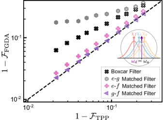
Figure 3: Multi-state ($C=3$) classification performance of TPP versus FGDA under Gaussian white noise conditions. We consider dispersive qubit readout to distinguish states $p\in\{e,g,f\}$ as a function of measurement power; more opaque markers indicate stronger measurement tone amplitudes. Inset shows induced dispersive shifts for each state (not to scale). Standard FGDA is performed using one of three MFs corresponding to each distinct state pair, as well as a boxcar filter. TPP filters are also followed by a Gaussian discriminator for an equivalent comparison. Only one of the binary MFs allows the FGDA to approach the TPP, while all other chosen filters yield a worse performance.

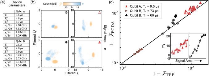
Figure 4: Classification performance of TPP versus FGDA for readout of real qubits. (a) Parameters of various dispersive qubit-cavity systems used for gathering readout data. Coherence measurements are subject to $10\%$ variation over time. (b) Representative qubit readout histograms under boxcar filtering as a function of measurement signal amplitude. (c) Readout data for three dispersive qubit-cavity systems is analyzed and the resulting classification infidelities for binary ($C=2$) state classification are plotted against each other. The dashed line marks $1-\mathcal{F}_{\rm FGDA}=1-\mathcal{F}_{\rm TPP{}}$. For datasets with variable shading of markers (red and black), more opaque markers indicate stronger measurement tone amplitudes. Inset: Percentage fewer errors $\mathcal{E}$ computed for indicated datasets with increasing input signal amplitude.

This trial-and-error approach relies on knowledge of optimal matched filtering from binary classification, but clearly cannot be optimal for $C>2$: none of the filter choices are informed by the statistical properties of measured data for all $C$ classes to be distinguished. Furthermore, the number of distinct state pairs, and hence pairwise matched filters, grows quadratically with $C$ in the absence of symmetries, making this brute force approach even less feasible for larger classification tasks. In contrast, the TPP approach provides a simple scheme to learn optimal filters that is automated, takes data for readout of all classes into account, and still scales linearly with the task dimension set by $C$.

However, the true strength of TPP learning arises when noise in measured heterodyne records no longer satisfies the additive Gaussian white noise assumption, which may arise if any of the conditions (i)-(iii) for qubit measurement chains listed in Sec. III.2 are not met. Departures from this ideal scenario are widely prevalent in cQED. Through the rest of this paper, we show how the trainability of the TPP approach enables it to learn filters tailored to these more general noise conditions, and consequently outperform the standard FGDA based on binary matched filters.

IV TPP-Learning for real qubits

IV.1 Experimental Results

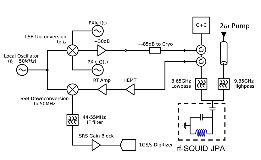
Figure 9: Upconversion and downconversion schematic for drive pulses sent first to the qubit readout resonator, driven in reflection, then routed to the amplifier and to the HEMT via two circulators.

To demonstrate how the general learning capabilities of the TPP approach can aid qubit state classification in a practical setting, we now apply it to the readout of finite-lifetime qubits in an experimental cQED measurement chain. The essential components of the measurement chain are as depicted schematically in Fig.  1 and described by Eq. (1). The actual circuit diagram is shown in Fig. 9 in Appendix A, and important parameters characterizing the measurement chain components are summarized in Fig. 4(a).

We consider two distinct cavity systems, for the dispersive readout of distinct single qubits A and B to discriminate states $p\in\{e,g\}$. For lossless qubits that are read out dispersively for a fixed measurement time $\mathcal{T}_{\rm meas}$, the ratio $\chi/\kappa$ determines the theoretical maximum readout fidelity; in particular, an optimal value for this ratio is known under these ideal conditions [32]. However, experimental considerations mean that operating parameters must be designed with several other factors in mind. At high $\chi/\kappa$ ratios with modest or higher $\kappa$, for large $\kappa$ with modest $\chi/\kappa$ ratios, and especially when both are true, the experiment is sensitive to dephasing from the thermal occupation of the readout resonator at a rate proportional to $\bar{n}\kappa$ [48]. This can be quite limiting to the $T_{2}$ dephasing time of the qubit if the readout resonator is strongly coupled to the environment and/or the environment has appreciable average thermal photon occupation $\bar{n}$. In the opposite low $\chi/\kappa$ limit, the qubit is shielded from thermal dephasing, but readout becomes very difficult as the rate at which one learns about the qubit state from a steady state coherent drive is proportional to $\chi/\kappa$ [32]. In this experiment, the lower-than-usual $\chi/\kappa\approx 0.2$ in qubit B represents a compromise between these two limits, while also enabling the high fidelity discrimination of multiple excited states of the transmon (See Fig. A8).

Each readout cavity is driven in reflection, and its output signal is amplified also in reflection using a Josephson Parametric Amplifier (JPA). We employ the latest iteration of strongly-pumped and weakly-nonlinear JPAs [46], boasting a superior dynamic range. Such JPAs operate well below saturation even at signal powers that correspond to over 100 photons, enabling us to probe qubit readout at high measurement powers. By choosing a signal frequency at exactly half the pump frequency, we can operate the JPA in phase-sensitive mode. We can also operate the amplifier in phase-preserving mode if we detune the signal from half the pump frequency by greater than the spectral width of the pulse. Several filters are used to reject the strong JPA pump tone required to enable this operation. Circulators are used to route the output signals away from the input signals and to isolate the qubit from amplified noise.

In principle, the use of these stronger measurement tones should enhance the classification fidelity for qubit readout. In practice, however, higher measurement powers are known to be associated with a variety of complex dynamical effects. Perhaps the most common observation is enhanced qubit $e\to g$ decay under strong driving (referred to as the $T_{1}$ versus $\bar{n}$ problem). The relative accessibility of higher excited states in transmon qubits means that at strong enough driving, general multi-level transitions to these higher levels can also be observed. There have also been predictions of chaotic dynamics and ionization  [49, 14] at certain readout resonator occupation levels. The theoretical understanding of these effects, and their modeling via an SME analogous to Eq. (1) is an ongoing challenge.

In our experiments, we perform readout across this domain using measurement pulse durations ($\mathcal{T}_{\rm off}-\mathcal{T}_{\rm on}$) ranging from 500 ns to 900 ns, and measurement amplitudes from 0.04 to 0.09 in arbitrary voltage units, corresponding to roughly 44 to 100 photons in the cavity in the steady state. At the lowest pulse duration and amplitude, this corresponds to just enough discriminating power to separate the measured distributions for the two states by approximately their width in a boxcar-filtered IQ plane (namely, without the use of an empirical MF). An example of the individual readout histograms for qubits initialized in states $p\in\{e,g\}$ at this lowest measurement tone power is shown in Fig. 4(a).

At the highest measurement powers, we are able to populate the readout cavity with up to 100 photons, calibrated by observing the frequency shift of the qubit drive frequency versus the occupation of the readout resonator. At these powers, extreme higher-state transitions become visible during the readout pulse [9]; an example is shown in Fig. 4(a) (see also Fig. 8 in Appendix A). There is also a notable elliptical distortion in the high-amplitude data, particularly for qubit A. We suspect that this is due to the short duration of the pulses and the inclusion of the cavity ring-up and ring-down in the integration, since the simple boxcar filter used to integrate the histograms in Fig. 4 does not rotate with the signal mean.

For such complex regimes where no simple model of the dynamics exists, the construction of an optimal filter is not known; this hence serves as an ideal testing ground for the TPP approach to qubit state classification. We compute the infidelities of binary classification using both the TPP scheme and an FGDA using the standard MF [Eq. (6)] under a variety of readout conditions, plotting the results against each other in Fig. 4.

The highest fidelity using both schemes is obtained for qubit B under conditions where its $T_{1}$ time is longest. This dataset was collected at a fixed, moderate measurement power; the different points correspond to a rolling of the relative JPA pump and measurement tone phase that determines the amplified quadrature under phase-sensitive operation. The dashed line marks equal classification infidelities, so that any datasets above this line yield a higher classification infidelity with the FGDA than with the RC. Here we see that both schemes exhibit very similar performance levels.

The other two datasets are obtained for readout under varying measurement powers. The depth of shading of the markers indicates the strength of measurement drives: the more opaque the marker, the stronger the measurement power. For weaker measurement powers, we see that the TPP and the FGDA are once again comparable. However, a very clear trend emerges: for stronger measurement powers - where measurement dynamics become much more complex as demonstrated in Fig. 4(a) - the TPP generally outperforms the FGDA.

To more precisely quantify the difference in performance between the TPP and FGDA, we introduce the metric $\mathcal{E}$:

$$\mathcal{E}=\left(\frac{\mathcal{F}_{\rm TPP{}}-\mathcal{F}_{\rm FGDA}}{1-\mathcal{F}_{\rm FGDA}}\right)\!\times\!100$$ (17)

which essentially asks: “what percentage fewer errors does the TPP make when compared to the FGDA?” We plot $\mathcal{E}$ in the inset of Fig. 4 for the two qubit readout experiments where the input signal amplitude is varied. We see clearly that with increasing amplitude, the TPP can significantly outperform the FGDA scheme, committing as many as 30% fewer errors in the experiments considered.

Our results demonstrate that the TPP approach can be successfully applied to real qubit readout across a broad spectrum of measurement conditions. Furthermore, the TPP can even outperform the standard FGDA in certain relevant regimes, such as for high-power readout. While the TPP can thus be applied as a model-free learning tool, we are also interested in understanding the principles that enable the TPP to outperform standard approaches using an MF. Uncovering these principles can help identify the types of classification tasks where TPP learning is essential. Our interpretation of TPP learning as optimal filtering proves a useful tool in this vein.

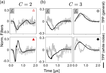
Figure 5: Adaptation of TPP-learned filters with increasing measurement tone amplitude and evolving noise conditions. Black curves are normalized TPP filters under the white noise assumption; for binary state classification, these are identical to standard matched filters. Gray curves are general TPP filters with no assumptions on noise statistics. (a) Filter $\vec{f}_{1}$ for binary ($C=2$) classification, and (b) filters $\vec{f}_{1,3}$ for $C=3$ state classification. In both cases, at weaker amplitudes the general TPP filter closely matches the TPP filter assuming white noise. However, for stronger measurement amplitudes, a marked difference between the white noise TPP filter and the general TPP filter is observed.

IV.2 Adaptation of TPP-learned filters under strong measurement tones

The observed difference in performance between the TPP and the standard FGDA lies in the former’s ability to learn from data as experimental conditions evolve. Our interpretation of TPP learning as the determination of optimal filters proves particularly insightful in expressing this adaptability.

Recall that for a $C$ state classification task, the TPP learns $C$ filters; however, the sum of filters is constrained by Eq. (14), so that $C-1$ filters are sufficient to describe the TPP’s learning capabilities. In Fig. 5(a) we first consider filters learned by the TPP for a $C=2$ classification task, for select experimental datasets from Fig. 4 obtained under a low and a high measurement power. It therefore suffices to analyze just $\vec{f}_{1}$, the first filter for the $I$ quadrature, as a function of measurement power. The black curves are filters learned under the assumption of Gaussian white noise, given by Eq. (15); recall that for this binary case, these filters are exactly the standard MF. The gray curves, in contrast, are filters learned by the TPP for arbitrary noise conditions, obtained by solving Eq. (8). At a low measurement tone amplitude (less opaque marker), the general TPP filter appears very similar to the TPP filter under white noise. As the measurement tone amplitude is increased, however, the TPP-learned filter under arbitrary noise can deviate substantially from the TPP filter under white noise. This is accompanied by a marked difference in performance, as observed earlier.

Crucially, the generalization of matched filters provided by TPP-learning via Eq. (15) enables a similar comparison for classification tasks of an arbitrary number of states. We show learned filters for $C=3$ state classification of $p\in\{e,g,f\}$ in Fig. 5(b), again for a low and high measurement power. It is now sufficient to consider any two of three distinct $I$-quadrature filters; here we choose $\vec{f}_{1}$ and $\vec{f}_{3}$. Once more, the general TPP filters begin to deviate significantly from TPP filters under the white noise assumption at high powers.

Clearly, the precise form of filters learned by the TPP to outperform white noise filters must be influenced by some physical phenomena that arise at strong measurement powers. However, the TPP is not provided with any physical description for such phenomena, which is in fact part of its model-free appeal. What then, is the mechanism through which the TPP can learn about such phenomena to compute optimal filters? The answer lies in Eq. (10): TPP-learned filters are sensitive to noise correlations in data via $\mathbf{V}$. Using simulations of measurement chains where the noise structure of quantum measurement data can be precisely controlled, we show that the noise structure can strongly deviate from white noise conditions under practical settings.

V TPP learning: Simulation results

V.1 Learning correlations

As discussed in Sec. III.1, the learned weights and hence optimal filters depend on mean traces, but are also cognizant of - and can learn from - the noise structure of measured data via the temporal correlation matrix $\mathbf{V}$. This is in stark contrast to the use of a matched filter.

Crucially, when learning from data obtained from quantum systems, the observed correlations can have a quantum-mechanical origin. In what follows, we demonstrate the ability of the TPP to learn these quantum correlations, using simulations of two experimental setups where such quantum noise sources arise naturally: (i) readout using phase-preserving quantum amplifiers with a finite bandwidth, so that the amplifier added noise (demanded by quantum mechanics) has a nonzero correlation time, and (ii) readout of finite lifetime qubits with multi-level transitions (quantum jumps).

V.2 Correlated quantum noise added by finite-bandwidth phase-preserving quantum amplifiers

Quantum-limited amplifiers are a mainstay of measurement chains in cQED, needed to overcome the added classical noise of following HEMTs. Phase-preserving quantum amplifiers are necessitated by quantum mechanics to add a minimum amount of noise to the incoming cavity signal being processed. The correlation time of this added quantum noise is determined by the dynamics of the amplifier itself, namely its active linewidth reduced by anti-damping necessary for gain. For finite bandwidth amplifiers operating at large enough gains, this can lead to the addition of quantum noise with non-zero correlation time in measured heterodyne data.

To simulate qubit readout in these circumstances, we consider a quantum measurement chain described by Eq. (1) now consisting of a qubit-cavity-amplifier setup. $\mathcal{L}_{\rm meas}$ then describes the readout of a non-degenerate (i.e. two-mode) parametric amplifier and its non-reciprocal coupling to the cavity used to monitor the qubit. We ignore qubit state transitions, so that $\mathcal{L}_{\rm envt}$ only describes losses via unmonitored ports of the cavity and amplifier. Full details of the simulated SME are included in Appendix B.2.

We must consider added classical noise in the measurement chain, as this is what demands the use of a quantum amplifier in the first place. We take the added classical noise to be purely white, $\xi^{\rm cl}(t_{i})=\sqrt{\bar{n}_{\rm cl}}\frac{dW}{dt}(t_{i})$, with a noise power $\bar{n}_{\rm cl}=30$, parameterized as usual in “photon number” units; these assumptions on the noise structure and power are taken from standard cQED experiments, including our own. Now, the obtained heterodyne measurement records, Eqs. (3a), (3b) contain two dominant noise sources: (i) excess classical white noise, and (ii) quantum noise added by the amplifier, contained once again in quantum trajectories $\langle\hat{X}^{(\sigma)}(t)\rangle_{c}$ and $\langle\hat{P}^{(\sigma)}(t)\rangle_{c}$.

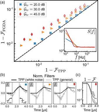
Figure 6: Classification performance of TPP versus FGDA on simulated dataset of readout via a phase-preserving quantum amplifier. (a) Classification infidelities for varying amplifier transmission gains $\mathcal{G}_{\rm tr}$ as a function of measurement signal amplitude (more opaque markers are higher amplitudes). The ratio of the bare amplifier linewidth to the cavity mode linewidth is $\gamma/\kappa=5$. Noise PSD is shown in the inset for the different operating gains (for a linear amplifier, this is independent of the measurement signal amplitude). (b) Learned filters under white noise assumption (black) and general noise conditions (gray) for representative datasets of each value of $\mathcal{G}_{\rm tr}$. (c) Classification infidelities as a function of total time $t$. The measurement tone is only on between the two vertical dashed lines.

We restrict ourselves for the moment to binary classification of states $\ket{e}$ and $\ket{g}$; here, the matched filtering (MF) scheme is unambiguously defined, and serves as a concrete benchmark for comparison to the TPP approach. In Fig. 6, we compare calculated infidelities using the FGDA and TPP approaches for three different values of amplifier transmission gain $\mathcal{G}_{\rm tr}$, and as a function of the coherent input tone power: darker markers correspond to readout with stronger input tones.

To understand how correlations in the measured data depend on the varying amplifier gain, we introduce the noise power spectral density (PSD) of the data (here, the $I$-quadrature) for state $\ket{p}$,

$$S^{(p)}[f]\approx\sum_{j>k}^{N_{\rm T}}e^{-i2\pi f\tau_{jk}}\bm{\Sigma}_{jk}^{(p)}$$ (18)

where $\tau_{jk}=\Delta t(j-k)$. The PSD is simply the Fourier transform of the noise autocorrelation function (by the Wiener-Khinchin theorem). Through $\mathbf{V}$, the TPP learns from these correlations when optimizing filters. The noise PSD is plotted in the inset of Fig. 6; for the current readout task, this is independent of $p$. With increasing gain, the PSD deviates from the flat spectrum representative of white noise to a spectrum peaked at low frequencies, indicative of an extended correlation time. The observations also emphasize that added noise by the quantum amplifier dominates over heterodyne measurement noise $\xi$, as well as excess classical noise $\xi^{\rm cl}$.

For the lowest considered amplifier gain, we see that the FGDA and TPP classification performance is quite close. However, with increasing gain, the FGDA infidelity is substantially higher, up to an order of magnitude worse for the largest gain considered here. This TPP performance advantage is enabled by optimized filters, shown in Fig. 6(b). The measurement tone is only on between the two dashed vertical lines. The curves in black show white noise filters, exactly equal to the MF in this binary case. Note that these filters also change with gain: the amplifier response time increases at higher gains, so the mean traces and hence the MF derived from these traces exhibit much slower rise and fall times. The general TPP filter is similar to the MF at low gains, but becomes markedly distinct at higher gains.

Interestingly, one such change is that at high gains the general TPP filter becomes non-zero even prior to the measurement signal turning on (the first vertical dashed line). This appears odd at first sight, since there must not be any information that could enable state classification before a measurement tone probes the cavity used for dispersive qubit measurement. To validate this, in Fig. 6(d) we plot $1-\mathcal{F}$ calculated for an increasing length of measured data, $t\in[0,\mathcal{T}_{\rm meas}]$. We clearly see that for $t<\mathcal{T}_{\rm on}$, both the TPP and FGDA cannot distinguish the states, as must be the case. The non-zero segment of the general TPP filter before $\mathcal{T}_{\rm on}$ instead accounts for noise correlations. In particular, due to the long correlation time of noise added by the quantum amplifier, noise in data beyond $\mathcal{T}_{\rm on}$ is correlated with noise from $t<\mathcal{T}_{\rm on}$. The general TPP filter is aware of these correlations that the standard MF is completely oblivious to, and by accounting for them improves classification performance.

V.3 Correlated quantum noise due to multi-level transitions

A transmon is a multi-level artificial atom, as described by Eq. (2); as a result, it is possible to excite levels beyond the typical two-level computational subspace of $e$ and $g$ states. Such transitions manifest as stochastic quantum jumps in quantum measurement data, and are an important source of error in readout.

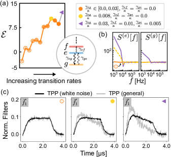
Figure 7: Classification performance of TPP versus FGDA on simulated dataset of readout of a qubit experiencing multi-level transitions. (a) $\mathcal{E}$ as a function of increasing transition rate values (more opaque markers), as shown. Schematic in the inset shows transmon levels and non-zero transition rates considered. (b) Noise PSD $S^{(p)}[f]$ for three representative datasets in the inset, indicating deviation from flat (white noise) as measurement data includes more transitions. (c) TPP learned filters (gray) compared to matched filters (black) for representative datasets, showing adaptation with transition rates.

To model measurement under such conditions, we now consider the dispersive heterodyne readout of a finite lifetime transmon with possible occupied levels $\{e,g,f\}$. We further allow only a subset of all possible allowed transitions between these levels, and with static rates: $\ket{e}\to\ket{g}$ at rate $\gamma_{eg}$, the reverse $\ket{g}\to\ket{e}$ at rate $\gamma_{ge}$, and $\ket{e}\to\ket{f}$ at rate $\gamma_{ef}$ (see Fig. 7 inset). The transitions are described by superoperator $\mathcal{L}_{\rm envt}$, while $\mathcal{L}_{\rm meas}$ describes the measurement tone incident on the cavity, and the heterodyne measurement superoperator for the same; for full details see Appendix B.3.

For simplicity, we now further neglect excess classical noise added by the measurement chain, dropping terms $\xi_{I/Q}^{\rm cl}(t)$. As a result, the obtained measurement records, Eqs. (3a), (3b), contain only two noise sources: white heterodyne measurement noise, and quantum noise due to qubit state transitions imprinted on the emanated cavity field, contained in quantum trajectories of cavity quadratures $\langle\hat{X}^{(\sigma)}(t)\rangle_{c}$ and $\langle\hat{P}^{(\sigma)}(t)\rangle_{c}$. We then generate simulated datasets by integrating the resulting full SME, Eq. (1) for different values of transition rates, and consider the task of binary classification of states $p\in\{e,g\}$.

We compare the performance of a trained TPP against that of an FGDA with an empirical MF using the metric $\mathcal{E}$ in Fig. 7(a) with varying transition rates. The noise PSD is plotted in Fig. 7(b) for representative datasets. In the absence of any transitions (lightest orange), $S^{(p)}[f]$ is flat at all frequencies, regardless of the initially prepared state $p$. This is because the measured data only has heterodyne white noise. With an increase in $\gamma_{eg}$, we note that $S^{(e)}[f]$ deviates from the white noise spectrum, attaining a peak at low frequencies. In contrast, $S^{(g)}[f]$ remains unchanged as trajectories for initial states $\ket{g}$ undergo no transitions. In the most complex case where we allow for all considered transitions, $S^{(g)}[f]$ also starts to demonstrate deviation from the white noise spectrum.

From readout datasets with no transitions to readout data with increasing transition rates, we note a small but clear improvement in classification performance using the trained TPP in comparison to the FGDA. That the TPP is able to learn information in the presence of transitions that evades the MF is clear when we compare the two sets of filters in Fig. 7(c). As the transition rates increase, the MF undergoes modifications due to the changes to the means of heterodyne records. However, the TPP is sensitive to changed beyond means - in the correlations of measured data - and increasingly learns a distinct filter with sharply decaying features. We note that the utility of similar exponential linear filters for finite-lifetime qubits has been the subject of earlier analytic work [19]. The TPP approach generalizes the ability to learn such filters in the presence of arbitrary transition rates and measurement tones, and for multi-state classification.

We emphasize that the simplified transition model considered here is chosen to highlight the ability of the TPP to learn quantum noise associated with quantum jumps under controlled noise conditions, where no other nontrivial noise sources (classical or quantum) exist. The TPP approach to learning is model-free, and its ability to learn in more general noise settings is demonstrated by its adaptation to real qubit readout in Sec. IV.

VI Discussion and Outlook

In this paper we have demonstrated a reservoir computing approach to classification of an arbitrary number of states using temporal data obtained from quantum measurement chains. While we have focused on the task of dispersive readout of multi-level transmons, the TPP approach applies broadly to quantum systems, and more generally physical systems, monitored over time. Our results show that the TPP framework for processing quantum measurement data reduces to standard approaches based on matched filtering in the precise regimes of validity of the latter. However, the TPP can adapt to more general readout scenarios to significantly outperform matched filtering schemes. We show this improvement for RCs trained on real qubit readout data to confirm the practical utility of our scheme.

Rather than treating the TPP as a black box, in our work we clarify the learning mechanism that enables the TPP to outperform matched filtering schemes. First, we develop a heuristic interpretation of the TPP mapping as one of applying temporal filters to measured data. TPP learning then amounts to learning optimal filters. Deconstructing the learning scheme, we find the TPP performance advantage is enabled by its ability to learn optimal filters by accounting for noise correlations in temporal data. When this noise is purely white, the TPP approach provides a generalization of matched filtering to an arbitrary number of states.

Crucially, we find that the TPP can efficiently learn from correlations not just due to classical signals, or in principle due to quantum noise in theory, but from practical systems where the majority of the noise is quantum in origin. In addition to real qubit readout, using theoretical simulations where the strength of quantum noise sources can be tuned precisely, such as noise due to multi-level transitions or the added noise of phase-preserving quantum amplifiers, we clearly demonstrate that the TPP can learn from quantum noise correlations to outperform standard matched filtering.

The TPP approach, anchored by its connection to standard matched filtering under simplified readout conditions, with demonstrated advantages for real qubit readout under more complex readout conditions, and feasible for FPGA implementations (to be demonstrated in future work), is ideal for integration with cQED measurement chains for the next step in readout optimization. Furthermore, the TPP’s generality and ability to learn from data could pave the way for an even broader class of applications. An important potential use is as a post-processor of quantum measurement data for quantum machine learning. With the use of general quantum machines for information processing, the optimal means to extract data from their measurements may not always be known. The TPP is ideally suited to uncover the optimal post-processing step, through training that could be incorporated parallel to, or as part of, the optimization of the quantum machine. Finally, optimal state estimation is essential for control applications. The trainable TPP can form part of a framework for control applications, such as Kalman filtering for quantum systems.

[appendices] [appendices]l1

Appendices

Appendix A Experimental Setup

In this appendix section, we show a few more examples of readout IQ histograms as well as a more detailed circuit diagram for the measurement chain. Shown in Fig. 8 below, we see two examples of the extremes of the measurement data used to generate Fig.4. Part (a) shows a lower power readout pulse performed for a short 300ns time, where the cavity barely has time to reach a steady state before the drive is turned off. Consequently, information from both the ring up and ring down must be integrated to achieve the SNR shown in this figure. Despite this measure, there is still significant infidelity from the lack of separation of the gaussian signals. In the second case, the displacement voltage is larger, and the pulse is three times as long, resulting in significantly increased separation of the gaussian signals and enabling discrimination of the $\ket{g},\ket{e},\ket{f}$ and $\ket{h}$ states. However, the large powers required induce transitions between these states, resulting in the trails between them as the measurement integrates a mixture of different cavity states at different times.

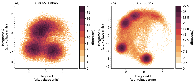
Figure 8: Comparison between boxcar-integrated IQ results of (a) a lower power pulse applied for a short time and (b) a higher power pulse applied for a longer time. State transitions are visible as "trails" leading between the primary symbols in (b). Counts are shown in logarithmic units to emphasize low-count trails.

In Fig. A9, the hardware schematic of the measurements in section IV are shown. The measurement setup is fairly standard, using single sideband upconversion to send signals into the dilution refrigerator, moving through three stages of attenuation with 20dB attenuation at 4K, 20dB attenuation at the 100mK stage, and approximately 45dB of attenuation at the base stage of the refrigerator, with 10dB of the base stage attenuation coming from a particularly well-thermalized copper body attenuator. The signal interacts with the qubit and cavity system, is routed by two circulation stages to the amplifier, amplified in reflection, and then is routed once again back through the circulators to the remaining stages of amplification at 4K and room temperature accordingly. From there it is downconverted by the same local oscillator to 50MHz, filtered, amplified once more at low frequency, digitized at 1GS/s, and finally demodulated and integrated to acquire a readout histogram such as the ones shown in Fig. 8.

Appendix B Simulating heterodyne measurement records obtained from quantum measurement chains for dispersive qubit readout

In this appendix section, we describe the SMEs used to model various quantum measurement chains and generated datasets analyzed in the main text. For convenience we reproduce the general SME of Eq. (1):

$$d\hat{\rho}_{c}=\mathcal{L}_{\rm sys}\hat{\rho}_{c}\leavevmode\nobreak\ dt+\mathcal{L}_{\rm envt}\hat{\rho}_{c}+\mathcal{L}_{\rm meas}[dW]\hat{\rho}_{c}$$ (19)

For all the considered models of quantum measurement chains for the fixed task of dispersive qubit readout, $\mathcal{L}_{\rm sys}$ remains the same, as identified in the main text:

$$\mathcal{L}_{\rm sys}\hat{\rho}_{c}=-i[\hat{\mathcal{H}}_{\rm disp},\hat{\rho}_{c}]$$ (20)

where $\hat{\mathcal{H}}_{\rm disp}$ is the dispersive cQED Hamiltonian for a multi-level artificial atom,

$$\hat{\mathcal{H}}_{\rm disp}\simeq\sum_{p}\omega_{p}|p\rangle\!\langle p|-\Delta_{da}\hat{a}^{\dagger}\hat{a}+\sum_{p}\chi_{p}\hat{a}^{\dagger}\hat{a}|p\rangle\!\langle p|$$ (21)

The superoperators $\mathcal{L}_{\rm envt}$ and $\mathcal{L}_{\rm meas}[dW]$ will depend on the specific model considered.

B.1 Dispersive readout with no qubit transitions and using a cavity

For qubit readout in the absence of any state transitions, $\mathcal{L}_{\rm envt}\to 0$. As a result, the SME of Eq. (19) takes the simpler form:

$$d\hat{\rho}_{c}=\mathcal{L}_{\rm sys}\hat{\rho}_{c}\leavevmode\nobreak\ dt+\mathcal{L}_{\rm meas}[dW]\hat{\rho}_{c}$$ (22)

Here $\mathcal{L}_{\rm sys}$ is given by Eq. (20). The superoperator $\mathcal{L}_{\rm meas}$ describes quantum modes in the measurement chain that are used to measure the quantum system of interest. This superoperator can be expressed in the general form:

$$\mathcal{L}_{\rm meas}[dW]\hat{\rho}_{c}=\mathcal{L}_{\rm q}\hat{\rho}_{c}+\mathcal{S}[dW]\hat{\rho}_{c}$$ (23)

Here $\mathcal{L}_{\rm q}$ defines the unconditional dynamics of quantum modes used for measurement; here, it takes the explicit form:

$$\mathcal{L}_{\rm q}\hat{\rho}=-i[\eta(\hat{a}+\hat{a}^{\dagger}),\hat{\rho}]+\kappa\mathcal{D}[\hat{a}]\hat{\rho}$$ (24)

which describes the measurement tone used for cavity readout, and the cavity losses due to its monitored port. Importantly, $\mathcal{L}_{\rm q}$ is independent of the qubit sector.

Then, $\mathcal{S}[dW]$ is the stochastic measurement superoperator that describes conditional evolution under continuous heterodyne monitoring:

$$\mathcal{S}[dW]\hat{\rho}_{c}=\sqrt{\frac{\kappa}{2}}\left(\hat{a}\hat{\rho}_{c}+\hat{\rho}_{c}\hat{a}^{\dagger}-\langle\hat{a}+\hat{a}^{\dagger}\rangle\hat{\rho}_{c}\right)dW_{I}+\sqrt{\frac{\kappa}{2}}\left(-i\hat{a}\hat{\rho}_{c}+i\hat{\rho}_{c}\hat{a}^{\dagger}-\langle-i\hat{a}+i\hat{a}^{\dagger}\rangle\hat{\rho}_{c}\right)dW_{Q}$$ (25)

These explicit forms of superoperators fully define Eq. (19) in this regime without qubit transitions. However, this assumption can be used to further simplify the form of the SME. In particular, in the absence of transitions, the quantum state of the measurement chain is given by the ansatz:

$$\hat{\rho}(t)=|p\rangle\!\langle p|\otimes\hat{\varrho}_{c}(t)$$ (26)

where $\hat{\varrho}_{c}(t)$ is the conditional density matrix defining the quantum state of all quantum modes in the measurement chain other than the qubit (namely, the cavity mode). The above implies that the qubit state is completely unchanged during the readout time. The only evolution is in the state of the modes used to readout the qubit, namely the cavity modes.

By now tracing out the qubit subspace in Eq. (19), we can obtain an SME for $\hat{\varrho}_{c}(t)$ alone, under the ansatz of Eq. (26). The Hamiltonian contribution from the dispersive qubit Hamiltonian yields:

$${\rm tr}_{Q}\{\hat{\mathcal{H}}_{\rm disp}|p\rangle\!\langle p|\otimes\hat{\varrho}_{c}\} ={\rm tr}_{Q}\Big{\{}\sum_{j}\omega_{j}\ket{j}\!\langle j|p\rangle\!\bra{p}\otimes\hat{\varrho}_{c}\Big{\}}-{\rm tr}_{Q}\Big{\{}|p\rangle\!\langle p|\otimes(\Delta_{da}\hat{a}^{\dagger}\hat{a}\hat{\varrho}_{c})\Big{\}}+{\rm tr}_{Q}\Big{\{}\sum_{j}\chi_{j}\hat{a}^{\dagger}\hat{a}\ket{j}\!\underbrace{\langle j|p\rangle}_{\delta_{jp}}\!\bra{p}\otimes\hat{\varrho}_{c}\Big{\}}$$

$$=\omega_{p}\hat{\varrho}_{c}-\Delta_{da}\hat{a}^{\dagger}\hat{a}\hat{\varrho}_{c}+\chi_{p}\hat{a}^{\dagger}\hat{a}\hat{\varrho}_{c}$$ (27)

and by conjugation,

$${\rm tr}_{Q}\{|p\rangle\!\langle p|\otimes\hat{\varrho}_{c}\hat{\mathcal{H}}_{\rm disp}\} =\hat{\varrho}_{c}\omega_{p}-\hat{\varrho}_{c}\Delta_{da}\hat{a}^{\dagger}\hat{a}+\hat{\varrho}_{c}\chi_{p}\hat{a}^{\dagger}\hat{a}$$ (28)

following which we arrive at:

$${\rm tr}_{Q}\{-i[\hat{\mathcal{H}}_{\rm disp},\hat{\rho}_{c}]\}=-i\left([-\Delta_{da}\hat{a}^{\dagger}\hat{a},\hat{\varrho}_{c}]+[\chi_{p}\hat{a}^{\dagger}\hat{a},\hat{\varrho}_{c}]\right)=-i[\left(-\Delta_{da}+\chi_{p}\right)\hat{a}^{\dagger}\hat{a},\hat{\varrho}_{c}]\equiv-i[\hat{\mathcal{H}}_{\rm cav},\hat{\varrho}_{c}]$$ (29)

where we have defined $\hat{\mathcal{H}}_{\rm cav}$ as the cavity Hamiltonian alone:

$$\hat{\mathcal{H}}_{\rm cav}=\left(-\Delta_{da}+\chi_{p}\right)\hat{a}^{\dagger}\hat{a}=(\omega_{a}+\chi_{p}-\omega_{d})\hat{a}^{\dagger}\hat{a}$$ (30)

We can perform a similar simplification on terms due to $\mathcal{L}_{\rm meas}$. For the ansatz in Eq. (26), we find for $\mathcal{L}_{\rm q}$:

$${\rm tr}_{Q}\{\mathcal{L}_{\rm q}(|p\rangle\!\langle p|\otimes\hat{\varrho}_{c})\} ={\rm tr}_{Q}\{|p\rangle\!\langle p|\otimes\mathcal{L}_{\rm q}\hat{\varrho}_{c}\}={\rm tr}_{Q}\{|p\rangle\!\langle p|\}\otimes\mathcal{L}_{\rm q}\hat{\varrho}_{c}=\mathcal{L}_{\rm q}\hat{\varrho}_{c}$$ (31)

As $\mathcal{L}_{\rm q}$ was independent of the qubit subsector, it remains unchanged following the partial trace over this subsector. The stochastic measurement operator $\mathcal{S}[dW]$ is again independent of the qubit subspace. Hence tracing out the qubit sector yields:

$$\sqrt{\kappa}\leavevmode\nobreak\ {\rm tr}_{Q}\{\mathcal{S}[dW]|p\rangle\!\langle p|\otimes\hat{\varrho}_{c}\}=\sqrt{\kappa}\leavevmode\nobreak\ {\rm tr}_{Q}\{|p\rangle\!\langle p|\}\otimes\mathcal{S}[dW]\hat{\varrho}_{c}=\sqrt{\kappa}\mathcal{S}[dW]\hat{\varrho}_{c}$$ (32)

The final cavity-only SME in the absence of any qubit transitions takes the form:

$$d\hat{\varrho}_{c}=-i[\hat{\mathcal{H}}_{\rm cav},\hat{\varrho}_{c}]dt+\mathcal{L}_{\rm meas}[dW]\hat{\varrho}_{c}$$ (33)

The resulting SME is purely linear and can be solved exactly using a truncated equations of motion (TEOMs) approach.

B.2 Dispersive readout with no qubit transitions and using a quantum-limited amplifier with added noise

As in the previous subsection, in the absence of any state transitions, $\mathcal{L}_{\rm envt}\to 0$, and the SME of Eq. (19) takes the simpler form:

$$d\hat{\rho}_{c}=\mathcal{L}_{\rm sys}\hat{\rho}_{c}\leavevmode\nobreak\ dt+\mathcal{L}_{\rm meas}[dW]\hat{\rho}_{c}$$ (34)

Again $\mathcal{L}_{\rm sys}$ is given by Eq. (20), and $\mathcal{L}_{\rm meas}$ takes the form:

$$\mathcal{L}_{\rm meas}[dW]\hat{\rho}_{c}=\mathcal{L}_{\rm q}\hat{\rho}_{c}+\mathcal{S}[dW]\hat{\rho}_{c}$$ (35)

Now, $\mathcal{L}_{\rm q}$ for the unconditional dynamics of quantum modes used for measurement takes the explicit form:

$$\mathcal{L}_{\rm q}\hat{\rho}=-i[\eta(\hat{a}+\hat{a}^{\dagger}),\hat{\rho}]+\kappa^{\prime}\mathcal{D}[\hat{a}]\hat{\rho}+\mathcal{L}_{c}\hat{\rho}_{c}+\mathcal{L}_{\rm amp}\hat{\rho}$$ (36)

The first term again describes the measurement tone used for cavity readout, and the second describes cavity losses. However, the cavity’s open port is now directed to a phase-preserving amplifier downstream. The superoperator $\mathcal{L}_{\rm amp}$ is the Liouvillian defining this quantum amplifier, which we take to be a two-mode non-degenerate parametric amplifier providing phase-preserving gain:

$$\mathcal{L}_{\rm amp}\hat{\rho}_{c}=-i\left[\frac{-ig_{\rm amp}}{2}\hat{d}\hat{c}+h.c.,\hat{\rho}_{c}\right]+\gamma_{d}\mathcal{D}[\hat{d}]\hat{\rho}_{c}+\gamma\mathcal{D}[\hat{c}]\hat{\rho}_{c}$$ (37)

The superoperator $\mathcal{L}_{c}$ then defines the non-reciprocal coupling between the cavity mode and amplifier’s signal mode $\hat{d}$,

$$\mathcal{L}_{c}\hat{\rho}_{c}=-i\left[\frac{ig}{2}\hat{d}\hat{a}^{\dagger}+h.c.,\hat{\rho}_{c}\right]+\Gamma\mathcal{D}[\hat{a}+\hat{d}]\hat{\rho}_{c}$$ (38)

To ensure non-reciprocal coupling so that fields from the cavity that carry qubit state information are transmitted to the amplifier for readout, but transmission in the reverse direction is forbidden, we require $g=\Gamma$ [50].

Finally $\mathcal{S}[dW]$ describes conditional evolution under continuous heterodyne monitoring, now of the amplifier’s signal mode:

$$\mathcal{S}[dW]\hat{\rho}_{c}=\sqrt{\frac{\gamma_{d}}{2}}\left(\hat{d}\hat{\rho}_{c}+\hat{\rho}_{c}\hat{d}^{\dagger}-\langle\hat{d}+\hat{d}^{\dagger}\rangle\hat{\rho}_{c}\right)dW_{I}+\sqrt{\frac{\gamma_{d}}{2}}\left(-i\hat{d}\hat{\rho}_{c}+i\hat{\rho}_{c}\hat{d}^{\dagger}-\langle-i\hat{d}+i\hat{d}^{\dagger}\rangle\hat{\rho}_{c}\right)dW_{Q}$$ (39)

We now summarize the actual parameter choices used to generate quantum amplifier simulated datasets in the main text. We define the total cavity loss rate $\kappa=\kappa^{\prime}+\Gamma_{c}$. Then, we choose cavity parameters so that $\kappa^{\prime}=\Gamma_{c}=0.5\kappa$, and the dispersive shift $\chi/\kappa=0.5$. Recall that perfect non-reciprocal coupling in the desired direction requires $g=\Gamma=0.5\kappa$. Lastly, amplifier parameters are chosen so that $\gamma=\gamma_{d}+\Gamma=5\kappa$, yielding the ratio of cold amplifier to cavity linewidth $\gamma/\kappa=5$ used in the main text, and also implying that $\gamma_{d}=4.5\kappa$.

In the absence of qubit transitions, Eq. (26) holds once again, as $\mathcal{L}_{\rm meas}$ is completely independent of the qubit sector. Hence this sector may be traced out exactly as in the previous subsection. We thus arrive at a cavity-amplifier-only SME in the absence of any qubit transitions:

$$d\hat{\varrho}_{c}=-i[\hat{\mathcal{H}}_{\rm cav},\hat{\varrho}_{c}]dt+\mathcal{L}_{\rm meas}[dW]\hat{\varrho}_{c}$$ (40)

for $\mathcal{L}_{\rm meas}$ now given by Eq. (35). The resulting SME is again linear and can be solved exactly using a truncated equations of motion (TEOMs) approach.

B.3 Dispersive readout including multi-level transitions using a cavity

For qubit readout allowing for state transitions, we must now include $\mathcal{L}_{\rm envt}$ in the SME:

$$d\hat{\rho}_{c}=\mathcal{L}_{\rm sys}\hat{\rho}_{c}\leavevmode\nobreak\ dt+\mathcal{L}_{\rm envt}\hat{\rho}_{c}+\mathcal{L}_{\rm meas}[dW]\hat{\rho}_{c}$$ (41)

Again $\mathcal{L}_{\rm sys}$ is given by Eq. (20). Now the nontrivial superoperator $\mathcal{L}_{\rm envt}$ takes the form:

$$\mathcal{L}_{\rm envt}\hat{\rho}=\sum_{j\neq k}\gamma_{jk}\mathcal{D}[|k\rangle\!\langle j|]\hat{\rho}$$ (42)

where $\gamma_{jk}$ is the rate of transition from qubit state $\ket{j}$ to state $\ket{k}$.

As we still consider readout using a cavity, the remaining terms in Eq. (41) are as in Eq. (43); in particular, $\mathcal{L}_{\rm meas}$ takes the form:

$$\mathcal{L}_{\rm meas}[dW]\hat{\rho}_{c}=\mathcal{L}_{\rm q}\hat{\rho}_{c}+\mathcal{S}[dW]\hat{\rho}_{c}$$ (43)

where $\mathcal{L}_{\rm q}$ is given by:

$$\mathcal{L}_{\rm q}\hat{\rho}=-i[\eta(\hat{a}+\hat{a}^{\dagger}),\hat{\rho}]+\kappa\mathcal{D}[\hat{a}]\hat{\rho}$$ (44)

while $\mathcal{S}[dW]$ is given by:

$$\mathcal{S}[dW]\hat{\rho}_{c}=\sqrt{\frac{\kappa}{2}}\left(\hat{a}\hat{\rho}_{c}+\hat{\rho}_{c}\hat{a}^{\dagger}-\langle\hat{a}+\hat{a}^{\dagger}\rangle\hat{\rho}_{c}\right)dW_{I}+\sqrt{\frac{\kappa}{2}}\left(-i\hat{a}\hat{\rho}_{c}+i\hat{\rho}_{c}\hat{a}^{\dagger}-\langle-i\hat{a}+i\hat{a}^{\dagger}\rangle\hat{\rho}_{c}\right)dW_{Q}$$ (45)

We emphasize that now the quantum state of the measurement chain can not generally be expressed in the form of Eq. (26). Hence Eq. (41) is integrated in joint the qubit-cavity Hilbert to generated simulated measurement datasets.

Appendix C Training and testing details

In this appendix, we analyze how optimal weights $\mathbf{W}^{\rm opt}$ are learned from a training dataset in the TPP approach. We begin with the TPP map defined in the main text, Eq. (7):

$$\sigma^{\rm est}={\rm F}\!\left[\mathbf{y}_{(n)}\right]={\rm F}\!\left[\mathbf{W}\bm{\vec{x}}_{(n)}+\mathbf{b}\right]$$ (46)

now written to describe the mapping of a single instance $n$ of measured data, compiled in the vector $\vec{x}_{(n)}$, to a vector $\mathbf{y}_{(n)}\in\mathbb{R}^{C}$. The mapping is via a set of weights $\mathbf{W}$ applied linearly to the data $\vec{x}$, and a set of weights that are additive, compiled in a column vector of biases $\mathbf{b}\in\mathbb{R}^{C}$.

The vector $\bm{\vec{x}}$ lives in the joint space of measurement records: $\vec{x}_{(n)}\in\mathbb{R}^{N_{\rm O}\cdot N_{\rm T}}$ is also a column vector, and can be written in the form:

$$\bm{\vec{x}}_{(n)}=\begin{pmatrix}\vec{x}_{1(n)}\\ \vec{x}_{2(n)}\\ \vdots\\ \vec{x}_{N_{\rm O}(n)}\end{pmatrix}$$ (47)

where each vector $\vec{x}_{m(n)}\in\mathbb{R}^{N_{\rm T}}$ is a column vector describing the discretized records of $m\in[N_{\rm O}]$ measurement observables, each with $N_{\rm T}$ samples. Recall that for standard heterodyne readout, $N_{\rm O}=2$, where $\vec{x}_{1}=\vec{I}$, $\vec{x}_{2}=\vec{Q}$. From here on, we can work with this concatenated vector $\bm{\vec{x}}$.

In Eq. (46), $F[\cdot]$ is a function that maps the vector of measured heterodyne records to a discrete, scalar state label $\sigma\in[1,\ldots,C]$. This mapping is carried out via two operations. First, the measurement records $\bm{\vec{x}}^{(\sigma)}_{(n)}$ are mapped to an intermediate target vector $\mathbf{y}^{(\sigma)}_{(n)}$ employing a ‘one-hot’ encoding (conventional for classification tasks): The $k$th element of this target vector $\mathbf{y}^{(\sigma)}_{(n)}$ is given by:

$$[\mathbf{y}^{(\sigma)}_{(n)}]_{k}=\begin{cases}1\leavevmode\nobreak\ \text{if}\leavevmode\nobreak\ k=\sigma,\\ 0\leavevmode\nobreak\ \text{otherwise.}\end{cases}$$ (48)

With the key notation in place, we can discuss how the TPP training dataset is constructed. A training dataset of size $N_{\rm train}$ consists of $n\in[N_{\rm train}]$ heterodyne records for each of the $C$ states required to be distinguished in the classification task. We define a matrix $\mathbf{X}\in\mathbb{R}^{N_{\rm O}\cdot N_{\rm T}\times CN_{\rm train}}$:

$$\mathbf{X}=\begin{pmatrix}\bm{\vec{x}}^{(1)}_{(1)}&\bm{\vec{x}}^{(1)}_{(2)}&\cdots&\bm{\vec{x}}^{(1)}_{(N_{\rm train})}&\cdots&\bm{\vec{x}}^{(C)}_{(1)}&\bm{\vec{x}}^{(C)}_{(2)}&\cdots&\bm{\vec{x}}^{(C)}_{(N_{\rm train})}\end{pmatrix}$$ (49)

We also define a matrix $\mathbf{Y}\in\mathbb{R}^{C\times CN_{\rm train}}$ compiling the corresponding targets

$$\mathbf{Y}=\begin{pmatrix}\mathbf{y}^{(1)}_{(1)}&\mathbf{y}^{(1)}_{(2)}&\cdots&\mathbf{y}^{(1)}_{(N_{\rm train})}&\cdots&\mathbf{y}^{(C)}_{(1)}&\mathbf{y}^{(C)}_{(2)}&\cdots&\mathbf{y}^{(C)}_{(N_{\rm train})}\end{pmatrix}$$ (50)

By further introducing $\vec{1}\in\mathbb{R}^{1\times CN_{\rm train}}$ as a row vector containing all ones, Eq. (46) for all $CN_{\rm train}$ records per measured observable can be written in the compact matrix form:

$$\mathbf{Y}=\mathbf{W}\mathbf{X}+\mathbf{b}\vec{1}=\begin{pmatrix}\mathbf{W}&\mathbf{b}\end{pmatrix}\begin{pmatrix}\mathbf{X}\\ \vec{1}\end{pmatrix}\equiv\bm{\mathcal{W}}\bm{\mathcal{X}}$$ (51)

Eq. (51) helps us define $\bm{\mathcal{X}}\in\mathbb{R}^{(N_{\rm O}\cdot N_{\rm T}+1)\times CN_{\rm train}}$ as a matrix which contains all measured records as well as a row of ones to account for the contribution of biases. Then, $\bm{\mathcal{W}}\in\mathbb{R}^{C\times(N_{\rm O}\cdot N_{\rm T}+1)}$ is the composite matrix of all learned weights. Eq. (51) defines a regression problem that can be solved to obtain the optimal weights [51],

$$\bm{\mathcal{W}}^{\rm opt}=\mathbf{Y}\bm{\mathcal{X}}^{T}(\bm{\mathcal{X}}\bm{\mathcal{X}}^{T})^{-1}$$ (52)

For convenience of the analysis to follow we introduce two new matrices: the mean matrix $\mathbf{M}\in\mathbb{R}^{C\times(N_{\rm O}\cdot N_{\rm T}+1)}$,

$$N_{\rm train}\mathbf{M}\equiv\mathbf{Y}\bm{\mathcal{X}}^{T},$$ (53)

and the second-order moments matrix $\mathbf{C}\in\mathbb{R}^{(N_{\rm O}\cdot N_{\rm T}+1)\times(N_{\rm O}\cdot N_{\rm T}+1)}$

$$N_{\rm train}\mathbf{C}\equiv\bm{\mathcal{X}}\bm{\mathcal{X}}^{T},$$ (54)

so that Eq. (52) can equivalently be written as:

$$\bm{\mathcal{W}}^{\rm opt}=\mathbf{M}\mathbf{C}^{-1}$$ (55)

where the factors of $N_{\rm train}$ cancel out.

Note that the matrix $\mathbf{C}=\bm{\mathcal{X}}\bm{\mathcal{X}}^{T}$ can at times be ill-conditioned, making its inverse difficult to compute numerically. In such cases, we instead compute the quantity $\mathbf{C}^{+}$, related to the pseudoinverse of $\bm{\mathcal{X}}$, and defined by the following limit relation defining the pseudoinverse:

$$\mathbf{C}^{+}=\lim_{\lambda\to 0}(\mathbf{C}-\lambda\mathbf{I})^{-1}$$ (56)

where $\mathbf{I}$ is the identity matrix on $\mathbb{R}^{(N_{\rm O}\cdot N_{\rm T}+1)\times(N_{\rm O}\cdot N_{\rm T}+1)}$ and $\lambda$ is typically referred to as a regularization parameter. If $\mathbf{C}$ is invertible, we have $\mathbf{C}^{+}\to\mathbf{C}^{-1}$. We do emphasize that for the datasets analyzed in this paper, we consider a weak regularization of $\lambda=10^{-15}$, if any.

For all classification infidelities calculated in the main text, we perform cross-validation. For a full dataset of $N_{\rm traj}$ records per state, a training set is constructed with $N_{\rm train}<N_{\rm traj}$ records as described above. The remaining $N_{\rm test}=N_{\rm traj}-N_{\rm train}$ records are used to construct a testing set. Predicted state labels are obtained using this testing set via both the FGDA scheme, Eq. (5) of the main text, and the TPP, Eq. (7). This process is repeated a total of $L=10$ times: each time, a new set of weights $\bm{\mathcal{W}}^{\rm opt}$ is obtained from a distinct randomly chosen training set of the total $N_{\rm traj}$ records, and classification infidelities computed using the new random testing datasets. All classification fidelities are averaged to obtain the final values plotted in the main text. This approach is standard in machine learning, and ensures that the observed performance is not unduly effected by variations due to the specific training or testing dataset used.

Appendix D TPP learned weights as optimal filters: analytic results

In this appendix, we will attempt to find an explicit form for the matrix $\bm{\mathcal{W}}^{\rm opt}$ from the previous seciton, under some assumptions on the form of the data contained in $\mathbf{X}$.

D.1 Measured data as stochastic random variables

To make further progress, we must make some assumptions regarding the general form of measured data $\bm{\vec{x}}^{(c)}$. In particular, we assume:

$$\bm{\vec{x}}^{(c)}=\bm{\vec{s}}^{(c)}+\bm{\vec{\zeta}}^{(c)}$$ (57)

where $\bm{\vec{\zeta}}^{(c)}$ is a random noise process that contains the stochasticity of the data $\bm{\vec{x}}$. In particular, this includes contributions from heterodyne measurement noise $\vec{\xi}$, added classical noise $\vec{\xi}_{\rm cl}$, as well as quantum noise in conditional quantum trajectories. Without loss of generality, $\bm{\vec{\zeta}}$ can always be taken to have zero mean,

$$\mathbb{E}[\bm{\vec{\zeta}}_{j}]=0\leavevmode\nobreak\ \forall\leavevmode\nobreak\ j$$ (58)

The random noise process can be defined by its covariance matrix,

$$\bm{\Sigma}^{(c)}_{jk}=\mathbb{E}[\bm{\vec{\zeta}}^{(c)}_{j}\bm{\vec{\zeta}}^{(c)}_{k}].$$ (59)

The noise process will in general also possess non-zero higher-order cumulants, but these quantities will not make an appearance in our analysis here.

Then, $\bm{\vec{s}}^{(c)}$ is simply equal to the expectation value of the random variable $\bm{\vec{x}}^{(c)}$ over an in principle infinite number of shots,

$$\bm{\vec{s}^{(c)}}=\mathbb{E}[\bm{\vec{x}}^{(c)}]$$ (60)

In practice, we will only have access to a finite number of shots $N_{\rm train}$. Then, the above mean can be approximated using the estimator:

$$\bm{\vec{s}}^{(c)}\approx\frac{1}{N_{\rm train}}\sum_{n=1}^{N_{\rm train}}\bm{\vec{x}}^{(c)}_{(n)}.$$ (61)

Similarly, the covariance matrix of the noise process can be estimated via:

$$\bm{\Sigma}^{(c)}\approx\frac{1}{N_{\rm train}}\sum_{n=1}^{N_{\rm train}}\bm{\vec{\zeta}}_{(n)}^{(c)}\bm{\vec{\zeta}}_{(n)}^{(c)T}.$$ (62)

Assuming the very general form of Eq. (57), we can proceed to greatly simplify the matrices $\mathbf{M}$ and $\mathbf{C}$.

D.1.1 Simplification of mean matrix $\mathbf{M}$

The mean matrix $\mathbf{M}$, Eq. (53), can be written explicitly as

$$N_{\rm train}\mathbf{M} =\mathbf{Y}\begin{pmatrix}\mathbf{X}^{T}&\vec{1}^{T}\end{pmatrix}=\begin{pmatrix}\mathbf{Y}\mathbf{X}^{T}&\mathbf{Y}\vec{1}^{T}\end{pmatrix}$$ (63)

We now proceed to simplify the general matrices $\mathbf{Y}\vec{1}^{T}$ and $\mathbf{Y}\mathbf{X}^{T}$. Starting with the former, we in which simply yields a column vector that is an element of $\mathbb{R}^{C\times 1}$, we find explicitly:

$$(\mathbf{Y}\vec{1}^{T})_{l}=\sum_{k=1}^{C\cdot N_{\rm train}}\mathbf{Y}_{lk}\vec{1}^{T}_{k}=\sum_{n}\sum_{c}\mathbf{y}_{l}^{(c)}=\sum_{n}\sum_{c}\delta_{cl}=N_{\rm train}$$ (64)

Here, we have used the fact that the sum over the columns of $\mathbf{Y}$ (and of $\mathbf{X}$), indexed by $k$, can be decomposed into two sums: over $N_{\rm train}$ training records indexed by $n$, and over $C$ states indexed by $c$. From here on, we suppress the limits of these summations, for clarity.

Next we consider $\mathbf{Y}\mathbf{X}^{T}$, which can be expanded out explicitly,

$$(\mathbf{Y}\mathbf{X}^{T})_{lm}=\sum_{k}\mathbf{Y}_{lk}\mathbf{X}^{T}_{km}=\sum_{k}\mathbf{Y}_{lk}\mathbf{X}_{mk}=\sum_{n=1}^{N_{\rm train}}\sum_{c=1}^{C}\delta_{lc}(\bm{\vec{x}}^{(c)}_{(n)})_{m}\simeq N_{\rm train}\sum_{c=1}^{C}\delta_{lc}(\bm{\vec{s}}^{(c)})_{m}=N_{\rm train}(\bm{\vec{s}}^{(l)})_{m}$$ (65)

where we have used Eq. (61) in obtaining the final expression. Hence using Eq. (63), the matrix $\mathbf{M}$ takes the simple form (after the factors of $N_{\rm train}$ cancel out):

$$\mathbf{M}=\begin{pmatrix}(\bm{\vec{s}}^{(1)})^{T}&1\\ \vdots&\vdots\\ (\bm{\vec{s}}^{(C)})^{T}&1\end{pmatrix}\equiv\begin{pmatrix}(\vec{S}^{(1)})^{T}\\ \vdots\\ (\vec{S}^{(C)})^{T}\end{pmatrix},$$ (66)

which contains the mean traces for all measured observables over all states, explaining the nomenclature of the mean matrix. We have further introduced the vectors $\vec{S}^{(c)}$ which also include the contribution from the bias.

D.1.2 Simplification of second-order moments matrix $\mathbf{C}$

Simplifying the second-order correlation matrix $\mathbf{C}$ is more involved. We begin by expanding it to the form:

$$N_{\rm train}\mathbf{C}\equiv\bm{\mathcal{X}}\bm{\mathcal{X}}^{T}=\begin{pmatrix}\mathbf{X}\\ \vec{1}\end{pmatrix}\begin{pmatrix}\mathbf{X}^{T}&\vec{1}^{T}\end{pmatrix}=\begin{pmatrix}\mathbf{X}\mathbf{X}^{T}&\mathbf{X}\vec{1}^{T}\\ \vec{1}\mathbf{X}^{T}&\vec{1}\vec{1}^{T}\end{pmatrix}$$ (67)

Note that $\mathbf{X}\mathbf{X}^{T}$ is simply the two-time correlation matrix of the measured data.

We can further simplify $\mathbf{C}$, which has four components. Starting with the simplest, we note that:

$$\vec{1}\vec{1}^{T}=\sum_{k}\vec{1}_{k}\vec{1}^{T}_{k}=\sum_{n}\sum_{c}1=CN_{\rm train}$$ (68)

Next, we consider the off-diagonal block term,

$$(\mathbf{X}\vec{1}^{T})_{i}=\sum_{k}(\mathbf{X})_{ik}(\vec{1}^{T})_{k}=\sum_{c}\sum_{n}(\bm{\vec{x}}^{(c)}_{(n)})_{i}\simeq N_{\rm train}\sum_{c}[\bm{\vec{s}}^{m(c)}]_{i}$$ (69)

The other off-diagonal term is simply the transpose of the above.

Finally, we consider the block matrix,

$$[\mathbf{X}\mathbf{X}^{T}]_{ij}=\sum_{k}[\mathbf{X}]_{ik}[\mathbf{X}^{T}]_{kj}=\sum_{k}[\mathbf{X}]_{ik}[\mathbf{X}]_{jk}=\sum_{c}\sum_{n}[\bm{\vec{x}}_{(n)}^{(c)}]_{i}[\bm{\vec{x}}_{(n)}^{(c)}]_{j}$$ (70)

To proceed further, we substitute Eq. (57) into the final expression and expand:

$$[\mathbf{X}\mathbf{X}^{T}]_{ij}=\sum_{c}\sum_{n}[\bm{\vec{x}}_{(n)}^{(c)}]_{i}[\bm{\vec{x}}_{(n)}^{(c)}]_{j}=\sum_{c}\left\{[\bm{\vec{s}}^{(c)}]_{i}[\bm{\vec{s}}^{(c)}]_{j}+\sum_{n}[\bm{\vec{\zeta}}_{(n)}^{(c)}]_{i}[\bm{\vec{s}}^{(c)}]_{j}+[\bm{\vec{s}}^{(c)}]_{i}\!\!\sum_{n}[\bm{\vec{\zeta}}_{(n)}^{l(c)}]_{j}+\sum_{n}[\bm{\vec{\zeta}}_{(n)}^{(c)}]_{i}[\bm{\vec{\zeta}}_{(n)}^{(c)}]_{j}\right\}$$ (71)

Note that the sums indexed by $n$ over the training data are estimators of the statistics of the noise process. We can therefore write:

$$[\mathbf{X}\mathbf{X}^{T}]_{ij}=N_{\rm train}\sum_{c}\left\{[\bm{\vec{s}}^{(c)}]_{i}[\bm{\vec{s}}^{(c)}]_{j}+\bm{\Sigma}_{ij}^{(c)}\right\}$$ (72)

It now proves useful to introduce two further matrices, the Gram matrix $\mathbf{G}$:

$$\mathbf{G}=\sum_{c}\bm{\vec{s}}^{(c)}(\bm{\vec{s}}^{(c)})^{T}$$ (73)

and the empirical covariance matrix $\mathbf{V}$:

$$\mathbf{V}=\sum_{c}\bm{\Sigma}^{(c)}$$ (74)

We can therefore write $\mathbf{C}$ in the simplified form,

$$\mathbf{C}=\begin{pmatrix}\mathbf{G}\!+\!\mathbf{V}&\sum_{c}\bm{\vec{s}}^{(c)}\\ \sum_{c}(\bm{\vec{s}}^{(c)})^{T}&C\end{pmatrix}$$ (75)

and hence construct the full $\mathbf{C}$ via Eq. (67).

Having constructed explicit forms of $\mathbf{M}$ and $\mathbf{C}$, we are in principle positioned to evaluate the optimal weights $\bm{\mathcal{W}}^{\rm opt}$ explicitly as well. To do so, it first again proves useful to interpret the learned weights in terms of optimal filters.

D.2 Constraints on TPP filters

The learned matrix of weights can be written in vector form as:

$$\bm{\mathcal{W}}^{\rm opt}\equiv\begin{pmatrix}(\bm{\vec{f}}^{1})^{T}&b^{1}&\\ \vdots&\vdots\\ (\bm{\vec{f}}^{C})^{T}&b^{C}\\ \end{pmatrix}\equiv\begin{pmatrix}(\vec{F}_{1})^{T}\\ \vdots\\ (\vec{F}_{C})^{T}\end{pmatrix}$$ (76)

Next, using Eq. (52) together with the explicit form of the mean matrix $\mathbf{M}$ in Eq. (66), we arrive at the important relation:

$$\begin{pmatrix}(\vec{F}_{1})^{T}\\ \vdots\\ (\vec{F}_{C})^{T}\end{pmatrix}=\begin{pmatrix}(\vec{S}^{(1)})^{T}\\ \vdots\\ (\vec{S}^{(C)})^{T}\end{pmatrix}\mathbf{C}^{-1}\implies\mathbf{C}^{-1}\begin{pmatrix}\vec{S}^{(1)}\cdots\vec{S}^{(C)}\end{pmatrix}=\begin{pmatrix}\vec{F}_{1}\cdots\vec{F}_{C}\end{pmatrix}$$ (77)

where we have used the fact that $\mathbf{C}$, and hence its inverse, is a symmetric matrix, and thereby computed the transpose of both sides. The above equation then implies:

$$\mathbf{C}^{-1}\vec{S}^{(c)}=\vec{F}_{c}$$ (78)

We note that the matrix $\mathbf{C}$ is very general as it is constructed for completely arbitrary measured signals; it is therefore generally dense and its inverse $\mathbf{C}^{-1}$ cannot be analytically determined. However, Eq. (78) suggests that if we can find a way to work with quantities $\mathbf{C}^{-1}\vec{S}^{(c)}$ directly, we can avoid having to evaluate this regularized inverse of $\mathbf{C}$. This is our strategy to evaluate optimal filters analytically.

We demonstrate this approach by considering the action of $\mathbf{C}$ on the constant inhomogeneous vector,

$$\vec{n}=\begin{pmatrix}\bm{\vec{0}}\\ 1\end{pmatrix}$$ (79)

where $\bm{\vec{0}}\in\mathbb{R}^{N_{\rm O}\cdot N_{\rm T}}$ is a vector of zeros. In particular, we wish to evaluate $\mathbf{C}\vec{n}$. Using the block representation of $\mathbf{C}$, we have:

$$\mathbf{C}\vec{n}=\begin{pmatrix}\mathbf{G}\!+\!\mathbf{V}&\sum_{c}\bm{\vec{s}}^{(c)}\\ \sum_{c}(\bm{\vec{s}}^{(c)})^{T}&C\end{pmatrix}\begin{pmatrix}\bm{\vec{0}}\\ 1\end{pmatrix}=\begin{pmatrix}\sum_{c}\bm{\vec{s}}^{(c)}\\ C\end{pmatrix}=\sum_{c}\begin{pmatrix}\bm{\vec{s}}^{(c)}\\ 1\end{pmatrix}=\sum_{c}\vec{S}^{(c)}$$ (80)

Most importantly, note that the right hand side is entirely independent of the covariance matrix $\mathbf{V}$, instead depending only on mean traces.

Now, using Eq. (78), multiplying through by $\mathbf{C}^{-1}$ will allow us to work directly with the (unknown) optimal filters $\vec{F}^{(c)}$. We immediately find:

$$\sum_{c}\vec{F}_{c}=\vec{n}$$ (81)

For completeness, we also consider the case where we instead require the calculation of $\mathbf{C}^{+}$. To this end, we add and subtract the regularization parameter $\lambda$,

$$(\mathbf{C}-\lambda\mathbf{I})\vec{n}+\lambda\vec{n}=\sum_{c}\vec{S}^{(c)}\implies\sum_{c}(\mathbf{C}-\lambda)^{-1}\vec{S}^{(c)}=\vec{n}+\lambda(\mathbf{C}-\lambda\mathbf{I})^{-1}\vec{n}$$ (82)

or, finally,

$$\sum_{c}\vec{F}_{c}=\vec{n}+\lambda(\mathbf{C}-\lambda\mathbf{I})^{-1}\vec{n}$$ (83)

The above defines a constraint on learned optimal filters, implying that they are not all linearly independent. Crucially, this constraint holds regardless of the correlation properties of the noise characterized by $\mathbf{V}$, and is hence very general.

D.3 Analytically-calculable TPP filters under the stationary quadrature-independent Gaussian white noise approximation: “matched filters” for arbitrary $C$

We find that under specific assumptions on the noise in measured data, the optimal learned filters by the TPP can be determined analytically using the strategy proposed in the previous section. The special case we find is one where $\bm{\vec{x}}^{(c)}$ in Eq. (57) experience additive stationary Gaussian white noise. This noise process possesses a $\delta$-function autocorrelation that further does not vary in time. We additionally assume the autocorrelation is identical for all $N_{\rm O}$ measured observables. The noise covariance properties of this process are then compactly given by:

$$\bm{\Sigma}^{(c)}_{jk}=\mathbb{E}[\bm{\vec{\zeta}}_{j}^{(c)}\bm{\vec{\zeta}}_{k}^{(c)}] =\Sigma^{(c)}\delta_{jk}$$ (84a)

where $\Sigma^{(c)}$ is simply the stationary, observable-independent variance of the Gaussian white noise process. This naturally simplifies the form of the empirical noise covariance matrix $\mathbf{V}$ in Eq. (74),

$$\mathbf{V}=\sum_{c}\Sigma^{(c)}\bar{\mathbf{I}}\equiv V\bar{\mathbf{I}}$$ (85)

where $\bar{\mathbf{I}}$ is the identity matrix on $\mathbb{R}^{N_{\rm O}\cdot N_{\rm T}\times N_{\rm O}\cdot N_{\rm T}}$. Crucially, this noise process simplifies the second-order correlation matrix $\mathbf{C}$:

$$\mathbf{C}=\begin{pmatrix}\mathbf{G}\!+\!V\bar{\mathbf{I}}&\sum_{c}\bm{\vec{s}}^{(c)}\\ \sum_{c}(\bm{\vec{s}}^{(c)})^{T}&C\end{pmatrix}.$$ (86)

In particular, the contribution from noise correlations now appears as an identity matrix.

D.3.1 Obtaining the linear system for filters

To obtain a system of equations for the learned filters, we now consider the action of $\mathbf{C}$ on the vector $\vec{S}^{(c)}$. To do so, we will once again make use of the simplified block representation of $\mathbf{C}$, which allows us to write:

$$\mathbf{C}\vec{S}^{(c)} =\begin{pmatrix}\sum_{c^{\prime}}\bm{\vec{s}}^{(c^{\prime})}(\bm{\vec{s}}^{(c^{\prime})})^{T}\!+\!V\bar{\mathbf{I}}&\sum_{c^{\prime}}\bm{\vec{s}}^{(c^{\prime})}\\ \sum_{c^{\prime}}(\bm{\vec{s}}^{(c^{\prime})})^{T}&C\end{pmatrix}\begin{pmatrix}\bm{\vec{s}}^{(c)}\\ 1\end{pmatrix}$$

$$=\begin{pmatrix}\sum_{c^{\prime}}\bm{\vec{s}}^{(c^{\prime})}[(\bm{\vec{s}}^{(c^{\prime})})^{T}\bm{\vec{s}}^{(c)}]+\sum_{c^{\prime}}\bm{\vec{s}}^{(c^{\prime})}+V\bm{\vec{s}}^{(c)}\\ \sum_{c^{\prime}}[(\bm{\vec{s}}^{(c^{\prime})})^{T}\bm{\vec{s}}^{(c)}]]+C\end{pmatrix}$$ (87)

It proves useful to define the overlap of mean traces

$$O_{cc^{\prime}}=(\bm{\vec{s}}^{(c^{\prime})})^{T}\bm{\vec{s}}^{(c)},$$ (88)

following which we can write:

$$\mathbf{C}\vec{S}^{(c)} =\begin{pmatrix}\sum_{c^{\prime}}O_{cc^{\prime}}\bm{\vec{s}}^{(c^{\prime})}+\sum_{c^{\prime}}\bm{\vec{s}}^{(c^{\prime})}+V\bm{\vec{s}}^{(c)}\\ \sum_{c^{\prime}}O_{cc^{\prime}}+C\end{pmatrix}$$

$$=\begin{pmatrix}\sum_{c^{\prime}}\left[O_{cc^{\prime}}+1+V\delta_{cc^{\prime}}\right]\bm{\vec{s}}^{(c^{\prime})}\\ \sum_{c^{\prime}}\left[O_{cc^{\prime}}+1\right]\end{pmatrix}$$

$$=\begin{pmatrix}\sum_{c^{\prime}}\left[O_{cc^{\prime}}+1+V\delta_{cc^{\prime}}\right]\bm{\vec{s}}^{(c^{\prime})}\\ \sum_{c^{\prime}}\left[O_{cc^{\prime}}+1+V\delta_{cc^{\prime}}\right]\end{pmatrix}-\begin{pmatrix}\bm{\vec{0}}\\ \sum_{c^{\prime}}V\delta_{cc^{\prime}}\end{pmatrix}$$

$$=\sum_{c^{\prime}}\left[O_{cc^{\prime}}+1+V\delta_{cc^{\prime}}\right]\begin{pmatrix}\bm{\vec{s}}^{(c^{\prime})}\\ 1\end{pmatrix}-V\begin{pmatrix}\bm{\vec{0}}\\ 1\end{pmatrix}$$ (89)

Finally, defining

$$M_{cc^{\prime}}=\left[O_{cc^{\prime}}+1+V\delta_{cc^{\prime}}\right]$$ (90)

and once again introducing $\vec{n}$ from Eq. (79), we arrive at the form:

$$\mathbf{C}\vec{S}^{(c)}=\sum_{c^{\prime}}M_{cc^{\prime}}\vec{S}^{(c^{\prime})}-V\vec{n}$$ (91)

Therefore, we find that the action of $\mathbf{C}$ on $\vec{S}^{(c)}$ can be expressed as a linear combination of the set of vectors $\{\vec{S}^{(c)}\}$, and a vector $\vec{n}$ that is independent of $c$.

We now wish to introduce the unknown filters $\vec{F}_{c}$ to the above system, using Eq. (78). To do so, we add and subtract the regularization parameter $\lambda$, and multiply through by the regularized inverse of $\mathbf{C}$. This yields

$$\vec{S}^{(c)} =\sum_{c^{\prime}}(\mathbf{C}-\lambda\mathbf{I})^{-1}(M_{cc^{\prime}}-\lambda\mathbf{I}\delta_{cc^{\prime}})\vec{S}^{(c^{\prime})}-(\mathbf{C}-\lambda\mathbf{I})^{-1}V\vec{n}$$

$$=\sum_{c^{\prime}}(M_{cc^{\prime}}-\lambda\mathbf{I}\delta_{cc^{\prime}})\vec{F}_{c^{\prime}}-(\mathbf{C}-\lambda\mathbf{I})^{-1}V\vec{n},$$ (92)

Note that this approach foregoes the calculation of the regularized inverse of $\mathbf{C}$ in the computation of the learned filters $\vec{F}_{c}$. We emphasize here that if we instead consider observable-dependent Gaussian white noise, the terms $M_{cc^{\prime}}$ are replaced by a block diagonal matrix in $\mathbb{R}^{(N_{\rm O}\cdot N_{\rm T}+1)\times(N_{\rm O}\cdot N_{\rm T}+1)}$. These matrices will not generally commute with $(\mathbf{C}-\lambda\mathbf{I})^{-1}$, preventing the transition from the first to the second line above, which is crucial to introducing $\vec{F}_{c}$ to the system. Filters for general situations such as that can always be obtained by evaluating Eq. (52) numerically.

However, Eq. (92) is not entirely free of the $(\mathbf{C}-\lambda\mathbf{I})^{-1}$ matrix, due to the inhomogeneous term. Fortunately, as the inhomogeneous term is constant, it can be removed by considering the difference of Eq. (92) for any two distinct $c$ values. For example, considering $c\neq c^{\prime\prime}\in[1,\ldots,C]$:

$$\vec{S}^{(c)}-\vec{S}^{(c^{\prime\prime})}=\sum_{c^{\prime}}M_{cc^{\prime}}\vec{F}_{c^{\prime}}-\sum_{c^{\prime}}M_{c^{\prime\prime}c^{\prime}}\vec{F}_{c^{\prime}}=\sum_{c^{\prime}}\left[M_{cc^{\prime}}-M_{c^{\prime\prime}c^{\prime}}\right]\vec{F}_{c^{\prime}}$$ (93)

This naturally introduces the difference of mean traces to the calculation of learned filters.

Finally, we recall that the unknown filters $\vec{F}_{c}$ are not all linearly independent. We therefore use the constraint Eq. (81) in the formal limit $\lambda\to 0$ to eliminate one of the unknown vectors, here taken to be $\vec{F}_{C}$:

$$\vec{F}_{C}=\vec{n}-\sum_{c^{\prime}=1}^{C-1}\vec{F}_{c^{\prime}}$$ (94)

Then Eq. (93) can be rewritten as:

$$\vec{S}^{(c)}-\vec{S}^{(c^{\prime\prime})} =\sum_{c^{\prime}=1}^{C-1}\left[M_{cc^{\prime}}-M_{c^{\prime\prime}c^{\prime}}\right]\vec{F}_{c^{\prime}}+\left[M_{cC}-M_{c^{\prime\prime}C}\right]\vec{F}_{C}$$

$$=\sum_{c^{\prime}=1}^{C-1}\left[M_{cc^{\prime}}-M_{c^{\prime\prime}c^{\prime}}\right]\vec{F}_{c^{\prime}}-\sum_{c^{\prime}=1}^{C-1}\left[M_{cC}-M_{c^{\prime\prime}C}\right]\vec{F}_{c^{\prime}}+\left[M_{cC}-M_{c^{\prime\prime}C}\right]\vec{n}$$

$$=\sum_{c^{\prime}=1}^{C-1}\left[(M_{cc^{\prime}}-M_{c^{\prime\prime}c^{\prime}})-(M_{cC}-M_{c^{\prime\prime}C})\right]\vec{F}_{c^{\prime}}+\left[M_{cC}-M_{c^{\prime\prime}C}\right]\vec{n}$$ (95)

Note that there are $C-1$ unknowns $\vec{F}_{c}$, and hence we require $C-1$ equations. These equations are simply provided by Eq. (95) by considering $C-1$ distinct pairs $[c,c^{\prime\prime}]$. For concreteness, we consider pairs $P_{p}=[c,c^{\prime\prime}]$ where $[c,c^{\prime\prime}]\in\{[1,2],[2,3],\ldots,[C-1,C]\}$ indexed by $p\in[1,\ldots,C-1]$. We also introduce notation to individually identify the states constituting the $p$th pair, for convenience: if $P_{p}=[c,c^{\prime\prime}]$, $P_{p}(1)=c,P_{p}(2)=c^{\prime\prime}$. We then define the difference of mean traces constituting a pair,

$$\vec{S}^{P_{p}}\equiv\vec{S}^{(P_{p}(1))}-\vec{S}^{(P_{p}(2))}$$ (96)

Each pair yields an equation of the form of Eq. (95); it is easily seen that the full set of $C-1$ equations can be compiled into the matrix system:

$$\begin{pmatrix}\vec{S}^{P_{1}}\\ \vdots\\ \vec{S}^{P_{C-1}}\end{pmatrix}=\left(\mathbf{Q}\otimes\mathbf{I}\right)\begin{pmatrix}\vec{F}_{1}\\ \vdots\\ \vec{F}_{C-1}\end{pmatrix}+\left(\mathbf{T}\otimes\mathbf{I}\right)\begin{pmatrix}\vec{n}\\ \vdots\\ \vec{n}\end{pmatrix}$$ (97)

using the properties of the Kronecker product. Here $\mathbf{I}$ is the identity matrix on $\mathbb{R}^{N_{\rm O}(N_{\rm T}+1)\times N_{\rm O}(N_{\rm T}+1)}$ as before, while both $\mathbf{Q}$ and $\mathbf{T}$ are elements of the much smaller space $\mathbb{R}^{(C-1)\times(C-1)}$. In particular, their matrix elements are given by:

$$\mathbf{Q}_{pc}=\left[(M_{P_{p}(1)c}-M_{P_{p}(2)c})-(M_{P_{p}(1)C}-M_{P_{p}(2)C})\right],\leavevmode\nobreak\ \mathbf{T}_{pc}=\delta_{pc}\left[M_{P_{p}(1)C}-M_{P_{p}(2)C}\right]$$ (98)

Note further that $\mathbf{T}$ is a diagonal matrix.

D.3.2 Solving the linear system for filters

Being a simple linear system, Eq. (97) has the formal solution,

$$\begin{pmatrix}\vec{F}_{1}\\ \vdots\\ \vec{F}_{C-1}\end{pmatrix}=\left(\mathbf{Q}^{-1}\otimes\mathbf{I}\right)\begin{pmatrix}\vec{S}^{P_{1}}\\ \vdots\\ \vec{S}^{P_{C-1}}\end{pmatrix}-\left(\mathbf{Q}^{-1}\otimes\mathbf{I}\right)\left(\mathbf{T}\otimes\mathbf{I}\right)\begin{pmatrix}\vec{n}\\ \vdots\\ \vec{n}\end{pmatrix}.$$ (99)

We can now simply read off the solution for the unknown vector $\vec{F}_{c}$:

$$\vec{F}_{c}=\sum_{p=1}^{C-1}\mathbf{Q}^{-1}_{cp}\vec{S}^{P_{p}}-\sum_{p=1}^{C-1}\mathbf{Q}^{-1}_{cp}\mathbf{T}_{pp}\vec{n}$$ (100)

The first term on the right hand side completely defines the filter components in $\vec{F}_{c}$, as they have a zero at the position corresponding to the bias component. The second term then entirely defines the bias. Using the form of $\vec{F}_{c}$, we can immediately read off the individual filters for each measured quadrature:

$$\bm{\vec{f}}_{c}=\sum_{p}\mathbf{Q}^{-1}_{cp}\bm{\vec{s}}^{(P_{p})}$$ (101)

The bias terms are finally given by:

$$\mathbf{b}_{c}=-\sum_{p}\mathbf{Q}^{-1}_{cp}\mathbf{T}_{pp}$$ (102)

The remaining learned filter and bias is then given by the constraint, Eq. (81).

An alternative, more practical form of the learned filters can be extracted by transition from the representation in terms of difference vectors $\vec{S}^{P_{p}}$, to the individual traces $\vec{S}^{(c)}$, using Eq. (96). We find:

$$\bm{\vec{f}}_{c}=\mathbf{Q}^{-1}_{c1}\bm{\vec{s}}^{(1)}+\sum_{p=2}^{C-1}\left[\mathbf{Q}^{-1}_{cp}-\mathbf{Q}^{-1}_{c(p-1)}\right]\bm{\vec{s}}^{(p)}-\mathbf{Q}^{-1}_{c(C-1)}\bm{\vec{s}}^{(C)}$$ (103)

which provides the learned filters as a linear combination of mean signals corresponding to each state to be classified. Comparing with Eq. (15) from the main text, we have:

$$\bm{\vec{f}}_{c}=\sum_{c=1}^{C}C_{cp}\bm{\vec{s}}^{(p)},\leavevmode\nobreak\ C_{cp}=\begin{cases}+\mathbf{Q}^{-1}_{c1}\leavevmode\nobreak\ \leavevmode\nobreak\ \leavevmode\nobreak\ \leavevmode\nobreak\ &{\rm if}\leavevmode\nobreak\ c=1,\\ -\mathbf{Q}^{-1}_{c(C-1)}\leavevmode\nobreak\ \leavevmode\nobreak\ \leavevmode\nobreak\ \leavevmode\nobreak\ &{\rm if}\leavevmode\nobreak\ c=C,\\ \mathbf{Q}^{-1}_{cp}-\mathbf{Q}^{-1}_{c(p-1)}\leavevmode\nobreak\ \leavevmode\nobreak\ \leavevmode\nobreak\ \leavevmode\nobreak\ &{\rm otherwise}.\end{cases}$$ (104)

D.4 Reduction to standard matched filter for binary classification ($C=2$)

For $C=2$, the matrix system in Eq. (97) reduces to a single equation:

$$\vec{S}^{(1)}-\vec{S}^{(2)}=\left[M_{11}-M_{21}-(M_{12}-M_{22})\right]\vec{F}_{1}+\left[M_{21}-M_{22}\right]\vec{n}$$ (105)

Hence we can directly read off:

$$\vec{F}_{1}=\begin{pmatrix}\bm{\vec{f}}_{1}\\ \mathbf{b}_{1}\end{pmatrix}=\frac{1}{M_{11}-M_{21}-(M_{12}-M_{22})}\begin{pmatrix}\bm{\vec{s}}^{(1)}-\bm{\vec{s}}^{(2)}\\ 0\end{pmatrix}-\frac{M_{21}-M_{22}}{M_{11}-M_{21}-(M_{12}-M_{22})}\begin{pmatrix}\bm{\vec{0}}\\ 1\end{pmatrix}$$ (106)

Appendix E Time-shuffled data

As discussed in the previous section, the trained weights $\mathbf{W}$ take the form of Eq. (52),

$$\bm{\mathcal{W}}^{\rm opt}=\mathbf{Y}\bm{\mathcal{X}}^{T}(\bm{\mathcal{X}}\bm{\mathcal{X}}^{T}-\lambda\mathbf{I})^{-1}$$ (107)

We now consider the operation of a matrix $\mathbf{J}$ on $\mathbf{X}$ that serves to re-order the time indices of measurement records; this amounts to an exchange of specific rows of $\mathbf{X}$ and is therefore referred to as an exchange matrix, a special case of the more general permutation matrix in standard linear algebra. As $\bm{\mathcal{X}}\in\mathbb{R}^{(N_{\rm O}\cdot N_{\rm T}+1)\times CN_{\rm train}}$ and the exchange matrix is intended to switch rows of the data, $\mathbf{J}\in\mathbb{R}^{(N_{\rm O}\cdot N_{\rm T}+1)\times(N_{\rm O}\cdot N_{\rm T}+1)}$. Furthermore, the exchange matrix satisfies the properties: $\mathbf{J}^{-1}=\mathbf{J}=\mathbf{J}^{T}$, so that $\mathbf{J}\mathbf{J}=\mathbf{I}$.

We therefore define a new data matrix $\bm{\mathcal{X}}_{J}$ with exchanged rows under the action of the exchange matrix:

$$\bm{\mathcal{X}}_{J}=\mathbf{J}\bm{\mathcal{X}}\implies\bm{\mathcal{X}}=\mathbf{J}\bm{\mathcal{X}}_{J}$$ (108)

where we have used the property that $\mathbf{J}^{-1}=\mathbf{J}$. Note that the target matrix $\mathbf{Y}$ is unchanged, since the particular class a measurement record belongs to should not be related to time ordering of the measurement records.

Then, the trained weights can equivalently be written as:

$$\bm{\mathcal{W}}^{\rm opt}=\mathbf{Y}(\mathbf{J}\bm{\mathcal{X}}_{J})^{T}(\mathbf{J}\bm{\mathcal{X}}_{J}\bm{\mathcal{X}}_{J}^{T}\mathbf{J}^{T}-\lambda\mathbf{I})^{-1}$$ (109)

which, after some simplification and using $\mathbf{J}^{T}=\mathbf{J}$ reduces to:

$$\bm{\mathcal{W}}^{\rm opt}=\mathbf{Y}\bm{\mathcal{X}}_{J}^{T}\mathbf{J}\mathbf{J}(\bm{\mathcal{X}}_{J}\bm{\mathcal{X}}_{J}^{T})^{-1}\mathbf{J}=\left[\mathbf{Y}\bm{\mathcal{X}}_{J}^{T}(\bm{\mathcal{X}}_{J}\bm{\mathcal{X}}_{J}^{T}-\lambda\mathbf{I})^{-1}\right]\mathbf{J}$$ (110)

The term in square brackets is simply the new trained weights when using the exchanged data matrix $\bm{\mathcal{X}}_{J}$; we label this $(\bm{\mathcal{W}}^{\rm opt})_{J}$. We therefore find:

$$(\bm{\mathcal{W}}^{\rm opt})_{J}=\bm{\mathcal{W}}^{\rm opt}\mathbf{J}$$ (111)

which simply indicates that the new trained weights are simply exchanged versions of the previous trained weights.

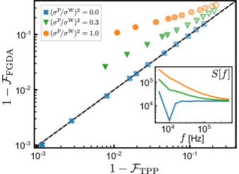
Figure 10: Comparative classification performance of FGDA versus TPP in the presence of classical correlated noise. We consider a $C=2$ (binary) dispersive qubit readout task using simulated data and for different colored noise conditions. Darker markers indicate stronger measurement tone amplitudes. The dashed line indicates $1-\mathcal{F}_{\rm FGDA}=1-\mathcal{F}_{\rm TPP}$. The inset plots the corresponding noise spectral density $S[f]$, which remains unchanged with coherent input power.

Appendix F TPP learning of correlated classical noise

In this appendix section, we use a further example to demonstrate the ability of TPP-based learning to extract correlations from measured data, to supplement simulations in Sec. V. Like Sec. V.2, we again consider simulated datasets of measured heterodyne records from a measurement chain of a qubit-cavity-amplifier setup, as in Sec. III.2. Now, however, we consider the excess classical noise added by the measurement process to also possess a component with a colored spectrum (suppressing quadrature labels for clarity):

$$\xi^{\rm cl}(t_{i})=\sigma^{\rm W}\xi^{\rm W}(t_{i})+\sigma^{\rm P}\xi^{\rm P}(t_{i})$$ (112)

where $\xi^{\rm W}(t_{i})$ describes white noise as before, while $\xi^{\rm P}(t_{i})$ describes $1/f$ (or pink) noise. The power spectral density of the noise processes is given by the Fourier transform of their steady-state autocorrelation function (by the Wiener-Khinchin theorem), $S_{\rm N}[f]=\int d\tau\leavevmode\nobreak\ e^{-i2\pi f\tau}\mathbb{E}[\xi^{\rm N}(0)\xi^{\rm N}(\tau)]$ for ${\rm N}\in\{\rm W,P\}$. The noise processes are normalized so that the total noise power, $\int df\leavevmode\nobreak\ |S_{\rm N}[f]|$ is the same for any of the considered noise processes; hence the relative magnitude $(\sigma^{\rm P}\!/\sigma^{\rm W})^{2}$ determines the relative strength of the noise processes with different correlation statistics.

We restrict ourselves again to binary classification of states $\ket{e}$ and $\ket{g}$. In Fig. 10, we plot the calculated infidelities using the MF and TPP approaches against each other in logscale for different noise conditions parameterized by $(\sigma^{\rm P}\!/\sigma^{\rm W})^{2}$, and as a function of the coherent input tone power: darker markers correspond to readout with stronger input tones.

We immediately see that if the excess classical noise is purely white, the FGDA and TPP exhibit very similar performance: both lie along the dashed line of equal infidelities. However, the situation is very different if the added noise is colored, namely $(\sigma^{\rm P}\!/\sigma^{\rm W})^{2}\neq 0$, and hence has a non-zero correlation timescale. We immediately note that even when the colored noise powers is only a fraction of the white noise power, the TPP-learned filters provide a non-negligible improvement over the standard MF scheme.