Learning to design protein–protein interactions with enhanced generalization

Abstract

Discovering mutations enhancing protein–protein interactions (PPIs) is critical for advancing biomedical research and developing improved therapeutics. While machine learning approaches have substantially advanced the field, they often struggle to generalize beyond training data in practical scenarios. The contributions of this work are three-fold. First, we construct PPIRef, the largest and non-redundant dataset of 3D protein–protein interactions, enabling effective large-scale learning. Second, we leverage the PPIRef dataset to pre-train PPIformer, a new SE(3)-equivariant model generalizing across diverse protein-binder variants. We fine-tune PPIformer to predict effects of mutations on protein–protein interactions via a thermodynamically motivated adjustment of the pre-training loss function. Finally, we demonstrate the enhanced generalization of our new PPIformer approach by outperforming other state-of-the-art methods on new, non-leaking splits of standard labeled PPI mutational data and independent case studies optimizing a human antibody against SARS-CoV-2 and increasing the thrombolytic activity of staphylokinase.

1 Introduction

The goal of this work is to develop a reliable method for designing protein–protein interactions (PPIs). We focus on predicting binding affinity changes of protein complexes upon mutations. This problem, also referred to as $\Delta\Delta G$ prediction, is the central challenge of protein binder design (Marchand et al., 2022). The discovery of mutations increasing binding affinity unlocks application areas of tremendous importance, most notably in healthcare and biotechnology. Interactions between proteins play a crucial role in mechanisms of various diseases including cancer and neurodegenerative diseases (Lu et al., 2020; Ivanov et al., 2013). Simultaneously, they offer potential pathways for the action of protein-based therapeutics in addressing other medical conditions, such as stroke, which stands as a leading cause of disability and mortality worldwide (Feigin et al., 2022; Nikitin et al., 2022). Furthermore, the design of PPIs is also relevant to biotechnological applications, including the development of bio-sensors (Scheller et al., 2018; Langan et al., 2019).

While machine learning methods for designing protein–protein interactions have been developed for more than a decade, their generalization beyond training data is hindered by multiple challenges. First, training datasets for protein–protein interactions suffer from severe redundancy and biases. These inherent imperfections are difficult to identify and rectify using available algorithmic tools due to their low scalability. Second, the approaches employed for train-test splitting of both large-scale unlabeled PPIs and small mutational libraries introduce data leakage, where interactions with near-duplicate 3D structures appear both in the training and test sets. As a result, performance estimates of machine learning models do not accurately reflect their real-world generalization capabilities. Besides that, commonly employed evaluation metrics do not fully capture practically important performance criteria. Finally, the design and training of the existing models for predicting binding affinity changes upon mutations are often prone to overfitting, as they do not fully capture the right granularity of the protein complex representation and the appropriate inductive biases.

In this work, we make a step towards more generalizable machine learning for the design of protein–protein interactions. The contribution of our work is threefold. First, we exhaustively mine the Protein Data Bank to establish a novel, complete and non-redundant dataset of 3D structures of protein–protein interactions, which we name PPIRef. Our dataset exceeds the other alternatives of its kind in terms of both size and quality. To achieve the higher quality, we develop iDist, a scalable algorithm for comparing the 3D structures of protein–protein interfaces, and apply it to cluster and debias our dataset. Furthermore, we apply iDist to evaluate the redundancy of other datasets and to illustrate the data leakage issue inherent in existing data splits. Second, we develop PPIformer – an $SE(3)$-equivariant transformer for modeling the coarse-grain structures of PPIs. Utilizing PPIRef, we pre-train PPIformer to generalize across diverse variants of protein binders. We propose and analyze the data representation and regularization techniques to maximize the generalization capabilities of our model. Finally, we fine-tune PPIformer on the task of predicting binding affinity changes of protein–protein interactions upon mutations ($\Delta\Delta G$). To achieve effective transfer learning, we utilize a modified pre-training loss function, where the modification is inspired by the thermodynamic definition of $\Delta\Delta G$. Further, we create a higher-quality data split of existing mutational data and rethink the evaluation metrics. We demonstrate that our method outperforms state-of-the-art machine learning models on multiple test sets which include case studies on designing a human antibody targeting SARS-CoV-2 and engineering the staphylokinase thrombolytic for higher activity.

In summary, our work introduces a new state-of-the-art machine learning model for designing protein–protein interactions, as well as the largest and non-redundant dataset of protein–protein interactions along with an algorithm for finding near duplicates in large-scale PPI data. We plan to make both the model and the data publicly available.

2 Related work

Predicting the effects of mutations on protein–protein interactions.

The task of predicting the effects of mutations on protein–protein interactions measured by $\Delta\Delta G$ has been studied for more than a decade (Geng et al., 2019b). Traditionally, $\Delta\Delta G$ predictors relied on physics-based simulations and statistical potentials (Barlow et al., 2018; Xiong et al., 2017; Dehouck et al., 2013; Schymkowitz et al., 2005). In contrast, more recent machine learning approaches (Rodrigues et al., 2021; Pahari et al., 2020; Wang et al., 2020; Geng et al., 2019a) primarily rely on handcrafted descriptors of protein–protein interfaces. The latest generation of the methods employs end-to-end deep learning from protein complexes, claiming to surpass computationally intensive force field simulations in terms of predictive performance (Luo et al., 2023; Shan et al., 2022; Liu et al., 2021). In this study, we revisit this claim and show that the reported performance of the state-of-the-art methods may be overestimated due to leaks in the evaluation data and overfitting.

Self-supervised learning for protein design.

Collecting annotated mutational data is resource-intensive, prompting exploration into self-supervised learning to reduce dependency on small labeled datasets. Notably, protein language models have demonstrated competitive performance without any supervision by utilizing raw inferred amino acid type probabilities (Meier et al., 2021). Similarly, protein inverse folding methods were shown to effectively predict the effects of single-point mutations on protein complex stability (Hsu et al., 2022). Likewise, predicting missing amino acids in full-atomic protein structures was shown to be effective for detecting mutation hotspots (Shroff et al., 2019). Recently, Zhang et al. (2023) have demonstrated enhanced predictive performance on multiple downstream problems achieved through self-supervised pre-training on synthetic proxy tasks on protein structures. Some of the latest binding $\Delta\Delta G$ predictors utilize pre-training from monomeric protein structures by learning to reconstruct native side chain rotamer angles (Luo et al., 2023; Liu et al., 2021). In this study, we introduce a self-supervised model pre-trained on 3D structures of protein–protein interactions for the downstream engineering of protein binders.

Datasets of protein–protein interactions.

[] Dataset PPI Unique structures interfaces MaSIF-search 6K 5K DIPS / DIPS-Plus 40K 9K PPIRef (ours) 322K 46K (PPIRef50K)

Figure 1: Comparison of PPIRef with existing datasets of native protein complexes.

Figure 2: Comparison of our PPIRef dataset with existing datasets of native protein complexes. The number of unique interfaces is estimated by deduplication using our iDist algorithm.

Historically, datasets of protein–protein interactions have been falling under two categories: sets of hundreds of small curated task-specific examples (Jankauskaitė et al., 2019; Vreven et al., 2015), and larger collections of thousands of unannotated interactions, potentially containing biases and structural redundancy (Morehead et al., 2021; Evans et al., 2021; Townshend et al., 2019; Gainza et al., 2020). In this work, we construct a new dataset that is one order of magnitude larger than existing alternatives from the second category. We further refine our dataset by removing structurally near-duplicate entries using our new scalable 3D structure-matching algorithm. This results in the largest available and non-redundant dataset of protein–protein interaction structures. Our algorithm for comparing protein–protein interactions contrasts with existing methods that rely on computationally intensive alignment procedures (Shin et al., 2023b; Mirabello & Wallner, 2018; Cheng et al., 2015; Gao & Skolnick, 2010a). Instead, we design our algorithm to enable large-scale retrieval of similar protein–protein interfaces by approximating their structural alignment. Our approach stands in line with prior work on the efficient retrieval of similar protein sequences (Steinegger & Söding, 2017), and more recently, monomeric protein structures (van Kempen et al., 2023).

3 PPIRef: New large dataset of protein–protein interactions

The Protein Data Bank (PDB) is a massive resource of over 200,000 experimentally obtained protein 3D structures (Berman et al., 2000). The space of protein–protein interactions in PDB is hypothesized to cover nearly all physically plausible interfaces in terms of geometric similarity (Gao & Skolnick, 2010b). Nevertheless, it comes at the expense of a heavy structural redundancy given by the highly modular anatomy of many proteins and their complexes (Draizen et al., 2022; Burra et al., 2009). To the best of our knowledge, there have been no attempts to quantitatively assess the redundancy of the large protein–protein interaction space represented in PDB and construct a balanced subset suitable for large-scale learning. We start this section by introducing the approximate iDist algorithm enabling fast detection of near duplicate protein–protein interfaces (Section 3.1). Using iDist, we assess the effective size and splits of existing PPI datasets (Section 3.2) and propose a new, largest and non-redundant PPI dataset, called PPIRef (Section 3.3).

3.1 iDist: new efficient approach for protein–protein interface deduplication

[]

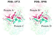
Figure 3: An example of protein–protein interfaces from the different folds of the DIPS dataset detected as near duplicates by our iDist method. Both PPIs come from the same KatE enzyme homooligomers with different single-point mutations. Notably, the symmetry of the complex itself yields 3 groups of 2 duplicates (from a single PDB entry with 6 PPIs). Furthermore, querying PDB with “KatE” results in 36 KatE complexes, yielding, therefore, 3 groups of 72 duplicates each. Our iDist approach can efficiently identify such structural near duplicates on a large scale.

Existing algorithms to determine the similarity between protein–protein interfaces rely on structural alignment procedures (Gao & Skolnick, 2010a; Mirabello & Wallner, 2018; Shin et al., 2023a). However, since finding an optimal alignment between PPIs is computationally heavy, alignment-based approaches do not scale to large datasets. Therefore, we develop a reliable approximation of the well established algorithm iAlign, which adapts the well-known TM-score to the domain of PPIs (Gao & Skolnick, 2010a). Our iDist algorithm calculates $SE(3)$-invariant vector representations of protein–protein interfaces via message passing between residues, which in turn enables efficient detection of near-duplicates using the Euclidean distance with a threshold estimated to approximate iAlign (Figure 6). The complete algorithm is described in Appendix A.

To evaluate the performance of our iDist, we benchmark it against iAlign. We start by sampling 100 PDB codes from the DIPS dataset (Townshend et al., 2019) of protein–protein interactions and extract the corresponding 1,646 PPIs. Subsequently, we calculate all 2,709,316 pairwise similarities between these PPIs using both the exact iAlign structural alignment algorithm and our efficient iDist approximation. Employing 128 CPUs in parallel, iAlign computations took 2 hours, while iDist required 15 seconds, being around 480 times faster. Next, we estimate the quality of the approximation on the task of retrieving near-duplicate PPI interfaces. Using iAlign-defined ground-truth duplicates, iDist demonstrates a precision of 99% and a recall of 97%. These evaluation results confirm that iDist enables efficient structural deduplication of extensive PPI data within a reasonable timeframe, which is not achievable with other existing algorithms. The scalability of the method enabled us to analyze existing PPI datasets and their respective data splits used by the recent machine-learning approaches. The analysis is described below. Please refer to Appendix A for the additional details of the evaluation of iDist.

3.2 Limitations of existing protein–protein interaction datasets

We apply iDist to assess the composition of DIPS – the state-of-the-art dataset of protein–protein interactions comprising approximately 40,000 entries (Morehead et al., 2021; Townshend et al., 2019). We construct a near-duplicate graph of DIPS by connecting two protein–protein interfaces if they are detected as near duplicates by iDist (see Figure 3 for an example). This results in a graph with 8.5K connected components, where the largest connected component comprises 36% of the interfaces. Notably, relaxing iDist duplicate detection threshold 1.5 times results in 84% of the interfaces forming a single component, indicating the high connectivity of the PPI space in DIPS. After iteratively deduplicating entries with at least one near duplicate, the dataset size drops to 22% of its initial size. These observations are in agreement with the hypothesis of Gao & Skolnick (2010b) suggesting high connectivity and redundancy of the PPI space in PDB. Finally, we analyze the existing data splits of DIPS. We estimate the leakage ratio of a split by finding the percentage of test interactions having near duplicates in the training or the validation fold. We find that the split based on protein sequence similarity (not 3D structure as in our case) used for the validation of protein–protein docking models (Ketata et al., 2023; Ganea et al., 2021) has near duplicates in the training data for 53% of test examples, while the random split from (Morehead et al., 2021) has 88% of test examples with a near duplicate in the training data. Figure 3 illustrates an example of such a leak: the interface on the left-hand side is present in the test fold of the original split (Ganea et al., 2021), while the interface on the right-hand side is in the training fold.

3.3 PPIRef: New large dataset of protein–protein interactions

We address the redundancy of existing PPI datasets by building a novel dataset of structurally distinct 3D protein–protein interfaces. We call the new dataset PPIRef. We start by exhaustively mining all 202,380 entries from the Protein Data Bank as of June 20, 2023. Subsequently, we extract all putative interactions by finding all pairs of protein chains that have a contact between heavy atoms in the range of at most $10\mathrm{\mathring{A}}$. This procedure results in 837,241 hypothetical PPIs, further referred to as the raw PPIRef800K. Further, we apply the well-established criteria (Appendix A, Townshend et al. (2019)) to select only biophysically proper interactions. This filtering results in 322,454 protein–protein interactions comprising the vanilla version of PPIRef, which we name PPIRef300K. Finally, we iteratively filter out near-duplicate entries by applying the iDist algorithm. This deduplication results in the final non-redundant dataset comprising 45,553 PPIs, which we call PPIRef50K (or simply PPIRef). Figure 2 illustrates that our dataset exceeds the sizes and effective sizes of the representative alternatives DIPS (Townshend et al., 2019), DIPS-Plus (Morehead et al., 2021) and the one used to train the MaSIF-search model (Gainza et al., 2020), also used by the recent MaSIF-seed pipeline for de novo PPI design (Gainza et al., 2023).

4 Learning to design protein–protein interactions

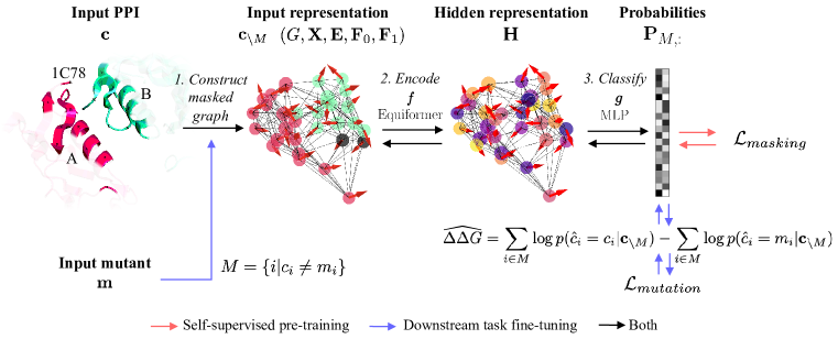
Figure 4: Overview of PPIformer. A single pre-training step starts with randomly sampling a protein–protein interaction $\mathbf{c}$ (in this example, the staphylokinase dimer A-B from the PDB entry 1C78). Next, randomly selected residues $M$ are masked to obtain the masked interaction $\mathbf{c}_{\setminus M}$. After that, the interaction is converted into a graph representation $(G,\mathbf{X},\mathbf{E},\mathbf{F}_{0},\mathbf{F}_{1})$ with masked nodes $M$ (black circles). The model subsequently learns to classify the types of masked amino acids by acquiring $SE(3)$-invariant hidden representation $\mathbf{H}$ of the whole interface via the encoder $f$ and classifier $g$. On the downstream task of $\Delta\Delta G$ prediction (blue arrows), mutated amino acids are masked, and the probabilities of possible substitutions $\mathbf{P}_{M,:}$ are jointly inferred with the pre-trained model. Finally, the estimate $\widehat{\Delta\Delta G}$ is obtained using the predicted probabilities $p$ of the wild-type $c_{i}$ and the mutant $m_{i}$ amino acids via log odds.

Predicting differences in binding energies ($\Delta\Delta G$) of protein complexes upon amino-acid substitutions is a core problem in the design of protein–protein interactions. However, the task of $\Delta\Delta G$ prediction is challenging for machine learning due to the scarcity of available annotated datasets, which cover only several hundred protein–protein interactions (Jankauskaitė et al., 2019). In this section, we first discuss our coarse-grain representations of proteins that enable modeling protein complexes and their mutants in a way robust to overfitting (Section 4.1). Second, we introduce the PPIformer model architecture, which efficiently operates on the representations through its $SE(3)$-equivariance (Section 4.2). Third, we describe our masking procedure and a loss function that enables us to pre-train PPIformer on 3D PPIs from the PPIRef dataset (Section 4.3). Finally, we demonstrate how the pre-trained PPIformer can be seamlessly fine-tuned to predict $\Delta\Delta G$ values by leveraging masked modeling and a thermodynamically inspired loss function (Section 4.4).

4.1 Representation of protein–protein complexes

In a living cell, proteins continually undergo thermal fluctuations and change their precise shapes. This fact is particularly manifested on protein surfaces, where the precise atomic structure is flexible due to interactions with other molecules. As a result, protein–protein interfaces may be highly flexible (Kastritis & Bonvin, 2013). Nevertheless, the available crystal structures from the Protein Data Bank only represent their rigid, energetically favorable states (Jin et al., 2023). Therefore, we aim to develop representations of protein complexes robust to atom fluctuations, as well as well-suited for modeling mutated interface variants. In this section, we define a coarse residue-level representation to allow for sufficient flexibility of the interfaces, which nevertheless captures the major aspects of the interaction patterns.

More specifically, consider a protein–protein complex (or interface) $\mathbf{c}\in\mathbb{\mathcal{A}}^{N}$ of $N$ residues in the alphabet of amino acids $\mathcal{A}=\{1,\dots,20\}$. We consider the order of residues in $\mathbf{c}$ arbitrary, ensuring permutation invariance, a property critical for representing the interfaces (Mirabello & Wallner, 2018). Next, we represent the complex $\mathbf{c}$ as a $k$-NN graph $G$, where the nodes represent the individual residues and edges are based on the proximity of corresponding alpha-carbon ($C_{\alpha}$) atoms. The graph is augmented by node-level and pair-wise features $\mathbf{X},\mathbf{E},\mathbf{F}_{0},\mathbf{F}_{1}$. In detail, matrix $\mathbf{X}\in\mathbb{R}^{N\times 3}$ contains the coordinates of alpha-carbons of all residues. Next, all residue nodes are put into semantic relation by pair-wise binary edge features $\mathbf{E}\in\{0,1\}^{N\times N}$ with 0 if residues come from the same protein partner and 1 otherwise. Finally, each node is associated with two kinds of features: type-0 $\mathbf{F}_{0}\in\mathbb{R}^{N\times 20\times 1}$, also referred to as scalars, and type-1 vectors $\mathbf{F}_{1}\in\mathbb{R}^{N\times 1\times 3}$. Features $\mathbf{F}_{0}$ capture the one-hot representations of wild-type amino acids $\mathbf{c}$, while vectors $\mathbf{F}_{1}$ are defined as virtual beta-carbon orientations calculated from the backbone geometry using ideal angle and bond length definitions (Dauparas et al., 2022). Please note that $\mathbf{F}_{0}$ are invariant with respect to rototranslations and $\mathbf{F_{1}}$ are equivariant. Collectively, coordinates $\mathbf{X}$ and virtual-beta carbon directions $\mathbf{F_{1}}$ capture the complete geometry of the protein backbones involved in the complex. Our representation is agnostic to precise angles of side-chain rotamers, implicitly modeling their flexibility. The schematic illustration is provided in Figure 4 (Input representation).

4.2 PPIformer model

In order to effectively learn from protein–protein complexes or interfaces $(G,\mathbf{X},\mathbf{E},\mathbf{F}_{0},\mathbf{F}_{1})$, i.e. respecting permutation invariance of amino acids and arbitrary coordinate systems of Protein Data Bank entries, we define PPIformer, an $SE(3)$-equivariant architecture. The model consists of an encoder $f$ and classifier $g$ such that $g(f(G,\mathbf{X},\mathbf{E},\mathbf{F}_{0},\mathbf{F}_{1}))$ yields a probability matrix $\mathbf{P}\in[0,1]^{N\times|\mathcal{A}|}$, where $P_{i,j}$ defines the probability of amino-acid type $j$ at residue $i$. Intuitively, matrix $\mathbf{P}$ captures the likelihood of amino acids to occur at different positions in a protein complex depending on their structural context.

The core of our architecture is comprised of Equiformer $SE(3)$-equivariant graph attention blocks $f^{(l)}$ (Liao et al., 2023; Liao & Smidt, 2022). Each of the $L$ blocks (or layers) updates equivariant features of different types associated with all amino acids via message passing with an equivariant attention mechanism with $K$ heads. In detail, the input to the $l$^th block is an original graph $G$ with coordinates $\mathbf{X}$ and edge features $\mathbf{E}$ along with a set of node feature matrices $\mathbf{H}_{k}^{(l)}\in\mathbb{R}^{N\times d_{k}\times(2k+1)}$ of different equivariance types $k\geq 0$ from the previous layer. Here, $d_{k}\geq 0$ is a hyper-parameter defining the number of type-$k$ hidden features shared across all blocks, and $2k+1$ is their corresponding theoretical dimension. The input node features for the first layer are set to $\mathbf{F}_{0},\mathbf{F}_{1}$. The output of each block is given by the updated node features of different equivariance types. Internally, all blocks lift hidden features up to the equivariant representations of the degree $\deg\geq 0$ which is an additional hyper-parameter. Taking the type-0 outputs of the final layer leads to invariant amino acid embeddings $\mathbf{H}$ as:

$$\mathbf{H}^{(1)}_{0},\mathbf{H}^{(1)}_{1},\dots,\mathbf{H}^{(1)}_{deg} =f^{(0)}(G,\mathbf{X},\mathbf{E},\mathbf{F}_{0},\mathbf{F}_{1}),$$ (1)

$$\mathbf{H}^{(l+1)}_{0},\mathbf{H}^{(l+1)}_{1},\dots,\mathbf{H}^{(l+1)}_{deg} =f^{(l)}(G,\mathbf{X},\mathbf{E},\mathbf{H}^{(l)}_{0},\mathbf{H}^{(l)}_{1},\dots,\mathbf{H}^{(l)}_{deg}),$$ (2)

$$\mathbf{H} :=\mathbf{H}^{(L-1)}_{0}.$$ (3)

Collectively, we term the composition of transformer blocks $f^{(l)}$ (for $l\in\{0,\dots,L-1\}$) as the encoder

$$f :G,\mathbf{X},\mathbf{E},\mathbf{F}_{0},\mathbf{F}_{1}\mapsto\mathbf{H}$$ (4)

with the property of $SE(3)$-invariance for any rotation $\mathbf{R}\in SO(3)$ and translation $\mathbf{t}\in\mathbb{R}^{3}$:

$$f(G,\mathbf{X},\mathbf{E},\mathbf{F}_{0},\mathbf{F}_{1}) =f(G,\mathbf{X}\mathbf{R}+\mathbf{1}\mathbf{t}^{T},\mathbf{E},\mathbf{F}_{0},\mathbf{F}_{1}).$$ (5)

To further estimate the probabilities of masked amino acids discussed below, we apply a 1-layer classifier with the softmax activation $g:\mathbb{R}^{N\times d_{0}\times 1}\to[0,1]^{N\times\mathcal{|A|}}$ on top of node embeddings $\mathbf{H}$ to obtain the probability matrix $\mathbf{P}$.

4.3 3D equivariant self-supervised pre-training from unlabeled protein–protein interactions

In this section, we describe how we leverage a large amount of unlabeled protein–protein interfaces from PPIRef to train our model for predicting the effects of mutations on binding affinity. We first present the pre-training method used to effectively train PPIformer to capture the space of native variants of binding interfaces. Then, we discuss the fine-tuning of our model to predict the effects of mutations via log odds ratios. Finally, we demonstrate that the proposed combination of masked pre-training and log-odds fine-tuning is well-justified thermodynamically.

Structural masking of protein–protein interfaces.

The paradigm of masked modeling has proven to be an effective way of pre-training from protein sequences (Lin et al., 2023). Nevertheless, while the masking of amino acids in a protein sequence is straightforward by introducing a special token, the masking of structural fragments is not obvious. Here, we leverage our flexible coarse-grain protein–protein complex representation to define masking by a simple change in the feature representation.

Having a protein complex or interface $\mathbf{c}\in\mathcal{A}^{N}$ containing $N$ amino acids from vocabulary $\mathcal{A}$ and a mask $M\subset\{1,\dots,N\}$, we define the masked structure $\mathbf{c}_{\setminus M}\in(\mathbb{\mathcal{A}}\cup\{0\})^{N}$ by setting amino acid classes at all masked positions $M$ to zeros. Consequently, when constructing one-hot scalar features $\mathbf{F}_{0}$ from $\mathbf{c}_{\setminus M}$, we set the corresponding rows to zeroes. Note that vector features $\mathbf{F}_{1}$ do not require masking since they do not contain any information about the types of amino acids, benefiting from using virtual beta-carbons instead of real ones. Additionally, the glycine amino acid, which lacks the beta-carbon atom, does not need special handling.

Loss for masked modeling of protein–protein interfaces.

Having a protein–protein interaction and a random mask $M\subset\{1,\dots,N\}$, we follow a traditional cross-entropy loss for training the model to predict native amino acids in a masked version $\mathbf{c}_{\setminus M}\in(\mathbb{\mathcal{A}}\cup\{0\})^{N}$ of the native complex $\mathbf{c}\in\mathbb{\mathcal{A}}^{N}$. To additionally increase the generalization capabilities of PPIformer to capture potentially unseen or mutated interfaces, we further employ two regularization measures. First, we apply label smoothing to force the model not to be overly confident in native amino acids, so that it can be more flexible towards unseen variants (Szegedy et al., 2016). Second, we weight the loss inversely to the prior distribution of amino acids in protein–protein interfaces to remove the bias towards overrepresented amino acids such as leucine. The overall pre-training loss is defined as

$$\mathcal{L}_{masking} =-\sum_{i\in M}{w_{c_{i}}\Biggl{[}(1-\epsilon)\cdot\log{p(\hat{c}_{i}=c_{i}|\mathbf{c}_{\setminus M})}+\epsilon\sum_{j\in\mathcal{A}\setminus c_{i}}{\log{p(\hat{c}_{i}=c_{j}|\mathbf{c}_{\setminus M})}\cdot\frac{1}{|\mathcal{A}|}\Biggr{]}}}.$$ (6)

Here, $p(\hat{c}_{i}=c_{i}|\mathbf{c}_{\setminus M}):=P_{i,c_{i}}$ is the probability of predicting the native amino acid type $c_{i}$ of a masked residue $i\in M$. Next, the sum over all other, non-native, amino acid types $j\in\mathcal{A}\setminus c_{i}$ is the label smoothing regularization term where $0<\epsilon<1$ is the smoothing hyper-parameter. Further, $w_{c_{i}}$ is the weighting factor corresponding to the native amino acid $c_{i}$. Finally, the sum over $i\in M$ corresponds to the loss being evaluated over all masked residues.

4.4 Transfer learning for predicting the effects of mutations on protein–protein interactions

Predicting the effects of mutations on binding affinity ($\Delta\Delta G$) is a central task in designing protein–protein interactions. Nevertheless, collecting $\Delta\Delta G$ annotations is expensive and time-consuming. As a result, the labeled mutational data for binding affinity changes are scarce, not exceeding several thousand annotations (Jankauskaitė et al., 2019). Therefore, in our work, we aim to leverage the pre-trained PPIformer model for scoring mutations with minimal supervision.

Thermodynamic motivation.

From the thermodynamic perspective, binding energy change $\Delta\Delta G$ (or alternatively denoted as $\Delta\Delta G_{wt\rightarrow mut}$) can be decomposed as follows:

$$\Delta\Delta G =\Delta G_{mut}-\Delta G_{wt}=RT(\log{(K_{wt})}-\log{(K_{mut})}),$$ (7)

where $\Delta G_{mut}$ and $\Delta G_{wt}$ are binding energies of mutated and wild-type complexes, respectively (Kastritis & Bonvin, 2013). The $R,T>0$ terms are gas and temperature environmental constants, and $K_{wt}$ and $K_{mut}$ denote the equilibrium constants of protein–protein interactions, i.e. the ratios of the concentration of the complexes formed when proteins interact to the concentrations of the individual proteins. The form of $\Delta\Delta G$ (Equation 7) introduces symmetries into the problem of estimating the quantity. For example, predicting the effect of a reversed mutation $\Delta\Delta G_{mut\rightarrow wt}$ should satisfy the antisymmetry property $\Delta\Delta G_{wt\rightarrow mut}=-\Delta\Delta G_{mut\rightarrow wt}$. Available machine learning predictors either ignore the symmetry (Liu et al., 2021) or require two forward passes to estimate the quantity twice, for both directions, and combine the predictions to enforce the antisymmetry as ($\Delta\Delta G_{wt\rightarrow mut}-(-\Delta\Delta G_{mut\rightarrow wt}))/2$ (Luo et al., 2023).

Predicting the effects of mutations on binding energy via the log odds ratio.

Here, in line with physics-informed machine learning (Karniadakis et al., 2021), we leverage the thermodynamic interpretation of $\Delta\Delta G$ to adapt the pre-training cross-entropy for the downstream $\Delta\Delta G$ fine-tuning. Having a complex $\mathbf{c}\in\mathbb{\mathcal{A}}^{N}$ and its mutant $\mathbf{m}\in\mathbb{\mathcal{A}}^{N}$, with the substitutions of residues $M\subset\{1,\dots,N\}$ such that $c_{i}\neq m_{i}$ for all $i\in M$, we estimate its binding energy change as:

$$\widehat{\Delta\Delta G} =\sum_{i\in M}{\log{p(\hat{c}_{i}=c_{i}|\mathbf{c}_{\setminus M})}}-\sum_{i\in M}{\log{p(\hat{c}_{i}=m_{i}|\mathbf{c}_{\setminus M})}},$$ (8)

where the $p$ terms are PPIformer output probabilities. The $\widehat{\Delta\Delta G}$ prediction is the log odds ratio, used by Meier et al. (2021) for zero-shot predictions on protein sequences. Intuitively, the predicted binding energy change upon mutation is negative (increased affinity) if the predicted likelihood of the mutated structure is higher than the likelihood of the native structure. When simultaneously decomposing Equation 7 and Equation 8, we observe that $\log{(K_{wt})}$ is estimated as $\sum_{i\in M}{\log{p(\hat{c}_{i}=c_{i}|\mathbf{c}_{\setminus M})}}$, and $\log{(K_{mut})}$ is estimated as $\sum_{i\in M}{\log{p(\hat{c}_{i}=m_{i}|\mathbf{c}_{\setminus M})}}$. Considering that the estimate of the wild-type likelihood is identical to the pre-training loss (Equation 6) up to the regularizations, we reason that during pre-training PPIformer learns the correlates of $\Delta G$ values, whereas during fine-tuning it refines them to $\Delta\Delta G$ predictions. For the fine-tuning through Equation 8, we use the MSE loss denoted as $\mathcal{L}_{mutation}$.

5 Experiments

In this section, we describe our protocol for benchmarking the generalization on the task of $\Delta\Delta G$ prediction and present our results. We begin by introducing the evaluation datasets, metrics, and baseline methods (Section 5.1). Next, we show that our approach outperforms state-of-the-art machine learning methods in designing protein–protein interactions distinct from the training data (Section 5.2). Additionally, we show the benefits of our new PPIRef dataset and key PPIformer components through several ablation studies in Appendix C.

5.1 Evaluation protocol

Datasets.

To fine-tune PPIformer for $\Delta\Delta G$ prediction we use the largest available labeled dataset, SKEMPI v2.0, containing 7085 mutations (Jankauskaitė et al., 2019). Prior works (Luo et al., 2023; Liu et al., 2021) primarily validate the performance of models on PDB-disjoint splits of the dataset. However, we find such approach not appropriate to measure the generalization capacity of predictors due to a high ratio of leakages. Therefore, we construct a new, non-leaking cross-validation split and set aside 5 PPI outliers to obtain 5 distinct test folds. Further, to simulate practical protein–protein interaction design scenarios, we perform additional evaluation on two independent case studies. These case studies assess the capability of models to retrieve mutations optimizing the human P36-5D2 antibody against SARS-CoV-2 and increasing the thrombolytic activity of staphylokinase. Please refer to Section B.2 for details.

Metrics.

To evaluate the capabilities of models in prioritizing favorable mutations, we use the Spearman correlation coefficient between the predicted and ground-truth $\Delta\Delta G$ values. To evaluate the performance in detecting stabilizing mutations, we calculate precision and recall with respect to negative $\Delta\Delta G$ values. We also report additional metrics to enable comparison with prior work (Luo et al., 2023). However, in Section B.3, we emphasize that these metrics can be misleading when selecting a model for a practical application. For the independent retrieval case studies, we report the predicted ranks for all favorable mutations and evaluate the retrieval performance using the precision at $k$ metrics (P@$k$). We provide the details in Section B.3.

Baselines.

We evaluate the performance of PPIformer against the state-of-the-art represenatives of four main categories of available methods. Specifically, the Flex ddG (Barlow et al., 2018) Rosetta-based (Leman et al., 2020) protocol is the most advanced traditional force-field simulator (the same protocol is used in a recent RosettaDDGPrediction toolbox (Sora et al., 2023)). The baseline machine learning methods are: supervised RDE-Network (Luo et al., 2023), pre-trained on unlabeled monomer protein structures and fine-tuned for $\Delta\Delta G$ prediction on SKEMPI v2.0; ESM-IF (Hsu et al., 2022), an unsupervised predictor of $\Delta\Delta G$ trained for inverse folding on experimental and AlphaFold2 (Jumper et al., 2021) structures; and MSA Transformer (Rao et al., 2021), an evolutionary baseline. A more detailed description of the methods and their settings is provided in Section B.4.

5.2 Comparison with the state of the art

Prediction of $\Delta\Delta G$ on held-out test cases.

As shown in Table 1, on 5 challenging test PPIs from SKEMPI v2.0, PPIformer confidently outperforms all machine-learning baselines in 6 out of 7 evaluation metrics, being the second-best in terms of recall. We achieve a 173% relative improvement in mutation ranking compared to the state-of-the-art supervised RDE-Network, as measured by Spearman correlation. Importantly, this non-leaking evaluation reveals that traditional force field simulators, represented by state-of-the-art Flex ddG, still outperform machine learning methods in terms of predictive performance. However, in terms of speed, they may not be applicable in typical real-world large-scale mutational screenings, being 5 orders of magnitude slower (see Section B.4 for details).

[] Category Method Spearman $\uparrow$ Pearson $\uparrow$ Precision $\uparrow$ Recall $\uparrow$ ROC AUC $\uparrow$ MAE $\downarrow$ RMSE $\downarrow$ Force field simulations Flex ddG $0.54$ $0.57$ $0.63$ $0.62$ $0.84$ $1.60$ $2.00$ Machine learning MSA Transformer $\underline{0.37}$ $\underline{0.45}$ $0.51$ $0.38$ $\underline{0.76}$ $5.99$ $6.77$ ESM-IF $0.32$ $0.31$ $0.36$ $0.28$ $0.69$ $1.84$ $2.11$ RDE-Net. $0.24$ $0.30$ $\underline{0.54}$ 0.65 $0.67$ $\underline{1.70}$ $\underline{2.02}$ PPIformer (ours) 0.42 0.46 0.58 0.61 0.77 1.64 1.94

Table 1: Test set performance averaged across five held-out protein–protein interactions selected from SKEMPI v2.0 for benchmarking (see Section B.2 for details). The standard deviation for PPIformer is estimated from three training experiments with different random seeds.

Optimization of a human antibody against SARS-CoV-2.

Within a pool of 494 candidate single-point mutations of a human antibody, our model detects 2 mutations out of 5 (using a 10% threshold as defined by Luo et al. (2023)) that are known to be effective against SARS-CoV-2 (Table 2). The best among the other methods detects 3 out of 5 mutations. However, PPIformer achieves superior performance when considering the ranks of all 5 mutations collectively, with the maximum rank for a favorable mutation not exceeding 21.46%. Notably, in contrast to the other methods, PPIformer successfully assigns the best rank to one of the 5 favorable mutations (P@1 = 100%). Please note that given the absence of ground-truth labels for all candidate mutations, and the fact that the labeled mutations were pre-selected by DDGPred (Shan et al., 2022), it is important to emphasize that solely relying on the absolute rankings of the five annotated mutations may not accurately represent the true performance on all mutations, as the other 489 out of 494 mutants have unknown effects and may contain other favorable candidates.

[] Method TH31W $\downarrow$ AH53F $\downarrow$ NH57L $\downarrow$ RH103M $\downarrow$ LH104F $\downarrow$ P@1 $\uparrow$ P@5% $\uparrow$ P@10% $\uparrow$ MSA Transformer 56.88 42.11 63.56 49.19 18.83 0.00 0.00 0.00 Rosetta 10.73 76.72 93.93 13.56 6.88 0.00 0.00 2.04 FoldX 5.67 68.22 2.63 12.35 29.96 0.00 4.00 4.08 DDGPred 2.02 14.17 24.49 4.05 6.48 0.00 8.00 6.12 End-to-End 11.34 16.60 8.30 52.43 80.36 0.00 0.00 2.04 MIF-Net. 27.94 66.19 8.50 17.21 36.23 0.00 0.00 2.04 ESM-IF 49.39 17.61 17.00 51.42 48.58 0.00 0.00 0.00 RDE-Net. 1.62 2.02 20.65 61.54 5.47 0.00 8.00 6.12 PPIformer (ours) 18.02 0.20 7.69 21.46 10.93 100 4.00 4.08

Table 2: The performance of PPIformer and eight competing methods in retrieving 5 human antibody mutations effective against SARS-CoV-2. The middle section shows ranks (in percent) for individual mutations with predictions scored in the top 10% in bold. The right section presents precision metrics. The values for baseline methods except for MSA Transformer are reproduced from (Luo et al., 2023).

Engineering staphylokinase for enhanced thrombolytic activity.

Within a pool of 80 annotated mutations, PPIformer precisely prioritizes 2 out of 6 strongly favorable ones that increase the thrombolytic activity at least twice as the top-2 mutation candidates (Table 3). In contrast, the second-best method, RDE-Network, identifies one mutation and assigns it a worse ranking (top-4). MSA Transformer provides accurate top-1 prediction but strongly loses performance on higher cutoffs and detecting two-fold activity-increasing mutations.

[] Method Mutations with $\geq 2\times$ activity enhancement Activity enhancement KC74Q $\downarrow$ KC74R $\downarrow$ KC135R $\downarrow$ KC130E $\downarrow$ KC130T $\downarrow$ KC130A $\downarrow$ KC130T $\downarrow$ KC130T $\downarrow$ KC135A $\downarrow$ KC135R $\downarrow$ KC135R $\downarrow$ P@1 $\uparrow$ P@5% $\uparrow$ P@10% $\uparrow$ MSA Transformer 52.50 32.50 55.00 40.00 70.00 78.75 100 50.00 37.50 ESM-IF 45.00 33.75 46.25 25.00 42.50 58.75 0.00 0.00 25.00 RDE-Net. 51.25 33.75 22.50 15.00 27.50 5.00 0.00 50.00 62.50 PPIformer (ours) 66.25 15.00 2.50 52.50 33.75 1.25 100 75.00 87.50

Table 3: The performance of PPIformer and three competing methods in retrieving the mutations on the staphylokinase interface that increase its trombolytic activity via enhanced affinity to plasmin. Here, 24 of 80 mutations are favorable for activity (right section), and 6 of them lead to at least two-fold enhancement (middle section). Similarly to Table 2, the rank values in bold are those in the top-10% predictions.

6 Conclusion

In this work, we have constructed PPIRef – the largest and non-redundant dataset for self-supervised learning from protein–protein interactions. Using this data, we have pre-trained a new model, PPIformer, designed to capture diverse protein binding modes. Subsequently, we fine-tuned the model for the target task of discovering mutations enhancing protein–protein interactions. We have shown that our model effectively generalizes to unseen PPIs, outperforming other state-of-the-art machine learning methods. This work opens up the possibility of training large-scale foundation models for designing protein–protein interactions.

Acknowledgments

This work was supported by the Technology Agency of the Czech Republic through projects RETEMED (TN02000122) and TEREP (TN02000122/001N) and by the Ministry of Education, Youth and Sports of the Czech Republic through projects e-INFRA CZ [ID:90254] and ELIXIR [LM2023055]. We thank David Lacko for preparing the dataset of staphylokinase mutations.

Appendix

The first section of the appendix provides additional details on the construction of the PPIRef dataset and the evaluation of the iDist algorithm by benchmarking it against the iAlign structural alignment method (Appendix A). Next, we provide the implementation and experimental details, including the selection of training hyper-parameters, the construction of the mutation datasets, and the description of the evaluation metrics and baselines (Appendix B). Next, we discuss several ablation studies illustrating the importance of the proposed PPIformer components (Appendix C). Finally, we provide the details of the comparison of our method with the state-of-the-art $\Delta\Delta G$ predictors on the SKEMPI v2.0 test set (Appendix D).

Appendix A Details of the iDist algorithm and PPIRef dataset

In this section, we discuss the details relevant to the analysis and construction of large unannoted PPI datasets. First, we provide the complete description of the iDist deduplication algorithm and the calibration of its distance threshold. Second, we specify the construction criteria for our PPIRef.

iDist algorithm.

Algorithm 1 iDistEMBED

1:Input: Protein–protein interface $\mathcal{I}$ of $N$ residues from $C$ chains.

2:Output: Vector representation of the interface $\mathbf{z}_{\mathcal{I}}$.

3:// Get coordinates, features, and partner information

4:$\mathbf{X}\in\mathbb{R}^{N\times 3},\mathbf{F}\in\mathbb{R}^{N\times d},\mathbf{p}\in\{1,\dots,C\}^{N}\leftarrow get\_residues(\mathcal{I})$

5:// Embed residues

6:for $i\leftarrow 1$ to $N$ do

7:     $J_{intra}\leftarrow\{j\in\{1,\dots,N\}\mid p_{i}=p_{j}\}$

8:     $J_{inter}\leftarrow\{j\in\{1,\dots,M\}\mid p_{i}\neq p_{j}\}$

9:     $\mathbf{m}_{intra}\leftarrow\frac{1}{|J_{intra}|}\sum_{j\in J_{intra}}{\mathbf{f}_{j}\cdot e^{-\frac{\|\mathbf{x}_{i}-\mathbf{x}_{j}\|_{2}^{2}}{\alpha}}}$

10:     $\mathbf{m}_{inter}\leftarrow\frac{1}{|J_{inter}|}\sum_{j\in J_{inter}}{\mathbf{f}_{j}\cdot e^{-\frac{\|\mathbf{x}_{i}-\mathbf{x}_{j}\|_{2}^{2}}{\alpha}}}$

11:     $\mathbf{h}_{i}\leftarrow\frac{1}{2}\mathbf{f}_{i}+\frac{1}{4}\mathbf{m}_{intra}-\frac{1}{4}\mathbf{m}_{inter}$

12:end for

13:// Embed interface

14:for $c\leftarrow 1$ to $C$ do

15:     $J_{c}\leftarrow\{j\in\{1,\dots,N\}\mid p_{j}=c\}$

16:end for

17:$\mathbf{z}_{\mathcal{I}}\leftarrow\frac{1}{|C|}\sum_{c=1}^{C}{\frac{1}{|J_{c}|}\sum_{j\in J_{c}}{\mathbf{h}_{j}}}$

18:return $\mathbf{z}_{\mathcal{I}}$

Algorithm 2 iDist

1:Input: Two protein–protein interfaces $\mathcal{I}$ and $\mathcal{J}$.

2:Output: Distance $\geq 0$.

3:$\mathbf{z}_{\mathcal{I}}\leftarrow\text{iDistEMBED}(\mathcal{I})$

4:$\mathbf{z}_{\mathcal{J}}\leftarrow\text{iDistEMBED}(\mathcal{J})$

5:return $\|\mathbf{z}_{\mathcal{I}}-\mathbf{z}_{\mathcal{J}}\|_{2}$

Algorithms 1 and 2 outline iDist, a fast method for detecting near-duplicate protein–protein interfaces. Algorithm 1 details the conversion of a protein–protein interface $\mathcal{I}$ into a vector representation $\mathbf{z}_{\mathcal{I}}$. In the first step (line 4), the features of the interface $\mathbf{X},\mathbf{F}$ and $\mathbf{p}$ are extracted. The residue coordinates $\mathbf{X}$ are determined by the positions of the $C_{\alpha}$ atoms. Next, the residue vector features $\mathbf{F}$ are initialized with simple 20-dimensional one-hot encodings of amino acids. We have also experimented with ESM-1b features (Rives et al., 2021) but obtained slightly lower performance. We observe that the reduced performance could be attributed to ESM-1b biasing the comparison towards entire protein chains rather than the interfaces. Finally, each residue is associated with a label indicating the chain it belongs to, forming the vector $\mathbf{p}$.

[]

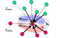
Figure 5: Illustration of the single-step message passing of iDist (lines 5-12 in Algorithm 1). A residue $i$ receives complementary distance-weighted messages $\mathbf{m}_{intra}$ and $\mathbf{m}_{inter}$ from all residues within the same protein $J_{intra}$ and other partners $J_{inter}$. The messages are aggregated into the embedding $\mathbf{h}_{i}$ and the procedure is repeated for each interface residue. iDist efficiently detects near-duplicate PPIs as the ones having similar averaged interface embeddings.

In the following steps 5-12, depicted in Figure 5, the hidden representation $\mathbf{h}_{i}$ for each residue $i$ is constructed. A residue $i$ receives messages from all other residues in both the same chain ($J_{intra}$) and the partnering chains ($J_{inter}$), represented by exponential radial basis functions with $\alpha$ set to 16. The messages are then averaged to create contact patterns $\mathbf{m}_{intra}$ and $\mathbf{m}_{inter}$. The final representation $\mathbf{h}_{i}$ is obtained by averaging the difference $\mathbf{m}_{intra}-\mathbf{m}_{inter}$, followed by averaging with the features $\mathbf{f}_{i}$. The difference heuristic is inspired by the complementarity nature of many non-covalent bonds governing PPIs. When amino acids in both the intra- and inter-contexts of a residue are similar (i.e. not small–bulky or negatively–positively charged), the message $\mathbf{m}_{intra}-\mathbf{m}_{inter}$ is low.

Lastly, in steps 13-18, the interface representation $\mathbf{z}_{\mathcal{I}}$ is derived by averaging the hidden features across the individual chains and then across the interaction. As described in Algorithm 2, iDist then simply calculates the Euclidean distance between two representations $\mathbf{z}_{\mathcal{I}}$ and $\mathbf{z}_{\mathcal{J}}$ to compare two interfaces $\mathcal{I}$ and $\mathcal{J}$. The outlined procedure can be seen as an implicit approximation of the structural alignment as the resulting representations are $SE(3)$-invariant.

iDist evaluation and threshold selection.

In order to evaluate the approximation performance of iDist we compare it with the structural alignmnet algorithm iAlign (Gao & Skolnick, 2010a), the adaptation of TM-score (Zhang & Skolnick, 2004) to protein–protein interfaces. Figure 6 shows two main modes of the joint probability distribution of the scores output by both methods. For the scores where iAlign($\mathcal{I},\mathcal{J})<0.7$ and iDist$(\mathcal{I},\mathcal{J})>0.04$, the interfaces $\mathcal{I}$ and $\mathcal{J}$ are typically distinct with rare cases of sharing similar structural patterns. In contrast, for the scores where iAlign($\mathcal{I},\mathcal{J})>0.7$ and iDist$(\mathcal{I},\mathcal{J})<0.04$, the interfaces are very likely near duplicates. The aforementioned observations suggest the threshold of 0.04 for detecting near-duplicate PPIs with iDist. For this threshold, iDist achieves 0.99% precision and 0.97% recall in detecting near-duplicate PPIs with iAlign score greater than 0.7.

Further, for analyzing the composition of DIPS, we employ the same iDist threshold of 0.04. Nevertheless, we re-calibrate the threshold to 0.03 for the interfaces in PPIRef, which are constructed based on the $10\mathrm{\mathring{A}}$ cutoff on distances between heavy atoms rather than $6\mathrm{\mathring{A}}$ used in DIPS.

Construction of PPIRef300K.

In order to extract only the appropriate protein–protein interactions from the raw PPIRef800K dataset and create PPIRef300K, we apply three standard filtering criteria (Townshend et al., 2019). In particular, an interaction passes the criteria if: (i) the structure determination method is “x-ray diffraction” or “electron microscopy”, (ii) the crystallographical resolution is $3.5\mathrm{\mathring{A}}$ or better, and (iii) the buried surface area (BSA) of the interface is at least $500{\mathrm{\mathring{A}}}^{2}$. As a result, 99% of putative interactions satisfy the method criterion, 79% – resolution, and 47% – BSA. We calculate BSA using the dr_sasa software by Ribeiro et al. (2019).

Appendix B Experimental setup

This section provides additional details about the experiments with PPIformer. First, we discuss the implementation aspects (Section B.1). Next, we describe the choice and setup of the datasets (Section B.2), metrics (Section B.3) and baseline models (Section B.4).

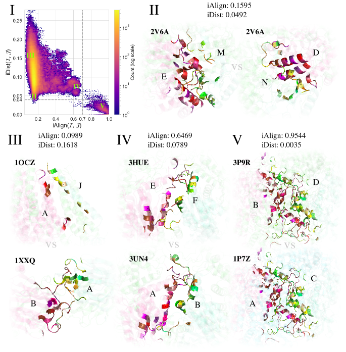
Figure 6: Benchmarking our efficient iDist approximation of the structural alignment algorithm iAlign. (I) Joint log-scale histogram displaying pair-wise iAlign (IS-score mode, $6\mathrm{\mathring{A}}$ cutoff) and iDist values of 1646 PPI interfaces sampled from DIPS (Townshend et al., 2019). The iAlign values vary between 0 and 1, with high values corresponding to well-aligned interfaces (1 for identical interfaces) and low values corresponding to poorly-aligned interfaces. The iDist varies between 0 to infinity with high values corresponding to structurally-distant interfaces and low values corresponding to similar interfaces (0 for identical interfaces). Figures (III, IV, V) depict samples from regions in (I) where the two methods correlate, while (II) shows an example of a disagreement. Each figure displays two interfaces colored by amino acid types, with one protein’s palette in reddish hues and the other one in greenish hues. (II) Ambiguous comparison. The score of iAlign corresponds to the expected value of the alignment of two random PPIs, while iDist suggests high similarity due to the identity of several fragments of chains M and N (note the $\varepsilon$-like green shape and its further continuation) and similar composition of the helices belonging to proteins E and D (similar combination of reddish colors). In fact, the two interfaces represent different interaction modes of the same two chains in a large symmetric complex. (III) Unrelated interfaces. (IV) Interfaces on the edge of being considered near duplicates. The interactions are obviously related, but the geometry and primary structure differ at every local fragment. (V) Near duplicates.

B.1 Implementation details

We implement PPIformer in PyTorch (Paszke et al., 2019) leveraging PyTorch Geometric (Fey & Lenssen, 2019), PyTorch Lightning (Falcon & The PyTorch Lightning team, 2019), Graphein (Jamasb et al., 2020), and a publicly available implementation of Equiformer. We pre-train our model on four AMD MI250X GPUs (8 PyTorch devices) in a distributed data parallel (DDP) mode. Our best model was trained for 32 epochs of dynamic masking in 22 hours.

We pre-train PPIformer by sampling mini-batches of protein–protein interfaces using the Adam optimizer with the default $\beta_{1}=0.9$, $\beta_{2}=0.999$ (Kingma & Ba, 2014). We partially explore the grid of hyper-parameters given by Table 4, and select the best model according to the performance on zero-shot $\Delta\Delta G$ inference on the training set of SKEMPI v2.0. We further fine-tune the model on the same data with the learning rate of $3\cdot 10^{-4}$ and sampling 32 mutations per GPU in a single training step, such that each mutation is from a different PPI. We employ the three-fold cross-validation setup discussed in the next section, and ensemble three corresponding fine-tuned models for test predictions. We observe that dividing $C_{\alpha}$ by 4, as proposed by Watson et al. (2023), increases the rate of convergence.

[]

Table 4: Setting of key pre-training hyper-parameters. The configuration of the best model, referred to as PPIformer, is highlighted in bold.

Category	Hyper-parameter	Values
Data	Dataset	PPIRef50K, PPIRef300K, PPIRef800K,
		DIPS, iDist-deduplicated DIPS
	Num. neighbors $k$	10, 30
		$\mathbf{\{C_{\alpha}\rightarrow C_{\beta}^{virtual}\}}$,
	Type-1 features $\mathbf{F}_{1}$	$\{C_{\alpha}\rightarrow C_{\beta}^{virtual},C_{\alpha}\rightarrow N,C_{\alpha}\rightarrow C\}$,
		$\{C_{\alpha}\rightarrow C_{\beta}^{virtual}C_{\alpha}\rightarrow C_{\alpha}^{prev},C_{\alpha}\rightarrow C_{\alpha}^{next}\}$
Masking	Fraction	$1,15\%,30\%$, $\mathbf{50\%}$
	Same chain	True, False
	$80\%10\%10\%$ BERT masking	True, False
Equiformer	Num. layers $L$	2, 4, 8
	Num. heads $K$	2, 4, 8
	Hidden degree $deg$	1
	Hidden dimensions $\mathbf{d}$	$\mathbf{[128,64]}$
Loss	Label smoothing $\epsilon$	$0,\mathbf{0.1},0.5$
	Class weights $\mathbf{w}$	True, False
Optimization	Learning rate	$1\cdot 10^{-3},\mathbf{5\cdot 10^{-4}},3\cdot 10^{-4},1\cdot 10^{-4}$
	Batch size per GPU	8, 16, 32, 64

B.2 Test datasets

SKEMPI v2.0 split.

In contrast to previous works (Luo et al., 2023; Shan et al., 2022; Liu et al., 2021), we do not create a PDB-disjoint split of SKEMPI v2.0 (based on the #Pdb column) to evaluate the performance of the models. We found that this approach results in at least two kinds of data leakage, limiting the evaluation of generalization towards unseen binders. To illustrate the leakage, we analyze the most recent cross-validation split used to train and test the RDE-Network model (Luo et al., 2023). First, we find that every third test mutation is, in fact, a mutation of the training PPI with a different PDB code in the test set (but with the same Protein 1 and Protein 2 values). Second, more than half of the test PDB codes violate the original hold-out separation proposed by the authors of SKEMPI v2.0. Specifically, Jankauskaitė et al. (2019) performed automated clustering of PPIs followed by manual inspection in order to split the entries into independent groups for the evaluation of machine learning generalization, resulting in the Hold_out_proteins column. We observe that 57% of test PPIs in the PDB-disjoint split in (Luo et al., 2023) violate the proposed grouping, i.e. they have a homologous training PPI, with the same Hold_out_proteins value.

For example, the first two PPIs present in the SKEMPI v2.0 dataset, 1AO7_ABC_DE and 4FTV_ABC_DE, are interactions between the same human T-cell receptor and HLA-A with the viral peptide. These complexes share almost identical 3D structure and are both labeled with the same 6 mutations with slightly different $\Delta\Delta G$ values. As a result, they have identical Protein 1 and Protein 2 values and, consequently, also belong to the same Hold_out_proteins group. Nevertheless, in the RDE-Network split, they are separated into different folds, exemplifying the data leakage in a random PDB-disjoint split.

In contrast, to ensure the effective evaluation of generalization, we split the SKEMPI v2.0 dataset into 3 cross-validation folds based on the Hold_out_proteins feature, as originally proposed by the dataset authors. Additionally, we stratify the $\Delta\Delta G$ distribution across the folds to ensure a balance in labels. Before performing the cross-validation split, we set aside 5 distinct PPIs to form 5 test folds. We consider a PPI distinct if it does not share interacting partners and does not have a homologous binding site (Jankauskaitė et al., 2019) with any other PPI in SKEMPI v2.0 (and, as a result, has a distinct Hold_out_proteins value). Additionally, we ensure that for each of the 5 selected interactions, both negative and positive $\Delta\Delta G$ labels are present. Finally, the maximum iAlign IS-score between all PPIs in the test folds and the cross-validation folds is 0.22, confirming the intended structural independence of the test set. Please refer to Table 5 for details on the constructed test set.

Optimization of a human antibody against SARS-CoV-2.

We utilize the benchmark of Luo et al. (2023) to test the capabilities of the models to optimize a human antibody against SARS-CoV-2. Specifically, the goal is to retrieve 5 mutations on the heavy chain CDR region of the antibody that are known to enhance the neutralization effectiveness within a pool of all exhaustive 494 single-point mutations on the interface.

Engineering staphylokinase for enhanced thrombolytic activity.

We assess the potential of the methods to enhance the thrombolytic activity of the staphylokinase protein (SAK). Staphylokinase, known for its cost-effectiveness and safety as a thrombolytic agent, faces a significant limitation in its widespread clinical application due to its low affinity to plasmin (Nikitin et al., 2022). In this study, we leverage 80 thrombolytic activity labels associated with SAK mutations located at the binding interface with plasmin (Laroche et al., 2000).

Specifically, we evaluate the $\Delta\Delta G$ predictions on the 1BUI structure from PDB, which contains the trimer consisting of plasmin-activated staphylokinase bound to another plasmin substrate. Unlike in the case of the SARS-CoV-2 benchmark, all 80 binary labels for SAK-plasmin have experimentally measured effects, among which 28 mutations are favorable. Additionally, 6 of them introduce at least two-fold thrombolytic activity improvement, constituting even more practically-significant targets for retrieval. Besides that, 24 out of 80 mutations on SAK are multi-point, which provides a more general setup for the evaluation than the SARS-CoV-2 benchmark. Note that while the quantity measured for SAK is the activity, what we are estimating is the $\Delta\Delta G$ for the SAK-plasmin interaction. Since the affinity of the complex is the main activity bottleneck, these two quantities were shown to be highly correlated (Nikitin et al., 2022).

B.3 Evaluation metrics

In a practical binder design scenario (Nikitin et al., 2022; Shan et al., 2022), the primary objectives typically include (i) prioritizing mutations with lower $\Delta\Delta G$ values, and more specifically, (ii) identifying stabilizing mutations (with negative $\Delta\Delta G$) from a pool of candidates. To address (i), we evaluate models using the Spearman correlation coefficient between the ground-truth and predicted $\Delta\Delta G$ values. For (ii), we calculate precision and recall with respect to mutations with negative $\Delta\Delta G$. To enable comparisons with other methods, we also report metrics used in previous work: Pearson correlation coefficient, mean absolute error (MAE), root mean squared error (RMSE), and area under the receiver operating characteristic (ROC AUC). However, we stress that these metrics may be misleading when selecting a model for a practical application. Pearson correlation may not capture the non-linear scoring capabilities of a method and is sensitive to outlying and less significant predictions on destabilizing mutations. MAE and RMSE are not invariant to monotonic transformations of predictions, and ROC AUC may overemphasise the performance on destabilizing mutations. On the independent SARS-CoV-2 and SAK engineering case studies, we report scores for each of the favorable mutations following Luo et al. (2023). In addition, we evaluate more systematic precision at 1 (P@1) and precisions at $k\%$ of the total pool of mutations (P@$k\%$) for $k\in\{5,10\}$.

B.4 Baselines

Flex ddG (Barlow et al., 2018).

Flex ddG is a Rosetta (Leman et al., 2020) protocol which predicts $\Delta\Delta G$ by estimating the change in binding free energies between the wild type and the mutant using force field simulations. For each mutation, the $\Delta\Delta G$ prediction is obtained by averaging the output from 5 runs of ddG-no_backrub_control, a number shown to be optimal by Barlow et al. (2018). Since on average the prediction of a single $\Delta\Delta G$ on the SKEMPI v2.0 test folds using Flex ddG requires approximately 1 CPU hour (on Intel Xeon Gold 6130), we do not evaluate the complete ddG-backrub protocol. When using the ddG-backrub parameters suggested by Barlow et al. (2018), the running time further increases by orders of magnitude, making the method impractical when compared to other baseline methods. For comparison, on the same data where Flex ddG takes on average 1 CPU hour per mutation, our PPIformer requires 73 GPU milliseconds per mutation (using one out of two devices on AMD MI250X GPU with the batch size of 1).

MSA Transformer (Rao et al., 2021).

MSA Transformer is an unsupervised sequence-based baseline, trained in a self-supervised way on diverse multiple sequence alignments (MSA). We use the pre-trained model provided by Rao et al. (2021) and build MSAs against UniRef30 database using HHblits algorithm (Remmert et al., 2012) with the same parameters as were used to train the MSA Transformer. MSA Transformer can be applied to score mutations in a few-shot setup relying on masked pre-training (Meier et al., 2021). More specifically, the $\Delta\Delta G$ can be predicted as a difference of the log-likelihoods of the wild-type and mutant sequences conditioned on a provided MSA.

ESM-IF (Hsu et al., 2022).

ESM-IF, an inverse folding model, has been demonstrated by Hsu et al. (2022) to effectively generalize for predicting the stabilities of SKEMPI complexes upon single-point mutations. To predict $\Delta G$, the authors compute the average log-likelihood of amino acids within a mutated chain, conditioned on the backbone structure of the complex. As done by the authors, to predict $\Delta\Delta G$, we subtract the averaged likelihood of a mutant chain from that of the wildtype chain. Additionally, to account for simultaneous mutations across multiple chains, we perform an ESM-IF forward pass for each chain in a complex and average their likelihoods to obtain the final result.

[]

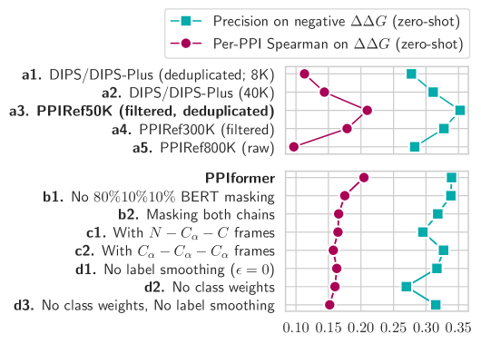
Figure 7: Pre-training ablations with respect to datasets and PPIformer masking strategies, input protein representations, and loss functions. The metrics show zero-shot performance on the training fold of the SKEMPI v2.0 dataset, i.e. $\Delta\Delta G$ inference according to Equation 8 without any supervision. Each row in the Figure represents a single modification of the complete PPIformer model.

RDE-Network (Luo et al., 2023).

For the evaluation on SKEMPI-independent case studies, we use pre-trained model weights as provided by Luo et al. (2023). To validate the performance of RDE-Network on our 5 test folds of SKEMPI v2.0, we exclude all test examples from cross-validation and retrain the model with the same hyperparameters as used by Luo et al. (2023). Since the exclusion of data points affects the sampling of training batches, and may, therefore, negatively affect the performance, we use 3 different random seeds and choose the final model according to the minimal validation loss.

Appendix C Ablations

Self-supervised pre-training.

This section evaluates the effects of the components proposed to enhance the generalization capabilities of PPIformer. First of all, Figure 7 (Top) illustrates that PPIformer achieves a notable performance without any supervised fine-tuning (per-PPI $\rho_{Spearman}=0.21$ and precision = 35% on 5,643 mutations from SKEMPI v2.0). Next, we discuss the importance of the key PPIformer components by analyzing the performance when they change. First of all, the best pre-training is achieved when sampling protein–protein interactions from our PPIRef50K dataset, both on scoring mutations and detecting the stabilizing ones (a3). We observe that training from redundant PPIRef300K decreases the performance, most probably, because of introducing biases towards over-represented proteins and interactions into the model (a4). Finally, training from raw putative PPIs (a5) achieves the worst performance while training from DIPS (a1, a2) or alternatively DIPS-Plus (a1, a2) is still worse than our PPIRef (a3).

[]

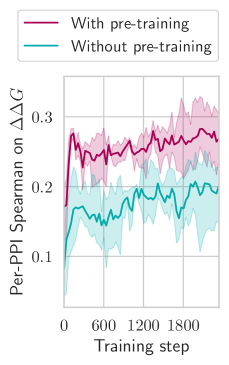
Figure 8: The effect of pre-training on $\Delta\Delta G$ fine-tuning. A training step is performed by sampling a single mutation from each PPI in a randomly sampled batch. The shaded areas correspond to the minimum, mean and maximum of the performance of three models on three-fold cross-validation.

Next, we evaluate the benefits of three key components of PPIformer: masking strategy, data representation and the loss function. First, the $80\%10\%10\%$ masking (i.e. replacing 10% of masked nodes with native amino acids and 10% with random ones (Devlin et al., 2018)) leads to better performance (b1), as well as masking only residues from the same chain (b2), which better corresponds to practical binder design scenarios. Next, as discussed in Section 4.1, we represent the orientations of residues with a single virtual beta-carbon vector per residue. This is in contrast with the more widely adopted utilization of three vectors per residue describing the complete frame of an amino acid by including the direction to a real $C_{\beta}$ and the directions to alpha-carbons of neighboring residues (Jing et al., 2020) or, alternatively, two orthonormalized vectors in the directions of neighboring $N$ and $C$ atoms along the protein backbone (Watson et al., 2023; Yim et al., 2023). We observe that a single virtual beta carbon (used in our PPIformer) leads to better generalization compared to extra full-frame representations (c1, c2). Finally, the regularization by label smoothing and amino acid class weighting have additional strong positive impact on the generalization capabilities of PPIformer. Switching off the regularizations significantly lowers the performance (d1-d3).

Fine-tuning on $\Delta\Delta G$ labels.

We further ablate the importance of our self-supervised pre-training for the $\Delta\Delta G$ fine-tuning. Figure 8 illustrates the crucial significance of the pre-training. The pre-trained PPIformer surpasses the randomly initialized model with a large margin of 0.08 absolute difference on per-PPI Spearman correlation. Note that the pre-trained zero-shot predictor (red curve at step 0) achieves performance competitive to the fully trained model without pre-training (green curve, highest peak).

Appendix D Additional results

In this section, we provide a more detailed comparison of our method with the state-of-the-art approaches on the SKEMPI v2.0 test set. Table 5 demonstrates that, measured by the Spearman correlation coefficient between the predicted and ground-truth $\Delta\Delta G$ values, PPIformer achieves the best or the second-best result on all five protein–protein interactions, outperforming the state-of-the-art methods.

Method	Spearman	Precision	Recall
Flex ddG	0.68	100%	50.00%
MSA Transformer	0.61	100%	100%
ESM-IF	0.34	50.00%	50.00%
RDE-Net.	0.68	100%	100%
PPIformer	0.75	100%	100%

Complement C3d and Fibrinogen-binding protein Efb-C (9 mutations, 4 neg., 5. pos.)

Method	Spearman	Precision	Recall
Flex ddG	0.82	42.86%	42.86%
MSA Transformer	0.43	87.50%	50.00%
ESM-IF	0.60	33.33%	28.57%
RDE-Net.	0.58	42.11%	57.14%
PPIformer	0.60	38.46%	71.43%

Barnase and barnstar (105 mutations, 14 neg., 91 pos.)

Method	Spearman	Precision	Recall
Flex ddG	0.98	100%	100%
MSA Transformer	0.05	66.67%	40.00%
ESM-IF	0.09	0.00%	0.00%
RDE-Net.	0.15	50.00%	40.00%
PPIformer	0.34	60.00%	60.00%

C. thermophilum YTM1–C. and thermophilum ERB1 (10 mutations, 5 neg., 5 pos.)

Method	Spearman	Precision	Recall
Flex ddG	-0.05	29.27%	85.71%
MSA Transformer	-	-	-
ESM-IF	0.38	66.67%	28.57%
RDE-Net.	-0.40	30.23%	92.86%
PPIformer	0.00	53.33%	57.14%

dHP1 Chromodomain and H3 tail (46 mutations, 14 neg., 2 zero, 30 pos.)

Method	Spearman	Precision	Recall
Flex ddG	0.29	44.44%	33.33%
MSA-Transformer	0.37	0.00%	0.00%
ESM-IF	0.21	30.77%	33.33%
RDE-Net.	0.21	50.00%	33.33%
PPIformer	0.43	40%	16.67%

E6AP and UBCH7 (49 mutations, 12 neg., 37 pos.)

Table 5: Performance of PPIformer and other competitive methods on 5 held-out test cases from SKEMPI v2.0. MSA Transformer is not evaluated on the “dHP1 Chromodomain and H3 tail” test case because HHblits outputs an empty MSA for the short binding peptide of 8 amino acids.

References

- Barlow et al. (2018) Kyle A. Barlow, Shane Ó Conchúir, Samuel Thompson, Pooja Suresh, James E. Lucas, Markus Heinonen, and Tanja Kortemme. Flex ddg: Rosetta ensemble-based estimation of changes in protein–protein binding affinity upon mutation. The Journal of Physical Chemistry B, 122(21):5389–5399, May 2018. ISSN 1520-6106. doi: 10.1021/acs.jpcb.7b11367. URL https://doi.org/10.1021/acs.jpcb.7b11367.
- Berman et al. (2000) Helen M Berman, John Westbrook, Zukang Feng, Gary Gilliland, Talapady N Bhat, Helge Weissig, Ilya N Shindyalov, and Philip E Bourne. The protein data bank. Nucleic acids research, 28(1):235–242, 2000.
- Burra et al. (2009) Prasad V Burra, Ying Zhang, Adam Godzik, and Boguslaw Stec. Global distribution of conformational states derived from redundant models in the pdb points to non-uniqueness of the protein structure. Proceedings of the National Academy of Sciences, 106(26):10505–10510, 2009. URL https://doi.org/10.1073/pnas.081215210.
- Cheng et al. (2015) Shanshan Cheng, Yang Zhang, and Charles L Brooks. Pcalign: a method to quantify physicochemical similarity of protein-protein interfaces. BMC bioinformatics, 16(1):1–12, 2015.
- Dauparas et al. (2022) Justas Dauparas, Ivan Anishchenko, Nathaniel Bennett, Hua Bai, Robert J Ragotte, Lukas F Milles, Basile IM Wicky, Alexis Courbet, Rob J de Haas, Neville Bethel, et al. Robust deep learning–based protein sequence design using proteinmpnn. Science, 378(6615):49–56, 2022.
- Dehouck et al. (2013) Yves Dehouck, Jean Marc Kwasigroch, Marianne Rooman, and Dimitri Gilis. Beatmusic: prediction of changes in protein–protein binding affinity on mutations. Nucleic acids research, 41(W1):W333–W339, 2013.
- Devlin et al. (2018) Jacob Devlin, Ming-Wei Chang, Kenton Lee, and Kristina Toutanova. Bert: Pre-training of deep bidirectional transformers for language understanding. arXiv preprint arXiv:1810.04805, 2018.
- Draizen et al. (2022) Eli J. Draizen, Luis Felipe R. Murillo, John Readey, Cameron Mura, and Philip E. Bourne. Prop3d: A flexible, python-based platform for machine learning with protein structural properties and biophysical data. bioRxiv, 2022. doi: 10.1101/2022.12.27.522071. URL https://www.biorxiv.org/content/early/2022/12/30/2022.12.27.522071.
- Evans et al. (2021) Richard Evans, Michael O’Neill, Alexander Pritzel, Natasha Antropova, Andrew Senior, Tim Green, Augustin Žídek, Russ Bates, Sam Blackwell, Jason Yim, et al. Protein complex prediction with alphafold-multimer. biorxiv, pp. 2021–10, 2021.
- Falcon & The PyTorch Lightning team (2019) William Falcon and The PyTorch Lightning team. PyTorch Lightning, mar 2019. URL https://github.com/Lightning-AI/lightning.
- Feigin et al. (2022) Valery L Feigin, Michael Brainin, Bo Norrving, Sheila Martins, Ralph L Sacco, Werner Hacke, Marc Fisher, Jeyaraj Pandian, and Patrice Lindsay. World stroke organization (wso): global stroke fact sheet 2022. International Journal of Stroke, 17(1):18–29, 2022.
- Fey & Lenssen (2019) Matthias Fey and Jan Eric Lenssen. Fast graph representation learning with pytorch geometric. arXiv preprint arXiv:1903.02428, 2019.
- Gainza et al. (2020) Pablo Gainza, Freyr Sverrisson, Frederico Monti, Emanuele Rodola, D Boscaini, MM Bronstein, and BE Correia. Deciphering interaction fingerprints from protein molecular surfaces using geometric deep learning. Nature Methods, 17(2):184–192, 2020.
- Gainza et al. (2023) Pablo Gainza, Sarah Wehrle, Alexandra Van Hall-Beauvais, Anthony Marchand, Andreas Scheck, Zander Harteveld, Stephen Buckley, Dongchun Ni, Shuguang Tan, Freyr Sverrisson, et al. De novo design of protein interactions with learned surface fingerprints. Nature, pp. 1–9, 2023.
- Ganea et al. (2021) Octavian-Eugen Ganea, Xinyuan Huang, Charlotte Bunne, Yatao Bian, Regina Barzilay, Tommi Jaakkola, and Andreas Krause. Independent se (3)-equivariant models for end-to-end rigid protein docking. arXiv preprint arXiv:2111.07786, 2021.
- Gao & Skolnick (2010a) Mu Gao and Jeffrey Skolnick. ialign: a method for the structural comparison of protein–protein interfaces. Bioinformatics, 26(18):2259–2265, 2010a. URL https://doi.org/10.1093/bioinformatics/btq404.
- Gao & Skolnick (2010b) Mu Gao and Jeffrey Skolnick. Structural space of protein–protein interfaces is degenerate, close to complete, and highly connected. Proceedings of the National Academy of Sciences, 107(52):22517–22522, 2010b. URL 10.1073/pnas.1012820107.
- Geng et al. (2019a) Cunliang Geng, Anna Vangone, Gert E Folkers, Li C Xue, and Alexandre MJJ Bonvin. isee: Interface structure, evolution, and energy-based machine learning predictor of binding affinity changes upon mutations. Proteins: Structure, Function, and Bioinformatics, 87(2):110–119, 2019a.
- Geng et al. (2019b) Cunliang Geng, Li C Xue, Jorge Roel-Touris, and Alexandre MJJ Bonvin. Finding the g spot: Are predictors of binding affinity changes upon mutations in protein–protein interactions ready for it? Wiley Interdisciplinary Reviews: Computational Molecular Science, 9(5):e1410, 2019b.
- Hsu et al. (2022) Chloe Hsu, Robert Verkuil, Jason Liu, Zeming Lin, Brian Hie, Tom Sercu, Adam Lerer, and Alexander Rives. Learning inverse folding from millions of predicted structures. bioRxiv, 2022. doi: 10.1101/2022.04.10.487779.
- Ivanov et al. (2013) Andrei A Ivanov, Fadlo R Khuri, and Haian Fu. Targeting protein–protein interactions as an anticancer strategy. Trends in pharmacological sciences, 34(7):393–400, 2013.
- Jamasb et al. (2020) Arian R Jamasb, Ramon Viñas, Eric J Ma, Charlie Harris, Kexin Huang, Dominic Hall, Pietro Lió, and Tom L Blundell. Graphein-a python library for geometric deep learning and network analysis on protein structures and interaction networks. bioRxiv, pp. 2020–07, 2020.
- Jankauskaitė et al. (2019) Justina Jankauskaitė, Brian Jiménez-García, Justas Dapkūnas, Juan Fernández-Recio, and Iain H Moal. Skempi 2.0: an updated benchmark of changes in protein–protein binding energy, kinetics and thermodynamics upon mutation. Bioinformatics, 35(3):462–469, 2019.
- Jin et al. (2023) Wengong Jin, Siranush Sarkizova, Xun Chen, Nir Hacohen, and Caroline Uhler. Unsupervised protein-ligand binding energy prediction via neural euler’s rotation equation. arXiv preprint arXiv:2301.10814, 2023.
- Jing et al. (2020) Bowen Jing, Stephan Eismann, Patricia Suriana, Raphael JL Townshend, and Ron Dror. Learning from protein structure with geometric vector perceptrons. arXiv preprint arXiv:2009.01411, 2020.
- Jumper et al. (2021) John Jumper, Richard Evans, Alexander Pritzel, Tim Green, Michael Figurnov, Olaf Ronneberger, Kathryn Tunyasuvunakool, Russ Bates, Augustin Žídek, Anna Potapenko, et al. Highly accurate protein structure prediction with alphafold. Nature, 596(7873):583–589, 2021.
- Karniadakis et al. (2021) George Em Karniadakis, Ioannis G Kevrekidis, Lu Lu, Paris Perdikaris, Sifan Wang, and Liu Yang. Physics-informed machine learning. Nature Reviews Physics, 3(6):422–440, 2021.
- Kastritis & Bonvin (2013) Panagiotis L Kastritis and Alexandre MJJ Bonvin. On the binding affinity of macromolecular interactions: daring to ask why proteins interact. Journal of The Royal Society Interface, 10(79):20120835, 2013.
- Ketata et al. (2023) Mohamed Amine Ketata, Cedrik Laue, Ruslan Mammadov, Hannes Stärk, Menghua Wu, Gabriele Corso, Céline Marquet, Regina Barzilay, and Tommi S Jaakkola. Diffdock-pp: Rigid protein-protein docking with diffusion models. arXiv preprint arXiv:2304.03889, 2023.
- Kingma & Ba (2014) Diederik P Kingma and Jimmy Ba. Adam: A method for stochastic optimization. arXiv preprint arXiv:1412.6980, 2014.
- Langan et al. (2019) Robert A Langan, Scott E Boyken, Andrew H Ng, Jennifer A Samson, Galen Dods, Alexandra M Westbrook, Taylor H Nguyen, Marc J Lajoie, Zibo Chen, Stephanie Berger, et al. De novo design of bioactive protein switches. Nature, 572(7768):205–210, 2019.
- Laroche et al. (2000) Yves Laroche, Stephane Heymans, Sophie Capaert, Frans De Cock, Eddy Demarsin, and Désiré Collen. Recombinant staphylokinase variants with reduced antigenicity due to elimination of b-lymphocyte epitopes. Blood, The Journal of the American Society of Hematology, 96(4):1425–1432, 2000.
- Leman et al. (2020) Julia Koehler Leman, Brian D Weitzner, Steven M Lewis, Jared Adolf-Bryfogle, Nawsad Alam, Rebecca F Alford, Melanie Aprahamian, David Baker, Kyle A Barlow, Patrick Barth, et al. Macromolecular modeling and design in rosetta: recent methods and frameworks. Nature methods, 17(7):665–680, 2020.
- Liao & Smidt (2022) Yi-Lun Liao and Tess Smidt. Equiformer: Equivariant graph attention transformer for 3d atomistic graphs. arXiv preprint arXiv:2206.11990, 2022.
- Liao et al. (2023) Yi-Lun Liao, Brandon Wood, Abhishek Das, and Tess Smidt. Equiformerv2: Improved equivariant transformer for scaling to higher-degree representations. arXiv preprint arXiv:2306.12059, 2023.
- Lin et al. (2023) Zeming Lin, Halil Akin, Roshan Rao, Brian Hie, Zhongkai Zhu, Wenting Lu, Nikita Smetanin, Robert Verkuil, Ori Kabeli, Yaniv Shmueli, et al. Evolutionary-scale prediction of atomic-level protein structure with a language model. Science, 379(6637):1123–1130, 2023.
- Liu et al. (2021) Xianggen Liu, Yunan Luo, Pengyong Li, Sen Song, and Jian Peng. Deep geometric representations for modeling effects of mutations on protein-protein binding affinity. PLoS computational biology, 17(8):e1009284, 2021.
- Lu et al. (2020) Haiying Lu, Qiaodan Zhou, Jun He, Zhongliang Jiang, Cheng Peng, Rongsheng Tong, and Jianyou Shi. Recent advances in the development of protein–protein interactions modulators: mechanisms and clinical trials. Signal transduction and targeted therapy, 5(1):213, 2020.
- Luo et al. (2023) Shitong Luo, Yufeng Su, Zuofan Wu, Chenpeng Su, Jian Peng, and Jianzhu Ma. Rotamer density estimator is an unsupervised learner of the effect of mutations on protein-protein interaction. In The Eleventh International Conference on Learning Representations, 2023. URL https://openreview.net/forum?id=_X9Yl1K2mD.
- Marchand et al. (2022) Anthony Marchand, Alexandra K Van Hall-Beauvais, and Bruno E Correia. Computational design of novel protein–protein interactions–an overview on methodological approaches and applications. Current Opinion in Structural Biology, 74:102370, 2022.
- Meier et al. (2021) Joshua Meier, Roshan Rao, Robert Verkuil, Jason Liu, Tom Sercu, and Alex Rives. Language models enable zero-shot prediction of the effects of mutations on protein function. Advances in Neural Information Processing Systems, 34:29287–29303, 2021.
- Mirabello & Wallner (2018) Claudio Mirabello and Björn Wallner. Topology independent structural matching discovers novel templates for protein interfaces. Bioinformatics, 34(17):i787–i794, 2018. doi: 10.1093/bioinformatics/bty587.
- Morehead et al. (2021) Alex Morehead, Chen Chen, Ada Sedova, and Jianlin Cheng. Dips-plus: The enhanced database of interacting protein structures for interface prediction. arXiv preprint arXiv:2106.04362, 2021.
- Nikitin et al. (2022) Dmitri Nikitin, Jan Mican, Martin Toul, David Bednar, Michaela Peskova, Patricia Kittova, Sandra Thalerova, Jan Vitecek, Jiri Damborsky, Robert Mikulik, et al. Computer-aided engineering of staphylokinase toward enhanced affinity and selectivity for plasmin. Computational and structural biotechnology journal, 20:1366–1377, 2022.
- Pahari et al. (2020) Swagata Pahari, Gen Li, Adithya Krishna Murthy, Siqi Liang, Robert Fragoza, Haiyuan Yu, and Emil Alexov. Saambe-3d: predicting effect of mutations on protein–protein interactions. International journal of molecular sciences, 21(7):2563, 2020.
- Paszke et al. (2019) Adam Paszke, Sam Gross, Francisco Massa, Adam Lerer, James Bradbury, Gregory Chanan, Trevor Killeen, Zeming Lin, Natalia Gimelshein, Luca Antiga, et al. Pytorch: An imperative style, high-performance deep learning library. Advances in neural information processing systems, 32, 2019.
- Rao et al. (2021) Roshan M Rao, Jason Liu, Robert Verkuil, Joshua Meier, John Canny, Pieter Abbeel, Tom Sercu, and Alexander Rives. Msa transformer. In International Conference on Machine Learning, pp. 8844–8856. PMLR, 2021.
- Remmert et al. (2012) Michael Remmert, Andreas Biegert, Andreas Hauser, and Johannes Söding. Hhblits: lightning-fast iterative protein sequence searching by hmm-hmm alignment. Nature Methods, 9(2):173–175, Feb 2012. ISSN 1548-7105. doi: 10.1038/nmeth.1818. URL https://doi.org/10.1038/nmeth.1818.
- Ribeiro et al. (2019) Judemir Ribeiro, Carlos Ríos-Vera, Francisco Melo, and Andreas Schüller. Calculation of accurate interatomic contact surface areas for the quantitative analysis of non-bonded molecular interactions. Bioinformatics, 35(18):3499–3501, 2019.
- Rives et al. (2021) Alexander Rives, Joshua Meier, Tom Sercu, Siddharth Goyal, Zeming Lin, Jason Liu, Demi Guo, Myle Ott, C Lawrence Zitnick, Jerry Ma, et al. Biological structure and function emerge from scaling unsupervised learning to 250 million protein sequences. Proceedings of the National Academy of Sciences, 118(15):e2016239118, 2021.
- Rodrigues et al. (2021) Carlos HM Rodrigues, Douglas EV Pires, and David B Ascher. mmcsm-ppi: predicting the effects of multiple point mutations on protein–protein interactions. Nucleic Acids Research, 49(W1):W417–W424, 2021.
- Scheller et al. (2018) Leo Scheller, Tobias Strittmatter, David Fuchs, Daniel Bojar, and Martin Fussenegger. Generalized extracellular molecule sensor platform for programming cellular behavior. Nature chemical biology, 14(7):723–729, 2018.
- Schymkowitz et al. (2005) Joost Schymkowitz, Jesper Borg, Francois Stricher, Robby Nys, Frederic Rousseau, and Luis Serrano. The foldx web server: an online force field. Nucleic acids research, 33(suppl_2):W382–W388, 2005.
- Shan et al. (2022) Sisi Shan, Shitong Luo, Ziqing Yang, Junxian Hong, Yufeng Su, Fan Ding, Lili Fu, Chenyu Li, Peng Chen, Jianzhu Ma, et al. Deep learning guided optimization of human antibody against sars-cov-2 variants with broad neutralization. Proceedings of the National Academy of Sciences, 119(11):e2122954119, 2022.
- Shin et al. (2023a) Woong-Hee Shin, Keiko Kumazawa, Kenichiro Imai, Takatsugu Hirokawa, and Daisuke Kihara. Quantitative comparison of protein-protein interaction interface using physicochemical feature-based descriptors of surface patches. Frontiers in Molecular Biosciences, 10, 2023a. URL https://doi.org/10.3389/fmolb.2023.1110567.
- Shin et al. (2023b) Woong-Hee Shin, Keiko Kumazawa, Kenichiro Imai, Takatsugu Hirokawa, and Daisuke Kihara. Quantitative comparison of protein-protein interaction interface using physicochemical feature-based descriptors of surface patches. Frontiers in Molecular Biosciences, 10:1110567, 2023b.
- Shroff et al. (2019) Raghav Shroff, Austin W Cole, Barrett R Morrow, Daniel J Diaz, Isaac Donnell, Jimmy Gollihar, Andrew D Ellington, and Ross Thyer. A structure-based deep learning framework for protein engineering. bioRxiv, pp. 833905, 2019.
- Sora et al. (2023) Valentina Sora, Adrian Otamendi Laspiur, Kristine Degn, Matteo Arnaudi, Mattia Utichi, Ludovica Beltrame, Dayana De Menezes, Matteo Orlandi, Ulrik Kristoffer Stoltze, Olga Rigina, Peter Wad Sackett, Karin Wadt, Kjeld Schmiegelow, Matteo Tiberti, and Elena Papaleo. Rosettaddgprediction for high-throughput mutational scans: From stability to binding. Protein Science, 32(1):e4527, 2023. doi: https://doi.org/10.1002/pro.4527. URL https://onlinelibrary.wiley.com/doi/abs/10.1002/pro.4527.
- Steinegger & Söding (2017) Martin Steinegger and Johannes Söding. Mmseqs2 enables sensitive protein sequence searching for the analysis of massive data sets. Nature biotechnology, 35(11):1026–1028, 2017.
- Szegedy et al. (2016) Christian Szegedy, Vincent Vanhoucke, Sergey Ioffe, Jon Shlens, and Zbigniew Wojna. Rethinking the inception architecture for computer vision. In Proceedings of the IEEE conference on computer vision and pattern recognition, pp. 2818–2826, 2016.
- Townshend et al. (2019) Raphael Townshend, Rishi Bedi, Patricia Suriana, and Ron Dror. End-to-end learning on 3d protein structure for interface prediction. Advances in Neural Information Processing Systems, 32, 2019. URL https://doi.org/10.48550/arXiv.1807.01297.
- van Kempen et al. (2023) Michel van Kempen, Stephanie S Kim, Charlotte Tumescheit, Milot Mirdita, Jeongjae Lee, Cameron LM Gilchrist, Johannes Söding, and Martin Steinegger. Fast and accurate protein structure search with foldseek. Nature Biotechnology, pp. 1–4, 2023. doi: https://doi.org/10.1038/s41587-023-01773-0.
- Vreven et al. (2015) Thom Vreven, Iain H Moal, Anna Vangone, Brian G Pierce, Panagiotis L Kastritis, Mieczyslaw Torchala, Raphael Chaleil, Brian Jiménez-García, Paul A Bates, Juan Fernandez-Recio, et al. Updates to the integrated protein–protein interaction benchmarks: docking benchmark version 5 and affinity benchmark version 2. Journal of molecular biology, 427(19):3031–3041, 2015.
- Wang et al. (2020) Menglun Wang, Zixuan Cang, and Guo-Wei Wei. A topology-based network tree for the prediction of protein–protein binding affinity changes following mutation. Nature Machine Intelligence, 2(2):116–123, 2020.
- Watson et al. (2023) Joseph L Watson, David Juergens, Nathaniel R Bennett, Brian L Trippe, Jason Yim, Helen E Eisenach, Woody Ahern, Andrew J Borst, Robert J Ragotte, Lukas F Milles, et al. De novo design of protein structure and function with rfdiffusion. Nature, pp. 1–3, 2023.
- Xiong et al. (2017) Peng Xiong, Chengxin Zhang, Wei Zheng, and Yang Zhang. Bindprofx: assessing mutation-induced binding affinity change by protein interface profiles with pseudo-counts. Journal of molecular biology, 429(3):426–434, 2017.
- Yim et al. (2023) Jason Yim, Brian L Trippe, Valentin De Bortoli, Emile Mathieu, Arnaud Doucet, Regina Barzilay, and Tommi Jaakkola. Se (3) diffusion model with application to protein backbone generation. arXiv preprint arXiv:2302.02277, 2023.
- Zhang & Skolnick (2004) Yang Zhang and Jeffrey Skolnick. Scoring function for automated assessment of protein structure template quality. Proteins: Structure, Function, and Bioinformatics, 57(4):702–710, 2004.
- Zhang et al. (2023) Zuobai Zhang, Minghao Xu, Vijil Chenthamarakshan, Aurélie Lozano, Payel Das, and Jian Tang. Enhancing protein language models with structure-based encoder and pre-training. arXiv preprint arXiv:2303.06275, 2023.