Differentiable Simulator For Dynamic & Stochastic Optimal Gas & Power Flows

Abstract

In many power systems, particularly those isolated from larger intercontinental grids, operational dependence on natural gas becomes pivotal, especially during fluctuations or unavailability of renewables coupled with uncertain consumption patterns. Efficient orchestration and inventive strategies are imperative for the smooth functioning of these standalone gas-grid systems. This paper delves into the challenge of synchronized dynamic and stochastic optimization for independent transmission-level gas-grid systems. Our approach’s novelty lies in amalgamating the staggered-grid method for the direct assimilation of gas-flow PDEs with an automated sensitivity analysis facilitated by SciML/Julia, further enhanced by an intuitive linkage between gas and power grids via nodal flows. We initiate with a single pipe to establish a versatile and expandable methodology, later showcasing its effectiveness with increasingly intricate examples.

1 Introduction & Background

The increasing penetration of renewable energy sources has amplified unpredictable fluctuations, leading to more severe and uncertain ramps in the duck curve associated with power demand. Simultaneously the transition from coal to cleaner “bridge fuels” such as natural gas, shift even more responsibility to the natural gas system. Beyond power generation, transmission level gas systems face potential stressors from factors such as residential and commercial distribution, and exports. The differing timescales between the gas and power networks — power systems stabilize within seconds and gas systems might take days — complicate coordination efforts in both real-time operations and day-ahead planning across sectors. Previous studies, such as [1] and [2], integrated gas dynamics into day-ahead plans using an optimization framework. These optimizations incorporated constraints for the gas network arising from either steady-state approximations or a coarse discretization of the elliptic approximation to the isothermal gas equations. Recent work has designed linear approximations for pipe segments, trading an increase in computational efficiency with a decrease in fidelity; suitable for integration into optimization frameworks [3]. However, addressing the intrinsic nonlinearity of gas system dynamics, particularly under stressed and uncertain conditions, remains a substantial challenge.

The challenge at hand can be formally articulated as the solution to a PDE-constrained optimization problem, depicted schematically as:

$$\min\limits_{\{u^{(s)}(t),q^{(s)}(t)\}}\sum_{s\in\mathcal{S}}\int_{0}^{T}C^{(s)}(u^{(s)}(t),q^{(s)}(t))\,dt,$$ (1)

$$\hskip 5.69046pt\text{s.t.}\ \forall s,\ \forall t:\ \text{PDE}^{(s)}(u^{(s)}(t),q^{(s)}(t))=0,$$

where $u^{(s)}(t)$ and $q^{(s)}(t)$ signify the time-evolving state space and control degrees of freedom for scenarios or samples $s\in\mathcal{S}$ respectively. The term $C^{(s)}(u^{(s)}(t),q^{(s)}(t))$ denotes the cumulative cost. In our chosen framework: $q^{(s)}(t)$ embodies the gas extraction from the system, which can be redistributed across various nodes of the gas-grid where gas generators are positioned; $u^{(s)}(t)$ represents the gas flows, gas densities, and, indirectly via the gas equation of state, pressures over the gas-grid pipes. The cost function $C^{(s)}(u^{(s)}(t),q^{(s)}(t))$ encapsulates the discrepancy between aggregated energy generation (directly related to gas extraction at nodes) and demand, operational costs of gas generators, and pressure constraints at the gas-grid nodes. The equation $\text{PDE}^{(s)}(u^{(s)}(t),q^{(s)}(t))=0$ characterizes the gas-flow equations, elucidating for each scenario $s$ how gas flows and densities are spatially (across the gas-grid network) and temporally distributed, contingent on the profile of gas extraction and injection. A detailed explanation is provided in Section 2.

In this paper, we propose a novel approach to solving Eq. (1), aiming to enhance the fidelity of gas accounting in day-ahead planning of power generation in a computationally efficient manner. Our solution crafts a differentiable simulator by leveraging the principles of differentiable programming (DP) [4], combined with an efficient explicit staggered-grid method [5], and the robust capabilities of the SciML sensitivity ecosystem [6]. As we delve further, it will become evident that our approach adeptly addresses the intertwined challenges of nonlinearity, dimensionality, and stochastic modeling.

In the proposed framework, differentiable programming facilitates the calculation of gradients by seamlessly solving the gas-flow PDE across a network. This is realized by auto-generating the corresponding adjoint equations, providing flexibility in formulating the forward pass. The approach not only supports sensitivity analysis but, with a judicious selection of algorithms, proficiently manages scalability issues in parameter spaces, all while preserving the intricate nonlinear dynamics.

Driven by the everyday operational challenges characteristic of Israel’s power system, as expounded in [7] and its associated references, we design and solve a dynamic, stochastic problem that integrates power and gas flows over an operational timeframe ranging from several hours to an entire day. We predominantly target smaller, transmission-level systems akin to Israel’s, characterized by:

• Limited availability or operational restrictions of gas compressors;

• Notable fluctuations in renewable resources and power loads, with curtailment being inadmissible under the normal operational paradigms assumed in this research;

• An intentionally overengineered power system, ensuring power lines remain within thermal boundaries during standard operations.

To demonstrate the efficacy of our methodology, we initiate with a single-pipe scenario, advancing thereafter to a more intricate, albeit representative, network.

The remainder of the manuscript is structured as follows: In Section 2, we elucidate our gas modeling methodology, starting with a single pipe before extending to a broader network. Within this section, we also elaborate on our fundamental optimization problem and delineate our strategy for its resolution. Subsequent discussions of our experimental results are presented in Section 3. Finally, the manuscript culminates with conclusions and suggested future directions in Section 4.

2 Methodology

2.1 Gas-Flow Equations

We begin by discussing the dynamics of a single pipe. The governing partial differential equations (PDEs) for the Gas Flow (GF), describing the dynamics of density $\rho(x,t)$ and mass-flux $\phi(x,t)$ along the pipe coordinate $x$ with respect to time $t$, are provided as follows [8],[9]:

$$\partial_{t}\rho+\partial_{x}\phi=0,$$ (2)

$$\partial_{t}\phi+\partial_{x}p=-\frac{\lambda}{2D}\frac{\phi|\phi|}{\rho}.$$ (3)

These equations are valid under the assumption that the gas velocity is much smaller than the speed of sound in the gas ($\phi/\rho\ll a$). This is a reasonable approximation for the typical flows we consider.

To provide a complete description, it is necessary to relate the pressure $p(x,t)$ and density $\rho(x,t)$ using an equation of state:

$$p=Z(\rho,T)RT\rho,$$ (4)

where $Z(\rho,T)$ denotes the compressibility factor. For clarity, we adopt the ideal gas law to model the equation of state, where $Z(\rho,T)RT$ is replaced by a constant, $a^{2}$, with $a$ representing the speed of sound in the gas. Notably, there are more accurate models available (e.g., CNGA [10]), and the methodology we present here is agnostic to the specific choice of model.

The system of Eqs. (2,3,4) is also supplemented by the boundary conditions, for example given profile of injection/consumption, at both ends of the pipe of length $l$, $q(0,t)$ and $q(L,t)$.

To extend the described equations from a single pipe to a network, we must augment the PDEs (2), (3) and equation of state (4) for each pipe with boundary conditions that couple multiple pipes, and work with prescribed injection/consumption at nodes of the network. These numerical details are described in the next section.

2.2 Explicit Numerical Method for the Forward Path

To solve Eqs. (2,3,4) in the case of a single pipe and their network generalizations in more general setting of the PDEs over networks, we use an explicit, second-order, staggered-grid method introduced by Gyrya & Zlotnik [5]. This method applied to the interior of a pipe is shown schematically in Fig. (1). First-order differences in space and time become centered differences due to the variable staggering. In particular, the states $\rho_{i}^{n}:=\rho(x_{i},t_{n})$, $\phi_{j}^{m}:=\phi(x_{j},t_{m})$ (where $i$ and $n$ stand for discretization indexes in time and space, respectively, $m=n+1/2$ and $j=i+1/2$) are advanced in time and space following

$$\rho_{i}^{n+1} =\rho_{i}^{n}-\frac{\Delta t}{\Delta x}\left(\phi_{j}^{m}-\phi_{j-1}^{m}\right),$$ (5)

$$\phi_{j}^{m+1} =\phi_{j}^{m}-\Delta t\left(\frac{p^{n+1}_{i+1}-p^{n+1}_{i}}{\Delta x}+\frac{\lambda}{2D}\frac{\phi^{n+1}_{j}|\phi^{n+1}_{j}|}{\rho_{j}^{n+1}}\right).$$ (6)

Here Eq. (6) is in fact implicit in $\phi_{j}^{m+1}$ due to averaging required to approximate $\phi_{j}^{n+1}$, but an exact solution is available, (see [5] for details). As we are interested in integration in day-ahead planning of energy generation, we control Dirichlet boundary conditions on nodal mass flows $\{q_{i}\}_{i\in\text{nodes}}$ (directly relating to generated power). These boundaries are resolved according to the numerical method using a boundary discretization shown in Fig. (2). The pressure updates for these junctions are evaluated using conservation of mass, and the Kirchoff-Neumann conditions for an update rule for boundary node $\ell$

$$\begin{split}\sum_{k\in\partial\ell}&\frac{\Delta x}{\Delta t}S_{kl}\rho^{n+1}_{\ell}=\\ &q_{l}+\sum_{k\in\partial\ell}\frac{\Delta x}{\Delta t}S_{kl}\rho_{kl}^{n}-\sum_{k\in\partial\ell}\text{sgn}_{kl}S_{kl}\phi_{kl}^{m},\end{split}$$ (7)

where $S_{kl}$ is the cross-section area of pipe from node $k$ to node $l$, and $\text{sgn}_{kl}$ keeps track of the directionality of the mass flux. $\rho_{kl},\phi_{kl}$ denote the $l$-side boundary values of density and mass flux for the pipe from node $k$ to node $l$. After solving for the density at the node, the flux update at the ends of the pipes can proceed using the momentum equation (6).

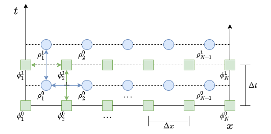
Figure 1: The staggered grid method of [5] uses centered differences on grids offset by $\Delta x/2$ and $\Delta t/2$ to achieve a conservative 2nd-order numerical method for the effective gas-flow equations Eqs. (2-3)

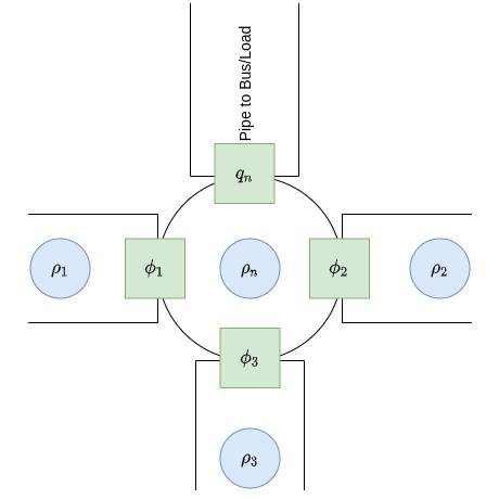
Figure 2: An example of a 3-pipe junction discretization, with a fictitious pipe setting the nodal flow boundary condition.

2.3 Optimization Formulation: Cost Function

In our pursuit to devise a scalable framework that aptly accommodates optimization challenges akin to the archetype presented in Eq. (1), we pivot our attention to a paradigmatic problem: the minimization of an integrated objective spanning time and evaluated under the cloak of uncertainty. This uncertainty, reflected through diverse scenarios $s\in\mathcal{S}$, pertains to the gas injection consumption $q^{(s)}(t):=\{q_{i}^{(s)}(t)\}_{\forall i\in\text{nodes}}$, influenced possibly by variable renewable generation. The time interval $t\in[0,T]$ typically encapsulates a pre-established performance window, like 24 hours.

Our control parameters, symbolized by nodal flows $q^{(s)}(t)$, permit adjustments within our forthcoming dynamic and stochastic optimization context. By solving Eqs. (2-3) for each scenario, we determine the network’s state $u^{(s)}(t):=\{\rho^{(s)}(x,t),\phi^{(s)}(x,t)\}_{\forall x\in\text{nodes \& pipes}}$. To streamline notation, we represent aggregated degrees of freedom over time and scenarios by $u(t):=\{u^{(s)}(x,t)\}_{\forall x\in\text{pipes};\forall s}$ and $q(t):=\{q_{i}^{(s)}(t)\}_{\forall i\in\text{nodes};\forall s}$. Additionally, we define $u:=\{u(t)\}_{\forall t}$ and $q:=\{q(t)\}_{\forall t}$ to aggregate over time.

Our primary optimization task is delineated as minimization of

$$O(u,q)=\sum_{s\in\mathcal{S}}\int_{0}^{T}C^{(s)}(u^{(s)}(t),q^{s}(t))\,dt,$$ (8)

where the specific per-time and per-scenario cost is expanded as:

$$C^{(s)}(u^{(s)} (t),q^{(s)}(t))=\alpha\left(D^{(s)}(t)-\sum_{i\in\text{nodes}}G_{i}(q^{(s)}_{i}(t))\right)^{2}$$ (9)

$$+\beta\sum_{i\in\text{nodes}}E^{(s)}_{i}(q^{(s)}_{i}(t))+\gamma\sum_{x\in\text{nodes}}V(p^{(s)}(x,t)),$$

constrained by the gas-flow PDEs and associated boundary conditions over gas-grid network detailed earlier.

The first term in Eq. (9) aims to minimize the cumulative mismatch between energy demand $D^{(s)}(t)$ and the sum of generation at each node $i$ and at each moment of time $t$, $G_{i}(q^{(s)}_{i}(t))$, with $q_{i}^{(s)}(t)$ representing the nodal flows, which is our control variable (one we are optimizing over). $G_{i}(q^{(s)}_{i}(t))$ is an efficiency function, mapping mass flow (in $kg/s$) to power production (in $MW$). Here the assumption is that any residual mismatch, if not optimal, can be adjusted by either shedding demand or introducing a generation reserve, at a certain cost. The second term in Eq. (9), $E^{(s)}_{i}(q_{i}(t))$, stands for the cost of operating power generator run on gas and located at the node $i$ at the gas withdrawal rate $q_{i}(t)$. The third term in Eq. (9), $\sum_{x\in\text{nodes}}V(p^{(s)}(x,t))$, is chosen to be a quasi-quadratic cost (regularized by the relu function) to penalize pressure constraint violations across the network (refer to Fig. 3): with $p_{\text{min}}(x)$ and $p_{\text{max}}(x)$ denoting pre-set pressure boundaries at system nodes. The influence of $C^{(s)}$’s components can be modulated using the hyperparameters $\alpha$, $\beta$, and $\gamma$.

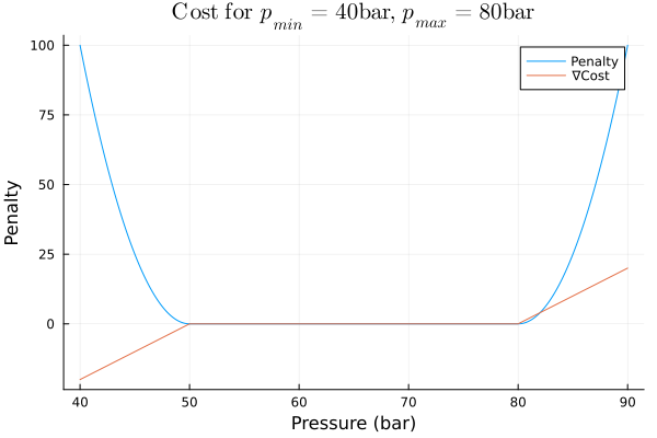
Figure 3: Quasi-quadratic penalty for violating pressure constraints, with $40-80$ bar shown here, but configurable on a per-node basis.

2.4 Solving PDE Constrained Optimization

In this Section, we elucidate our strategy to address Eq. (1). Essentially, two predominant methodologies emerge for tackling the PDE-constrained optimization challenge:

1. Constraint Matrix Encoding: This method integrates the PDE into a constraint matrix that grows as discretization becomes finer. A notable merit of this approach is its flexibility in harnessing advanced optimization techniques. On the flip side, the methodology grapples with potential pitfalls such as the emergence of unphysical solutions, non-adherence to constraints during intermediary timeframes, and the curse of dimensionality, manifesting as an exponential surge in complexity with the growth of the problem.

2. Solving via the Adjoint Method: This strategy employs Lagrangian multipliers for the PDEs and supplementary constraints, subsequently seeking the stationary point of the augmented Lagrangian concerning control degrees of freedom $u$, exogenous degrees $q$, and the associated adjoint variables (Lagrangian multipliers). Detailed discussions on this standard material provided for completeness are available in Appendix 4.1. This method ensures that $u$ remains physically valid throughout the optimization process. Further, $u$ converges to a well-defined solution as the grid undergoes refinement ($\Delta x,\Delta t\to 0$). The challenge arises in the calculation of gradients through the PDE solver. Moreover, the induced ODE system’s dimensionality from the discretized PDEs scales as $\mathcal{O}(N_{x})$, and due to the Courant-Friedrichs-Lewy (CFL) condition for hyperbolic PDEs[11], the number of necessary timesteps increase as a function of $N_{x}$; in our instance, $N_{t}\sim N_{x}$.

In the present study, we adopt the second approach. The aforementioned challenges are addressed by adeptly solving the forward problem through an explicit staggered grid method and ascertaining the gradient of the objective with respect to the parameters $q$ by tackling the adjoint equation, as expounded in Section 4.1. Notably, the deployment of the adjoint method is streamlined and automated with the assistance of an auto-differentiation software package.

3 Results

Our eventual goal is full integration of networked transient gas-flows with day-ahead/real-time unit commitment. Thus, we are interested in control of the mass-flows – and via a conversion through efficiency curves, energy generation – at the boundaries or nodes of our network. Therefore, our control variables in our optimization are the time series nodal flows $\{q_{i}(t)\}_{i\in\text{nodes}}$. Further parameterization (e.g., of compressor settings) is possible but delegated to future work. We first benchmark the methodology on a toy optimization of a single pipe before performing a more realistic optimization on a small network.

3.1 Single Pipe

Before approaching meaningful gas/power-flow optimizations, we test the methodology for performance and convergence on a single pipe, elucidating a few key aspects using the simplicity of the example to benchmark the method. As we only have two nodes, our control parameters are simply $q=\{q_{1}(t),q_{2}(t)\}_{t\in[0,T]}$.

In particular, we solve the toy optimization

$$\min_{q}\int_{t}\int_{x}\big{[}(1\mkern-5.0mu-\mkern-5.0mu\alpha)\left\lVert u(x,t,q)\mkern-3.0mu-\mkern-3.0muU(x,t)\right\rVert_{2}^{2}\mkern-5.0mu+\mkern-5.0mu\alpha\left\lVert q_{1}(t)\right\rVert_{2}^{2}\big{]}\,dx\,dt$$ (10)

where $u(x,t,q)$ is the output of the staggered grid method using parameters $q$, and $U(x,t)$ is a reference solution. This dual objective function seeks to recreate the pressures and mass flows of the reference system, while being penalized for any mass-flow through node 1. This toy example shows the ability of the optimization to quickly converge to a solution, despite transient dynamics being present in the initial condition to the forward solve.

The results are shown in Fig. (4). The top panel shows results for $\alpha=0$, where without the nodal flow penalty, the network converges to the parameters used in the reference solution. The middle panel reports for $\alpha=1/2$, the optimization was able to reduce the magnitude of the flow through the left node, and modify the flows through the right node to achieve a minimum. Finally, with $\alpha=1$, shown in the bottom panel, the optimization easily finds the minimum, and the graph shows the (unpenalized) differences in pressures over time in the pipe.

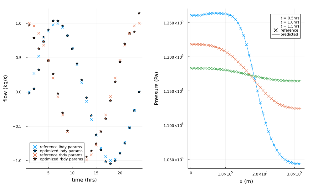
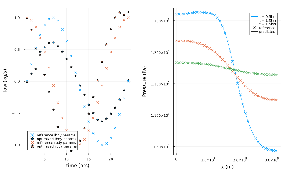
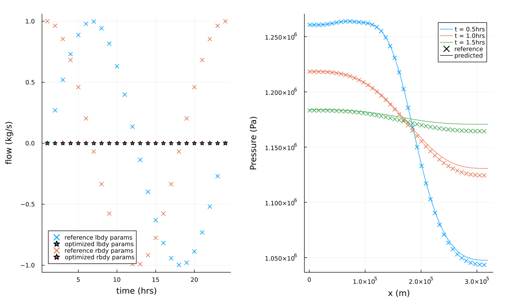
Figure 4: Results for the optimization in Eq. (10) for a pipe of 200mi over a 24hr forecast. The panels show (top) $\alpha=0$, (middle) $\alpha=0.5$, and (bottom) $\alpha=1$. The left plots show the reference and optimized boundary conditions, while the right plots show the first hours of the pressure evolution along the pipe. The initial condition is a constant pressure of 10bar, with a Gaussian bump at $x=100m$.

We also use this simple example to benchmark the method for compuation complexity. As shown in Fig. (5) we achieve computation complexity of $\mathcal{O}(N_{x}\cdot N_{t})$ for the forward and gradient calculations, with $N_{x}$ the number of spatial discretization points and $N_{t}$ the number of timesteps. Of particular note is the absence of sensitivity of computation time to the number of parameters $N_{p}$ - this suggests desirable scaling when extending this method to more complex parameterizations.

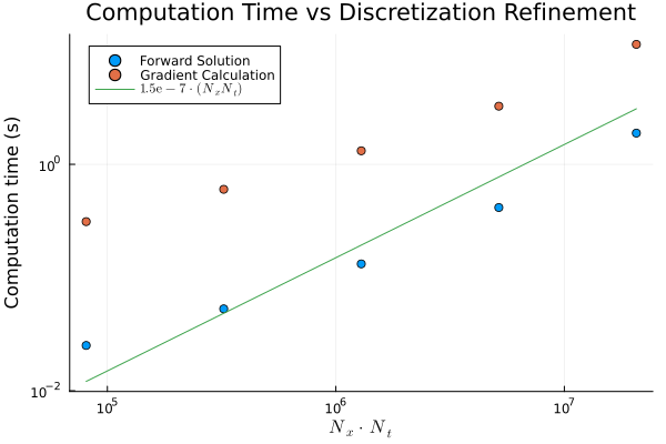
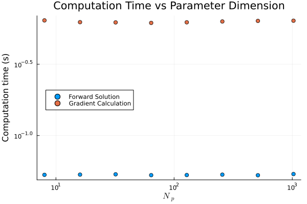
Figure 5:

3.2 Small Network

We now apply the method to optimize the meaningful objective Eq. (9) on a 4 pipe network shown in Fig. (6). We use the artificial demand curve

$$D(t)=200\cdot\sin\left(2\pi\frac{t}{T}\right)+400$$ (11)

with linear gas withdrawal cost, $E(\psi)=\max(0,\psi)$, where $\psi$ is positive if gas is being withdrawn from the network, and negative if gas is being injected into the network.

Our network has one supply node (node 1), and three power plants (PP1, PP2, PP3), at nodes 2, 3, and 4, respectively. PP1 and PP3 are about 30% more efficient than PP2, and we thus expect the network to use their capacity first.

The results of the optimization are shown in Fig. 6, where the top panel shows the energy demand and production, as well as contributions from the individual power plants. The bottom two panels show the pressures throughout the network at start and end, (animations showing the full temporal evolution of the pressure are available online https://github.com/cmhyett/DiffGasNetworks).

In practice, we want first and foremost to ensure the network does not violate pressure constraints (minimum pressure crossings can lead to loss of generators and thus outages), second to ensure generated power meets demand, and third to provide power at the lowest cost. This leads to the ordering of hyperparameters $\gamma\gg\alpha>\beta$ in Eq. (9). During our optimization, pressure falls, and PP3 being at the end of the network is most vulnerable to a low pressure crossing - thus PP2, despite having a higher generation cost supplements the generation during hours 5 and 6.

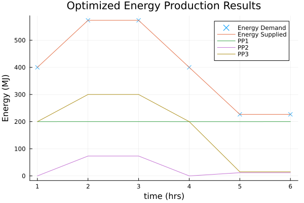
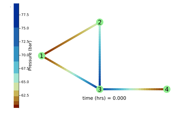
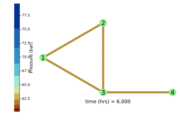
Figure 6: Results for the optimization in Eq. (10) for a network of 4 pipes, each 70km long, and with varying widths and friction factors. Power plants 1 and 3 are about $30\%$ more efficient than power plant 2. At late times, the optimization prefers the higher cost of running plant 2 to incurring a pressure penalty at plant 3 (node 4).

4 Conclusion & Path Forward

The primary technical advancement of this manuscript lies in the harmonization of three distinct components for resolving the stochastic optimal gas flow problem – where stochasticity is incorporated via samples while seeking the stationary point of the respective augmented Lagrangian:

1. Efficient Gas-Flow Implementation: Our approach leverages the explicit staggered-grid method for forward-in-time primal equations, streamlining the computational treatment of the gas flows.

2. Integration with SciML/Julia Ecosystem: By integrating our forward framework into the SciML/Julia ecosystem, we seamlessly gain access to automatic sensitivity analysis. This, in turn, facilitates the handling of adjoint (backward-in-time) equations automatically.

3. Simple Gas-Power Coupling: The inter-dependency between gas and power is accounted for through nodal flows, providing a straightforward formalization of the two energy infrastructure inter-dependency.

We demonstrated the method achieved optimal computation scaling in both the forward and gradient calculations. The method was applied to solve optimizations on a single pipe system and subsequently on a more intricate four-node system, each containing nontrivial transient dynamics.

Should our manuscript be accepted for PSCC, we plan to augment the final version with additional experimental data. Specifically, we aim to test our proposed methodology on a realistic 11-node representation of Israel’s gas system.

Looking ahead, our future objectives encompass:

• Enhanced Power Systems Modeling: We plan to bolster our already sufficiently exhaustive gas-grid network model by integrating a more comprehensive representation of power systems. This enhancement will address aspects like power losses and will allow to extend optimization to other resources on the power system side beyond just the gas-power plants.

• Accounting for Emergencies: We plan to integrate this research with a related study, which our team has also submitted to PSCC. This partner study delves deeper into emergency scenarios, particularly focusing on more challenging operational conditions.

• Long-Term Adaptations for Israel’s Gas-Grid System: Our ultimate ambition is to tailor this framework not only for operations but also for operations-aware planning of Israel’s gas-grid system. Among other facets, this will involve the evaluation and comparison of potential extensions, like the inclusion of gas storage, compressors, batteries and evaluation various energy export options.

Appendices

4.1 Adjoint Method

In order to utilize gradient descent algorithms to optimize Eq (8), we must compute $d_{q}O(u,q)$ with

$$O(u,q)=\int_{0}^{T}C(u,q,t)\,dt$$ (12)

and $C:=\text{Cost}$. By construction, we have that $g(u,\dot{u},q,t)=0$ specifying the differential equation, and $h(u(0),q)=0$ specifying the initial condition. Thus, we can rephrase this optimization using the Lagrangian formulation

$$\mathcal{L}:=\int_{0}^{T}\left[C(u,q,t)+\lambda^{T}g(u,\dot{u},q,t)\right]dt+\mu^{T}h(u(0),q),$$ (13)

where $\lambda$ and $\mu$ are the Lagrangian multipliers associated with the dynamics and initial condition, respectively. Notice that $d_{q}O=d_{q}{\cal L}$ since $g(u,\dot{u},q,t)=h(u(0),q)=0$ everywhere by construction. This equality additionally gives us complete freedom to choose $\lambda,\mu$ (with $\lambda$ dependent on time).

Then we compute

$$d_{q}{\cal L}=\int_{0}^{T}(\partial_{u}Cd_{q}u+\partial_{q}C)\\ +\lambda^{T}\left(\partial_{u}gd_{q}u+\partial_{\dot{u}}gd_{q}\dot{u}+\partial_{q}g\right)dt\\ +\mu^{T}\left(\partial_{u(0)}hd_{q}u(0)+\partial_{q}h\right)$$ (14)

We can use integration by parts to express $d_{q}\dot{u}$ in terms of $d_{q}u$

$$\int_{0}^{T}\lambda^{T}\partial_{\dot{u}}gd_{q}\dot{u}\,dt=\\ \left[\lambda^{T}\partial_{\dot{u}}gd_{q}u\right|_{0}^{T}-\int_{0}^{T}\left(\lambda^{T}d_{t}\partial_{\dot{u}}g+\dot{\lambda}^{T}\partial_{\dot{u}}g\right)d_{q}u\,dt$$ (15)

Substituting Eq (15) into Eq (14) and collecting terms in $d_{q}u$ and $d_{q}u(0)$

$$d_{q}\mathcal{L}=\\ \int_{0}^{T}\Big{[}\left(\partial_{u}C\mkern-5.0mu+\mkern-5.0mu\lambda^{T}\mkern-7.0mu\left(\partial_{u}g\mkern-5.0mu-\mkern-5.0mud_{t}\partial_{\dot{u}}g\right)\mkern-5.0mu-\mkern-5.0mu\dot{\lambda}^{T}\partial_{\dot{u}}g\right)d_{q}u+\partial_{q}C+\lambda^{T}\partial_{q}g\Big{]}dt\\ +\left[\lambda^{T}\partial_{\dot{u}}gd_{q}u\right|_{T}+\left[\mu^{T}\partial_{u}h-\lambda^{T}\partial_{\dot{u}}g\right|_{0}d_{q}u(0)+\mu^{T}d_{q}h.$$ (16)

We now begin exploiting freedom in $\lambda,\mu$ to avoid calculation of $d_{q}u$. Set

$$\lambda(T)=0\ \implies\left[\lambda^{T}\partial_{\dot{u}}gd_{q}u\right|_{T}=0$$ (17)

$$\mu^{T}=\left[\lambda^{T}\partial_{\dot{u}}g\right|_{0}\left(\partial_{u(0)}g\right)^{-1} \implies\left[\mu^{T}\partial_{u(0)}h-\lambda^{T}\partial_{\dot{u}}g\right|_{0}=0$$ (18)

Then we have

$$d_{q}\mathcal{L}=\int_{0}^{T}\Big{[}\left(d_{q}C+\lambda^{T}\left(\partial_{u}g-d_{t}\partial_{\dot{u}}g\right)+\dot{\lambda}^{T}\partial_{\dot{u}}g\right)d_{q}u\\ +\lambda^{T}\partial_{q}g\Big{]}dt\\ +\left[\lambda^{T}\partial_{\dot{u}}g\right|_{0}\left(\partial_{u(0)}h\right)^{-1}d_{q}h$$ (19)

We still have freedom to set $\lambda(t)$ for $t\in[0,T)$. Thus, once again to avoid $d_{q}u$, solve for $\lambda$ backward in time from

$$\begin{split}\partial_{q}C+\lambda^{T}\left(\partial_{u}g-d_{t}\partial_{\dot{u}}g\right)+\dot{\lambda}^{T}\partial_{\dot{u}}g=0\\ \text{with }\lambda(T)=0\end{split}$$ (20)

We then have

$$\begin{split}d_{q}\mathcal{L}&=d_{q}O=\\ &\int_{0}^{T}\big{(}d_{q}C+\lambda^{T}\partial_{q}g\big{)}\,dt+\left[\dot{\lambda}^{T}\partial_{\dot{u}}g\right|_{0}\left(\partial_{u(0)}h\right)^{-1}d_{q}h\end{split}$$ (21)

Thus, solving Eq. (20) allows performing the integration Eq. (21), at which time we have the desired gradient $d_{q}O$ and can take an optimization step.

Notice that we still have a functional forms to determine, and these functions depend on the solved state $u$, e.g., $d_{q}C(u,q,t),\partial_{u}g(u,\dot{u},q,t)$, etc. We use source-to-source AD to determine and evaluate these functional forms.

4.2 Differentiable Programming

Source-to-source differentiation, particularly from Zygote.jl [12], is a transformational capability that allows reverse-mode automatic differentiation (AD) through programming language constructs – enabling optimized adjoint function evaluation without the need to write the derivatives by hand. This freedom ensures correctness, and allows for generality in construction of the forward pass [13].

In order to compute the integral Eq. (21), the adjoint ODE Eq. (20) is solved for $\lambda(t)$, and the term $\partial_{q}g$ is found via source-to-source reverse-mode AD. This method to compute the adjoint has computational cost that scales linearly with the forward pass, and with the number of parameters [14]. Thus, while other methods of gradient calculation are more efficient for small numbers of parameters, we choose the adjoint using AD in anticipation of extension of the optimization problem to large networks with varying configurations.

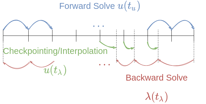
Figure 7: Schematic of adjoint method implementation, where the adjoint ODE utilizes checkpointing to accelerate queries of the state $u$ at required times.[14]

References

- [1] A. Zlotnik, L. Roald, S. Backhaus, M. Chertkov, and G. Andersson, “Coordinated scheduling for interdependent electric power and natural gas infrastructures,” IEEE Transactions on Power Systems, vol. 32, no. 1, pp. 600–610, 2016.
- [2] G. Byeon and P. Van Hentenryck, “Unit commitment with gas network awareness,” IEEE Transactions on Power Systems, vol. 35, no. 2, pp. 1327–1339, 2019.
- [3] L. S. Baker, S. Shivakumar, D. Armbruster, R. B. Platte, and A. Zlotnik, “Linear system analysis and optimal control of natural gas dynamics in pipeline networks,” 2023.
- [4] M. Innes, A. Edelman, K. Fischer, C. Rackauckas, E. Saba, V. B. Shah, and W. Tebbutt, “A differentiable programming system to bridge machine learning and scientific computing,” arXiv preprint arXiv:1907.07587, 2019.
- [5] V. Gyrya and A. Zlotnik, “An explicit staggered-grid method for numerical simulation of large-scale natural gas pipeline networks,” Applied Mathematical Modelling, vol. 65, pp. 34–51, 2019.
- [6] C. Rackauckas, Y. Ma, J. Martensen, C. Warner, K. Zubov, R. Supekar, D. Skinner, and A. Ramadhan, “Universal differential equations for scientific machine learning,” arXiv preprint arXiv:2001.04385, 2020.
- [7] C. Hyett, L. Pagnier, J. Alisse, L. Sabban, I. Goldshtein, and M. Chertkov, “Control of line pack in natural gas system: Balancing limited resources under uncertainty,” in PSIG Annual Meeting. PSIG, 2023, pp. PSIG–2314.
- [8] A. Osiadacz, “Simulation of transient gas flows in networks,” International Journal for Numerical Methods in Fluids, vol. 4, no. 1, pp. 13–24, Jan. 1984. [Online]. Available: https://onlinelibrary.wiley.com/doi/10.1002/fld.1650040103
- [9] M. C. Steinbach, “On PDE solution in transient optimization of gas networks,” Journal of Computational and Applied Mathematics, vol. 203, no. 2, pp. 345–361, Jun. 2007. [Online]. Available: https://linkinghub.elsevier.com/retrieve/pii/S0377042706002263
- [10] E. S. Menon, Gas Pipeline Hydraulics. CRC Press, 2005.
- [11] M. Brio, G. M. Webb, and A. R. Zakharian, Numerical time-dependent partial differential equations for scientists and engineers. Academic Press, 2010.
- [12] M. Innes, “Don’t unroll adjoint: Differentiating ssa-form programs,” 2019.
- [13] C. Rackauckas, Sciemon, J. Vaverka, B. S. Zhu, V. L., A. Strouwen, D. P. Sanders, G. Sterpu, J. Ling, P. E. Catach, P. Monticone, W. Dey, V. Churavy, A. Edelman, A. Haslam, A. Lenail, A. Kaushal, C. Laforte, C. Wang, F. Cucchietti, K. Bhogaonker, L. Milechin, F. C. White, M. Payne, S. Schaub, S. Fu, V. Meijer, W. Kirchgässner, and anand jain, “Sciml/scimlbook: v1.1,” Nov. 2022. [Online]. Available: https://doi.org/10.5281/zenodo.7347643
- [14] Y. Ma, V. Dixit, M. J. Innes, X. Guo, and C. Rackauckas, “A comparison of automatic differentiation and continuous sensitivity analysis for derivatives of differential equation solutions,” in 2021 IEEE High Performance Extreme Computing Conference (HPEC), 2021, pp. 1–9.