Variance-based sensitivity of Bayesian inverse problems to the prior distribution

Abstract

The formulation of Bayesian inverse problems involves choosing prior distributions; choices that seem equally reasonable may lead to significantly different conclusions. We develop a computational approach to better understand the impact of the hyperparameters defining the prior on the posterior statistics of the quantities of interest. Our approach relies on global sensitivity analysis (GSA) of Bayesian inverse problems with respect to the hyperparameters defining the prior. This, however, is a challenging problem—a naive double loop sampling approach would require running a prohibitive number of Markov chain Monte Carlo (MCMC) sampling procedures. The present work takes a foundational step in making such a sensitivity analysis practical through (i) a judicious combination of efficient surrogate models and (ii) a tailored importance sampling method. In particular, we can perform accurate GSA of posterior prediction statistics with respect to prior hyperparameters without having to repeat MCMC runs. We demonstrate the effectiveness of the approach on a simple Bayesian linear inverse problem and a nonlinear inverse problem governed by an epidemiological model.

[label1]organization=Department of Mathematics, North Carolina State University, city=Raleigh, state=NC, country=USA [label2]organization=The Graduate School, North Carolina State University, city=Raleigh, state=NC, country=USA

1 Introduction

Consider a Bayesian inverse problem governed by a system of differential equations. The inverse problem uses a vector $\textstyle{d}$ of measurement data to estimate the uncertain model parameters, $\textstyle{\theta}$. The solution of the Bayesian inverse problem is a posterior distribution $\pi_{\mathrm{post}}({\mathchoice{\mbox{\boldmath$\displaystyle{\theta}$}}{\mbox{\boldmath$\textstyle{\theta}$}}{\mbox{\boldmath$\scriptstyle{\theta}$}}{\mbox{\boldmath$\scriptscriptstyle{\theta}$}}}|{\mathchoice{\mbox{\boldmath$\displaystyle{d}$}}{\mbox{\boldmath$\textstyle{d}$}}{\mbox{\boldmath$\scriptstyle{d}$}}{\mbox{\boldmath$\scriptscriptstyle{d}$}}})$. After solving the inverse problem, typically we seek to make some predictions based on the posterior. For example, for a prediction quantity $q({\mathchoice{\mbox{\boldmath$\displaystyle{\theta}$}}{\mbox{\boldmath$\textstyle{\theta}$}}{\mbox{\boldmath$\scriptstyle{\theta}$}}{\mbox{\boldmath$\scriptscriptstyle{\theta}$}}})$ we may consider

$$\mathbb{E}_{\mathrm{post}}(q):=\int q({\mathchoice{\mbox{\boldmath$\displaystyle{\theta}$}}{\mbox{\boldmath$\textstyle{\theta}$}}{\mbox{\boldmath$\scriptstyle{\theta}$}}{\mbox{\boldmath$\scriptscriptstyle{\theta}$}}})\pi_{\mathrm{post}}({\mathchoice{\mbox{\boldmath$\displaystyle{\theta}$}}{\mbox{\boldmath$\textstyle{\theta}$}}{\mbox{\boldmath$\scriptstyle{\theta}$}}{\mbox{\boldmath$\scriptscriptstyle{\theta}$}}}|{\mathchoice{\mbox{\boldmath$\displaystyle{d}$}}{\mbox{\boldmath$\textstyle{d}$}}{\mbox{\boldmath$\scriptstyle{d}$}}{\mbox{\boldmath$\scriptscriptstyle{d}$}}})\,d{\mathchoice{\mbox{\boldmath$\displaystyle{\theta}$}}{\mbox{\boldmath$\textstyle{\theta}$}}{\mbox{\boldmath$\scriptstyle{\theta}$}}{\mbox{\boldmath$\scriptscriptstyle{\theta}$}}}.$$

A crucial component of this analysis is to know how the choice of prior hyperparameters affects such predictions. We present a practical variance-based global sensitivity analysis (GSA) approach to study how statistics (e.g. mean or variance) of $q$ vary with respect to prior hyperparameters. This enables us to identify which prior hyperparameters carry the most influence over the prediction.

Bayesian inference is pervasive; this perspective makes inferences not just from data, but also by incorporating prior beliefs and assumptions. In practice, these prior assumptions are often subjective choices made by the researcher. However, these prior beliefs can have a huge impact on the results, including those of Bayesian inverse problems [1]. This well-known issue motivated statisticians in the 1980s and 1990s to develop a methodology, known as robust Bayesian analysis [2, 3, 4, 5], for ensuring the robustness of Bayesian inference to different choices by the researcher. These ideas have continued to receive attention over the past two decades [6, 7, 8, 9, 10, 11].

Related work. Sensitivity analysis of Bayesian inverse problems has been subject to several recent research efforts. The articles [12, 13, 14] consider hyper-differential sensitivity analysis (HDSA) of Bayesian inverse problems. HDSA is a technique used originally for (deterministic) PDE-constrained optimization problems. HDSA, as a practical framework for sensitivity analysis of optimal control problems governed by PDEs, was considered in [15]. In [16], HDSA was used for sensitivity analysis of deterministic inverse problems to auxiliary model parameters and parameters specifying the experimental setup (experimental parameters). In [12], use of HDSA is extended to nonlinear Bayesian inverse problems. Specifically, the authors consider the Bayes risk and the maximum a posterior probability (MAP) point as quantities of interest for sensitivity analysis. In [13], the HDSA framework is used to study Bayesian inverse problems governed by ice sheet models. The sensitivity of information gain, measured by the Kullback–Leibler (KL) divergence between the prior and posterior, to uncertain model parameters in linear Bayesian inverse problems is studied in [14]. HDSA provides valuable insight for experimenters on where to focus resources during experimental design and when measuring auxiliary parameters. The previous works on HDSA of Bayesian inverse problems, have focused primarily on sensitivity analysis with respect to auxiliary or experimental rather than prior hyperparameters. More importantly, HDSA is local, relying on derivative information evaluated at a set of nominal parameters. Variance-based GSA, see Section 3, accounts for the uncertainty in the hyperparameters globally.

The work [17], which is closely related to our work, examines single-parameter statistical models using Bayesian inference. In that paper, the authors perform variance-based GSA on posterior statistics with respect to prior and auxiliary hyperparameters. Their method uses Gaussian process (GP) surrogates to emulate the mapping from the hyperparameters to the posterior distribution. This method requires many Markov chain Monte Carlo (MCMC) runs to build the GP surrogate. For the Bayesian inverse problems we target, the high cost of evaluating the forward model makes repeated MCMC runs impossible. We tackle this difficulty by using an importance sampling approach that allows integrating the QoIs under study with respect to multiple posterior distributions. Strategies for importance sampling on multiple distributions have been subject to several previous works; see e.g., [18, 19, 20, 21, 22]. We use the structure of the Bayesian inverse problem to derive a tailored importance sampling approach. Another related work that has partly inspired the approach in the present work is [23]. That article, outlines a method for GSA of rare event probabilities that combines surrogate-assisted GSA with subset simulation.

Our approach and contributions. We show that GSA is a viable computational approach to analyze the sensitivity of Bayesian inverse problems to prior hyperparameters. The proposed approach is goal oriented—the focus is on the posterior statistics of prediction/goal QoIs that are functions of the inversion parameters. We first frame the problem in a manner conducive to variance-based GSA in Section 2. We detail the computational strategy for sensitivity analysis in Section 4. Our method combines two key techniques. Importance sampling eliminates the need for repeated MCMC runs for different choices of the prior. Then, sparse polynomial chaos expansion (PCE) and extreme learning machine (ELM) surrogate models emulate the mapping from prior hyperparameters to statistics of $q$. Use of surrogate models not only eases the computational burden, but also improves the accuracy of the sensitivity analysis. The combined approach enables prior hyperparameter sensitivity analysis for many Bayesian inverse problems. If one has access to a single MCMC run, then one can ascertain prior hyperparameter importance. To demonstrate the effectiveness of the proposed approach, we present extensive computational experiments in the context of two examples: a simple linear inverse problem in Section 5.1 and a nonlinear inverse problem governed by an epidemiological model in Section 5.2.

2 Hyperparameter-to-statistic mapping of Bayesian inverse problems

In an inverse problem [24], we use a model and observed data to estimate unknown model parameters of interest. We consider the inverse problem of estimating a parameter vector $\textstyle{\theta}$ in models of the form

$$\left\{\begin{aligned} &{\mathchoice{\mbox{\boldmath$\displaystyle{y}$}}{\mbox{\boldmath$\textstyle{y}$}}{\mbox{\boldmath$\scriptstyle{y}$}}{\mbox{\boldmath$\scriptscriptstyle{y}$}}}^{\prime}=f({\mathchoice{\mbox{\boldmath$\displaystyle{y}$}}{\mbox{\boldmath$\textstyle{y}$}}{\mbox{\boldmath$\scriptstyle{y}$}}{\mbox{\boldmath$\scriptscriptstyle{y}$}}};{\mathchoice{\mbox{\boldmath$\displaystyle{\theta}$}}{\mbox{\boldmath$\textstyle{\theta}$}}{\mbox{\boldmath$\scriptstyle{\theta}$}}{\mbox{\boldmath$\scriptscriptstyle{\theta}$}}}),\\ &{\mathchoice{\mbox{\boldmath$\displaystyle{y}$}}{\mbox{\boldmath$\textstyle{y}$}}{\mbox{\boldmath$\scriptstyle{y}$}}{\mbox{\boldmath$\scriptscriptstyle{y}$}}}(t_{0})={\mathchoice{\mbox{\boldmath$\displaystyle{y}$}}{\mbox{\boldmath$\textstyle{y}$}}{\mbox{\boldmath$\scriptstyle{y}$}}{\mbox{\boldmath$\scriptscriptstyle{y}$}}}_{0}.\end{aligned}\right.$$ (1)

Here, ${\mathchoice{\mbox{\boldmath$\displaystyle{y}$}}{\mbox{\boldmath$\textstyle{y}$}}{\mbox{\boldmath$\scriptstyle{y}$}}{\mbox{\boldmath$\scriptscriptstyle{y}$}}}\in\mathbb{R}^{d}$ is the state vector. In a deterministic formulation of the inverse problem, we typically seek a $\textstyle{\theta}$ that minimizes the cost functional,

$$J({\mathchoice{\mbox{\boldmath$\displaystyle{\theta}$}}{\mbox{\boldmath$\textstyle{\theta}$}}{\mbox{\boldmath$\scriptstyle{\theta}$}}{\mbox{\boldmath$\scriptscriptstyle{\theta}$}}}):=\|\mathbf{{B}}{\mathchoice{\mbox{\boldmath$\displaystyle{y}$}}{\mbox{\boldmath$\textstyle{y}$}}{\mbox{\boldmath$\scriptstyle{y}$}}{\mbox{\boldmath$\scriptscriptstyle{y}$}}}({\mathchoice{\mbox{\boldmath$\displaystyle{\theta}$}}{\mbox{\boldmath$\textstyle{\theta}$}}{\mbox{\boldmath$\scriptstyle{\theta}$}}{\mbox{\boldmath$\scriptscriptstyle{\theta}$}}})-{\mathchoice{\mbox{\boldmath$\displaystyle{d}$}}{\mbox{\boldmath$\textstyle{d}$}}{\mbox{\boldmath$\scriptstyle{d}$}}{\mbox{\boldmath$\scriptscriptstyle{d}$}}}\|^{2}.$$ (2)

Here, $\textstyle{d}$ is a vector of data measurements, $\mathbf{{B}}$ is a linear operator that selects the corresponding model responses, and $\textstyle{y}$ is obtained by solving (1).

We focus on Bayesian inverse problems [24] and seek a statistical distribution for $\textstyle{\theta}$, known as the posterior distribution, that is conditioned on the observed data and is consistent with the prior distribution. In this context, the prior distribution encodes our prior knowledge regarding the parameters. The Bayes formula shows how the model, data, and the prior are combined to obtain the posterior distribution:

$$\pi_{\mathrm{post}}({\mathchoice{\mbox{\boldmath$\displaystyle{\theta}$}}{\mbox{\boldmath$\textstyle{\theta}$}}{\mbox{\boldmath$\scriptstyle{\theta}$}}{\mbox{\boldmath$\scriptscriptstyle{\theta}$}}}|{\mathchoice{\mbox{\boldmath$\displaystyle{d}$}}{\mbox{\boldmath$\textstyle{d}$}}{\mbox{\boldmath$\scriptstyle{d}$}}{\mbox{\boldmath$\scriptscriptstyle{d}$}}})\propto\pi_{\mathrm{like}}({\mathchoice{\mbox{\boldmath$\displaystyle{d}$}}{\mbox{\boldmath$\textstyle{d}$}}{\mbox{\boldmath$\scriptstyle{d}$}}{\mbox{\boldmath$\scriptscriptstyle{d}$}}}|{\mathchoice{\mbox{\boldmath$\displaystyle{\theta}$}}{\mbox{\boldmath$\textstyle{\theta}$}}{\mbox{\boldmath$\scriptstyle{\theta}$}}{\mbox{\boldmath$\scriptscriptstyle{\theta}$}}})\times\pi_{\mathrm{pr}}({\mathchoice{\mbox{\boldmath$\displaystyle{\theta}$}}{\mbox{\boldmath$\textstyle{\theta}$}}{\mbox{\boldmath$\scriptstyle{\theta}$}}{\mbox{\boldmath$\scriptscriptstyle{\theta}$}}}),$$ (3)

where $\pi_{\mathrm{like}}$ is the data likelihood and $\pi_{\mathrm{pr}}$ is the prior probability density function (PDF). Throughout this paper, we assume a Gaussian noise model for the observation error. In this case, the Bayes formula reads

$$\pi_{\mathrm{post}}({\mathchoice{\mbox{\boldmath$\displaystyle{\theta}$}}{\mbox{\boldmath$\textstyle{\theta}$}}{\mbox{\boldmath$\scriptstyle{\theta}$}}{\mbox{\boldmath$\scriptscriptstyle{\theta}$}}}|{\mathchoice{\mbox{\boldmath$\displaystyle{d}$}}{\mbox{\boldmath$\textstyle{d}$}}{\mbox{\boldmath$\scriptstyle{d}$}}{\mbox{\boldmath$\scriptscriptstyle{d}$}}})\propto\text{exp}\big{(}{-\frac{1}{2}(\textbf{B}{\mathchoice{\mbox{\boldmath$\displaystyle{y}$}}{\mbox{\boldmath$\textstyle{y}$}}{\mbox{\boldmath$\scriptstyle{y}$}}{\mbox{\boldmath$\scriptscriptstyle{y}$}}}({\mathchoice{\mbox{\boldmath$\displaystyle{\theta}$}}{\mbox{\boldmath$\textstyle{\theta}$}}{\mbox{\boldmath$\scriptstyle{\theta}$}}{\mbox{\boldmath$\scriptscriptstyle{\theta}$}}})-{\mathchoice{\mbox{\boldmath$\displaystyle{d}$}}{\mbox{\boldmath$\textstyle{d}$}}{\mbox{\boldmath$\scriptstyle{d}$}}{\mbox{\boldmath$\scriptscriptstyle{d}$}}})^{\top}\Gamma_{\mathrm{noise}}^{-1}(\textbf{B}{\mathchoice{\mbox{\boldmath$\displaystyle{y}$}}{\mbox{\boldmath$\textstyle{y}$}}{\mbox{\boldmath$\scriptstyle{y}$}}{\mbox{\boldmath$\scriptscriptstyle{y}$}}}({\mathchoice{\mbox{\boldmath$\displaystyle{\theta}$}}{\mbox{\boldmath$\textstyle{\theta}$}}{\mbox{\boldmath$\scriptstyle{\theta}$}}{\mbox{\boldmath$\scriptscriptstyle{\theta}$}}})-{\mathchoice{\mbox{\boldmath$\displaystyle{d}$}}{\mbox{\boldmath$\textstyle{d}$}}{\mbox{\boldmath$\scriptstyle{d}$}}{\mbox{\boldmath$\scriptscriptstyle{d}$}}})}\big{)}\times\pi_{\mathrm{pr}}({\mathchoice{\mbox{\boldmath$\displaystyle{\theta}$}}{\mbox{\boldmath$\textstyle{\theta}$}}{\mbox{\boldmath$\scriptstyle{\theta}$}}{\mbox{\boldmath$\scriptscriptstyle{\theta}$}}}),$$ (4)

where $\Gamma_{\mathrm{noise}}^{-1}$ is the noise covariance.

In practice, we are often interested in scalar prediction quantities of interest (QoIs) that depend on $\textstyle{\theta}$. Let $q({\mathchoice{\mbox{\boldmath$\displaystyle{\theta}$}}{\mbox{\boldmath$\textstyle{\theta}$}}{\mbox{\boldmath$\scriptstyle{\theta}$}}{\mbox{\boldmath$\scriptscriptstyle{\theta}$}}})$ be such a QoI. Solving the Bayesian inverse problem enables reducing the uncertainty in $\textstyle{\theta}$ and consequently in $q({\mathchoice{\mbox{\boldmath$\displaystyle{\theta}$}}{\mbox{\boldmath$\textstyle{\theta}$}}{\mbox{\boldmath$\scriptstyle{\theta}$}}{\mbox{\boldmath$\scriptscriptstyle{\theta}$}}})$. In this case, the statistical properties of $q$ depend on $\pi_{\mathrm{post}}$. Let $\Psi(q)$ denote a generic statistic of $q$. Examples include $\Psi(q)=\mathrm{var}(q)$ or $\Psi(q)=\mathbb{E}(q)$, where the expectation and variance are with respect to the posterior distribution. Another example is $\Psi(q)=q({\mathchoice{\mbox{\boldmath$\displaystyle{\theta}$}}{\mbox{\boldmath$\textstyle{\theta}$}}{\mbox{\boldmath$\scriptstyle{\theta}$}}{\mbox{\boldmath$\scriptscriptstyle{\theta}$}}}_{\mathrm{MAP}})$; i.e, QoI evaluated at the maximum a posteriori (MAP) point estimate of $\textstyle{\theta}$. Recall that the MAP point, ${\mathchoice{\mbox{\boldmath$\displaystyle{\theta}$}}{\mbox{\boldmath$\textstyle{\theta}$}}{\mbox{\boldmath$\scriptstyle{\theta}$}}{\mbox{\boldmath$\scriptscriptstyle{\theta}$}}}_{\mathrm{MAP}}$, is a point where the posterior PDF attains its maximum value. Using the Bayes formula (4), we note that the MAP point is the solution to the nonlinear least squares problem

$${\mathchoice{\mbox{\boldmath$\displaystyle{\theta}$}}{\mbox{\boldmath$\textstyle{\theta}$}}{\mbox{\boldmath$\scriptstyle{\theta}$}}{\mbox{\boldmath$\scriptscriptstyle{\theta}$}}}_{\mathrm{MAP}}=\underset{{\mathchoice{\mbox{\boldmath$\displaystyle{\theta}$}}{\mbox{\boldmath$\textstyle{\theta}$}}{\mbox{\boldmath$\scriptstyle{\theta}$}}{\mbox{\boldmath$\scriptscriptstyle{\theta}$}}}}{\mathrm{argmin}}\;J({\mathchoice{\mbox{\boldmath$\displaystyle{\theta}$}}{\mbox{\boldmath$\textstyle{\theta}$}}{\mbox{\boldmath$\scriptstyle{\theta}$}}{\mbox{\boldmath$\scriptscriptstyle{\theta}$}}})\vcentcolon=(\textbf{B}{\mathchoice{\mbox{\boldmath$\displaystyle{y}$}}{\mbox{\boldmath$\textstyle{y}$}}{\mbox{\boldmath$\scriptstyle{y}$}}{\mbox{\boldmath$\scriptscriptstyle{y}$}}}({\mathchoice{\mbox{\boldmath$\displaystyle{\theta}$}}{\mbox{\boldmath$\textstyle{\theta}$}}{\mbox{\boldmath$\scriptstyle{\theta}$}}{\mbox{\boldmath$\scriptscriptstyle{\theta}$}}})-{\mathchoice{\mbox{\boldmath$\displaystyle{d}$}}{\mbox{\boldmath$\textstyle{d}$}}{\mbox{\boldmath$\scriptstyle{d}$}}{\mbox{\boldmath$\scriptscriptstyle{d}$}}})^{\top}\Gamma_{\mathrm{noise}}^{-1}(\textbf{B}{\mathchoice{\mbox{\boldmath$\displaystyle{y}$}}{\mbox{\boldmath$\textstyle{y}$}}{\mbox{\boldmath$\scriptstyle{y}$}}{\mbox{\boldmath$\scriptscriptstyle{y}$}}}({\mathchoice{\mbox{\boldmath$\displaystyle{\theta}$}}{\mbox{\boldmath$\textstyle{\theta}$}}{\mbox{\boldmath$\scriptstyle{\theta}$}}{\mbox{\boldmath$\scriptscriptstyle{\theta}$}}})-{\mathchoice{\mbox{\boldmath$\displaystyle{d}$}}{\mbox{\boldmath$\textstyle{d}$}}{\mbox{\boldmath$\scriptstyle{d}$}}{\mbox{\boldmath$\scriptscriptstyle{d}$}}})-2\log(\pi_{\mathrm{pr}}({\mathchoice{\mbox{\boldmath$\displaystyle{\theta}$}}{\mbox{\boldmath$\textstyle{\theta}$}}{\mbox{\boldmath$\scriptstyle{\theta}$}}{\mbox{\boldmath$\scriptscriptstyle{\theta}$}}})).$$ (5)

We consider how the choice of prior affects $\Psi(q)$. Narrowing this question, we take a parameterized family of prior distributions $\pi_{\mathrm{pr}}^{{\mathchoice{\mbox{\boldmath$\displaystyle{\xi}$}}{\mbox{\boldmath$\textstyle{\xi}$}}{\mbox{\boldmath$\scriptstyle{\xi}$}}{\mbox{\boldmath$\scriptscriptstyle{\xi}$}}}}({\mathchoice{\mbox{\boldmath$\displaystyle{\theta}$}}{\mbox{\boldmath$\textstyle{\theta}$}}{\mbox{\boldmath$\scriptstyle{\theta}$}}{\mbox{\boldmath$\scriptscriptstyle{\theta}$}}})$ determined by a vector $\textstyle{\xi}$ of scalar hyperparameters. For a Gaussian prior, the hyperparameters can be taken as the prior means and variances. With this setup, the choice of $\textstyle{\xi}$ will determine our statistic of interest so that $\Psi(q)=\Psi^{{\mathchoice{\mbox{\boldmath$\displaystyle{\xi}$}}{\mbox{\boldmath$\textstyle{\xi}$}}{\mbox{\boldmath$\scriptstyle{\xi}$}}{\mbox{\boldmath$\scriptscriptstyle{\xi}$}}}}(q)$. In what follows, the hyperparameter-to-statistic (HS) mapping $F:\mathbb{R}^{n}\to\mathbb{R}$ is given by

$$F({\mathchoice{\mbox{\boldmath$\displaystyle{\xi}$}}{\mbox{\boldmath$\textstyle{\xi}$}}{\mbox{\boldmath$\scriptstyle{\xi}$}}{\mbox{\boldmath$\scriptscriptstyle{\xi}$}}})\vcentcolon=\Psi^{{\mathchoice{\mbox{\boldmath$\displaystyle{\xi}$}}{\mbox{\boldmath$\textstyle{\xi}$}}{\mbox{\boldmath$\scriptstyle{\xi}$}}{\mbox{\boldmath$\scriptscriptstyle{\xi}$}}}}(q).$$ (6)

To model the uncertainty in the hyperparameters, we consider them as random variables and then analyze how the uncertainty in the entries of $\textstyle{\xi}$ contributes to the uncertainty in $F({\mathchoice{\mbox{\boldmath$\displaystyle{\xi}$}}{\mbox{\boldmath$\textstyle{\xi}$}}{\mbox{\boldmath$\scriptstyle{\xi}$}}{\mbox{\boldmath$\scriptscriptstyle{\xi}$}}})$. To this end, we follow a variance-based sensitivity analysis framework, and compute the Sobol’ indices [25, 26] of the HS mapping $F$ with respect to $\textstyle{\xi}$.

For the purposes of this study, we let the prior hyperparameters $\textstyle{\xi}$ follow uniform distributions, $\xi_{j}\sim\mathcal{U}[a_{j},b_{j}]$, for $j=1,\ldots,n$. We focus on three choices for the statistic of interest $\Psi$ in (6):

• the mean: $F_{\mathrm{mean}}(\boldsymbol{\xi})=\mathbb{E}^{{\mathchoice{\mbox{\boldmath$\displaystyle{\xi}$}}{\mbox{\boldmath$\textstyle{\xi}$}}{\mbox{\boldmath$\scriptstyle{\xi}$}}{\mbox{\boldmath$\scriptscriptstyle{\xi}$}}}}_{\mathrm{post}}(q)$;

• the variance: $F_{\mathrm{var}}({\mathchoice{\mbox{\boldmath$\displaystyle{\xi}$}}{\mbox{\boldmath$\textstyle{\xi}$}}{\mbox{\boldmath$\scriptstyle{\xi}$}}{\mbox{\boldmath$\scriptscriptstyle{\xi}$}}})=\mathbb{E}^{{\mathchoice{\mbox{\boldmath$\displaystyle{\xi}$}}{\mbox{\boldmath$\textstyle{\xi}$}}{\mbox{\boldmath$\scriptstyle{\xi}$}}{\mbox{\boldmath$\scriptscriptstyle{\xi}$}}}}_{\mathrm{post}}(q^{2})-(\mathbb{E}^{{\mathchoice{\mbox{\boldmath$\displaystyle{\xi}$}}{\mbox{\boldmath$\textstyle{\xi}$}}{\mbox{\boldmath$\scriptstyle{\xi}$}}{\mbox{\boldmath$\scriptscriptstyle{\xi}$}}}}_{\mathrm{post}}(q))^{2}$; and

• the QoI evaluated at the MAP point: $F_{\mathrm{MAP}}({\mathchoice{\mbox{\boldmath$\displaystyle{\xi}$}}{\mbox{\boldmath$\textstyle{\xi}$}}{\mbox{\boldmath$\scriptstyle{\xi}$}}{\mbox{\boldmath$\scriptscriptstyle{\xi}$}}})\vcentcolon=q({\mathchoice{\mbox{\boldmath$\displaystyle{\theta}$}}{\mbox{\boldmath$\textstyle{\theta}$}}{\mbox{\boldmath$\scriptstyle{\theta}$}}{\mbox{\boldmath$\scriptscriptstyle{\theta}$}}}_{\text{MAP}}({\mathchoice{\mbox{\boldmath$\displaystyle{\xi}$}}{\mbox{\boldmath$\textstyle{\xi}$}}{\mbox{\boldmath$\scriptstyle{\xi}$}}{\mbox{\boldmath$\scriptscriptstyle{\xi}$}}}))$, with ${\mathchoice{\mbox{\boldmath$\displaystyle{\theta}$}}{\mbox{\boldmath$\textstyle{\theta}$}}{\mbox{\boldmath$\scriptstyle{\theta}$}}{\mbox{\boldmath$\scriptscriptstyle{\theta}$}}}_{\text{MAP}}({\mathchoice{\mbox{\boldmath$\displaystyle{\xi}$}}{\mbox{\boldmath$\textstyle{\xi}$}}{\mbox{\boldmath$\scriptstyle{\xi}$}}{\mbox{\boldmath$\scriptscriptstyle{\xi}$}}})$ from (5).

The mean and variance are computed from moments of the posterior PDF. These two quantities can be estimated at each $\textstyle{\xi}$ by Monte Carlo integration. Estimating $F_{\text{MAP}}$ instead requires solving the nonlinear least squares problem (5) for each $\textstyle{\xi}$.

3 Global sensitivity analysis and surrogate-assisted approaches

We focus on variance-based GSA using Sobol’ indices [25, 26, 27, 28, 29, 30]. Consider a (scalar-valued) model

$$y=F({\mathchoice{\mbox{\boldmath$\displaystyle{x}$}}{\mbox{\boldmath$\textstyle{x}$}}{\mbox{\boldmath$\scriptstyle{x}$}}{\mbox{\boldmath$\scriptscriptstyle{x}$}}}),\quad{\mathchoice{\mbox{\boldmath$\displaystyle{x}$}}{\mbox{\boldmath$\textstyle{x}$}}{\mbox{\boldmath$\scriptstyle{x}$}}{\mbox{\boldmath$\scriptscriptstyle{x}$}}}\in\mathbb{R}^{d}.$$

We assume that the components of $\textstyle{x}$ are independent random variables. In variance-based GSA, the most important inputs are those that contribute the most to the output variance $\mathrm{var}(F(\boldsymbol{x}))$. Sobol’ indices are quantitative measures of this contribution. Specifically, the first-order Sobol’ indices, $S_{k}$, and the total Sobol’ indices $S^{\mathrm{tot}}_{k}$, are defined by

$$S_{k}=\frac{\mathrm{var}(F_{k})}{\mathrm{var}(F)},\quad S_{k}^{\mathrm{tot}}=1-\frac{\mathrm{var}(\mathbb{E}(F|x_{l},l\neq k))}{\mathrm{var}(F)},$$ (7)

where $F_{k}(x_{k})\vcentcolon=\mathbb{E}(f|x_{k})-\mathbb{E}(f)$. In practice, the Sobol’ indices are approximated by Monte Carlo sampling, requiring many evaluations of the model [31]. This can be too costly, especially when the model $F$ is expensive to evaluate. In such cases, it is common practice to construct a surrogate model $\widehat{F}\approx F$ whose Sobol’ indices can be efficiently computed [32, 33]. In the best case scenario, the Sobol’ indices of the surrogate model can be computed analytically. We detail two such surrogate models below.

Polynomial chaos surrogates. Polynomial chaos expansions (PCEs) take advantage of orthogonal polynomials to approximate expensive-to-evaluate models; see [34, 35]. The standard approach is to truncate the PCE based on the total polynomial degree. PCE surrogates are advantageous because they admit analytic formulas for Sobol’ indices that depend only on the PC coefficients [34]. In practice, the PC coefficients are typically computed using non-intrusive approaches that involve sampling the model $F$. These include non-intrusive spectral projection or regression based methods [36]. In the present work, we build PCE surrogates using sparse regression [37, 38]. As noted in [23], this approach is particularly useful in the case where function evaluations are noisy. Solving the sparse regression problem can be formulated as a linear least squares problem regularized by an $\ell^{1}$-penalty [39, 40]. In our numerical computations, we use the SPGL1 solver [41, 42] to solve such problems. Note that an $\ell^{1}-$penalty approach also involves choosing a penalty parameter. In our experiments, we use PCE surrogates with the basis truncated at total degree $5$, and we perform a tenfold cross validation over training sets to choose the $\ell^{1}$-penalty parameters.

Sparse weight-ELM surrogates. Sparse weight extreme learning machines (SW-ELMs) are a class of neural network surrogates that build on the standard extreme learning machines (ELMs). They are single-layer neural networks of the form

$$\widehat{F}({\mathchoice{\mbox{\boldmath$\displaystyle{x}$}}{\mbox{\boldmath$\textstyle{x}$}}{\mbox{\boldmath$\scriptstyle{x}$}}{\mbox{\boldmath$\scriptscriptstyle{x}$}}})={\mathchoice{\mbox{\boldmath$\displaystyle{\beta}$}}{\mbox{\boldmath$\textstyle{\beta}$}}{\mbox{\boldmath$\scriptstyle{\beta}$}}{\mbox{\boldmath$\scriptscriptstyle{\beta}$}}}^{\top}\phi(\mathbf{{W}}{\mathchoice{\mbox{\boldmath$\displaystyle{x}$}}{\mbox{\boldmath$\textstyle{x}$}}{\mbox{\boldmath$\scriptstyle{x}$}}{\mbox{\boldmath$\scriptscriptstyle{x}$}}}+{\mathchoice{\mbox{\boldmath$\displaystyle{b}$}}{\mbox{\boldmath$\textstyle{b}$}}{\mbox{\boldmath$\scriptstyle{b}$}}{\mbox{\boldmath$\scriptscriptstyle{b}$}}}),\quad{\mathchoice{\mbox{\boldmath$\displaystyle{x}$}}{\mbox{\boldmath$\textstyle{x}$}}{\mbox{\boldmath$\scriptstyle{x}$}}{\mbox{\boldmath$\scriptscriptstyle{x}$}}}\in\mathbb{R}^{d}.$$ (8)

Here, $\textstyle{\beta}$ denotes the output weight vector, $\mathbf{{W}}$ the hidden layer weight matrix, $\textstyle{b}$ the hidden layer bias vector, and $\phi$ the activation function. The weights and biases are usually trained all at once by solving a nonlinear least squares problem. ELMs instead use randomly chosen hidden layer weights and biases. Training an ELM then only involves determining the output layer weights by solving a linear-least squares problem; see [43, 44] for details. SW-ELM [45] modifies the weight sampling step of standard ELM to improve performance as a surrogate model for GSA. The method introduces a validation step to choose a sparsification parameter $p$. Similar to PCE, the Sobol’ indices of SW-ELM, as defined in [45], can be computed analytically. For the SW-ELM surrogates used in our experiments, the number of neurons used is half the number of training points. A fraction of the training points are used as a validation set to choose the sparsification parameter. See [45] for further details.

4 Method

In this section, we outline our proposed approach for GSA of hyperparameter-to-statistic (HS) mappings of the form (6). Our focus will be mainly on HS mappings that involve integrating over the posterior. Examples are the posterior mean or variance. For simplicity, we focus on

$$F(\boldsymbol{\xi})=\mathbb{E}^{{\mathchoice{\mbox{\boldmath$\displaystyle{\xi}$}}{\mbox{\boldmath$\textstyle{\xi}$}}{\mbox{\boldmath$\scriptstyle{\xi}$}}{\mbox{\boldmath$\scriptscriptstyle{\xi}$}}}}_{\mathrm{post}}(q(\boldsymbol{\theta}))=\int_{\mathbb{R}^{d}}q(\boldsymbol{\theta})\pi_{\text{post}}^{{\mathchoice{\mbox{\boldmath$\displaystyle{\xi}$}}{\mbox{\boldmath$\textstyle{\xi}$}}{\mbox{\boldmath$\scriptstyle{\xi}$}}{\mbox{\boldmath$\scriptscriptstyle{\xi}$}}}}(\boldsymbol{\theta})\,d{\mathchoice{\mbox{\boldmath$\displaystyle{\theta}$}}{\mbox{\boldmath$\textstyle{\theta}$}}{\mbox{\boldmath$\scriptstyle{\theta}$}}{\mbox{\boldmath$\scriptscriptstyle{\theta}$}}}.$$ (9)

It is straightforward to generalize the strategies described below t the cases of variance and higher order moments. For brevity, we have suppressed the dependence of the posterior density on data $\textstyle{d}$ in 9.

Computing the Sobol’ indices of (9) is often challenging. Computing $F({\mathchoice{\mbox{\boldmath$\displaystyle{\xi}$}}{\mbox{\boldmath$\textstyle{\xi}$}}{\mbox{\boldmath$\scriptstyle{\xi}$}}{\mbox{\boldmath$\scriptscriptstyle{\xi}$}}})$ via direct sampling requires generating samples from the posterior law of $\textstyle{\theta}$ using a Markov Chain Monte Carlo (MCMC) method. A naive approach for computing the Sobol’ indices of $F({\mathchoice{\mbox{\boldmath$\displaystyle{\xi}$}}{\mbox{\boldmath$\textstyle{\xi}$}}{\mbox{\boldmath$\scriptstyle{\xi}$}}{\mbox{\boldmath$\scriptscriptstyle{\xi}$}}})$ would be to follow a sampling procedure where an MCMC simulation is carried out for each realization of $\textstyle{\xi}$. This is typically infeasible. For one thing, the computational cost of this naive approach will be prohibitive for most practical problems. In addition, performing multiple runs of an MCMC algorithm can be problematic, because such methods typically have algorithm-specific parameters that might need tuning for different realizations of $\textstyle{\xi}$.

In Section 4.1, we outline an approach that combines MCMC and importance sampling for fast computation of moment-based HS mappings under study. Then, in Section 4.2, we present an algorithm that combines the approach in Section 4.1 and surrogate models to facilitate GSA of moment-based HS maps. In that section, we also discuss the computational cost of the proposed approach, in terms of the number of required forward model evaluations. We also briefly discuss GSA of $F_{\mathrm{MAP}}$ in Section 4.3.

4.1 Importance sampling for fast evaluation of moment-based HS maps

Importance sampling [46, 22] aims at accelerating the computation of integrals such as 9, where the target distribution $\pi_{\text{post}}^{{\mathchoice{\mbox{\boldmath$\displaystyle{\xi}$}}{\mbox{\boldmath$\textstyle{\xi}$}}{\mbox{\boldmath$\scriptstyle{\xi}$}}{\mbox{\boldmath$\scriptscriptstyle{\xi}$}}}}$ is difficult to sample from. This is done by introducing an importance sampling distribution $\pi_{\mathrm{IS}}(\boldsymbol{\theta})$, which is tractable to work with, and from which we are likely to sample points where the target posterior distribution takes high density.

Let $\pi_{\mathrm{IS}}$ be an importance sampling distribution. The integral 9 can be written as

$$\int_{\mathbb{R}^{d}}q(\boldsymbol{\theta})\pi_{\text{post}}^{{\mathchoice{\mbox{\boldmath$\displaystyle{\xi}$}}{\mbox{\boldmath$\textstyle{\xi}$}}{\mbox{\boldmath$\scriptstyle{\xi}$}}{\mbox{\boldmath$\scriptscriptstyle{\xi}$}}}}({\mathchoice{\mbox{\boldmath$\displaystyle{\theta}$}}{\mbox{\boldmath$\textstyle{\theta}$}}{\mbox{\boldmath$\scriptstyle{\theta}$}}{\mbox{\boldmath$\scriptscriptstyle{\theta}$}}})\,d{\mathchoice{\mbox{\boldmath$\displaystyle{\theta}$}}{\mbox{\boldmath$\textstyle{\theta}$}}{\mbox{\boldmath$\scriptstyle{\theta}$}}{\mbox{\boldmath$\scriptscriptstyle{\theta}$}}}=\int_{\mathbb{R}^{d}}w^{{\mathchoice{\mbox{\boldmath$\displaystyle{\xi}$}}{\mbox{\boldmath$\textstyle{\xi}$}}{\mbox{\boldmath$\scriptstyle{\xi}$}}{\mbox{\boldmath$\scriptscriptstyle{\xi}$}}}}({\mathchoice{\mbox{\boldmath$\displaystyle{\theta}$}}{\mbox{\boldmath$\textstyle{\theta}$}}{\mbox{\boldmath$\scriptstyle{\theta}$}}{\mbox{\boldmath$\scriptscriptstyle{\theta}$}}})q({\mathchoice{\mbox{\boldmath$\displaystyle{\theta}$}}{\mbox{\boldmath$\textstyle{\theta}$}}{\mbox{\boldmath$\scriptstyle{\theta}$}}{\mbox{\boldmath$\scriptscriptstyle{\theta}$}}})\pi_{\mathrm{IS}}({\mathchoice{\mbox{\boldmath$\displaystyle{\theta}$}}{\mbox{\boldmath$\textstyle{\theta}$}}{\mbox{\boldmath$\scriptstyle{\theta}$}}{\mbox{\boldmath$\scriptscriptstyle{\theta}$}}})\,d{\mathchoice{\mbox{\boldmath$\displaystyle{\theta}$}}{\mbox{\boldmath$\textstyle{\theta}$}}{\mbox{\boldmath$\scriptstyle{\theta}$}}{\mbox{\boldmath$\scriptscriptstyle{\theta}$}}},\quad\text{with}\;w^{{\mathchoice{\mbox{\boldmath$\displaystyle{\xi}$}}{\mbox{\boldmath$\textstyle{\xi}$}}{\mbox{\boldmath$\scriptstyle{\xi}$}}{\mbox{\boldmath$\scriptscriptstyle{\xi}$}}}}({\mathchoice{\mbox{\boldmath$\displaystyle{\theta}$}}{\mbox{\boldmath$\textstyle{\theta}$}}{\mbox{\boldmath$\scriptstyle{\theta}$}}{\mbox{\boldmath$\scriptscriptstyle{\theta}$}}})=\frac{\pi_{\text{post}}^{{\mathchoice{\mbox{\boldmath$\displaystyle{\xi}$}}{\mbox{\boldmath$\textstyle{\xi}$}}{\mbox{\boldmath$\scriptstyle{\xi}$}}{\mbox{\boldmath$\scriptscriptstyle{\xi}$}}}}({\mathchoice{\mbox{\boldmath$\displaystyle{\theta}$}}{\mbox{\boldmath$\textstyle{\theta}$}}{\mbox{\boldmath$\scriptstyle{\theta}$}}{\mbox{\boldmath$\scriptscriptstyle{\theta}$}}})}{\pi_{\mathrm{IS}}({\mathchoice{\mbox{\boldmath$\displaystyle{\theta}$}}{\mbox{\boldmath$\textstyle{\theta}$}}{\mbox{\boldmath$\scriptstyle{\theta}$}}{\mbox{\boldmath$\scriptscriptstyle{\theta}$}}})},$$ (10)

provided that $\pi_{\mathrm{IS}}(\boldsymbol{\theta})>0$ whenever $q(\boldsymbol{\theta})\pi_{\mathrm{post}}(\boldsymbol{\theta})\neq 0$ [46]. When this holds, we can create a Monte Carlo estimate of (10)

$$\int_{\mathbb{R}^{d}}q(\boldsymbol{\theta})\pi_{\mathrm{post}}(\boldsymbol{\theta};\boldsymbol{\xi}))d\boldsymbol{\theta}\approx\sum_{i=1}^{M}w_{i}\,q(\boldsymbol{\theta}_{i}),\quad\boldsymbol{\theta}_{i}\sim\pi_{\mathrm{IS}},$$ (11)

where $w_{i}=w^{{\mathchoice{\mbox{\boldmath$\displaystyle{\xi}$}}{\mbox{\boldmath$\textstyle{\xi}$}}{\mbox{\boldmath$\scriptstyle{\xi}$}}{\mbox{\boldmath$\scriptscriptstyle{\xi}$}}}}({\mathchoice{\mbox{\boldmath$\displaystyle{\theta}$}}{\mbox{\boldmath$\textstyle{\theta}$}}{\mbox{\boldmath$\scriptstyle{\theta}$}}{\mbox{\boldmath$\scriptscriptstyle{\theta}$}}}_{i})$, $i=1,\ldots,M$, define the importance sampling weights. For our purposes, we desire weights that are much greater than zero and have little variation over different samples. Our motivation for using importance sampling is to compute 11 for different realizations of $\textstyle{\xi}$ without the need for multiple MCMC runs. Specifically, we propose an importance sampling approach tailored to the Bayesian inverse problem of interest that enables computing (11) for different choices of $\textstyle{\xi}$ using the same importance sampling distribution.

Figure 1: The interiors of the solid-line and dashed-line ellipses represent the high density regions of two priors $\pi_{\text{pr}}^{{\mathchoice{\mbox{\boldmath$\displaystyle{\xi}$}}{\mbox{\boldmath$\textstyle{\xi}$}}{\mbox{\boldmath$\scriptstyle{\xi}$}}{\mbox{\boldmath$\scriptscriptstyle{\xi}$}}}_{1}}$ and $\pi_{\text{pr}}^{{\mathchoice{\mbox{\boldmath$\displaystyle{\xi}$}}{\mbox{\boldmath$\textstyle{\xi}$}}{\mbox{\boldmath$\scriptstyle{\xi}$}}{\mbox{\boldmath$\scriptscriptstyle{\xi}$}}}_{2}}$, respectively. They are both enclosed by the high density region of $\pi_{\text{pr}}^{\text{IS}}$, represented by the interior of the dotted-line ellipse.

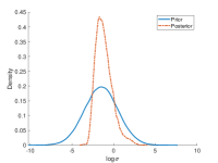
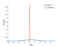
Since we consider choosing the prior distribution from a parameterized family, the target posterior distributions belong to a parameterized family (parameterized by the same prior hyperparameters) as well. We let the importance sampling distribution be the posterior $\pi_{\text{IS}}=\pi_{\text{post}}^{\text{IS}}$ constructed using a specific choice of prior, $\pi_{\text{pr}}^{\text{IS}}$. This $\pi_{\text{pr}}^{\text{IS}}$ is chosen from the same family as the priors in such a way that its high probability region covers that of the family of target priors. See Fig. 1 for an illustration, for the case of Gaussian priors. We then consider

$$\pi_{\text{post}}^{\text{IS}}({\mathchoice{\mbox{\boldmath$\displaystyle{\theta}$}}{\mbox{\boldmath$\textstyle{\theta}$}}{\mbox{\boldmath$\scriptstyle{\theta}$}}{\mbox{\boldmath$\scriptscriptstyle{\theta}$}}}|{\mathchoice{\mbox{\boldmath$\displaystyle{d}$}}{\mbox{\boldmath$\textstyle{d}$}}{\mbox{\boldmath$\scriptstyle{d}$}}{\mbox{\boldmath$\scriptscriptstyle{d}$}}})\propto\pi_{\mathrm{like}}({\mathchoice{\mbox{\boldmath$\displaystyle{d}$}}{\mbox{\boldmath$\textstyle{d}$}}{\mbox{\boldmath$\scriptstyle{d}$}}{\mbox{\boldmath$\scriptscriptstyle{d}$}}}|{\mathchoice{\mbox{\boldmath$\displaystyle{\theta}$}}{\mbox{\boldmath$\textstyle{\theta}$}}{\mbox{\boldmath$\scriptstyle{\theta}$}}{\mbox{\boldmath$\scriptscriptstyle{\theta}$}}})\times\pi_{\text{pr}}^{\text{IS}}({\mathchoice{\mbox{\boldmath$\displaystyle{\theta}$}}{\mbox{\boldmath$\textstyle{\theta}$}}{\mbox{\boldmath$\scriptstyle{\theta}$}}{\mbox{\boldmath$\scriptscriptstyle{\theta}$}}}).$$ (12)

Importance sampling often breaks down if the importance sampling distribution fails to cover the density of the target, especially when the target distribution has a heavy tail. As noted in our computational results, choosing a prior that “covers” all the target priors typically results in a suitable importance sampling posterior $\pi_{\text{post}}^{\text{IS}}$. With the present strategy, it is possible to sample from $\pi_{\text{post}}^{\text{IS}}$ with one run of MCMC and gather information for all the target posteriors.

Next, we derive an expression for the estimator (11) when $\pi_{\text{IS}}=\pi_{\text{post}}^{\text{IS}}$. We let ${\mathchoice{\mbox{\boldmath$\displaystyle{\theta}$}}{\mbox{\boldmath$\textstyle{\theta}$}}{\mbox{\boldmath$\scriptstyle{\theta}$}}{\mbox{\boldmath$\scriptscriptstyle{\theta}$}}}_{\text{IS}}$ and $\Gamma_{\text{IS}}$ denote the mean and covariance of $\pi_{\text{pr}}^{\text{IS}}$ while ${\mathchoice{\mbox{\boldmath$\displaystyle{\theta}$}}{\mbox{\boldmath$\textstyle{\theta}$}}{\mbox{\boldmath$\scriptstyle{\theta}$}}{\mbox{\boldmath$\scriptscriptstyle{\theta}$}}}_{\mathchoice{\mbox{\boldmath$\displaystyle{\xi}$}}{\mbox{\boldmath$\textstyle{\xi}$}}{\mbox{\boldmath$\scriptstyle{\xi}$}}{\mbox{\boldmath$\scriptscriptstyle{\xi}$}}}$ and $\Gamma_{\mathchoice{\mbox{\boldmath$\displaystyle{\xi}$}}{\mbox{\boldmath$\textstyle{\xi}$}}{\mbox{\boldmath$\scriptstyle{\xi}$}}{\mbox{\boldmath$\scriptscriptstyle{\xi}$}}}$ will denote the mean and covariance of $\pi_{\text{pr}}^{{\mathchoice{\mbox{\boldmath$\displaystyle{\xi}$}}{\mbox{\boldmath$\textstyle{\xi}$}}{\mbox{\boldmath$\scriptstyle{\xi}$}}{\mbox{\boldmath$\scriptscriptstyle{\xi}$}}}}$. Let $P^{{\mathchoice{\mbox{\boldmath$\displaystyle{\xi}$}}{\mbox{\boldmath$\textstyle{\xi}$}}{\mbox{\boldmath$\scriptstyle{\xi}$}}{\mbox{\boldmath$\scriptscriptstyle{\xi}$}}}}$ and $P^{\text{IS}}$ be the normalization constants that correspond to $\pi_{\text{post}}^{{\mathchoice{\mbox{\boldmath$\displaystyle{\xi}$}}{\mbox{\boldmath$\textstyle{\xi}$}}{\mbox{\boldmath$\scriptstyle{\xi}$}}{\mbox{\boldmath$\scriptscriptstyle{\xi}$}}}}$ and $\pi_{\text{post}}^{\text{IS}}$, respectively:

$$P^{{\mathchoice{\mbox{\boldmath$\displaystyle{\xi}$}}{\mbox{\boldmath$\textstyle{\xi}$}}{\mbox{\boldmath$\scriptstyle{\xi}$}}{\mbox{\boldmath$\scriptscriptstyle{\xi}$}}}}\vcentcolon=\int_{\mathbb{R}^{d}}\pi_{\text{like}}({\mathchoice{\mbox{\boldmath$\displaystyle{d}$}}{\mbox{\boldmath$\textstyle{d}$}}{\mbox{\boldmath$\scriptstyle{d}$}}{\mbox{\boldmath$\scriptscriptstyle{d}$}}}|{\mathchoice{\mbox{\boldmath$\displaystyle{\theta}$}}{\mbox{\boldmath$\textstyle{\theta}$}}{\mbox{\boldmath$\scriptstyle{\theta}$}}{\mbox{\boldmath$\scriptscriptstyle{\theta}$}}})\pi_{\text{pr}}^{{\mathchoice{\mbox{\boldmath$\displaystyle{\xi}$}}{\mbox{\boldmath$\textstyle{\xi}$}}{\mbox{\boldmath$\scriptstyle{\xi}$}}{\mbox{\boldmath$\scriptscriptstyle{\xi}$}}}}({\mathchoice{\mbox{\boldmath$\displaystyle{\theta}$}}{\mbox{\boldmath$\textstyle{\theta}$}}{\mbox{\boldmath$\scriptstyle{\theta}$}}{\mbox{\boldmath$\scriptscriptstyle{\theta}$}}})\,d{\mathchoice{\mbox{\boldmath$\displaystyle{\theta}$}}{\mbox{\boldmath$\textstyle{\theta}$}}{\mbox{\boldmath$\scriptstyle{\theta}$}}{\mbox{\boldmath$\scriptscriptstyle{\theta}$}}},\quad P^{\text{IS}}\vcentcolon=\int_{\mathbb{R}^{d}}\pi_{\text{like}}({\mathchoice{\mbox{\boldmath$\displaystyle{d}$}}{\mbox{\boldmath$\textstyle{d}$}}{\mbox{\boldmath$\scriptstyle{d}$}}{\mbox{\boldmath$\scriptscriptstyle{d}$}}}|{\mathchoice{\mbox{\boldmath$\displaystyle{\theta}$}}{\mbox{\boldmath$\textstyle{\theta}$}}{\mbox{\boldmath$\scriptstyle{\theta}$}}{\mbox{\boldmath$\scriptscriptstyle{\theta}$}}})\pi_{\text{pr}}^{\text{IS}}({\mathchoice{\mbox{\boldmath$\displaystyle{\theta}$}}{\mbox{\boldmath$\textstyle{\theta}$}}{\mbox{\boldmath$\scriptstyle{\theta}$}}{\mbox{\boldmath$\scriptscriptstyle{\theta}$}}})\,d{\mathchoice{\mbox{\boldmath$\displaystyle{\theta}$}}{\mbox{\boldmath$\textstyle{\theta}$}}{\mbox{\boldmath$\scriptstyle{\theta}$}}{\mbox{\boldmath$\scriptscriptstyle{\theta}$}}}.$$ (13)

We can write the importance sampling weights in (10) as

$$w^{{\mathchoice{\mbox{\boldmath$\displaystyle{\xi}$}}{\mbox{\boldmath$\textstyle{\xi}$}}{\mbox{\boldmath$\scriptstyle{\xi}$}}{\mbox{\boldmath$\scriptscriptstyle{\xi}$}}}}({\mathchoice{\mbox{\boldmath$\displaystyle{\theta}$}}{\mbox{\boldmath$\textstyle{\theta}$}}{\mbox{\boldmath$\scriptstyle{\theta}$}}{\mbox{\boldmath$\scriptscriptstyle{\theta}$}}})=\frac{\pi_{\text{post}}^{{\mathchoice{\mbox{\boldmath$\displaystyle{\xi}$}}{\mbox{\boldmath$\textstyle{\xi}$}}{\mbox{\boldmath$\scriptstyle{\xi}$}}{\mbox{\boldmath$\scriptscriptstyle{\xi}$}}}}({\mathchoice{\mbox{\boldmath$\displaystyle{\theta}$}}{\mbox{\boldmath$\textstyle{\theta}$}}{\mbox{\boldmath$\scriptstyle{\theta}$}}{\mbox{\boldmath$\scriptscriptstyle{\theta}$}}})}{\pi_{\text{post}}^{\text{IS}}{\mathchoice{\mbox{\boldmath$\displaystyle{\theta}$}}{\mbox{\boldmath$\textstyle{\theta}$}}{\mbox{\boldmath$\scriptstyle{\theta}$}}{\mbox{\boldmath$\scriptscriptstyle{\theta}$}}})}=\frac{\pi_{\text{pr}}^{{\mathchoice{\mbox{\boldmath$\displaystyle{\xi}$}}{\mbox{\boldmath$\textstyle{\xi}$}}{\mbox{\boldmath$\scriptstyle{\xi}$}}{\mbox{\boldmath$\scriptscriptstyle{\xi}$}}}}({\mathchoice{\mbox{\boldmath$\displaystyle{\theta}$}}{\mbox{\boldmath$\textstyle{\theta}$}}{\mbox{\boldmath$\scriptstyle{\theta}$}}{\mbox{\boldmath$\scriptscriptstyle{\theta}$}}})\pi_{\text{like}}({\mathchoice{\mbox{\boldmath$\displaystyle{\theta}$}}{\mbox{\boldmath$\textstyle{\theta}$}}{\mbox{\boldmath$\scriptstyle{\theta}$}}{\mbox{\boldmath$\scriptscriptstyle{\theta}$}}})/P^{{\mathchoice{\mbox{\boldmath$\displaystyle{\xi}$}}{\mbox{\boldmath$\textstyle{\xi}$}}{\mbox{\boldmath$\scriptstyle{\xi}$}}{\mbox{\boldmath$\scriptscriptstyle{\xi}$}}}}}{\pi_{\text{pr}}^{\text{IS}}({\mathchoice{\mbox{\boldmath$\displaystyle{\theta}$}}{\mbox{\boldmath$\textstyle{\theta}$}}{\mbox{\boldmath$\scriptstyle{\theta}$}}{\mbox{\boldmath$\scriptscriptstyle{\theta}$}}})\pi_{\text{like}}({\mathchoice{\mbox{\boldmath$\displaystyle{\theta}$}}{\mbox{\boldmath$\textstyle{\theta}$}}{\mbox{\boldmath$\scriptstyle{\theta}$}}{\mbox{\boldmath$\scriptscriptstyle{\theta}$}}})/P^{\text{IS}}}=\frac{1}{P^{{\mathchoice{\mbox{\boldmath$\displaystyle{\xi}$}}{\mbox{\boldmath$\textstyle{\xi}$}}{\mbox{\boldmath$\scriptstyle{\xi}$}}{\mbox{\boldmath$\scriptscriptstyle{\xi}$}}}}/P^{\text{IS}}}\frac{\pi_{\text{pr}}^{{\mathchoice{\mbox{\boldmath$\displaystyle{\xi}$}}{\mbox{\boldmath$\textstyle{\xi}$}}{\mbox{\boldmath$\scriptstyle{\xi}$}}{\mbox{\boldmath$\scriptscriptstyle{\xi}$}}}}({\mathchoice{\mbox{\boldmath$\displaystyle{\theta}$}}{\mbox{\boldmath$\textstyle{\theta}$}}{\mbox{\boldmath$\scriptstyle{\theta}$}}{\mbox{\boldmath$\scriptscriptstyle{\theta}$}}})}{\pi_{\text{pr}}^{\text{IS}}({\mathchoice{\mbox{\boldmath$\displaystyle{\theta}$}}{\mbox{\boldmath$\textstyle{\theta}$}}{\mbox{\boldmath$\scriptstyle{\theta}$}}{\mbox{\boldmath$\scriptscriptstyle{\theta}$}}})}.$$ (14)

Letting the importance sampling weight in (11) be given by 14, we obtain

$$\int_{\mathbb{R}^{d}}q(\boldsymbol{\theta})\pi_{\text{post}}^{{\mathchoice{\mbox{\boldmath$\displaystyle{\xi}$}}{\mbox{\boldmath$\textstyle{\xi}$}}{\mbox{\boldmath$\scriptstyle{\xi}$}}{\mbox{\boldmath$\scriptscriptstyle{\xi}$}}}}({\mathchoice{\mbox{\boldmath$\displaystyle{\theta}$}}{\mbox{\boldmath$\textstyle{\theta}$}}{\mbox{\boldmath$\scriptstyle{\theta}$}}{\mbox{\boldmath$\scriptscriptstyle{\theta}$}}})\,d{\mathchoice{\mbox{\boldmath$\displaystyle{\theta}$}}{\mbox{\boldmath$\textstyle{\theta}$}}{\mbox{\boldmath$\scriptstyle{\theta}$}}{\mbox{\boldmath$\scriptscriptstyle{\theta}$}}}=\frac{1}{P^{{\mathchoice{\mbox{\boldmath$\displaystyle{\xi}$}}{\mbox{\boldmath$\textstyle{\xi}$}}{\mbox{\boldmath$\scriptstyle{\xi}$}}{\mbox{\boldmath$\scriptscriptstyle{\xi}$}}}}/P^{\text{IS}}}\int_{\mathbb{R}^{d}}q({\mathchoice{\mbox{\boldmath$\displaystyle{\theta}$}}{\mbox{\boldmath$\textstyle{\theta}$}}{\mbox{\boldmath$\scriptstyle{\theta}$}}{\mbox{\boldmath$\scriptscriptstyle{\theta}$}}})\frac{\pi_{\text{pr}}^{{\mathchoice{\mbox{\boldmath$\displaystyle{\xi}$}}{\mbox{\boldmath$\textstyle{\xi}$}}{\mbox{\boldmath$\scriptstyle{\xi}$}}{\mbox{\boldmath$\scriptscriptstyle{\xi}$}}}}({\mathchoice{\mbox{\boldmath$\displaystyle{\theta}$}}{\mbox{\boldmath$\textstyle{\theta}$}}{\mbox{\boldmath$\scriptstyle{\theta}$}}{\mbox{\boldmath$\scriptscriptstyle{\theta}$}}})}{\pi_{\text{pr}}^{\text{IS}}({\mathchoice{\mbox{\boldmath$\displaystyle{\theta}$}}{\mbox{\boldmath$\textstyle{\theta}$}}{\mbox{\boldmath$\scriptstyle{\theta}$}}{\mbox{\boldmath$\scriptscriptstyle{\theta}$}}})}\pi_{\text{post}}^{\text{IS}}({\mathchoice{\mbox{\boldmath$\displaystyle{\theta}$}}{\mbox{\boldmath$\textstyle{\theta}$}}{\mbox{\boldmath$\scriptstyle{\theta}$}}{\mbox{\boldmath$\scriptscriptstyle{\theta}$}}})\,d{\mathchoice{\mbox{\boldmath$\displaystyle{\theta}$}}{\mbox{\boldmath$\textstyle{\theta}$}}{\mbox{\boldmath$\scriptstyle{\theta}$}}{\mbox{\boldmath$\scriptscriptstyle{\theta}$}}}.$$ (15)

Furthermore, we can use the importance sampling distribution to rewrite the ratio of normalization constants $P^{{\mathchoice{\mbox{\boldmath$\displaystyle{\xi}$}}{\mbox{\boldmath$\textstyle{\xi}$}}{\mbox{\boldmath$\scriptstyle{\xi}$}}{\mbox{\boldmath$\scriptscriptstyle{\xi}$}}}}/P^{\text{IS}}$ as

$$\frac{P^{{\mathchoice{\mbox{\boldmath$\displaystyle{\xi}$}}{\mbox{\boldmath$\textstyle{\xi}$}}{\mbox{\boldmath$\scriptstyle{\xi}$}}{\mbox{\boldmath$\scriptscriptstyle{\xi}$}}}}}{P^{\text{IS}}}= \frac{1}{P^{\text{IS}}}\int_{\mathbb{R}^{d}}\pi_{\text{like}}({\mathchoice{\mbox{\boldmath$\displaystyle{d}$}}{\mbox{\boldmath$\textstyle{d}$}}{\mbox{\boldmath$\scriptstyle{d}$}}{\mbox{\boldmath$\scriptscriptstyle{d}$}}}|{\mathchoice{\mbox{\boldmath$\displaystyle{\theta}$}}{\mbox{\boldmath$\textstyle{\theta}$}}{\mbox{\boldmath$\scriptstyle{\theta}$}}{\mbox{\boldmath$\scriptscriptstyle{\theta}$}}})\pi_{\text{pr}}^{{\mathchoice{\mbox{\boldmath$\displaystyle{\xi}$}}{\mbox{\boldmath$\textstyle{\xi}$}}{\mbox{\boldmath$\scriptstyle{\xi}$}}{\mbox{\boldmath$\scriptscriptstyle{\xi}$}}}}({\mathchoice{\mbox{\boldmath$\displaystyle{\theta}$}}{\mbox{\boldmath$\textstyle{\theta}$}}{\mbox{\boldmath$\scriptstyle{\theta}$}}{\mbox{\boldmath$\scriptscriptstyle{\theta}$}}})\,d{\mathchoice{\mbox{\boldmath$\displaystyle{\theta}$}}{\mbox{\boldmath$\textstyle{\theta}$}}{\mbox{\boldmath$\scriptstyle{\theta}$}}{\mbox{\boldmath$\scriptscriptstyle{\theta}$}}}$$

$$= \frac{1}{P^{\text{IS}}}\int_{\mathbb{R}^{d}}\pi_{\text{like}}({\mathchoice{\mbox{\boldmath$\displaystyle{d}$}}{\mbox{\boldmath$\textstyle{d}$}}{\mbox{\boldmath$\scriptstyle{d}$}}{\mbox{\boldmath$\scriptscriptstyle{d}$}}}|{\mathchoice{\mbox{\boldmath$\displaystyle{\theta}$}}{\mbox{\boldmath$\textstyle{\theta}$}}{\mbox{\boldmath$\scriptstyle{\theta}$}}{\mbox{\boldmath$\scriptscriptstyle{\theta}$}}})\pi_{\text{pr}}^{{\mathchoice{\mbox{\boldmath$\displaystyle{\xi}$}}{\mbox{\boldmath$\textstyle{\xi}$}}{\mbox{\boldmath$\scriptstyle{\xi}$}}{\mbox{\boldmath$\scriptscriptstyle{\xi}$}}}}({\mathchoice{\mbox{\boldmath$\displaystyle{\theta}$}}{\mbox{\boldmath$\textstyle{\theta}$}}{\mbox{\boldmath$\scriptstyle{\theta}$}}{\mbox{\boldmath$\scriptscriptstyle{\theta}$}}})\frac{P^{\text{IS}}}{\pi_{\text{like}}({\mathchoice{\mbox{\boldmath$\displaystyle{d}$}}{\mbox{\boldmath$\textstyle{d}$}}{\mbox{\boldmath$\scriptstyle{d}$}}{\mbox{\boldmath$\scriptscriptstyle{d}$}}}|{\mathchoice{\mbox{\boldmath$\displaystyle{\theta}$}}{\mbox{\boldmath$\textstyle{\theta}$}}{\mbox{\boldmath$\scriptstyle{\theta}$}}{\mbox{\boldmath$\scriptscriptstyle{\theta}$}}})\pi_{\text{pr}}^{\text{IS}}({\mathchoice{\mbox{\boldmath$\displaystyle{\theta}$}}{\mbox{\boldmath$\textstyle{\theta}$}}{\mbox{\boldmath$\scriptstyle{\theta}$}}{\mbox{\boldmath$\scriptscriptstyle{\theta}$}}})}\pi_{\text{post}}^{\text{IS}}({\mathchoice{\mbox{\boldmath$\displaystyle{\theta}$}}{\mbox{\boldmath$\textstyle{\theta}$}}{\mbox{\boldmath$\scriptstyle{\theta}$}}{\mbox{\boldmath$\scriptscriptstyle{\theta}$}}})\,d{\mathchoice{\mbox{\boldmath$\displaystyle{\theta}$}}{\mbox{\boldmath$\textstyle{\theta}$}}{\mbox{\boldmath$\scriptstyle{\theta}$}}{\mbox{\boldmath$\scriptscriptstyle{\theta}$}}}$$

$$= \frac{1}{P^{\text{IS}}}\int_{\mathbb{R}^{d}}P^{\text{IS}}\frac{\pi_{\text{pr}}^{{\mathchoice{\mbox{\boldmath$\displaystyle{\xi}$}}{\mbox{\boldmath$\textstyle{\xi}$}}{\mbox{\boldmath$\scriptstyle{\xi}$}}{\mbox{\boldmath$\scriptscriptstyle{\xi}$}}}}({\mathchoice{\mbox{\boldmath$\displaystyle{\theta}$}}{\mbox{\boldmath$\textstyle{\theta}$}}{\mbox{\boldmath$\scriptstyle{\theta}$}}{\mbox{\boldmath$\scriptscriptstyle{\theta}$}}})}{\pi_{\text{pr}}^{\text{IS}}({\mathchoice{\mbox{\boldmath$\displaystyle{\theta}$}}{\mbox{\boldmath$\textstyle{\theta}$}}{\mbox{\boldmath$\scriptstyle{\theta}$}}{\mbox{\boldmath$\scriptscriptstyle{\theta}$}}})}\pi_{\text{post}}^{\text{IS}}({\mathchoice{\mbox{\boldmath$\displaystyle{\theta}$}}{\mbox{\boldmath$\textstyle{\theta}$}}{\mbox{\boldmath$\scriptstyle{\theta}$}}{\mbox{\boldmath$\scriptscriptstyle{\theta}$}}})\,d{\mathchoice{\mbox{\boldmath$\displaystyle{\theta}$}}{\mbox{\boldmath$\textstyle{\theta}$}}{\mbox{\boldmath$\scriptstyle{\theta}$}}{\mbox{\boldmath$\scriptscriptstyle{\theta}$}}}$$

$$= \int_{\mathbb{R}^{d}}\frac{\pi_{\text{pr}}^{{\mathchoice{\mbox{\boldmath$\displaystyle{\xi}$}}{\mbox{\boldmath$\textstyle{\xi}$}}{\mbox{\boldmath$\scriptstyle{\xi}$}}{\mbox{\boldmath$\scriptscriptstyle{\xi}$}}}}({\mathchoice{\mbox{\boldmath$\displaystyle{\theta}$}}{\mbox{\boldmath$\textstyle{\theta}$}}{\mbox{\boldmath$\scriptstyle{\theta}$}}{\mbox{\boldmath$\scriptscriptstyle{\theta}$}}})}{\pi_{\text{pr}}^{\text{IS}}({\mathchoice{\mbox{\boldmath$\displaystyle{\theta}$}}{\mbox{\boldmath$\textstyle{\theta}$}}{\mbox{\boldmath$\scriptstyle{\theta}$}}{\mbox{\boldmath$\scriptscriptstyle{\theta}$}}})}\pi_{\text{post}}^{\text{IS}}({\mathchoice{\mbox{\boldmath$\displaystyle{\theta}$}}{\mbox{\boldmath$\textstyle{\theta}$}}{\mbox{\boldmath$\scriptstyle{\theta}$}}{\mbox{\boldmath$\scriptscriptstyle{\theta}$}}})\,d{\mathchoice{\mbox{\boldmath$\displaystyle{\theta}$}}{\mbox{\boldmath$\textstyle{\theta}$}}{\mbox{\boldmath$\scriptstyle{\theta}$}}{\mbox{\boldmath$\scriptscriptstyle{\theta}$}}}.$$ (16)

Combining the expressions (15) and 16 yields the estimator

$$F({\mathchoice{\mbox{\boldmath$\displaystyle{\xi}$}}{\mbox{\boldmath$\textstyle{\xi}$}}{\mbox{\boldmath$\scriptstyle{\xi}$}}{\mbox{\boldmath$\scriptscriptstyle{\xi}$}}})=\int_{\mathbb{R}^{d}}q(\boldsymbol{\theta})\pi_{\text{post}}^{{\mathchoice{\mbox{\boldmath$\displaystyle{\xi}$}}{\mbox{\boldmath$\textstyle{\xi}$}}{\mbox{\boldmath$\scriptstyle{\xi}$}}{\mbox{\boldmath$\scriptscriptstyle{\xi}$}}}}({\mathchoice{\mbox{\boldmath$\displaystyle{\theta}$}}{\mbox{\boldmath$\textstyle{\theta}$}}{\mbox{\boldmath$\scriptstyle{\theta}$}}{\mbox{\boldmath$\scriptscriptstyle{\theta}$}}})\,d{\mathchoice{\mbox{\boldmath$\displaystyle{\theta}$}}{\mbox{\boldmath$\textstyle{\theta}$}}{\mbox{\boldmath$\scriptstyle{\theta}$}}{\mbox{\boldmath$\scriptscriptstyle{\theta}$}}}\approx\frac{1}{C({\mathchoice{\mbox{\boldmath$\displaystyle{\theta}$}}{\mbox{\boldmath$\textstyle{\theta}$}}{\mbox{\boldmath$\scriptstyle{\theta}$}}{\mbox{\boldmath$\scriptscriptstyle{\theta}$}}}_{1},\ldots,{\mathchoice{\mbox{\boldmath$\displaystyle{\theta}$}}{\mbox{\boldmath$\textstyle{\theta}$}}{\mbox{\boldmath$\scriptstyle{\theta}$}}{\mbox{\boldmath$\scriptscriptstyle{\theta}$}}}_{M})}\sum_{i=1}^{M}q(\boldsymbol{\theta}_{i})\frac{\pi_{\text{pr}}^{{\mathchoice{\mbox{\boldmath$\displaystyle{\xi}$}}{\mbox{\boldmath$\textstyle{\xi}$}}{\mbox{\boldmath$\scriptstyle{\xi}$}}{\mbox{\boldmath$\scriptscriptstyle{\xi}$}}}}({\mathchoice{\mbox{\boldmath$\displaystyle{\theta}$}}{\mbox{\boldmath$\textstyle{\theta}$}}{\mbox{\boldmath$\scriptstyle{\theta}$}}{\mbox{\boldmath$\scriptscriptstyle{\theta}$}}}_{i})}{\pi_{\text{pr}}^{\text{IS}}(\boldsymbol{\theta}_{i})},\quad{\mathchoice{\mbox{\boldmath$\displaystyle{\theta}$}}{\mbox{\boldmath$\textstyle{\theta}$}}{\mbox{\boldmath$\scriptstyle{\theta}$}}{\mbox{\boldmath$\scriptscriptstyle{\theta}$}}}_{i}\sim\pi_{\text{post}}^{\text{IS}},$$ (17)

where $C({\mathchoice{\mbox{\boldmath$\displaystyle{\theta}$}}{\mbox{\boldmath$\textstyle{\theta}$}}{\mbox{\boldmath$\scriptstyle{\theta}$}}{\mbox{\boldmath$\scriptscriptstyle{\theta}$}}}_{1},\ldots,{\mathchoice{\mbox{\boldmath$\displaystyle{\theta}$}}{\mbox{\boldmath$\textstyle{\theta}$}}{\mbox{\boldmath$\scriptstyle{\theta}$}}{\mbox{\boldmath$\scriptscriptstyle{\theta}$}}}_{M})=\sum_{i=1}^{M}\frac{\pi_{\text{pr}}^{{\mathchoice{\mbox{\boldmath$\displaystyle{\xi}$}}{\mbox{\boldmath$\textstyle{\xi}$}}{\mbox{\boldmath$\scriptstyle{\xi}$}}{\mbox{\boldmath$\scriptscriptstyle{\xi}$}}}}({\mathchoice{\mbox{\boldmath$\displaystyle{\theta}$}}{\mbox{\boldmath$\textstyle{\theta}$}}{\mbox{\boldmath$\scriptstyle{\theta}$}}{\mbox{\boldmath$\scriptscriptstyle{\theta}$}}}_{i})}{\pi_{\text{pr}}^{\text{IS}}({\mathchoice{\mbox{\boldmath$\displaystyle{\theta}$}}{\mbox{\boldmath$\textstyle{\theta}$}}{\mbox{\boldmath$\scriptstyle{\theta}$}}{\mbox{\boldmath$\scriptscriptstyle{\theta}$}}}_{i})}$ is from the estimator of 16. Note that in the case of Gaussian priors,

$$\frac{\pi_{\text{pr}}^{{\mathchoice{\mbox{\boldmath$\displaystyle{\xi}$}}{\mbox{\boldmath$\textstyle{\xi}$}}{\mbox{\boldmath$\scriptstyle{\xi}$}}{\mbox{\boldmath$\scriptscriptstyle{\xi}$}}}}({\mathchoice{\mbox{\boldmath$\displaystyle{\theta}$}}{\mbox{\boldmath$\textstyle{\theta}$}}{\mbox{\boldmath$\scriptstyle{\theta}$}}{\mbox{\boldmath$\scriptscriptstyle{\theta}$}}})}{\pi_{\text{pr}}^{\text{IS}}(\boldsymbol{\theta})}=\mathrm{exp}\Big{[}\frac{1}{2}\left(({\mathchoice{\mbox{\boldmath$\displaystyle{\theta}$}}{\mbox{\boldmath$\textstyle{\theta}$}}{\mbox{\boldmath$\scriptstyle{\theta}$}}{\mbox{\boldmath$\scriptscriptstyle{\theta}$}}}_{\mathrm{IS}}-\boldsymbol{\theta})^{\top}\Gamma_{\mathrm{IS}}^{-1}(\boldsymbol{\theta}_{\mathrm{IS}}-\boldsymbol{\theta})-(\boldsymbol{\theta}_{\mathchoice{\mbox{\boldmath$\displaystyle{\xi}$}}{\mbox{\boldmath$\textstyle{\xi}$}}{\mbox{\boldmath$\scriptstyle{\xi}$}}{\mbox{\boldmath$\scriptscriptstyle{\xi}$}}}-\boldsymbol{\theta})^{\top}\Gamma_{\mathchoice{\mbox{\boldmath$\displaystyle{\xi}$}}{\mbox{\boldmath$\textstyle{\xi}$}}{\mbox{\boldmath$\scriptstyle{\xi}$}}{\mbox{\boldmath$\scriptscriptstyle{\xi}$}}}^{-1}(\boldsymbol{\theta}_{\mathchoice{\mbox{\boldmath$\displaystyle{\xi}$}}{\mbox{\boldmath$\textstyle{\xi}$}}{\mbox{\boldmath$\scriptstyle{\xi}$}}{\mbox{\boldmath$\scriptscriptstyle{\xi}$}}}-\boldsymbol{\theta})\right)\Big{]}.$$ (18)

There are some diagnostics for evaluating the effectiveness of a sample set from the importance sampling distribution [22]. We use effective sample size in our experiments. A large effective sample size is desirable as it indicates small variation in the estimator (15). For a given $\textstyle{\xi}$, the effective sample size is

$$n_{\text{E}}^{\mathchoice{\mbox{\boldmath$\displaystyle{\xi}$}}{\mbox{\boldmath$\textstyle{\xi}$}}{\mbox{\boldmath$\scriptstyle{\xi}$}}{\mbox{\boldmath$\scriptscriptstyle{\xi}$}}}\vcentcolon=\frac{\big{(}\sum_{i=1}^{M}w^{\mathchoice{\mbox{\boldmath$\displaystyle{\xi}$}}{\mbox{\boldmath$\textstyle{\xi}$}}{\mbox{\boldmath$\scriptstyle{\xi}$}}{\mbox{\boldmath$\scriptscriptstyle{\xi}$}}}({\mathchoice{\mbox{\boldmath$\displaystyle{\theta}$}}{\mbox{\boldmath$\textstyle{\theta}$}}{\mbox{\boldmath$\scriptstyle{\theta}$}}{\mbox{\boldmath$\scriptscriptstyle{\theta}$}}}_{i})\big{)}^{2}}{\sum_{i=1}^{M}w^{\mathchoice{\mbox{\boldmath$\displaystyle{\xi}$}}{\mbox{\boldmath$\textstyle{\xi}$}}{\mbox{\boldmath$\scriptstyle{\xi}$}}{\mbox{\boldmath$\scriptscriptstyle{\xi}$}}}({\mathchoice{\mbox{\boldmath$\displaystyle{\theta}$}}{\mbox{\boldmath$\textstyle{\theta}$}}{\mbox{\boldmath$\scriptstyle{\theta}$}}{\mbox{\boldmath$\scriptscriptstyle{\theta}$}}}_{i})^{2}},\quad{\mathchoice{\mbox{\boldmath$\displaystyle{\theta}$}}{\mbox{\boldmath$\textstyle{\theta}$}}{\mbox{\boldmath$\scriptstyle{\theta}$}}{\mbox{\boldmath$\scriptscriptstyle{\theta}$}}}_{i}\sim\pi_{\text{post}}^{\text{IS}}.$$ (19)

Recall from (14) that we can rewrite $w^{\mathchoice{\mbox{\boldmath$\displaystyle{\xi}$}}{\mbox{\boldmath$\textstyle{\xi}$}}{\mbox{\boldmath$\scriptstyle{\xi}$}}{\mbox{\boldmath$\scriptscriptstyle{\xi}$}}}=\frac{\pi_{\text{post}}^{{\mathchoice{\mbox{\boldmath$\displaystyle{\xi}$}}{\mbox{\boldmath$\textstyle{\xi}$}}{\mbox{\boldmath$\scriptstyle{\xi}$}}{\mbox{\boldmath$\scriptscriptstyle{\xi}$}}}}}{\pi_{\text{post}}^{\text{IS}}}=\frac{1}{P^{\mathchoice{\mbox{\boldmath$\displaystyle{\xi}$}}{\mbox{\boldmath$\textstyle{\xi}$}}{\mbox{\boldmath$\scriptstyle{\xi}$}}{\mbox{\boldmath$\scriptscriptstyle{\xi}$}}}/P^{\text{IS}}}\frac{\pi_{\text{pr}}^{{\mathchoice{\mbox{\boldmath$\displaystyle{\xi}$}}{\mbox{\boldmath$\textstyle{\xi}$}}{\mbox{\boldmath$\scriptstyle{\xi}$}}{\mbox{\boldmath$\scriptscriptstyle{\xi}$}}}}}{\pi_{\text{pr}}^{\text{IS}}}$, Then, we can write (19) as

$$n_{\text{E}}^{\mathchoice{\mbox{\boldmath$\displaystyle{\xi}$}}{\mbox{\boldmath$\textstyle{\xi}$}}{\mbox{\boldmath$\scriptstyle{\xi}$}}{\mbox{\boldmath$\scriptscriptstyle{\xi}$}}}=\frac{\big{(}\sum_{i=1}^{M}\frac{\pi_{\text{post}}^{{\mathchoice{\mbox{\boldmath$\displaystyle{\xi}$}}{\mbox{\boldmath$\textstyle{\xi}$}}{\mbox{\boldmath$\scriptstyle{\xi}$}}{\mbox{\boldmath$\scriptscriptstyle{\xi}$}}}}({\mathchoice{\mbox{\boldmath$\displaystyle{\theta}$}}{\mbox{\boldmath$\textstyle{\theta}$}}{\mbox{\boldmath$\scriptstyle{\theta}$}}{\mbox{\boldmath$\scriptscriptstyle{\theta}$}}}_{i})}{\pi_{\text{post}}^{\text{IS}}({\mathchoice{\mbox{\boldmath$\displaystyle{\theta}$}}{\mbox{\boldmath$\textstyle{\theta}$}}{\mbox{\boldmath$\scriptstyle{\theta}$}}{\mbox{\boldmath$\scriptscriptstyle{\theta}$}}}_{i})}\big{)}^{2}}{\sum_{i=1}^{M}\big{(}\frac{\pi_{\text{post}}^{{\mathchoice{\mbox{\boldmath$\displaystyle{\xi}$}}{\mbox{\boldmath$\textstyle{\xi}$}}{\mbox{\boldmath$\scriptstyle{\xi}$}}{\mbox{\boldmath$\scriptscriptstyle{\xi}$}}}}({\mathchoice{\mbox{\boldmath$\displaystyle{\theta}$}}{\mbox{\boldmath$\textstyle{\theta}$}}{\mbox{\boldmath$\scriptstyle{\theta}$}}{\mbox{\boldmath$\scriptscriptstyle{\theta}$}}}_{i})}{\pi_{\text{post}}^{\text{IS}}({\mathchoice{\mbox{\boldmath$\displaystyle{\theta}$}}{\mbox{\boldmath$\textstyle{\theta}$}}{\mbox{\boldmath$\scriptstyle{\theta}$}}{\mbox{\boldmath$\scriptscriptstyle{\theta}$}}}_{i})}\big{)}^{2}}=\frac{\big{(}\sum_{i=1}^{M}\frac{1}{P^{\mathchoice{\mbox{\boldmath$\displaystyle{\xi}$}}{\mbox{\boldmath$\textstyle{\xi}$}}{\mbox{\boldmath$\scriptstyle{\xi}$}}{\mbox{\boldmath$\scriptscriptstyle{\xi}$}}}/P^{\text{IS}}}\frac{\pi_{\text{pr}}^{{\mathchoice{\mbox{\boldmath$\displaystyle{\xi}$}}{\mbox{\boldmath$\textstyle{\xi}$}}{\mbox{\boldmath$\scriptstyle{\xi}$}}{\mbox{\boldmath$\scriptscriptstyle{\xi}$}}}}({\mathchoice{\mbox{\boldmath$\displaystyle{\theta}$}}{\mbox{\boldmath$\textstyle{\theta}$}}{\mbox{\boldmath$\scriptstyle{\theta}$}}{\mbox{\boldmath$\scriptscriptstyle{\theta}$}}}_{i})}{\pi_{\text{pr}}^{\text{IS}}({\mathchoice{\mbox{\boldmath$\displaystyle{\theta}$}}{\mbox{\boldmath$\textstyle{\theta}$}}{\mbox{\boldmath$\scriptstyle{\theta}$}}{\mbox{\boldmath$\scriptscriptstyle{\theta}$}}}_{i})}\big{)}^{2}}{\sum_{i=1}^{M}\big{(}\frac{1}{P^{\mathchoice{\mbox{\boldmath$\displaystyle{\xi}$}}{\mbox{\boldmath$\textstyle{\xi}$}}{\mbox{\boldmath$\scriptstyle{\xi}$}}{\mbox{\boldmath$\scriptscriptstyle{\xi}$}}}/P^{\text{IS}}}\frac{\pi_{\text{pr}}^{{\mathchoice{\mbox{\boldmath$\displaystyle{\xi}$}}{\mbox{\boldmath$\textstyle{\xi}$}}{\mbox{\boldmath$\scriptstyle{\xi}$}}{\mbox{\boldmath$\scriptscriptstyle{\xi}$}}}}({\mathchoice{\mbox{\boldmath$\displaystyle{\theta}$}}{\mbox{\boldmath$\textstyle{\theta}$}}{\mbox{\boldmath$\scriptstyle{\theta}$}}{\mbox{\boldmath$\scriptscriptstyle{\theta}$}}}_{i})}{\pi_{\text{pr}}^{\text{IS}}({\mathchoice{\mbox{\boldmath$\displaystyle{\theta}$}}{\mbox{\boldmath$\textstyle{\theta}$}}{\mbox{\boldmath$\scriptstyle{\theta}$}}{\mbox{\boldmath$\scriptscriptstyle{\theta}$}}}_{i})}\big{)}^{2}}=\frac{\big{(}\sum_{i=1}^{M}\frac{\pi_{\text{pr}}^{{\mathchoice{\mbox{\boldmath$\displaystyle{\xi}$}}{\mbox{\boldmath$\textstyle{\xi}$}}{\mbox{\boldmath$\scriptstyle{\xi}$}}{\mbox{\boldmath$\scriptscriptstyle{\xi}$}}}}({\mathchoice{\mbox{\boldmath$\displaystyle{\theta}$}}{\mbox{\boldmath$\textstyle{\theta}$}}{\mbox{\boldmath$\scriptstyle{\theta}$}}{\mbox{\boldmath$\scriptscriptstyle{\theta}$}}}_{i})}{\pi_{\text{pr}}^{\text{IS}}({\mathchoice{\mbox{\boldmath$\displaystyle{\theta}$}}{\mbox{\boldmath$\textstyle{\theta}$}}{\mbox{\boldmath$\scriptstyle{\theta}$}}{\mbox{\boldmath$\scriptscriptstyle{\theta}$}}}_{i})}\big{)}^{2}}{\sum_{i=1}^{M}\big{(}\frac{\pi_{\text{pr}}^{{\mathchoice{\mbox{\boldmath$\displaystyle{\xi}$}}{\mbox{\boldmath$\textstyle{\xi}$}}{\mbox{\boldmath$\scriptstyle{\xi}$}}{\mbox{\boldmath$\scriptscriptstyle{\xi}$}}}}({\mathchoice{\mbox{\boldmath$\displaystyle{\theta}$}}{\mbox{\boldmath$\textstyle{\theta}$}}{\mbox{\boldmath$\scriptstyle{\theta}$}}{\mbox{\boldmath$\scriptscriptstyle{\theta}$}}}_{i})}{\pi_{\text{pr}}^{\text{IS}}({\mathchoice{\mbox{\boldmath$\displaystyle{\theta}$}}{\mbox{\boldmath$\textstyle{\theta}$}}{\mbox{\boldmath$\scriptstyle{\theta}$}}{\mbox{\boldmath$\scriptscriptstyle{\theta}$}}}_{i})}\big{)}^{2}}.$$ (20)

In practice, we assess the suitability of $\pi_{\text{post}}^{\text{IS}}$ as an importance sampling distribution by examining the distribution of $n_{\text{E}}^{\mathchoice{\mbox{\boldmath$\displaystyle{\xi}$}}{\mbox{\boldmath$\textstyle{\xi}$}}{\mbox{\boldmath$\scriptstyle{\xi}$}}{\mbox{\boldmath$\scriptscriptstyle{\xi}$}}}$ for an ensemble of realizations of $\xi$. This is illustrated in our computational results in Section 5.

4.2 Algorithm for GSA of moment based HS maps

We approximate $F_{\mathrm{mean}}(\boldsymbol{\xi})$ and $F_{\mathrm{var}}(\boldsymbol{\xi})$ using (17). When estimating their Sobol’ indices, we opt for the surrogate-assisted approach. Because (17) provides us with noisy evaluations of $F_{\mathrm{mean}}(\boldsymbol{\xi})$ and $F_{\mathrm{var}}(\boldsymbol{\xi})$, estimating Sobol’ indices by the double-loop sampling approach can give poor results. Regression-based surrogate methods are well-suited here. We employ sparse regression PCE and sparse-weight ELM, discussed in Section 3. In Algorithm 1, we detail the proposed framework for variance-based GSA of (6). Samples from one MCMC run are used to estimate, by importance sampling, $F(\boldsymbol{\xi})$ for selected realizations of $\boldsymbol{\xi}$. Sample realizations of $\textstyle{\xi}$ are generated by Latin hypercube sampling (LHS) [47, 48]. . These samples serve as a training set for building surrogate models of $F(\boldsymbol{\xi})$ for GSA, as discussed in Section 3. The purpose of using two different surrogate methods is to help gain further confidence in the computed results.

Algorithm 1 GSA with respect to uncertain prior hyperparameters via importance sampling

Input: (i) Likelihood PDF $\pi_{\mathrm{like}}({\mathchoice{\mbox{\boldmath$\displaystyle{d}$}}{\mbox{\boldmath$\textstyle{d}$}}{\mbox{\boldmath$\scriptstyle{d}$}}{\mbox{\boldmath$\scriptscriptstyle{d}$}}}|{\mathchoice{\mbox{\boldmath$\displaystyle{\theta}$}}{\mbox{\boldmath$\textstyle{\theta}$}}{\mbox{\boldmath$\scriptstyle{\theta}$}}{\mbox{\boldmath$\scriptscriptstyle{\theta}$}}})$ (ii) Hyperparameter-dependent prior PDF $\pi_{\text{pr}}^{{\mathchoice{\mbox{\boldmath$\displaystyle{\xi}$}}{\mbox{\boldmath$\textstyle{\xi}$}}{\mbox{\boldmath$\scriptstyle{\xi}$}}{\mbox{\boldmath$\scriptscriptstyle{\xi}$}}}}(\boldsymbol{\theta})$ (iii) Importance sampling prior PDF $\pi_{\text{pr}}^{\text{IS}}(\boldsymbol{\theta})$ (iv) Collection of hyperparameter samples $\{\boldsymbol{\xi}_{k}\}_{k=1}^{N}$ (v) QoI function $q(\boldsymbol{\theta})$ (vi) Monte Carlo sample size $M$

Output: (i) First-order Sobol’ indices (ii) Total Sobol’ indices

1:Perform MCMC to generate samples, $\{\boldsymbol{\theta}_{i}\}_{i=1}^{M}$, from $\pi_{\text{post}}^{\text{IS}}$, of which $\widehat{M}$ are distinct

2:for $i=1,\dots,\widehat{M}$ do

3:     Compute and store $q(\boldsymbol{\theta}_{i})$

4:     Compute and store $\pi_{\text{pr}}^{\text{IS}}(\boldsymbol{\theta}_{i})$

5:     for $k=1,\dots,N$ do

6:         Compute and store $\pi_{\text{pr}}^{{\mathchoice{\mbox{\boldmath$\displaystyle{\xi}$}}{\mbox{\boldmath$\textstyle{\xi}$}}{\mbox{\boldmath$\scriptstyle{\xi}$}}{\mbox{\boldmath$\scriptscriptstyle{\xi}$}}}_{k}}(\boldsymbol{\theta}_{i})$

7:     end for

8:end for

9:for $k=1,\dots,N$ do

10:     Approximate $F(\boldsymbol{\xi}_{k})$ in (6) using the estimator (17) with $\{(q(\boldsymbol{\theta}_{i}),\pi_{\text{pr}}^{{\mathchoice{\mbox{\boldmath$\displaystyle{\xi}$}}{\mbox{\boldmath$\textstyle{\xi}$}}{\mbox{\boldmath$\scriptstyle{\xi}$}}{\mbox{\boldmath$\scriptscriptstyle{\xi}$}}}_{k}}(\boldsymbol{\theta}_{i}),\pi_{\text{pr}}^{\text{IS}}(\boldsymbol{\theta}_{i})\}_{i=1}^{M}$

11:end for

12:Compute a surrogate model $\widehat{F}$ for $F$, using the samples $\{(\boldsymbol{\xi}_{k},F(\boldsymbol{\xi}_{k})\}_{k=1}^{N}$

13:Estimate first-order and total Sobol’ indices of $\widehat{F}$

Under the assumption that the model and QoI $q$ are expensive to evaluate, Algorithm 1 incurs most of its cost during the MCMC sampling stage. In this work, we use the delayed-rejection adaptive Metropolis (DRAM) [49, 50, 28] algorithm to perform MCMC. With delayed-rejection, each MCMC stage can include up to a fixed number of extra delayed-rejection steps. Each of these steps requires us to evaluate the model an additional time. Typically, one initially runs MCMC for $M_{\text{burn}}$ burn-in stages. These burn-in samples are discarded and not included in the set of posterior draws. The cost of running the MCMC stage in Algorithm 1 with DRAM is $\mathcal{O}(M+M_{\text{burn}})$ model evaluations. In the second stage, we evaluate $q$ at the distinct MCMC samples. Because the MCMC samples usually include repeated draws, the number of these QoI evaluations is less than $M$.

4.3 GSA of the MAP point

The MAP point is an important point estimator and studying its sensitivity to prior parameters complements the study of other moment-based HS maps such as the posterior mean or variance. The approach described in Algorithm 1 can be used in cases where $F(\boldsymbol{\xi})$ involves moments of the posterior, as in the case of the mean and variance. On the other hand, evaluating $F_{\mathrm{MAP}}$ requires solving the regularized nonlinear least squares problem (5) for each realization of $\textstyle{\xi}$. No numerical integration is needed. One does not even need to know the normalization constant of the posterior to find its MAP point. While we do not use Algorithm 1 to study $F_{\mathrm{MAP}}$, we evaluate it at the same set of realizations $\{{\mathchoice{\mbox{\boldmath$\displaystyle{\xi}$}}{\mbox{\boldmath$\textstyle{\xi}$}}{\mbox{\boldmath$\scriptstyle{\xi}$}}{\mbox{\boldmath$\scriptscriptstyle{\xi}$}}}_{k}\}_{k=1}^{N}$ used in Algorithm 1. These evaluations are used to build surrogate models for $F_{\text{MAP}}$. The computed surrogate is then used for fast GSA of $F_{\text{MAP}}$.

5 Computational results

In this section, we consider two model inverse problems as testbeds for our proposed approach. Specifically, we use Algorithm 1 for global sensitivity analysis (GSA) of hyperparameter-to-statistic (HS) mappings from the inverse problems under study. These examples are used to examine various aspects of the proposed method. In Section 5.1, we consider a simple linear inverse problem. Specifically, we formulate fitting a line to noisy data as a linear Bayesian inverse problem. In this case, the posterior distribution is known analytically. This means that the HS mappings admit analytical forms, and we can perform GSA without Algorithm 1. This problem serves as a benchmark where we gauge the accuracy of GSA with Algorithm 1 against reference values. The QoI in this example is a quadratic function. For this QoIs, we study the HS mappings for the mean and variance. The Sobol’ indices, approximated using Algorithm 1, of these HS mappings are compared to the true Sobol’ indices. Overall, we note close agreement between the results produced by our method and the analytic results.

Next, we apply our method to a nonlinear Bayesian inverse problem in Section 5.2. The inverse problem is governed by an SEIR model from epidemiology [51, 52]. It exemplifies the type of problem that Algorithm 1 is designed and intended for. Our numerical results provide a unique perspective on the impact of uncertainty in prior hyperparameters. The QoI is the basic reproductive number. We quantify the uncertainty in the mean, variance, and MAP point that is caused by uncertainty in the prior hyperparameters. The Sobol’ indices of the mean, variance, and MAP point HS mappings are computed using Algorithm 1 and highlight the most influential hyperparameters in each case. We use two different surrogate modeling approaches in these computations: one based on sparse polynomial chaos expansions (PCEs) and the other based on sparse weight extreme learning machines (SW-ELMs). The two approaches provide results that match closely.

5.1 Linear Bayesian inverse problem

We consider the problem of fitting a line $y=mt+b$ to noisy measurements $\{(t_{i},y_{i})\}_{i=1}^{4}$ at times $t=0,0.5,1.5,2.5$. The slope $m$ and intercept $b$ are treated as unknown parameters, which we seek to estimate. We cast this problem in a Bayesian framework. This serve to illustrate various properties of our proposed framework.

5.1.1 Bayesian inverse problem setup

Let the inversion parameter vector be denoted by $\boldsymbol{\theta}=\big{[}\begin{array}[]{cc}b&m\end{array}\big{]}^{\top}$. We consider estimation of $\boldsymbol{\theta}$ from

$$\mathbf{{A}}\boldsymbol{\theta}+\boldsymbol{\eta}=\boldsymbol{y},$$ (21)

where Here $\mathbf{{A}}=\left[\begin{array}[]{cccc}1&1&1&1\\ 0&0.5&1.5&2.5\end{array}\right]^{\top}$ is the forward operator, $\textstyle{\eta}$ models measurement noise, and $\textstyle{y}$ is the data.

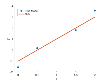
We assume noise at each measurement independently follows the standard normal distribution, i.e., $\eta_{i}\sim\mathcal{N}(0,1)$. The noise covariance is $\boldsymbol{\Gamma}_{\mathrm{noise}}=\mathbf{{I}}_{4\times 4}$. We assume a “ground-truth” parameter vector $\boldsymbol{\theta}_{\text{true}}=[1\;-2]^{\top}$ and generate measurements by adding sampled noise $\eta_{i}$ to $y_{i}=-2t_{i}+1$ for $i=1,\ldots,4$; see Fig. 2.

Figure 2: The true trajectory of the linear model plotted with the noisy measurements at times $t=0,0.5,1.5,2$.

We assume a Gaussian prior distribution $\mathcal{N}({\mathchoice{\mbox{\boldmath$\displaystyle{\theta}$}}{\mbox{\boldmath$\textstyle{\theta}$}}{\mbox{\boldmath$\scriptstyle{\theta}$}}{\mbox{\boldmath$\scriptscriptstyle{\theta}$}}}_{\text{pr}},{\mathchoice{\mbox{\boldmath$\displaystyle{\Gamma}$}}{\mbox{\boldmath$\textstyle{\Gamma}$}}{\mbox{\boldmath$\scriptstyle{\Gamma}$}}{\mbox{\boldmath$\scriptscriptstyle{\Gamma}$}}}_{\text{pr}})$ for the inversion parameters $\textstyle{\theta}$ with

$$\boldsymbol{\theta}_{\mathrm{pr}}=\left[\begin{array}[]{cc}\mu_{b}\\ \mu_{m}\end{array}\right],\quad\boldsymbol{\Gamma}_{\mathrm{pr}}=\left[\begin{array}[]{cc}\sigma_{b}^{2}&0\\ 0&\sigma_{m}^{2}\end{array}\right].$$ (22)

Due to linearity of the parameter-to-observable map and Gaussian prior and noise models, the posterior distribution for $\textstyle{\theta}$ is also Gaussian and explicitly known. It is the Gaussian distribution $\mathcal{N}({\mathchoice{\mbox{\boldmath$\displaystyle{\theta}$}}{\mbox{\boldmath$\textstyle{\theta}$}}{\mbox{\boldmath$\scriptstyle{\theta}$}}{\mbox{\boldmath$\scriptscriptstyle{\theta}$}}}_{\text{post}},{\mathchoice{\mbox{\boldmath$\displaystyle{\Gamma}$}}{\mbox{\boldmath$\textstyle{\Gamma}$}}{\mbox{\boldmath$\scriptstyle{\Gamma}$}}{\mbox{\boldmath$\scriptscriptstyle{\Gamma}$}}}_{\text{post}})$, where

$$\boldsymbol{\Gamma}_{\mathrm{post}}=(\mathbf{{A}}^{\top}\boldsymbol{\Gamma}_{\mathrm{noise}}^{-1}\mathbf{{A}}+\boldsymbol{\Gamma}_{\mathrm{pr}}^{-1})^{-1},\quad\boldsymbol{\theta}_{\mathrm{post}}=\boldsymbol{\Gamma}_{\mathrm{post}}(\mathbf{{A}}^{\top}\boldsymbol{\Gamma}_{\mathrm{noise}}^{-1}\boldsymbol{y}+\boldsymbol{\Gamma}_{\mathrm{pr}}^{-1}\boldsymbol{\theta}_{\mathrm{pr}}).$$ (23)

Since the posterior distribution is Gaussian, the posterior mean and MAP point are the same.

Quantity of interest. We introduce the QoI which depends on the inversion parameters $\textstyle{\theta}$. The QoI is the quadratic form

$$q({\mathchoice{\mbox{\boldmath$\displaystyle{\theta}$}}{\mbox{\boldmath$\textstyle{\theta}$}}{\mbox{\boldmath$\scriptstyle{\theta}$}}{\mbox{\boldmath$\scriptscriptstyle{\theta}$}}})={\mathchoice{\mbox{\boldmath$\displaystyle{\theta}$}}{\mbox{\boldmath$\textstyle{\theta}$}}{\mbox{\boldmath$\scriptstyle{\theta}$}}{\mbox{\boldmath$\scriptscriptstyle{\theta}$}}}^{\top}{\mathchoice{\mbox{\boldmath$\displaystyle{\theta}$}}{\mbox{\boldmath$\textstyle{\theta}$}}{\mbox{\boldmath$\scriptstyle{\theta}$}}{\mbox{\boldmath$\scriptscriptstyle{\theta}$}}}=m^{2}+b^{2},\quad{\mathchoice{\mbox{\boldmath$\displaystyle{\theta}$}}{\mbox{\boldmath$\textstyle{\theta}$}}{\mbox{\boldmath$\scriptstyle{\theta}$}}{\mbox{\boldmath$\scriptscriptstyle{\theta}$}}}\sim\mathcal{N}({\mathchoice{\mbox{\boldmath$\displaystyle{\theta}$}}{\mbox{\boldmath$\textstyle{\theta}$}}{\mbox{\boldmath$\scriptstyle{\theta}$}}{\mbox{\boldmath$\scriptscriptstyle{\theta}$}}}_{\text{post}},{\mathchoice{\mbox{\boldmath$\displaystyle{\Gamma}$}}{\mbox{\boldmath$\textstyle{\Gamma}$}}{\mbox{\boldmath$\scriptstyle{\Gamma}$}}{\mbox{\boldmath$\scriptscriptstyle{\Gamma}$}}}_{\text{post}}).$$ (24)

As $\textstyle{\theta}$ is a Gaussian random variable, we have access to expressions for the first and second moments [53, 54]. of the QoI. We can therefore express the mean and variance of the QoI analytically.

$$\mathbb{E}_{\text{post}}(q)={\mathchoice{\mbox{\boldmath$\displaystyle{\theta}$}}{\mbox{\boldmath$\textstyle{\theta}$}}{\mbox{\boldmath$\scriptstyle{\theta}$}}{\mbox{\boldmath$\scriptscriptstyle{\theta}$}}}_{\text{post}}^{\top}{\mathchoice{\mbox{\boldmath$\displaystyle{\theta}$}}{\mbox{\boldmath$\textstyle{\theta}$}}{\mbox{\boldmath$\scriptstyle{\theta}$}}{\mbox{\boldmath$\scriptscriptstyle{\theta}$}}}_{\text{post}},\quad\text{var}(q)=2\ \text{tr}({\mathchoice{\mbox{\boldmath$\displaystyle{\Gamma}$}}{\mbox{\boldmath$\textstyle{\Gamma}$}}{\mbox{\boldmath$\scriptstyle{\Gamma}$}}{\mbox{\boldmath$\scriptscriptstyle{\Gamma}$}}}_{\text{post}}^{2})+4{\mathchoice{\mbox{\boldmath$\displaystyle{\theta}$}}{\mbox{\boldmath$\textstyle{\theta}$}}{\mbox{\boldmath$\scriptstyle{\theta}$}}{\mbox{\boldmath$\scriptscriptstyle{\theta}$}}}_{\text{post}}^{\top}\Gamma_{\text{post}}{\mathchoice{\mbox{\boldmath$\displaystyle{\theta}$}}{\mbox{\boldmath$\textstyle{\theta}$}}{\mbox{\boldmath$\scriptstyle{\theta}$}}{\mbox{\boldmath$\scriptscriptstyle{\theta}$}}}_{\text{post}}.$$ (25)

Uncertainty in prior hyperparameters. Before building the posterior distribution, we must choose values for the prior hyperparameters are ${\mathchoice{\mbox{\boldmath$\displaystyle{\xi}$}}{\mbox{\boldmath$\textstyle{\xi}$}}{\mbox{\boldmath$\scriptstyle{\xi}$}}{\mbox{\boldmath$\scriptscriptstyle{\xi}$}}}=\big{[}\begin{array}[]{cccc}\mu_{b}&\mu_{m}&\sigma_{b}^{2}&\sigma_{m}^{2}\end{array}\big{]}^{\top}$ that appear in (22). We assume these parameters are specified within some interval around their nominal values and are modeled as independent uniformly distributed random variables. We use a nominal value of 1 for each of the parameters and let the upper and lower bounds of the distributions be $\pm 50\%$ perturbations of the nominal value.

5.1.2 Parameter estimation and importance sampling

To understand how the uncertainty in the prior hyperparameters affects the QoI, we employ Algorithm 1 in Section 4. The first step is to choose a prior $\pi_{\text{pr}}^{\text{IS}}$ to build the importance sampling distribution $\pi_{\text{post}}^{\text{IS}}$. We take $\mathcal{N}({\mathchoice{\mbox{\boldmath$\displaystyle{\theta}$}}{\mbox{\boldmath$\textstyle{\theta}$}}{\mbox{\boldmath$\scriptstyle{\theta}$}}{\mbox{\boldmath$\scriptscriptstyle{\theta}$}}}_{\text{pr}}^{\text{IS}},{\mathchoice{\mbox{\boldmath$\displaystyle{\Gamma}$}}{\mbox{\boldmath$\textstyle{\Gamma}$}}{\mbox{\boldmath$\scriptstyle{\Gamma}$}}{\mbox{\boldmath$\scriptscriptstyle{\Gamma}$}}}_{\text{pr}}^{\text{IS}})$ with

$$\boldsymbol{\theta}_{\mathrm{pr}}=\left[\begin{array}[]{cc}1\\ 1\end{array}\right],\quad\boldsymbol{\Gamma}_{\mathrm{pr}}=\left[\begin{array}[]{cc}1.5^{2}&0\\ 0&1.5^{2}\end{array}\right].$$ (26)

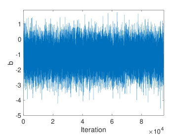
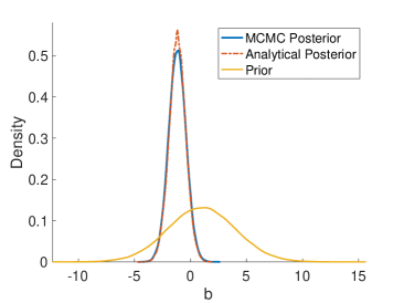
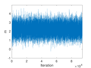
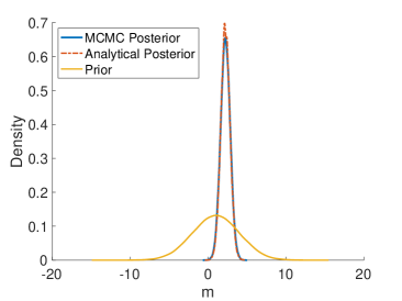
We use the DRAM algorithm, discussed in Section 4, to draw $10^{5}$ samples from $\pi_{\text{post}}^{\text{IS}}$. In Fig. 3, we compare the prior, analytic posterior, and MCMC-constructed posterior marginal distributions of $b$ and $m$.

Figure 3: MCMC chains of the inversion parameters $m$ and $b$ along with corresponding marginal posterior distributions compared to prior distributions.

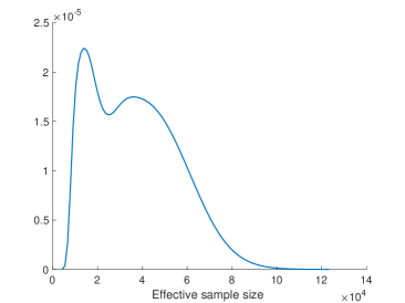
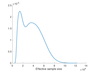
Before we implement Algorithm 1, we evaluate whether $\pi_{\text{post}}^{\text{IS}}$ is an acceptable importance sampling distribution. As discussed in Section 4, we use (20) to compute the effective sample size over the distribution of prior hyperparameters $\textstyle{\xi}$. The distribution of effective sample sizes, given in Fig. 4 (left), shows that $\pi_{\text{post}}^{\text{IS}}$ is an effective importance sampling distribution over many realizations of $\textstyle{\xi}$.

Figure 4: Left: Effective sample size of $\pi_{\text{post}}^{\text{IS}}$ distributed over values $\textstyle{\xi}$. Right: Distribution of $q$ when ${\mathchoice{\mbox{\boldmath$\displaystyle{\theta}$}}{\mbox{\boldmath$\textstyle{\theta}$}}{\mbox{\boldmath$\scriptstyle{\theta}$}}{\mbox{\boldmath$\scriptscriptstyle{\theta}$}}}\sim\pi_{\text{post}}^{\text{IS}}$ compared to when ${\mathchoice{\mbox{\boldmath$\displaystyle{\theta}$}}{\mbox{\boldmath$\textstyle{\theta}$}}{\mbox{\boldmath$\scriptstyle{\theta}$}}{\mbox{\boldmath$\scriptscriptstyle{\theta}$}}}\sim\pi_{\text{post}}^{{\mathchoice{\mbox{\boldmath$\displaystyle{\xi}$}}{\mbox{\boldmath$\textstyle{\xi}$}}{\mbox{\boldmath$\scriptstyle{\xi}$}}{\mbox{\boldmath$\scriptscriptstyle{\xi}$}}}}$ for three realizations of $\textstyle{\xi}$.

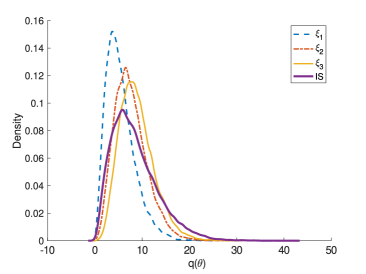
In Fig. 4, we give a further visual of how $\pi_{\text{post}}^{\text{IS}}$ serves as an effective importance sampling distribution. In the right panel, the distribution of $q$, when ${\mathchoice{\mbox{\boldmath$\displaystyle{\theta}$}}{\mbox{\boldmath$\textstyle{\theta}$}}{\mbox{\boldmath$\scriptstyle{\theta}$}}{\mbox{\boldmath$\scriptscriptstyle{\theta}$}}}\sim\pi_{\text{post}}^{\text{IS}}$, is compared to the distributions of $q_{\text{lin}}({\mathchoice{\mbox{\boldmath$\displaystyle{\theta}$}}{\mbox{\boldmath$\textstyle{\theta}$}}{\mbox{\boldmath$\scriptstyle{\theta}$}}{\mbox{\boldmath$\scriptscriptstyle{\theta}$}}})$ when ${\mathchoice{\mbox{\boldmath$\displaystyle{\theta}$}}{\mbox{\boldmath$\textstyle{\theta}$}}{\mbox{\boldmath$\scriptstyle{\theta}$}}{\mbox{\boldmath$\scriptscriptstyle{\theta}$}}}\sim\pi_{\text{post}}^{{\mathchoice{\mbox{\boldmath$\displaystyle{\xi}$}}{\mbox{\boldmath$\textstyle{\xi}$}}{\mbox{\boldmath$\scriptstyle{\xi}$}}{\mbox{\boldmath$\scriptscriptstyle{\xi}$}}}}$, for three realizations of $\textstyle{\xi}$.

5.1.3 Sensitivity analysis

We now study $q$ given in (24). We are interested in the variance and mean HS mappings  (6) $F_{\text{mean}}({\mathchoice{\mbox{\boldmath$\displaystyle{\xi}$}}{\mbox{\boldmath$\textstyle{\xi}$}}{\mbox{\boldmath$\scriptstyle{\xi}$}}{\mbox{\boldmath$\scriptscriptstyle{\xi}$}}})=\mathbb{E}_{\text{post}}^{\mathchoice{\mbox{\boldmath$\displaystyle{\xi}$}}{\mbox{\boldmath$\textstyle{\xi}$}}{\mbox{\boldmath$\scriptstyle{\xi}$}}{\mbox{\boldmath$\scriptscriptstyle{\xi}$}}}(q)$ and $F_{\text{var}}({\mathchoice{\mbox{\boldmath$\displaystyle{\xi}$}}{\mbox{\boldmath$\textstyle{\xi}$}}{\mbox{\boldmath$\scriptstyle{\xi}$}}{\mbox{\boldmath$\scriptscriptstyle{\xi}$}}})=\text{var}^{\mathchoice{\mbox{\boldmath$\displaystyle{\xi}$}}{\mbox{\boldmath$\textstyle{\xi}$}}{\mbox{\boldmath$\scriptstyle{\xi}$}}{\mbox{\boldmath$\scriptscriptstyle{\xi}$}}}(q)$. As shown in 25, these HS mappings take analytically known forms.

We use Algorithm 1 to compute the Sobol’ indices of the HS mappings under study. The importance sampling distribution is given by $\pi_{\text{post}}^{\text{IS}}$, as described in Section 4, and with $\pi_{\text{pr}}^{\text{IS}}$ as specified in 26. We study how the Sobol’ indices, computed via Algorithm 1 converge as we increase MCMC sample size $M$. In our computations, we build sparse PCE and sparse-weight ELM [45] surrogate models, discussed in Section 3 using $10^{3}$ realizations of $\textstyle{\xi}$, drawn using Latin hypercube sampling (LHS). SW-ELM surrogates use $800$ realizations for training and $200$ for validation during the weight sparsification step. The Sobol’ indices estimated by Algorithm 1 are compared against benchmark indices. We compute the benchmark indices by applying the standard sampling approach from [31] to the HS mappings. This yields accurate indices because we have access to the analytic expressions of $F_{\mathrm{var}}$ and $F_{\mathrm{mean}}$.

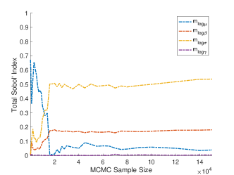
Fig. 5 illustrates the Sobol’ indices of $F_{\text{mean}}$. The computed indices are compared against benchmark values which are computed by sampling the analytic form of the QoI.

(a) PCE

(b) SW-ELM

(c) First-order Sobol’ indices of $F_{\text{mean}}$

(d) Total Sobol’ indices of $F_{\text{mean}}$

Figure 5: Top left: Convergence experiment for $F_{\text{mean}}$ using PCE surrogate. Top right: Convergence experiment for $F_{\text{mean}}$ using SW-ELM surrogate. Bottom left: Comparison of true first-order Sobol’ indices and surrogate-estimated indices where $F_{\text{mean}}$ evaluations approximated with $M=9^{4}$ MCMC samples. Bottom right: Comparison of true total Sobol’ indices and surrogate-estimated indices where $F_{\text{mean}}$ evaluations approximated with $M=9^{4}$ MCMC samples.

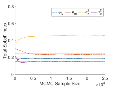
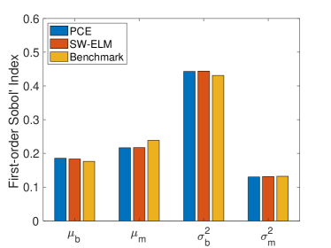
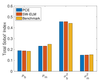
Note that With only a modest number of about 1000 MCMC samples, we can ascertain the correct importance ranking of the total Sobol’ indices of $F_{\text{mean}}$. By 5000 samples, the total Sobol’ indices have converged. Also, as before, the two surrogate modeling approaches provide similar results.

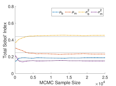
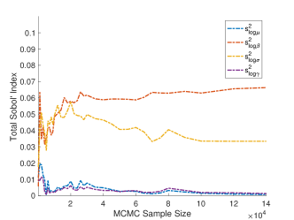
In Fig. 6, we consider $F_{\text{var}}$.

(a) PCE

(b) SW-ELM

(c) First-order Sobol’ indices of $F_{\text{var}}$

(d) Total Sobol’ indices of $F_{\text{var}}$

Figure 6: Top left: Convergence experiment for $F_{\text{var}}$ using PCE surrogate. Top right: Convergence experiment for $F_{\text{var}}$ using SW-ELM surrogate. Bottom left: Comparison of true first-order Sobol’ indices and surrogate-estimated indices where $F_{\text{var}}$ evaluations approximated with $M=9^{4}$ MCMC samples. Bottom right: Comparison of true total Sobol’ indices and surrogate-estimated indices where $F_{\text{var}}$ evaluations approximated with $M=9^{4}$ MCMC samples.

We note that the Sobol’ indices for the $F_{\text{var}}$ take longer to converge than for $F_{\text{mean}}$, for the present QoI. However, even with a modest number of MCMC samples (about 2500), the Sobol’ indices provide the correct ranking of importance. The total indices converge with around $10^{4}$ MCMC samples.

The numerical studies for the present model linear inverse problem provide a proof-of-concept study of Algorithm 1. In particular, availability of analytic expressions for the HS mappings enables testing the accuracy of the computed results. We note that a modest MCMC sample size is sufficient to obtain the correct parameter rankings. We also observe that fewer MCMC samples are required to estimate the indices $F_{\text{mean}}$ compared to $F_{\text{var}}$. This is not surprising, because computing second order moments typically require more effort than that required for computing the mean.

5.2 Nonlinear Bayesian inverse problem based on SEIR model

In this section, we consider a Bayesian inverse problem governed by the susceptible-exposed-infected-recovered (SEIR) model [51, 52] epidemic model. In Section 5.2.1 we discuss the governing SEIR model and the Bayesian inverse problem under study. In Section 5.2.2, we study the proposed importance sampling procedure for computing the HS mappings under study. Finally, in Section 5.2.3, we present our computational results for GSA of the present Bayesian inverse problem with respect to prior hyperparameters.

5.2.1 The inverse problem

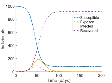
The SEIR model simulates the time dynamics of an epidemic outbreak in a population. The model has four compartments, $S$, $E$, $I$, and $R$, corresponding to the susceptible, exposed, infected, and recovered populations. The individuals in the exposed compartment are those who have been exposed to the disease but are not yet displaying signs of infection. The individuals in the $I$ compartment are infected and infectious. We consider a standard SEIR model where we assume recovered individuals cannot be reinfected. Additionally, we assume that the natural birth and death rates are equal and neglect disease related mortality. This ensures that the total population $N=S+E+I+R$ remains constant over time. The present model is described by the following system of nonlinear ordinary differential equations (ODEs):

$$\dot{S} =\mu N-\beta SI/N-\mu S,$$ (27)

$$\dot{E} =\beta SI/N-(\sigma+\mu)E,$$

$$\dot{I} =\sigma E-(\gamma+\mu)I,$$

$$\dot{R} =\gamma I-\mu R.$$

There are four model parameters in the above system which we seek to estimate. The infection rate $\beta$, in units days^-1, represents how quickly an infected individual infects a susceptible individual. The recovery rate $\gamma$, in units days^-1, represents how fast an infected individual recovers from infection. The latency rate $\sigma$, in units days^-1, represents how long it takes for an exposed individual to display symptoms. Lastly, there is also a parameter $\mu$, with units individuals per day, which represents both the natural birth rate and the natural death rate. In the model, individuals are only born susceptible while individuals in any compartment can die a natural death. As noted before, since the birth and death rates are the same, the total population size remains constant.

Setup. For the purposes of this example, we simulate an epidemic governed by the SEIR model for a population of $N=1000$ individuals. The nominal parameters and initial conditions are detailed in Table 1. The nominal parameter values will be used as “ground-truth” in the computational studies that follow.

Model Parameter	Value	Initial Condition	Value
$\mu$	$5.48\times 10^{-5}$	$S_{0}$	$999$
$\beta$	$1/2.5$	$E(0)$	$0$
$\sigma$	$1/3$	$I(0)$	$1$
$\gamma$	$1/7$	$R(0)$	$0$

Table 1: Model parameters and initial conditions used to simulate the SEIR model (27) in Fig. 7.

The dynamics of the epidemic under these conditions are shown in Fig. 7 (left).

Figure 7: Left: Simulated dynamics of an epidemic outbreak following the SEIR model. The total population is $N=1000$ individuals and the model parameters are $\mu=5.48\times 10^{-5}$ individuals$/$day, $\beta=1/2.5$ days^-1, $\sigma=1/3$ days^-1, and $\gamma=1/7$ days^-1. Initially, there is one infected individuals and there are no exposed individuals. Right: Simulated data of the epidemic outbreak compared to the true infected dynamics. The simulated infected data is taken by adding noise to values from the true model. The noise is sampled from the normal distribution $\mathcal{N}(0,30^{2})$.

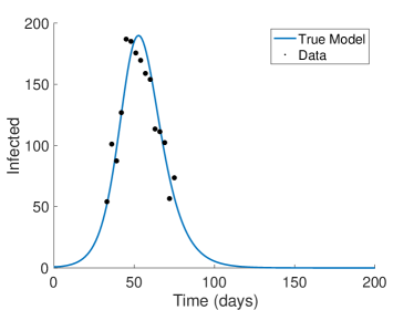
Next, we formulate a Bayesian inverse problem. In what follows, we formulate the inverse problem as that of estimating the log of the uncertain model parameters. Hence, we consider the inversion parameter vector, ${\mathchoice{\mbox{\boldmath$\displaystyle{\theta}$}}{\mbox{\boldmath$\textstyle{\theta}$}}{\mbox{\boldmath$\scriptstyle{\theta}$}}{\mbox{\boldmath$\scriptscriptstyle{\theta}$}}}=\big{[}\begin{array}[]{cccc}\log\mu&\log\beta&\log\sigma&\log\gamma\end{array}\big{]}^{\top}$. The data measurements, used to solve the inverse problem, consist of simulated data $\{(t_{k},I_{k})\}$ at times $t_{k}=3k+30,$ where $k=1,\ldots,15$. These simulated data measurements are obtained by solving the SEIR model with ground-truth parameter values and adding random noise. The noise at each measurement is identically independently distributed from a normal distribution $\mathcal{N}(0,30^{2})$. The simulated data compared to the true model are shown in Fig. 7 (right).

We use a Gaussian prior $\mathcal{N}({\mathchoice{\mbox{\boldmath$\displaystyle{m}$}}{\mbox{\boldmath$\textstyle{m}$}}{\mbox{\boldmath$\scriptstyle{m}$}}{\mbox{\boldmath$\scriptscriptstyle{m}$}}}_{\text{pr}},{\mathchoice{\mbox{\boldmath$\displaystyle{\Sigma}$}}{\mbox{\boldmath$\textstyle{\Sigma}$}}{\mbox{\boldmath$\scriptstyle{\Sigma}$}}{\mbox{\boldmath$\scriptscriptstyle{\Sigma}$}}}_{\text{pr}})$ on the inversion parameter vector $\boldsymbol{\theta}$ with

$${\mathchoice{\mbox{\boldmath$\displaystyle{m}$}}{\mbox{\boldmath$\textstyle{m}$}}{\mbox{\boldmath$\scriptstyle{m}$}}{\mbox{\boldmath$\scriptscriptstyle{m}$}}}_{\text{pr}}=\left[\begin{array}[]{c}m_{\log\mu}\\ m_{\log\beta}\\ m_{\log\sigma}\\ m_{\log\gamma}\end{array}\right],\quad{\mathchoice{\mbox{\boldmath$\displaystyle{\Sigma}$}}{\mbox{\boldmath$\textstyle{\Sigma}$}}{\mbox{\boldmath$\scriptstyle{\Sigma}$}}{\mbox{\boldmath$\scriptscriptstyle{\Sigma}$}}}_{\text{pr}}=\left[\begin{array}[]{cccc}s_{\log\mu}^{2}&0&0&0\\ 0&s_{\log\beta}^{2}&0&0\\ 0&0&s_{\log\sigma}^{2}&0\\ 0&0&0&s_{\log\gamma}^{2}\end{array}\right].$$ (28)

Note that, unlike the inverse problem in Section 5.1, this Bayesian inverse problem is nonlinear. In this case, we do not have access to an analytically known posterior distribution. This means Markov Chain Monte Carlo (MCMC) is needed to sample from the posterior distribution.

Uncertainty in prior hyperparameters. We assume there is uncertainty in the hyperparameters that appear in (28). Specifically, we consider the vector

$${\mathchoice{\mbox{\boldmath$\displaystyle{\xi}$}}{\mbox{\boldmath$\textstyle{\xi}$}}{\mbox{\boldmath$\scriptstyle{\xi}$}}{\mbox{\boldmath$\scriptscriptstyle{\xi}$}}}=\big{[}\begin{array}[]{cccccccc}m_{\log\mu}&m_{\log\beta}&m_{\log\sigma}&m_{\log\gamma}&s_{\log\mu}^{2}&s_{\log\beta}^{2}&s_{\log\sigma}^{2}&s_{\log\gamma}^{2}\end{array}\big{]}^{\top}$$

of parameters that define the prior as uncertain. In the present study, we assume that the entries of $\textstyle{\xi}$ are independent uniformly distributed random variables, as specified in Table 2.

Mean Hyperparameter	Distribution	Variance Hyperparameter	Distribution
$m_{\log\mu}$	$\mathcal{U}([-15,-5])$	$s_{\log\mu}^{2}$	$\mathcal{U}([0.5,1.5])$
$m_{\log\beta}$	$\mathcal{U}([-2.25,-0.75])$	$s_{\log\beta}^{2}$	$\mathcal{U}([0.5,1.5])$
$m_{\log\sigma}$	$\mathcal{U}([-2.25,-0.75])$	$s_{\log\sigma}^{2}$	$\mathcal{U}([0.5,1.5])$
$m_{\log\gamma}$	$\mathcal{U}([-2.25,-0.75])$	$s_{\log\gamma}^{2}$	$\mathcal{U}([0.5,1.5])$

Table 2: Intervals for admissible hyperparameter values of the prior $\boldsymbol{\theta}\sim\mathcal{N}({\mathchoice{\mbox{\boldmath$\displaystyle{m}$}}{\mbox{\boldmath$\textstyle{m}$}}{\mbox{\boldmath$\scriptstyle{m}$}}{\mbox{\boldmath$\scriptscriptstyle{m}$}}}_{\text{pr}},{\mathchoice{\mbox{\boldmath$\displaystyle{\Sigma}$}}{\mbox{\boldmath$\textstyle{\Sigma}$}}{\mbox{\boldmath$\scriptstyle{\Sigma}$}}{\mbox{\boldmath$\scriptscriptstyle{\Sigma}$}}}_{\text{pr}})$. Each hyperparameter is uniformly distributed on an interval perturbed $\pm 50\%$ of the respective nominal value.

Quantity of interest. An important quantity of interest in epidemiology is the basic reproduction number, denoted $R_{0}$. It can be interpreted as the number of secondary infections caused, on average, by a single individual [51]. Determining $R_{0}$ of an epidemic is key to understanding how severe the outbreak could be. For the SEIR model 27, $R_{0}$ takes the form

$$R_{0}=\frac{\beta}{\gamma+\mu}\frac{\sigma}{\sigma+\mu}.$$ (29)

For the epidemic in Fig. 7, $R_{0}=2.7985$. The importance of $R_{0}$ makes it a prime area to apply uncertainty quantification and robustness analysis. In [55], the robustness of $R_{0}$ estimates to model parameters is considered through local derivative-based methods. Hence, we focus on $R_{0}$ as the QoI,

$$q({\mathchoice{\mbox{\boldmath$\displaystyle{\theta}$}}{\mbox{\boldmath$\textstyle{\theta}$}}{\mbox{\boldmath$\scriptstyle{\theta}$}}{\mbox{\boldmath$\scriptscriptstyle{\theta}$}}})=\frac{e^{\theta_{2}}}{e^{\theta_{4}}+e^{\theta_{1}}}\frac{e^{\theta_{3}}}{e^{\theta_{3}}+e^{\theta_{1}}}.$$

5.2.2 Parameter estimation and importance sampling

Before we can implement Algorithm 1, we have to choose the importance sampling distribution. In accordance with the discussion in Section 4, we choose the importance sampling distribution $\pi_{\text{pr}}^{\text{IS}}$ as $\mathcal{N}({\mathchoice{\mbox{\boldmath$\displaystyle{m}$}}{\mbox{\boldmath$\textstyle{m}$}}{\mbox{\boldmath$\scriptstyle{m}$}}{\mbox{\boldmath$\scriptscriptstyle{m}$}}}_{\text{pr}}^{\text{IS}},{\mathchoice{\mbox{\boldmath$\displaystyle{\Sigma}$}}{\mbox{\boldmath$\textstyle{\Sigma}$}}{\mbox{\boldmath$\scriptstyle{\Sigma}$}}{\mbox{\boldmath$\scriptscriptstyle{\Sigma}$}}}_{\text{pr}}^{\text{IS}})$ with

$${\mathchoice{\mbox{\boldmath$\displaystyle{m}$}}{\mbox{\boldmath$\textstyle{m}$}}{\mbox{\boldmath$\scriptstyle{m}$}}{\mbox{\boldmath$\scriptscriptstyle{m}$}}}_{\text{pr}}^{\text{IS}}=\left[\begin{array}[]{cc}-10\\ -1.5\\ -1.5\\ -1.5\end{array}\right],\quad\boldsymbol{\Sigma}_{\text{pr}}^{\text{IS}}=\left[\begin{array}[]{cccc}3^{2}&0&0&0\\ 0&2^{2}&0&0\\ 0&0&2^{2}&0\\ 0&0&0&2^{2}\end{array}\right].$$ (30)

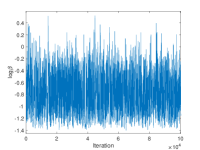
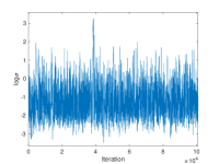
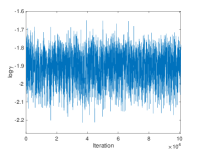
Because $m_{\log\mu}$ takes a wider range of values compared to the other means, we impose a large variance on $\log\mu$ in $\pi_{\text{pr}}^{\text{IS}}$. We construct the corresponding posterior $\pi_{\text{post}}^{\text{IS}}$ using the DRAM algorithm. The first $10^{3}$ samples are removed for burn-in. After sufficient burn-in, we generate $1.5\times 10^{5}$ from the posterior. We present the MCMC chains of log parameters and their respective marginal posterior distributions in Fig. 8.

Figure 8: Results of Bayesian parameter estimation for SEIR example. Chains are constructed by taking $1.5\times 10^{5}$ samples after $10^{3}$ iterations of burn-in. Marginal distributions are constructed by kernel density estimation on the respective MCMC chains.

In Fig. 9 (left), we evaluate the effectiveness of our importance sampling distribution by examining the distribution of effective sample sizes. We also compare the distribution of $R_{0}$ values, with respect to $\pi_{\text{post}}^{\text{IS}}$, compared to the posterior distributions for three realizations of the prior hyperparameters in Fig. 9 (right).

Figure 9: Left: Distribution of effective sample sizes using $\pi_{\text{post}}^{\text{IS}}$. Right: Kernel density estimates of the distribution for $\pi_{\text{post}}^{\text{IS}}$ compared to those for selected target posterior distributions.

These results indicate that we can use $\pi_{\text{post}}^{\text{IS}}$ as an importance sampling distribution for the target posteriors.

5.2.3 Sensitivity analysis

Here, we study the sensitivity of the HS mappings $F_{\text{mean}}$, $F_{\text{var}}$, and $F_{\text{MAP}}$ to prior hyperparameters, relative to the QoI $q({\mathchoice{\mbox{\boldmath$\displaystyle{\theta}$}}{\mbox{\boldmath$\textstyle{\theta}$}}{\mbox{\boldmath$\scriptstyle{\theta}$}}{\mbox{\boldmath$\scriptscriptstyle{\theta}$}}})=R_{0}$. As discussed in Section 4, $F_{\text{MAP}}$ is not evaluated the same way as the other two HS mappings—it is evaluated by solving an optimization problem. Therefore, we only include convergence studies for $F_{\text{mean}}$ and $F_{\text{var}}$.

For each HS mapping, surrogate models are constructed using $10^{3}$ realizations of $\textstyle{\xi}$, drawn using Latin hypercube sampling (LHS). For polynomial chaos expansion surrogates, we use expansions of total degree 6. SW-ELM surrogates use $800$ realizations for training and $200$ for validation during the weight sparsification step.

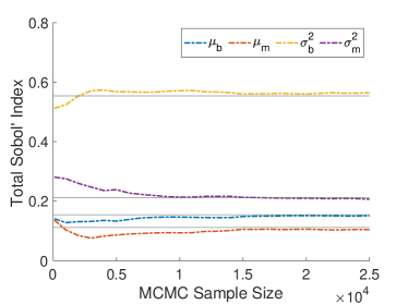
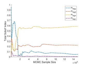
We start by studying the total Sobol’ indices for $F_{\mathrm{var}}$ and $F_{\mathrm{mean}}$. We track the convergence of these indices as we increase the number of MCMC samples taken from $\pi_{\text{post}}^{\text{IS}}$ to up to $1.5\times 10^{5}$ samples. The results are reported in Fig. 10.

(a) SW-ELM

(b) SW-ELM

(c) PCE

(d) PCE

Figure 10: Convergence of the total indices of $F_{\mathrm{mean}}(\boldsymbol{\xi})$ with increasing MCMC sample size, comparing SW-ELM and PCE results. Total indices of the mean hyperparameters and variance hyperparameters are displayed separately.

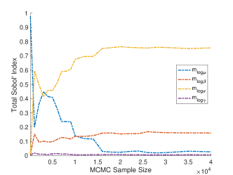
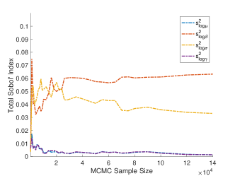
We observe that the estimators for the larger Sobol’ indices converge faster. However, our importance ranking remains constant after $4\times 10^{4}$ MCMC samples. The convergence of the total indices of $F_{\mathrm{var}}$ are studied in Fig. 11.

(a) SW-ELM

(b) SW-ELM

(c) PCE

(d) PCE

Figure 11: Convergence of the total indices of $F_{\mathrm{var}}(\boldsymbol{\xi})$ with increasing MCMC sample size, comparing SW-ELM and PCE results. Total indices of the mean hyperparameters and variance hyperparameters are displayed separately.

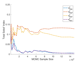
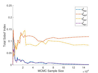
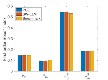
As was observed when studying the linear Bayesian inverse problem, evaluating the variance accurately requires more MCMC samples compared to evaluating the mean. Finally, we compare the converged total Sobol’ indices of $F_{\mathrm{mean}}(\boldsymbol{\xi}),F_{\mathrm{var}}(\boldsymbol{\xi})$ with those of $F_{\mathrm{MAP}}(\boldsymbol{\xi})$ in Fig. 12.

(a) Total Sobol’ indices of $F_{\text{mean}}$

(b) Total Sobol’ indices of $F_{\text{var}}$

(c) Total Sobol’ indices of $F_{\text{MAP}}$

Figure 12: Comparison of total Sobol’ indices of $F_{\text{mean}}$, $F_{\text{var}}$, and $F_{\text{MAP}}$ estimated by SW-ELM and PCE surrogate-assisted GSA. $F_{\text{mean}}$ and $F_{\text{var}}$ are evaluated using $1.5\times 10^{5}$ MCMC samples drawn from $\pi_{\text{post}}^{\text{IS}}$.

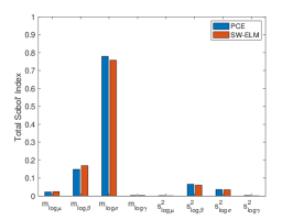
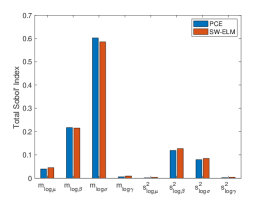
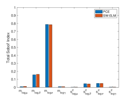
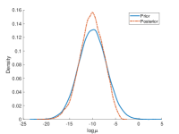
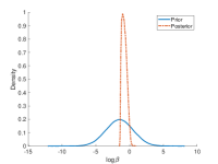
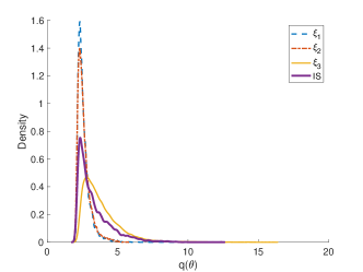
Overall, we note that the results from the SW-ELM and sparse regression PCE results agree. The indicates that the present computations are stable with respect to the choice of the surrogate model. The global sensitivity analysis of the posterior mean, variance, and MAP point in Fig. 12 allow us to infer much information about which hyperparameters in the prior matter and which do not. The Sobol’ indices suggest that the uncertainty in the prior mean of $\log\gamma$ and prior variances of $\log\mu,\log\gamma$ can be ignored. To illustrate this, we compare the distributions of $F_{\mathrm{mean}},F_{\mathrm{var}}$, and $F_{\mathrm{MAP}}$ before and after these prior hyperparameters are fixed at their nominal values in Fig. 13.

(a) Mean

(b) Variance

(c) MAP Point

Figure 13: Kernel density estimates of $F(\boldsymbol{\xi})$ when sampled over all prior hyperparameters compared to when the prior mean of $\log\gamma$ and prior variances of $\log\mu,\log\gamma$ are fixed at the nominal values of -1.5, 1, and 1, respectively. These estimates on superimposed on one another for $F_{\mathrm{mean}}(\boldsymbol{\xi})$ (left), $F_{\mathrm{var}}(\boldsymbol{\xi})$ (right), and $F_{\mathrm{MAP}}(\boldsymbol{\xi})$ (bottom).

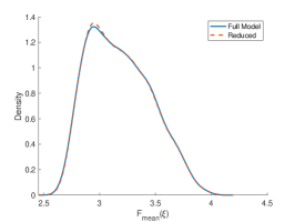
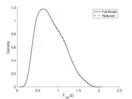
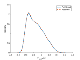
The density estimates in Fig. 13 confirm that those three prior hyperparameters have little influence over the posterior mean, variance, and MAP point. Thus, the experimental resources should be put towards finding more knowledge about the other hyperparameters.

6 Conclusion

We have developed a computational approach for global sensitivity analysis of Bayesian inverse problems with respect to hyperparameters defining the prior. Our results indicate that the posterior distribution can exhibit complex dependence on such hyperparameters. Consequently, the uncertainty in the prior hyperparameters lead to uncertainty in posterior statistics of the prediction/goal quantities of interest which needs to be accounted for. The results of GSA provide valuable insight this context. Such an analysis reveals the prior hyperparameters that are most influential to the posterior statistics of prediction quantities of interest and whose specification requires care. Our computational studies provide a proof-of-concept of the proposed approach and indicate its viability. In particular, at the cost of one MCMC run, we can obtain reliable estimates of the sensitivity of moment-based hyperparameter-to-statistic mappings with respect to prior hyperparameters.

An important aspect of our approach is the proposed importance sampling procedure. A limitation of the present study is that the importance sampling prior in (12) was chosen in an empirical manner. While this can be practical in many cases, developing a systematic approach for picking this distribution is an interesting and important avenue of future investigations. This can be facilitated, e.g., by considering an appropriate optimization problem for finding $\pi_{\text{pr}}^{\text{IS}}$. This requires definition of suitable performance objectives for $\pi_{\text{pr}}^{\text{IS}}$ that are tractable to optimize.

A related line of inquiry is exploration of techniques such as variational inference [56] or the Laplace approximation [57] to the posterior for obtaining an importance sampling posterior $\pi_{\text{post}}^{\text{IS}}$. This is necessary for computationally intensive inverse problems where even one MCMC run might be prohibitive. Yet another direction for future work is the development of hyperparameter screening steps. A tried-and-true approach is to screen via derivative-based global sensitivity measures [58, 59], after which a variance-based analysis may be conducted. This would be important for inverse problems with a large number of prior hyperparameters.

References

- [1] J. A. Scales, L. Tenorio, Prior information and uncertainty in inverse problems, Geophysics 66 (2) (2001) 389–397.
- [2] J. O. Berger, Robust Bayesian analysis: sensitivity to the prior, Journal of Statistical Planning and Inference 25 (3) (1990) 303–328.
- [3] J. O. Berger, E. Moreno, L. Pericchi, M. Bayarri, J. Bernardo, J. Cano, J. Horra, J. Martín, D. Rios, B. Betrò, A. Dasgupta, P. Gustafson, L. Wasserman, J. Kadane, C. Srinivasan, M. Lavine, A. O’Hagan, W. Polasek, C. Robert, S. Sivaganesan, An overview of robust Bayesian analysis, Test 3 (1994) 5–124.
- [4] S. D. Hill, J. C. Spall, Sensitivity of a Bayesian Analysis to the Prior Distribution, IEEE Transactions on Systems, Man, and Cybernetics: Systems 24 (1994) 216–221.
- [5] J. O. Berger, D. R. Insua, F. Ruggeri, Bayesian Robustness, in: D. R. Insua, F. Ruggeri (Eds.), Robust Bayesian Analysis, Springer, 2000, pp. 1–32.
- [6] H. Lopes, J. Tobias, Confronting Prior Convictions: On Issues of Prior Sensitivity and Likelihood Robustness in Bayesian Analysis, Annual Review of Economics 3 (2011) 107–131.
- [7] H. Owhadi, C. Scovel, T. Sullivan, On the Brittleness of Bayesian Inference, SIAM Review 57 (4) (2015) 566–582.
- [8] J. Watson, C. Holmes, Approximate Models and Robust Decisions, Statistical Science 31 (4) (2016) 465–489.
- [9] R. Giordano, T. Broderick, M. I. Jordan, Covariances, Robustness, and Variational Bayes, Journal of Machine Learning Research 19 (2018) 1–58.
- [10] A. Gelman, J. B. Carlin, H. S. Stern, D. B. Dunson, A. Vehtari, D. B. Rubin, Models for robust inference, in: Bayesian Data Analysis, Chapman and Hall/CRC, 2013, Ch. 17, pp. 435–447.
- [11] R. van de Schoot, S. Depaoli, R. King, B. Kramer, K. Märtens, M. G. Tadesse, M. Vannucci, A. Gelman, D. Veen, J. Willemsen, C. Yau, Bayesian statistics and modelling, Nature Reviews Methods Primers 1 (1) (2021) 1–26.
- [12] I. Sunseri, A. Alexanderian, J. Hart, B. van Bloemen Waanders, Hyper-differential sensitivity analysis for nonlinear Bayesian inverse problems, preprint (2022).
- [13] W. M. Reese, J. Hart, B. van Bloemen Waanders, M. Perego, J. Jakeman, A. Saibaba, Hyper-differential sensitivity analysis in the context of Bayesian inference applied to ice-sheet problems (2022).
- [14] A. Chowdhary, A. Alexanderian, S. Tong, G. Stadler, Sensitivity Analysis of the Information Gain in Infinite-Dimensional Bayesian Linear Inverse Problems, preprint (2023).
- [15] J. Hart, B. van Bloemen Waanders, R. Herzog, Hyper-Differential Sensitivity Analysis of Uncertain Parameters in PDE-Constrained Optimization, International Journal for Uncertainty Quantification 10 (3) (2020) 225–248.
- [16] I. Sunseri, J. Hart, B. van Bloemen Waanders, A. Alexanderian, Hyper-differential sensitivity analysis for inverse problems constrained by partial differential equations, Inverse Problems 36 (12) (2020) 125001.
- [17] I. Vernon, J. P. Gosling, A Bayesian Computer Model Analysis of Robust Bayesian Analyses, Bayesian Analysis (2022) 1–33.
- [18] C. J. Geyer, E. A. Thompson, Constrained Monte Carlo Maximum Likelihood for Dependent Data, Journal of the Royal Statistical Society. Series B (Methodological) 54 (3) (1992) 657–699.
- [19] N. Madras, M. Piccioni, Importance Sampling for Families of Distributions, The Annals of Applied Probability 9 (4) (1999) 1202–1225.
- [20] C. J. Geyer, E. A. Thompson, Annealing Markov Chain Monte Carlo with Applications to Ancestral Inference, Journal of the American Statistical Association 90 (431) (1995) 909–920.
- [21] C. J. Geyer, Importance Sampling, Simulated Tempering, and Umbrella Sampling, in: S. Brooks, A. Gelman, G. Jones, X.-L. Meng (Eds.), Handbook of Markov Chain Monte Carlo, Chapman and Hall/CRC, 2011, Ch. 11, pp. 295–311.
- [22] A. B. Owen, Importance sampling, in: Monte Carlo theory, methods and examples, 2013, Ch. 9.
- [23] M. Merritt, A. Alexanderian, P. A. Gremaud, Global Sensitivity Analysis of Rare Event Probabilities Using Sublet Simulation and Polynomial Chaos Expansions, International Journal for Uncertainty Quantification 13 (1) (2023) 53–67.
- [24] A. Tarantola, Inverse Problem Theory and Methods for Model Parameter Estimation, Society for Industrial and Applied Mathematics.
- [25] A. Saltelli, I. Sobol’, Sensitivity analysis for nonlinear mathematical models: numerical experience, Matematicheskoe Modelirovanie 7 (11) (1995) 16–28.
- [26] I. Sobol’, Global sensitivity indices for nonlinear mathematical models and their Monte Carlo estimates, Mathematics and Computers in Simulation 55 (1–3) (2001) 271–280.
- [27] A. Saltelli, M. Ratto, T. Andres, F. Campolongo, J. Cariboni, D. Gatelli, M. Saisana, S. Tarantola, Global sensitivity analysis: the primer, John Wiley & Sons, 2008.
- [28] R. C. Smith, Uncertainty quantification: Theory, implementation, and applications, Society for Industrial and Applied Mathematics, 2014.
- [29] B. Iooss, P. Lemaître, A Review on Global Sensitivity Analysis Methods, in: G. Dellino, C. Meloni (Eds.), Uncertainty Management in Simulation-Optimization of Complex Systems: Algorithms and Applications, Springer, 2015, pp. 101–122.
- [30] C. Prieur, S. Tarantola, Variance-based sensitivity analysis: Theory and estimation algorithms, in: R. Ghanem, D. Higdon, H. Owhadi (Eds.), Handbook of Uncertainty Quantification, Springer, 2017, pp. 1217–1239.
- [31] A. Saltelli, P. Annoni, I. Azzini, F. Campolongo, M. Ratto, S. Tarantola, Variance based sensitivity analysis of model output. Design and estimator for the total sensitivity index, Computer Physics Communications 181 (2) (2010) 259–270.
- [32] K. Sargsyan, Surrogate models for uncertainty propagation and sensitivity analysis, in: R. Ghanem, D. Higdon, H. Owhadi (Eds.), Handbook of Uncertainty Quantification, Springer, 2017, pp. 673–698.
- [33] L. Le Gratiet, S. Marelli, B. Sudret, Metamodel-based sensitivity analysis: polynomial chaos expansions and Gaussian processes, in: R. Ghanem, D. Higdon, H. Owhadi (Eds.), Handbook of Uncertainty Quantification, Springer, 2017, pp. 1289–1326.
- [34] B. Sudret, Global sensitivity analysis using polynomial chaos expansions, Reliability Engineering & System Safety 93 (7) (2008) 964–979.
- [35] T. Crestaux, O. Le Maître, J.-M. Martinez, Polynomial chaos expansion for sensitivity analysis, Reliability Engineering & System Safety 94 (7) (2009) 1161–1172.
- [36] O. P. Le Maître, O. M. Knio, Spectral methods for uncertainty quantification, Springer, 2010, with applications to computational fluid dynamics.
- [37] G. Blatman, B. Sudret, Efficient computation of global sensitivity indices using sparse polynomial chaos expansions, Reliability Engineering & System Safety 95 (11) (2010) 1216–1229.
- [38] G. Blatman, B. Sudret, Adaptive sparse polynomial chaos expansion based on least angle regression, Journal of Computational Physics 230 (6) (2011) 2345–2367.
- [39] J. Hampton, A. Doostan, Compressive Sampling Methods for Sparse Polynomial Chaos Expansions, in: R. Ghanem, D. Higdon, H. Owhadi (Eds.), Handbook of Uncertainty Quantification, Springer, 2017, pp. 827–855.
- [40] N. Fajraoui, S. Marelli, B. Sudret, Sequential Design of Experiment for Sparse Polynomial Chaos Expansions, SIAM/ASA Journal on Uncertainty Quantification 5 (1) (2017) 1061–1085.
- [41] E. van den Berg, M. P. Friedlander, Probing the Pareto frontier for basis pursuit solutions, SIAM Journal on Scientific Computing 31 (2) (2008) 890–912.
- [42] E. van den Berg, M. P. Friedlander, SPGL1: A solver for large-scale sparse reconstruction, https://friedlander.io/spgl1 (2019).
- [43] G.-B. Huang, Q.-Y. Zhu, C.-K. Siew, Extreme learning machine: Theory and applications, Neurocomputing 70 (1) (2006) 489–501.
- [44] G.-B. Huang, D. Wang, Y. Lan, Extreme learning machines: a survey, International Journal of Machine Learning and Cybernetics 2 (2) (2011) 107–122.
- [45] J. E. Darges, A. Alexanderian, P. A. Gremaud, Extreme learning machines for variance-based global sensitivity analysis, preprint (2023).
- [46] S. Tokdar, R. Kass, Importance sampling: A review, Wiley Interdisciplinary Reviews: Computational Statistics 2 (2010) 54–60.
- [47] M. D. McKay, R. J. Beckman, W. J. Conover, A Comparison of Three Methods for Selecting Values of Input Variables in the Analysis of Output from a Computer Code, Technometrics 21 (2) (1979) 239–245.
- [48] F. A. Viana, A tutorial on Latin hypercube design of experiments, Quality and Reliability Engineering International 32 (5) (2016) 1975–1985.
- [49] H. Haario, M. Laine, A. Mira, E. Saksman, DRAM: Efficient adaptive MCMC, Statistics and Computing 16 (4) (2006) 339–354.
- [50] M. Laine, Adaptive MCMC Methods With Applications in Environmental and Geophysical Model, Finnish Meteorological Institute Contributions 69 (2008).
- [51] H. W. Hethcote, The Mathematics of Infectious Diseases, SIAM Review 42 (4) (2000) 599–653.
- [52] M. P. Fox, E. W. Gower, Infectious Disease Epidemiology, in: T. L. Lash, T. J. VanderWeele, S. Haneuese, K. J. Rothman (Eds.), Modern Epidemiology, Lippincott Williams & Wilkin, 2021, Ch. 32, pp. 1175–1232.
- [53] K. B. Petersen, M. S. Pedersen, The Matrix Cookbook, http://www2.compute.dtu.dk/pubdb/pubs/3274-full.html, Version 20121115 (2012).
- [54] A. Alexanderian, On the mean and variance of quadratic functionals of Gaussian random vectors, https://aalexan3.math.ncsu.edu/articles/moments_quad.pdf, Technical Note (2021).
- [55] A. Lloyd, Sensitivity of Model-Based Epidemiological Parameter Estimation to Model Assumptions, in: G. Chowell, J. M. Hyman, L. M. A. Bettencourt, C. Castillo-Chavez (Eds.), Mathematical and Statistical Estimation Approaches in Epidemiology, Springer Netherlands, 2009, pp. 123–141.
- [56] D. M. Blei, A. Kucukelbir, J. D. McAuliffe, Variational Inference: A Review for Statisticians, Journal of the American Statistical Association 112 (518) (2017) 859–877.
- [57] A. Gelman, J. B. Carlin, H. S. Stern, D. B. Dunson, A. Vehtari, D. B. Rubin, Modal and distributional approximations, in: Bayesian Data Analysis, Chapman and Hall/CRC, 2013, Ch. 13, pp. 311–350.
- [58] I. Sobol’, S. Kucherenko, Derivative based global sensitivity measures and their link with global sensitivity indices, Mathematics and Computers in Simulation 79 (10) (2009) 3009–3017.
- [59] S. Kucherenko, B. Iooss, Derivative based global sensitivity measures, in: R. Ghanem, D. Higdon, H. Owhadi (Eds.), Handbook of Uncertainty Quantification, Springer, 2017, pp. 1241–1263.