Structure preserving numerical methods for the ideal compressible MHD system

Abstract

We introduce a novel structure-preserving method in order to approximate the compressible ideal Magnetohydrodynamics (MHD) equations. This technique addresses the MHD equations using a non-divergence formulation, where the contributions of the magnetic field to the momentum and total mechanical energy are treated as source terms. Our approach uses the Marchuk-Strang splitting technique and involves three distinct components: a compressible Euler solver, a source-system solver, and an update procedure for the total mechanical energy. The scheme allows for significant freedom on the choice of Euler’s equation solver, while the magnetic field is discretized using a curl-conforming finite element space, yielding exact preservation of the involution constraints. We prove that the method preserves invariant domain properties, including positivity of density, positivity of internal energy, and the minimum principle of the specific entropy. If the scheme used to solve Euler’s equation conserves total energy, then the resulting MHD scheme can be proven to preserve total energy. Similarly, if the scheme used to solve Euler’s equation is entropy-stable, then the resulting MHD scheme is entropy stable as well. In our approach, the CFL condition does not depend on magnetosonic wave-speeds, but only on the usual maximum wavespeed from Euler’s system. To validate the effectiveness of our method, we solve a variety of ideal MHD problems, showing that the method is capable of delivering high-order accuracy in space for smooth problems, while also offering unconditional robustness in the shock hydrodynamics regime as well.

1 Introduction

Magnetohydrodynamic (MHD) equations model the dynamics of plasma, which is an ionizied gas at high temperatures. The ideal MHD equations combines: the fluid dynamics equations description of Euler equations, with zero-permittivity limit of Maxwell’s equations and Ohm’s law closure. The model considers both the movement of the conductive fluid and its interaction with magnetic fields. The MHD equations are widely used in astrophysics applications as well as in nuclear fusion research, where it is used to study and control instabilities in the plasma confinement.

Solutions to the MHD system contain contact, shock, and rarefaction waves. In addition, the interaction of fluid and magnetic fields at very high temperatures pose additional challenges for MHD simulations. Despite these difficulties, numerical solutions of the MHD system are vital to predict phenomena in various scientific fields such as plasma physics and astrophysics. Furthermore, when performing numerical simulations of the MHD system, it is crucial to ensure the preservation of essential structure of the solution, such as positivity properties, conservation of total energy, and involution constraints.

Various schemes that retain several of these properties, in particular for the compressible Euler equations, are published in existing literature. For instance, the works of [32, 42, 14], along with references provided therein, represent just a subset of the comprehensive research dedicated to achieving positivity-preserving approximations for the compressible Euler equations, using finite volume, discontinuous Galerkin, and finite element methods. Unfortunately, direct extension of these methods for the MHD system is not straighforward due to the additional induction equation for the magnetic field and corresponding to the magnetic stress/force. In particular, the standard MHD model in divergence form is only valid if $\text{div}\,\mathbf{}\bm{\mathcal{B}}\equiv 0$ at all times. A slight violation of the divergence-free condition can lead to negative internal energy, which will cause the numerical simulation to fail catastrophically, see e.g., [40, 41]. It should be emphasized that the divergence formulation of the MHD system is valid only for sufficiently smooth solutions. However, in the case of weakly differentiable and discontinuous solutions, $\text{div}\,\mathbf{}\bm{\mathcal{B}}$ cannot be pointwise zero. To the best of our knowledge, none of the divergence cleaning techniques, such as [10], can completely eliminate the discrepancy error of the divergence of $\bm{\mathcal{B}}$.

In this paper, instead of using the MHD equations in divergence form, see (2), which is widely used in scientific works, we proposed to use the induction equation and preserve the magnetic forces acting on the momentum and total mechanical energy as source terms. More precisely, we propose solving

$$\partial_{t}\rho+\text{div}\,\mathbf{}\bm{m} =0\,,$$ (1a)

$$\partial_{t}\bm{m}+\text{div}\,\mathbf{}(\rho^{-1}\bm{m}\bm{m}^{\top}+\mathbb{I}p) =-\mu\bm{\mathcal{H}}\times\text{curl}\,\mathbf{}\bm{\mathcal{H}}\,,$$ (1b)

$$\partial_{t}E+\text{div}\,\mathbf{}\big{(}\tfrac{\bm{m}}{\rho}(E+p)\big{)} =-\mu(\bm{\mathcal{H}}\times\text{curl}\,\mathbf{}\bm{\mathcal{H}})\cdot\tfrac{\bm{m}}{\rho}\,,$$ (1c)

$$\partial_{t}\bm{\mathcal{H}}-\text{curl}\,\mathbf{}(\tfrac{\bm{m}}{\rho}\times\bm{\mathcal{H}}) =0\,,$$ (1d)

where $\rho$ is the density, $\bm{m}$ is the momentum, $E=\frac{1}{2\rho}|\bm{m}|^{2}+\rho e$ is the total mechanical energy, $e$ is the specific internal energy, $\bm{\mathcal{H}}$ is the magnetic field, $p=p(\rho,e)$ is the pressure, $\mathbb{I}\in\mathbb{R}^{d\times d}$ denotes the identity matrix with $d$ being the space dimension, and $\mu>0$ is the magnetic permeability constant. Taking the divergence to both sides of (1d) we obtain the condition $\partial_{t}\text{div}\,\mathbf{}\bm{\mathcal{H}}=0,$ implying that the evolution of the magnetic field $\bm{\mathcal{H}}$ is such that $\text{div}\,\mathbf{}\bm{\mathcal{H}}(t)\equiv\text{div}\,\mathbf{}\bm{\mathcal{H}}_{0}$ for all $t\geq 0$, where $\bm{\mathcal{H}}_{0}$ is the initial data.

Note, that for the case of smooth (e.g., $\mathcal{C}^{1}$-continuous or better) divergence-free solutions the formulation (1) is equivalent to the MHD system in the divergence form (2). However, for the case of weakly-differentiable and discontinuous solutions, we should regard (1) and (2) as entirely different models. In particular, there is no reason to believe that (1) and (2) should produce the same families of discontinuous solutions, see for instance [34, p. 253] on a related discussion. We emphasize that formulation (2) is not valid without the assumption $\text{div}\,\mathbf{}\bm{\mathcal{B}}=\text{div}\,\mathbf{}\bm{\mathcal{B}}_{0}=0$ since it is an intrinsic part of its derivation. On other hand, formulation (1) does not need or use the condition $\text{div}\,\mathbf{}\bm{\mathcal{H}}\equiv 0$: there is no mathematical reason to incorporate such assumption.

From a practical point of view, regardless of whether we prefer source-formulation (1) or divergence formulation (2), any numerical method satisfying the following:

• Preservation of pointwise stability properties: such as pointwise positivity of the density and minimum principle of the specific entropy;

• Preservation of involution constraints, in this case, preservation of the weak-divergence;

• Preservation of total energy;

• Preservation of second order accuracy (or higher) for smooth solutions;

• Preservation of discrete entropy-dissipation properties.

is a desirable method for engineering and scientific applications. List (i)-(v) is quite ambitious and we are not aware of any numerical scheme capable of preserving properties (i)-(v) simultaneously. We highlight that designing a scheme that preserves just one of these properties (e.g., formal high-order accuracy, see for instance [8, 9]) does not pose a major challenge. The mathematical challenge of structure preservation lies in the satisfaction of two or more of these properties simultaneously. In this manuscript, we advocate for the use of formulation (1), instead of the usual divergence form (2), as better fit in order to preserve properties (i)-(v) outlined above.

In [8] it was proved that by adding a viscous term to each equation of the ideal MHD system (i.e., conservation of mass, conservation of momentum, conservation of total energy, and the induction equation) one can achieve positivity of density and internal energy, minimum principle of the specific entropy, and satisfaction of all generalized entropies. In this article we improve the result of [8]. We prove that the viscous regularization of mass, momentum, and total mechanical energy is sufficient to achieve the above mentioned properties (i.e., positivity of density and internal energy, minimum principle of the specific entropy, and compatibility with all generalized entropies). This shows that there is no need to regularize the induction equation. This is a rather puzzling result, hinting at the idea that the inclusion of the $\bm{\mathcal{B}}$ field in the MHD Riemann problem is an artificial construct. We propose to separate the evolution equation of $\bm{\mathcal{B}}$ from the other components of the system (density, momentum, and total mechanical energy), as originally described by the non-divergence formulation (1). This is by no means a new idea: treating $\bm{\mathcal{B}}$ independently using its own spatial discretization has been proposed, for example, in [29, 22, 12] and references therein. However, our approach still represents a major departure from previously existing ideas and methods for the MHD system:

• The induction equation is not treated as an isolated object, but rather as a constituent of a Hamiltonian system consisting in: the balance of momentum subject to the Lorentz force $\mu(\text{curl}\,\mathbf{}\bm{\mathcal{H}}\times\bm{\mathcal{H}})$, coupled to the induction equation (1d), see for instance expressions (19) and (24). By treating a Hamiltonian system as such, this lends itself to natural definitions of stability that we can preserve in the fully-discrete setting.

• We use no advective stabilization in any form or fashion for the induction equation. This is tacitly suggested by the viscous regularization argument indicating that no artificial viscosity is required for the magnetic field $\bm{\mathcal{H}}$. This is also consistent with Hamiltonian systems, such as (24), where the natural notion of stability is preservation of quadratic invariants. We avoid construing the induction equation as an advective system [19, 21], Friedrich’s system [5], or vanishing-viscosity limit (e.g., conservation law).

• We use a primal (no vector potential) curl-conforming framework in order to discretize the magnetic field $\bm{\mathcal{H}}$. This is consistent with the preservation of weak divergence. We do not pursue to preserve a zero strong-divergence, or use a div-conforming framework as suggested for instance in [4, 22]. However, we show that the method can preserve zero weak-divergence to machine accuracy for smooth as well as non-smooth regimes. We use no divergence cleaning.

• Energy of the non-divergence system (1) is defined by a functional that consists in the sum of a linear $+$ quadratic functional, see Section 2.2. This is quite different from the case of the divergence system (2) where energy stability consists in preserving the property $\int_{\Omega}\mathcal{E}(t)\,\mathrm{d}\bm{x}=\int_{\Omega}\mathcal{E}_{0}\,\mathrm{d}\bm{x}$, which is the preservation of a linear functional.

• The resulting scheme preserves properties (i)-(iv) outlined above. This scheme can be used for smooth as well as extreme shock-hydrodynamics regimes. Property (v), entropy stability, can be preserved as well, provided the hyperbolic solver used to discretize Euler’s subsystem is entropy stable. We make no emphasis on property (v) since there the is a very large literature on the matter. The scheme runs at the CFL of Euler’s system, with no time-step size restriction due to magnetosonic waves. There is, in principle, no limit on the formal spatial accuracy of the scheme.

The outline of the paper is as follows: in Section 2 we provide all the necessary background in relationship to the mathematical properties of the MHD and Euler’s system. In Sections 3.1-3.3 we summarize the main properties of the spatial and temporal discretizations that will be used. In Section 3.4 we present the scheme and make precise its mathematical properties. Finally, in Section 4 we present numerical results illustrating the efficiency of the solver is the context of smooth as well as non-smooth test problems. We highlight that the main ideas advanced in this paper can be implemented using quite general hyperbolic solvers for Euler’s equation. In Section 3.4 we outline the structure and mathematical properties expected from such hyperbolic solver. For the sake of completeness we also describe the hyperbolic solvers used for all computations in A.

2 Main properties of the MHD system

2.1 Vanishing-viscosity limits and invariant sets

In this section we improve the result of [8]. Let us consider the case where initial magnetic field is divergence-free, i.e., $\text{div}\,\mathbf{}\bm{\mathcal{B}}_{0}=0$. As already mentioned in the introduction, this implies that $\text{div}\,\mathbf{}\bm{\mathcal{B}}=0$ also for all time $t$. Therefore, the system (1) can be re-written in the following divergence form:

$$\partial_{t}\rho+\text{div}\,\mathbf{}\bm{m} =0\,,$$ (2a)

$$\partial_{t}\bm{m}+\text{div}\,\mathbf{}(\rho^{-1}\bm{m}\bm{m}^{\top}-\mu^{-1}\bm{\mathcal{B}}\bm{\mathcal{B}}^{\top}+\mathbb{I}p) =\bm{0}\,,$$ (2b)

$$\partial_{t}\mathcal{E}+\text{div}\,\mathbf{}\big{(}\tfrac{\bm{m}}{\rho}(\mathcal{E}+p)-\bm{\mathcal{B}}(\bm{\mathcal{B}}^{\top}\tfrac{\bm{m}}{\rho})\big{)} =0,$$ (2c)

$$\partial_{t}\bm{\mathcal{B}}+\text{div}\,\mathbf{}(\rho^{-1}\bm{\mathcal{B}}\bm{m}^{\top}-\rho^{-1}\bm{m}\bm{\mathcal{B}}^{\top}) =\bm{0},$$ (2d)

where the total energy $\mathcal{E}=\frac{1}{2\rho}|\bm{m}|^{2}+\rho e+\tfrac{1}{2\mu}|\bm{\mathcal{B}}|^{2}$ includes the contribution from the magnetic field. The regularized system reads:

$$\partial_{t}\rho+\text{div}\,\mathbf{}\bm{m} =\epsilon\Delta\rho\,,$$ (3a)

$$\partial_{t}\bm{m}+\text{div}\,\mathbf{}\left(\rho^{-1}\bm{m}\bm{m}^{\top}-\mu^{-1}\bm{\mathcal{B}}\bm{\mathcal{B}}^{\top}+\mathbb{I}\left(p+\tfrac{1}{2\mu}|\bm{\mathcal{B}}|^{2}\right)\right) =\epsilon\Delta\bm{m}\,,$$ (3b)

$$\partial_{t}\mathcal{E}+\text{div}\,\mathbf{}\big{(}\tfrac{\bm{m}}{\rho}(\mathcal{E}+p)-\bm{\mathcal{B}}(\bm{\mathcal{B}}^{\top}\tfrac{\bm{m}}{\rho})\big{)} =\epsilon\Delta\left(\mathcal{E}-\tfrac{1}{2\mu}|\bm{\mathcal{B}}|^{2}\right),$$ (3c)

$$\partial_{t}\bm{\mathcal{B}}+\text{div}\,\mathbf{}(\rho^{-1}\bm{m}\bm{\mathcal{B}}^{\top}-\rho^{-1}\bm{\mathcal{B}}\bm{m}^{\top}) =\bm{0}\,.$$ (3d)

Note that there is no viscous regularization in (3d). In addition, the magnetic pressure is subtracted from the total energy in the viscous regularization term on the right hand side of (3c). The difference between the viscous regularization in reference [8] and that one in expression (3) is that the magnetic regularization was removed. In this section, we prove that even without the magnetic regularization terms, the state $\bm{u}=[\rho,\bm{m},\mathcal{E},\bm{\mathcal{B}}]^{\top}$ of (3) satisfies: positivity of density, positivity of internal energy, and minimum entropy principles, for all time. Moreover, (3) is compatible with all the generalized entropy inequalities. These results can be obtained with slight modifications of the proofs in [8].

Definition 2.1 (Specific entropy, Gibbs identity and physical restrictions).

Let $\varepsilon(\bm{u})=\mathcal{E}-\tfrac{1}{2\rho}|\bm{m}|^{2}-\tfrac{1}{2\mu}|\bm{\mathcal{B}}|^{2}$ denote the internal energy, $e(\bm{u})=\rho^{-1}\varepsilon(\bm{u})$ denote specific internal energy, and $v=\rho^{-1}$ be the specific volume. Let $s=s(\rho,e):\mathbb{R}^{+}\times\mathbb{R}^{+}\rightarrow\mathbb{R}$ denote the specific entropy. Assuming that the exact differential of $s=s(\rho,e)$, meaning $\mathrm{d}s=\frac{\partial s}{\partial e}\mathrm{d}e+\frac{\partial s}{\partial\rho}\mathrm{d}\rho$, is consistent with Gibbs’ differential relationship $\mathrm{d}s=\tfrac{1}{\theta}\mathrm{d}e+\frac{p}{\theta}\mathrm{d}v$, where $\theta$ is the temperature, implies that

$$\tfrac{\partial s}{\partial e}=\tfrac{1}{\theta}\,\text{,}\ \tfrac{\partial s}{\partial\rho}=-\tfrac{p}{\theta\rho^{2}}\,,$$

combining both we obtain the formula for the pressure $p=\rho^{2}\frac{\partial s}{\partial\rho}[\frac{\partial s}{\partial e}]^{-1}$. In order for $s(\rho,e)$ to be physically meaningful it has to satisfy some mathematical restrictions. An exhaustive list of restrictions can be found in [27, 15]. In this manuscript we will only assume that $\frac{\partial s}{\partial e}>0$, implying positivity of the temperature, and that $-s$ is strictly convex with for any $\rho,e>0$, see [8, p. 3]. We will use the shorthand notation $s_{e}:=\frac{\partial s}{\partial e}$ and $s_{\rho}:=\frac{\partial s}{\partial\rho}$.

Lemma 2.1 (Positivity of density, see [15, 8]).

Assuming sufficient smoothness and boundedness of the solution, the density solution satisfies the following property

$$\mathrm{essinf}_{\bm{x}\in\mathbb{R}^{d}}\rho(\bm{x},t)>0,\quad\forall t>0.$$

The proof of Lemma 2.1 merely depends on the mass equation (3a). This is a well-known result for which detailed proof can be found in [15].

Lemma 2.2 (Minimum principle of the specific entropy).

Assume sufficient smoothness and that the density and the internal energy uniformly converge to constant states outside a compact domain of interest. The minimum entropy principle holds:

$$\inf_{\bm{x}\in\mathbb{R}^{d}}s(\rho(\bm{x},t),e(\bm{x},t))\geq\inf_{\bm{x}\in\mathbb{R}^{d}}s_{0}(\bm{x}),$$

where $s(\rho,e)$ is the specific entropy, see Definition 2.1, and $s_{0}$ is the initial specific entropy.

Proof.

Multiplying (3b) with $\bm{v}$ gives

$$\begin{split}&\rho\left(\partial_{t}\left(\tfrac{1}{2}|\bm{v}|^{2}\right)+\bm{v}\cdot\nabla\left(\tfrac{1}{2}|\bm{v}|^{2}\right)\right)+|\bm{v}|^{2}\epsilon\Delta\rho+\bm{v}\cdot\nabla p\\ &\ \ \ -\bm{v}\cdot\text{div}\,\mathbf{}\left(\mu^{-1}\bm{\mathcal{B}}\bm{\mathcal{B}}^{\top}-\tfrac{1}{2\mu}\mathbb{I}|\bm{\mathcal{B}}|^{2}\right)-\epsilon\bm{v}\cdot\Delta\bm{m}=0.\end{split}$$ (4)

Multiplying (3d) with $\bm{\mathcal{B}}$ gives

$$\rho\left(\partial_{t}\left(\tfrac{\rho^{-1}|\bm{\mathcal{B}}|^{2}}{2}\right)+\bm{v}\cdot\nabla\left(\tfrac{\rho^{-1}|\bm{\mathcal{B}}|^{2}}{2}\right)\right)+\tfrac{\rho^{-1}|\bm{\mathcal{B}}|^{2}}{2}\epsilon\Delta\rho+\tfrac{\rho^{-1}|\bm{\mathcal{B}}|^{2}}{2}\rho\text{div}\,\mathbf{}\bm{v}-\bm{\mathcal{B}}\cdot(\bm{\mathcal{B}}\cdot\nabla)\bm{v}=0.$$ (5)

Subtracting (LABEL:proof:MinimumEntropy:m) and (5) from (3c) gives

$$\rho(\partial_{t}e+\bm{v}\cdot\nabla e)+\left(e-\tfrac{1}{2}|\bm{v}|^{2}\right)\epsilon\Delta\rho+p\text{div}\,\mathbf{}\bm{v}-\epsilon\Delta\left(\rho e+\tfrac{1}{2\rho}|\bm{m}|^{2}\right)+\epsilon\bm{v}\cdot\Delta\bm{m}=0,$$ (6)

which describes the evolution of the internal energy. Multiplying the mass equation with $\rho s_{\rho}$, multiplying (6) with $s_{e}$, adding them together, then applying the chain rules $\nabla s=s_{e}\nabla e+s_{\rho}\nabla\rho$ and $\partial_{t}s=s_{e}\partial_{t}e+s_{\rho}\partial_{t}\rho$, we obtain the entropy conservation equation

$$\rho(\partial_{t}s+\bm{v}\cdot\nabla s)+(es_{e}-\rho s_{\rho})\epsilon\Delta\rho+s_{e}\left(-\tfrac{1}{2}|\bm{v}|^{2}\epsilon\Delta\rho-\epsilon\Delta\left(\rho e+\tfrac{1}{2\rho}|\bm{m}|^{2}\right)+\epsilon\bm{v}\cdot\Delta\bm{m}\right)=0.$$ (7)

Let $\ell\coloneqq s_{e}^{-1}(es_{e}-\rho s_{\rho})\epsilon\nabla\rho+\epsilon\rho s_{e}^{-1}\nabla s$. We can rewrite (7) as

$$\rho(\partial_{t}s+\bm{v}\cdot\nabla s)+(es_{e}-\rho s_{\rho})\epsilon\Delta\rho-s_{e}\text{div}\,\mathbf{}\ell-s_{e}\epsilon\rho\nabla\bm{v}:\nabla\bm{v}=0.$$ (8)

Let $J\coloneqq-(\epsilon\nabla\rho)\cdot\nabla(es_{e}-\rho s_{\rho})+\ell\cdot\nabla s_{e}+\epsilon\nabla\rho\cdot\nabla s$. It can be proved that $J\leq 0$, which follows from the strict convexity of $-s$, see [8, Lemma 3]. Therefore, we rewrite (8) as

$$\rho(\partial_{t}s+\bm{v}\cdot\nabla s)-\text{div}\,\mathbf{}(\epsilon\rho\nabla s)-\epsilon\nabla\rho\cdot\nabla s=-J+s_{e}(\epsilon\rho\nabla\bm{v}):\nabla\bm{v},$$ (9)

where the right hand side is non-negative. In the regular case when $\inf_{\bm{x}\in\mathbb{R}^{d}}s(\bm{x},t)$ is reached at, let us say $\bar{\bm{x}}(t)$, inside a compact domain $\Omega\subset\mathbb{R}^{d}$, we have $\nabla s(\bar{\bm{x}},t)=0$ and $\Delta s(\bar{\bm{x}},t)\geq 0$ due to smoothness. From (9), we have that $\partial_{t}s(\bar{\bm{x}},t)\geq 0$ since $\rho>0$. This says that $\inf_{\bm{x}\in\mathbb{R}^{d}}s(\bm{x},t)$ is always increasing in time. Therefore, we have the conclusion. However, if $\inf_{\bm{x}\in\mathbb{R}^{d}}s(\bm{x},t)$ is reached at $\bm{x}\rightarrow\infty$, then we have $\inf_{\bm{x}\in\mathbb{R}^{d}}s(\bm{x},t)=x^{*}\geq\inf_{\bm{x}\in\mathbb{R}^{d}}s_{0}(\bm{x})$ where $\inf_{\bm{x}\in\mathbb{R}^{d}}s(\bm{x},t)\rightarrow x^{*}$ as $\bm{x}\rightarrow\infty$ due to the uniform convergence assumption. The proof is complete. ∎

Let $f(s)$ be a twice differentiable function with $s(\bm{u})=s(\rho,e(\bm{u}))$ being the specific entropy. Consider a class of strictly convex functions $\eta(\bm{u})=-\rho f(s(\bm{u}))$ which are known as generalized Harten entropies. The following lemma is a direct consequence of Lemma 2.2.

Lemma 2.3 (Generalized entropy inequalities).

Any smooth solution to (3) satisfies the entropy inequality

$$\partial_{t}(\rho f(s))+\mathrm{div}(\bm{v}\rho f(s)-\epsilon\rho\nabla f(s)-\epsilon f(s)\nabla\rho)\geq 0.$$

Proof.

Multiplying both sides of (9) with $f^{\prime}(s)$ gives

$$\rho(\partial_{t}f(s)+\bm{v}\cdot\nabla f(s)) -\text{div}\,\mathbf{}(\epsilon\rho\nabla f(s))+\epsilon\rho f^{\prime\prime}(s)|\nabla s|^{2}-\epsilon f^{\prime}(s)\nabla\rho\cdot\nabla s=$$ (10)

$$-Jf^{\prime}(s)+f^{\prime}(s)s_{e}(\epsilon\rho\nabla\bm{v}):\nabla\bm{v}.$$

Multiplying the mass equation with $\rho$ and add it to (10), we have

$$\partial(\rho f(s))+\text{div}\,\mathbf{}(\rho\bm{v}f(s)) -\text{div}\,\mathbf{}(\epsilon\rho\nabla f(s)+\epsilon f(s)\nabla\rho)=$$

$$-\epsilon\rho f^{\prime\prime}(s)|\nabla s|^{2}-Jf^{\prime}(s)+f^{\prime}(s)s_{e}(\epsilon\rho\nabla\bm{v}):\nabla\bm{v}.$$

By the strict convexity of $-\rho f(s)$, we can show that $-\epsilon\rho f^{\prime\prime}(s)|\nabla s|^{2}-Jf^{\prime}(s)\geq 0$ and $f^{\prime}(s)>0$, see [8, Theorem 3.4, 3.5]. By the assumption that the temperature is positive, we have $s_{e}>0$. Therefore, the inequality of the lemma always holds true. ∎

2.2 Energy balance of the non-divergence formulation

Proposition 2.1 (Total energy-balance).

The MHD system (1) satisfies the following formal energy-flux balance:

$$\partial_{t}\int_{\Omega}E+\tfrac{\mu}{2}|\bm{\mathcal{H}}|^{2}\,\mathrm{d}\bm{x}+\int_{\partial\Omega}(E+p)\tfrac{\bm{m}}{\rho}\cdot\bm{n}-\mu(\tfrac{\bm{m}}{\rho}\times\bm{\mathcal{H}})\cdot(\bm{\mathcal{H}}\times\bm{n})\,\mathrm{d}\bm{s} =0$$ (11)

Proof.

Integrating (1c) in space and using the divergence theorem we get

$$\int_{\Omega}\partial_{t}E\,\mathrm{d}\bm{x}+\int_{\partial\Omega}(E+p)\tfrac{\bm{m}}{\rho}\cdot\bm{n}\,\mathrm{d}\bm{s}+\mu\int_{\Omega}(\bm{\mathcal{H}}\times\text{curl}\,\mathbf{}\bm{\mathcal{H}})\cdot\tfrac{\bm{m}}{\rho}\,\mathrm{d}\bm{x} =\bm{0}\,.$$ (12)

Multiplying (1d) by $\mu\bm{\mathcal{H}}$, using integration by parts formula

$$\int_{\Omega}\text{curl}\,\mathbf{}\bm{u}\cdot\bm{v}\,\mathrm{d}\bm{x}=\int_{\partial\Omega}(\bm{u}\times\bm{v})\cdot\bm{n}\,\mathrm{d}\bm{s}+\int_{\Omega}\bm{u}\cdot\text{curl}\,\mathbf{}\bm{v}\,\mathrm{d}\bm{x}\,,$$

and reorganizing the terms we get:

$$\partial_{t}\int_{\Omega}\tfrac{\mu}{2}|\bm{\mathcal{H}}|^{2}\,\mathrm{d}\bm{x}-\mu\int_{\partial\Omega}[(\tfrac{\bm{m}}{\rho}\times\bm{\mathcal{H}})\times\bm{\mathcal{H}}]\cdot\bm{n}\,\mathrm{d}\bm{s}-\mu\int_{\Omega}(\tfrac{\bm{m}}{\rho}\times\bm{\mathcal{H}})\cdot\text{curl}\,\mathbf{}\bm{\mathcal{H}}\,\mathrm{d}\bm{x}=0\,.$$ (13)

Using the property $\text{curl}\,\mathbf{}\bm{\mathcal{H}}\cdot(\tfrac{\bm{m}}{\rho}\times\bm{\mathcal{H}})=\tfrac{\bm{m}}{\rho}\cdot(\bm{\mathcal{H}}\times\text{curl}\,\mathbf{}\bm{\mathcal{H}})\,,$ and inserting this identity into (13) yields

$$\partial_{t}\int_{\Omega}\tfrac{\mu}{2}|\bm{\mathcal{H}}|^{2}\,\mathrm{d}\bm{x}-\mu\int_{\Omega}(\bm{\mathcal{H}}\times\text{curl}\,\mathbf{}\bm{\mathcal{H}})\cdot\tfrac{\bm{m}}{\rho}\,\mathrm{d}\bm{x}-\mu\int_{\partial\Omega}[(\tfrac{\bm{m}}{\rho}\times\bm{\mathcal{H}})\times\bm{\mathcal{H}}]\cdot\bm{n}\,\mathrm{d}\bm{s}=0.$$ (14)

Finally, adding (14) to (12), and using properties of the triple product yields the desired result. ∎

Remark 2.1 (Energy conservation and boundary conditions).

As noted in the introduction, non-divergence formulation (1) and divergence formulation (2) should be treated as different models. As such, each formulation accommodates complementary set of boundary conditions. We start by noting that the total energy considered in (11) is $\int_{\Omega}E+\tfrac{\mu}{2}|\bm{\mathcal{H}}|^{2}\,\mathrm{d}\bm{x}$ is not a linear functional but rather the sum of a linear and a quadratic functional. As usual, conservation of total energy $\int_{\Omega}E+\tfrac{\mu}{2}|\bm{\mathcal{H}}|^{2}\,\mathrm{d}\bm{x}$ holds for the trivial case of periodic boundary conditions. Inspecting identity (11), we note that another simple scenario where total energy is conserved is when $\bm{m}\cdot\bm{n}\equiv 0$ and $\bm{\mathcal{H}}\times\bm{n}\equiv\bm{0}$ on the entirety of the boundary. Tangent boundary conditions, such as $\bm{\mathcal{H}}\times\bm{n}\equiv\bm{0}$, can be enforced in the curl-conforming framework such as the Sobolev space $H(\text{curl}\,\mathbf{})$, see for instance [30, 2], which will be used to discretize $\bm{\mathcal{H}}$. Note that the normal boundary conditions $(\mu\bm{\mathcal{H}})\cdot\bm{n}=0$, traditionally used for the divergence formulation (2), are not meaningful in the context of non-divergence model (1).

Remark 2.2 (Simplifying assumptions).

In the remainder of the paper, in order to simplify arguments in relationship to boundary conditions, we assume that periodic boundary conditions are used, or that the initial data is compactly supported and that the final time is small enough to prevent waves from reaching the boundary. Alternatively, we could assume that boundary conditions $\bm{m}\cdot\bm{n}\equiv 0$ and $\bm{\mathcal{H}}\times\bm{n}\equiv\bm{0}$ are used on the entirety of the boundary.

2.3 Euler’s equation with forces

Consider Euler’s system subject to the effect of a force, that is

$$\tfrac{\partial}{\partial t}\bm{u}+\text{div}\,\mathbf{}\bm{\mathbb{f}}(\bm{u})=\mathbf{s}(\bm{f}),$$ (15)

with

$$\bm{u}=\begin{bmatrix}\rho\\ \bm{m}\\ E\end{bmatrix}\ ,\ \ \bm{\mathbb{f}}(\bm{u})=\begin{bmatrix}\bm{m}^{\top}\\ \rho^{-1}\bm{m}\bm{m}^{\top}+\mathbb{I}p\\ \rho^{-1}\bm{m}^{\top}(E+p)\end{bmatrix}\ ,\ \ \mathbf{s}(\bm{f})=\begin{bmatrix}0\\ \bm{f}\\ \rho^{-1}\bm{m}\cdot\bm{f}\end{bmatrix}.$$ (16)

In particular, system (1a)-(1c) can be rewritten as in (15)-(16) using the particular choice of force $\bm{f}=-\mu\bm{\mathcal{H}}\times\text{curl}\,\mathbf{}\bm{\mathcal{H}}$. For any force $\bm{f}$ we have the property described in the following lemma.

Lemma 2.4 (Invariance of entropy-like functionals [26]).

Let $\bm{u}=[\rho,\bm{m},E]\in\mathbb{R}^{d+2}$ be the state of Euler’s system. Let $\Psi(\bm{u}):\mathbb{R}^{d+2}\rightarrow\mathbb{R}$ be any arbitrary functional of the state satisfying the functional dependence $\Psi(\bm{u}):=\psi(\rho,\varepsilon(\bm{u}))$, where $\varepsilon(\bm{u}):=E-\frac{|\bm{m}|^{2}}{2\rho}$ is the internal energy per unit volume. Then we have that

$$\nabla_{\bm{u}}\Psi(\bm{u})\cdot\mathbf{s}(\bm{f})\equiv 0,$$ (17)

where $\nabla_{\bm{u}}$ is the gradient with respect to the state, i.e., $\nabla_{\bm{u}}=\big{[}\frac{\partial}{\partial\rho},\frac{\partial}{\partial\bm{m}_{1}},...,\frac{\partial}{\partial\bm{m}_{d}},\frac{\partial}{\partial E}\big{]}^{\top}$.

Proof.

Using the chain rule we observe that $\nabla_{\bm{u}}\Psi(\bm{u})=\frac{\partial\psi}{\partial\rho}\nabla_{\bm{u}}\rho+\frac{\partial\psi}{\partial\varepsilon}\nabla_{\bm{u}}\varepsilon$, where

$$\nabla_{\bm{u}}\rho =[1,0,...,0]^{\top}\in\mathbb{R}^{d+2},$$

$$\nabla_{\bm{u}}\varepsilon =\big{[}\tfrac{|\bm{m}|^{2}}{\rho^{2}},-\tfrac{\bm{m}_{1}}{\rho},...,-\tfrac{\bm{m}_{d}}{\rho},1\big{]}^{\top}\in\mathbb{R}^{d+2}.$$

Taking the product with $\mathbf{s}(\bm{f})$ we get

$$\nabla_{\bm{u}}\Psi(\bm{u})\cdot\mathbf{s}(\bm{f}) =\frac{\partial\psi}{\partial\rho}\underbrace{\nabla_{\bm{u}}\rho\cdot\mathbf{s}(\bm{f})}_{=\,0}+\frac{\partial\psi}{\partial\varepsilon}\nabla_{\bm{u}}\varepsilon\cdot\mathbf{s}(\bm{f})$$

$$=\frac{\partial\psi}{\partial\varepsilon}(-\rho^{-1}\bm{m}\cdot\bm{f}+\rho^{-1}\bm{m}\cdot\bm{f})=0.$$

∎

Remark 2.3 (Colloquial interpretation).

Lemma 2.4 is simply saying that the evolution in time of an arbitrary functional $\Psi(\bm{u})$ satisfying the functional dependence $\Psi(\bm{u}):=\psi(\rho,\varepsilon(\bm{u}))$ is independent of the force $\bm{f}$. This follows directly by taking the dot-product of (15) with $\nabla_{\bm{u}}\Psi(\bm{u})$ to get

$$\nabla_{\bm{u}}\Psi(\bm{u})\cdot\tfrac{\partial}{\partial t}\bm{u}\;=\;\tfrac{\partial}{\partial t}\Psi(\bm{u})\;=\;-\nabla_{\bm{u}}\Psi(\bm{u})\cdot\text{div}\,\mathbf{}\bm{\mathbb{f}}(\bm{u})+\underbrace{\nabla_{\bm{u}}\Psi(\bm{u})\cdot\mathbf{s}(\bm{f})}_{\equiv\,0}.$$

In particular, this holds true when $\Psi(\bm{u}):=\varepsilon(\bm{u})$. Similarly, we can apply Lemma 2.4 to the specific internal energy $e(\bm{u})=\rho^{-1}\varepsilon(\bm{u})$ since $e(\bm{u})$ satisfies the functional dependence $e(\bm{u})=\psi(\rho,\varepsilon(\bm{u}))$ as well. We also note that condition (17) is related to the so-called “complementary degeneracy requirements” usually invoked in GENERIC systems, see [31].

2.4 Splitting of the differential operator

Remark 2.4 (Choice of splitting).

We consider the splitting for the system (1) in two evolutionary operators:

$$\text{Operator \#1 }\left\{\begin{split}\partial_{t}\rho+\text{div}\,\mathbf{}\bm{m}&=0\,,\\ \partial_{t}\bm{m}+\text{div}\,\mathbf{}(\rho^{-1}\bm{m}\bm{m}^{\top}+\mathbb{I}p)&=\bm{0}\,,\\ \partial_{t}E+\text{div}\,\mathbf{}\big{(}\tfrac{\bm{m}}{\rho}(E+p)\big{)}&=0\,,\\ \partial_{t}\bm{\mathcal{H}}&=\bm{0}\,,\end{split}\right.$$ (18)

and

$$\text{Operator \#2 }\left\{\begin{split}\partial_{t}\rho&=0\,,\\ \partial_{t}\bm{m}&=-\mu\bm{\mathcal{H}}\times\text{curl}\,\mathbf{}\bm{\mathcal{H}}\,,\\ \partial_{t}E&=-\mu(\bm{\mathcal{H}}\times\text{curl}\,\mathbf{}\bm{\mathcal{H}})\cdot\tfrac{\bm{m}}{\rho}\,,\\ \partial_{t}\bm{\mathcal{H}}&=\text{curl}\,\mathbf{}(\bm{v}\times\bm{\mathcal{H}})\,.\end{split}\right.$$ (19)

Given some initial data $\bm{u}^{n}=[\rho^{n},\bm{m}^{n},E^{n},\bm{\mathcal{H}}^{n}]$ for each one of these operators, we would like to know what properties are preserved by their evolution.

Proposition 2.2 (Evolution of Operator #1: preservation of linear invariants and pointwise stability properties).

Assume periodic boundary conditions. Assume that the initial data at time $t_{n}$ is admissible, meaning $\bm{u}^{n}(\bm{x})=[\rho^{n},\bm{m}^{n},E^{n}](\bm{x})\in\mathcal{A}$ for all $\bm{x}\in\Omega$ with $\mathcal{A}$ defined as

$$\mathcal{A}=\big{\{}[\rho,\bm{m},E]^{\top}\in\mathbb{R}^{d+2}\,\big{|}\,\rho>0,\,E-\tfrac{1}{2}\tfrac{|\bm{m}|^{2}}{\rho}>0\big{\}}\,.$$ (20)

Then, the evolution of Operator #1 from time $t_{n}$ to $t_{n+1}$, preserves the following linear invariants

$$\begin{split}\int_{\Omega}\rho^{n+1}\,\mathrm{d}\bm{x}=\int_{\Omega}\rho^{n}\,\mathrm{d}\bm{x}\ ,\ \ \int_{\Omega}\bm{m}^{n+1}\,\mathrm{d}\bm{x}=\int_{\Omega}\bm{m}^{n}\,\mathrm{d}\bm{x}\ ,\\ \int_{\Omega}E^{n+1}\,\mathrm{d}\bm{x}=\int_{\Omega}E^{n}\,\mathrm{d}\bm{x}\ ,\ \ \int_{\Omega}\bm{\mathcal{H}}^{n+1}\,\mathrm{d}\bm{x}=\int_{\Omega}\bm{\mathcal{H}}^{n}\,\mathrm{d}\bm{x}\ ,\ \ \end{split}$$ (21)

as well as the pointwise stability properties

$$\rho^{n+1}(\bm{x})\geq 0\ ,\ \ s(\bm{u}^{n+1}(\bm{x}))\geq\min_{\bm{x}\in\Omega}s(\bm{u}^{n}(\bm{x}))\ ,\ \varepsilon(\bm{u}^{n+1}(\bm{x}))\geq 0.$$ (22)

for all $\bm{x}\in\Omega$.

Note that $\int_{\Omega}\bm{\mathcal{H}}^{n+1}\,\mathrm{d}\bm{x}=\int_{\Omega}\bm{\mathcal{H}}^{n}\,\mathrm{d}\bm{x}$ follows trivially from the fact that $\partial_{t}\bm{\mathcal{H}}\equiv\bm{0}$ for the case of Operator #1. Properties (21) are a consequence of the divergence theorem. On the other hand, establishing properties (22) is rather technical, the reader is referred to [36, 15]. We note in passing that positivity of the internal energy is not a direct property, but rather a consequence of the positivity of density and minimum principle of the specific entropy.

Corollary 2.1 (Energy-stability of Operator #1: Linear + Quadratic functional).

Assume periodic boundary conditions, then the evolution described by Operator #1 satisfies the following energy-estimate

$$\int_{\Omega}E^{n+1}+\tfrac{\mu}{2}|\bm{\mathcal{H}}^{n+1}|^{2}\,\mathrm{d}\bm{x}=\int_{\Omega}E^{n}+\tfrac{\mu}{2}|\bm{\mathcal{H}}^{n}|^{2}\,\mathrm{d}\bm{x}$$

Proof.

This follows from the conservation property $\int_{\Omega}E^{n+1}\,\mathrm{d}\bm{x}=\int_{\Omega}E^{n}\,\mathrm{d}\bm{x}$, then we add $\int_{\Omega}\tfrac{\mu}{2}|\bm{\mathcal{H}}^{n}|^{2}\,\mathrm{d}\bm{x}$ to both sides of the equality, and use the fact that $\bm{\mathcal{H}}^{n+1}\equiv\bm{\mathcal{H}}^{n}$ since $\partial_{t}\bm{\mathcal{H}}\equiv\bm{0}$. ∎

Regarding Operator #2, we start by noting that since $\partial_{t}\rho\equiv 0$, we can rewrite (19) as

$$\text{Operator \#2 }\left\{\begin{split}\partial_{t}\rho&=0\\ \rho\partial_{t}\bm{v}&=-\mu\bm{\mathcal{H}}\times\text{curl}\,\mathbf{}\bm{\mathcal{H}}\,,\\ \partial_{t}E&=-\mu(\bm{\mathcal{H}}\times\text{curl}\,\mathbf{}\bm{\mathcal{H}})\cdot\bm{v}\,,\\ \partial_{t}\bm{\mathcal{H}}&=\text{curl}\,\mathbf{}(\bm{v}\times\bm{\mathcal{H}})\,,\end{split}\right.$$ (23)

and note that only the evolution of $\bm{v}$ and $\bm{\mathcal{H}}$ are actually coupled. Assume periodic boundary conditions, multiply the evolution equation for $\bm{v}$ with a smooth test function $\bm{z}$ and the evolution equation for $\bm{\mathcal{H}}$ with a vector-valued smooth test function $\bm{\mathcal{X}}$ integrate by parts, then we get:

$$\begin{split}(\rho\partial_{t}\bm{v},\bm{z})&=-\mu(\bm{\mathcal{H}}\times\text{curl}\,\mathbf{}\bm{\mathcal{H}},\bm{z})\,,\\ (\partial_{t}\bm{\mathcal{H}},\bm{\mathcal{X}})&=(\bm{\mathcal{H}}\times\text{curl}\,\mathbf{}\bm{\mathcal{X}},\bm{v})\,,\end{split}$$ (24)

We will discretize (24) in space and time, see Section 3.3. It is clear that, in order to make sense of the integration by parts used to derive (24) the weak or distributional curl  of $\bm{\mathcal{H}}$ should be well defined. Therefore, it is natural to consider a curl-conforming space discretization for $\bm{\mathcal{H}}$. Note that tangent boundary conditions $\bm{\mathcal{H}}\times\bm{n}\equiv\bm{0}$, which can be directly enforced in the curl-conforming framework, are useful to achieve energy-isolation of the MHD system, see Remark 2.1.

Proposition 2.3 (Evolution of Operator #2: global energy stability and pointwise invariants).

Let $\bm{u}^{n}=[\rho^{n},\bm{m}^{n},E^{n},\bm{\mathcal{H}}^{n}]^{\top}$ be the initial data. Assume periodic boundary conditions, then the evolution of described by Operator #2 as defined in (23), preserves the following global quadratic-invariant:

$$\int_{\Omega}\tfrac{1}{2}\rho^{n+1}|\bm{v}^{n+1}|^{2}+\tfrac{\mu}{2}|\bm{\mathcal{H}}^{n+1}|^{2}\,\mathrm{d}\bm{x}=\int_{\Omega}\tfrac{1}{2}\rho^{n}|\bm{v}^{n}|^{2}+\tfrac{\mu}{2}|\bm{\mathcal{H}}^{n}|^{2}\,\mathrm{d}\bm{x}\,,$$ (25)

a well as pointwise invariance of the internal energy

$$(E^{n+1}-\tfrac{1}{2}\rho^{n+1}|\bm{v}^{n+1}|^{2})(\bm{x})=(E^{n}-\tfrac{1}{2}\rho^{n}|\bm{v}^{n}|^{2})(\bm{x})$$ (26)

for all $\bm{x}\in\Omega$, with $\rho^{n+1}(\bm{x})=\rho^{n}(\bm{x})$ since density does not evolve for the case of Operator #2.

Proof.

Energy stability (25) follows by taking $\bm{z}=\bm{v}$ and $\bm{\mathcal{X}}=\mu\bm{\mathcal{H}}$ in (24) and adding both lines. On the other hand, the invariance of the internal energy (26) is a direct consequence (17) and Remark 2.3. ∎

Corollary 2.2 (Energy-stability of Operator #2: Linear + Quadratic functional).

Under the assumptions of Proposition 2.3, the evolution of Operator #2 satisfies the following energy-balance

$$\int_{\Omega}E^{n+1}+\tfrac{\mu}{2}|\bm{\mathcal{H}}^{n+1}|^{2}\,\mathrm{d}\bm{x}=\int_{\Omega}E^{n}+\tfrac{\mu}{2}|\bm{\mathcal{H}}^{n}|^{2}\,\mathrm{d}\bm{x}$$ (27)

Proof.

Integrating (26) with respect to space we get

$$\int_{\Omega}E^{n+1}-\tfrac{1}{2}\rho^{n+1}|\bm{v}^{n+1}|^{2}\,\mathrm{d}\bm{x}=\int_{\Omega}E^{n}-\tfrac{1}{2}\rho^{n}|\bm{v}^{n}|^{2}\,\mathrm{d}\bm{x}.$$ (28)

Identity (27) follows by adding (25) and (28) leading to the cancellation of kinetic energy terms. ∎

Remark 2.5 (Invariant domain preservation for the evolution described by Operator #2).

We note that the evolution described Operator #2 is such that neither density nor internal energy evolve, then: specific entropy and mathematical entropy remain invariant. Or equivalently in term of formulas

$$\tfrac{\partial\rho}{\partial t}\equiv 0\ \ \text{and}\ \ \tfrac{\partial}{\partial t}\big{(}E-\tfrac{1}{2\rho}|\bm{m}|^{2}\big{)}\equiv 0\ \ \text{imply that}\ \ \tfrac{\partial s}{\partial t}\equiv 0\ \ \text{and}\ \ \tfrac{\partial\eta}{\partial t}\equiv 0.$$ (29)

here $\eta(\bm{u})=-\rho s(\bm{u})$ is the mathematical entropy. In conclusion: the evolution of Operator #2 cannot meaningfully affect the evolution of density, internal energy, or specific entropy. Therefore, Operator #2 cannot affect the preservation of invariant set properties. Since the mathematical entropy remains constant during the evolution described by Operator #2 we also have the global estimate:

$$\int_{\Omega}\eta(\bm{u}(\bm{x},t_{n+1}))\,\mathrm{d}\bm{x}=\int_{\Omega}\eta(\bm{u}(\bm{x},t_{n}))\,\mathrm{d}\bm{x}\,.$$

Remark 2.6 (Discrete-time evolution of total mechanical energy for Operator #2).

From (23) we note that the evolution of velocity $\bm{v}$ and magnetic field $\bm{\mathcal{H}}$ are independent from the evolution of the total mechanical energy $E$. Therefore, in the time-discrete setting, given an initial data $[\rho^{n},\bm{v}^{n},E^{n},\bm{\mathcal{H}}^{n}](\bm{x})$ at time $t_{n}$, we can compute $\bm{v}^{n+1}$ and $\bm{\mathcal{H}}^{n+1}$ by integrating (24) in time neglecting the evolution law for the total mechanical energy $\partial_{t}E=-\mu(\bm{\mathcal{H}}\times\text{curl}\,\mathbf{}\bm{\mathcal{H}})\cdot\tfrac{\bm{m}}{\rho}$. Once $\bm{v}^{n+1}$ and $\bm{\mathcal{H}}^{n+1}$ are available, the constraint (26) identifies a unique function $E^{n+1}(\bm{x})$. More precisely, we may rewrite (26) as

$$E^{n+1}(\bm{x}):=\big{(}E^{n}-\tfrac{1}{2}\rho^{n}|\bm{v}^{n}|^{2}+\tfrac{1}{2}\rho^{n+1}|\bm{v}^{n+1}|^{2}\big{)}(\bm{x}),$$ (30)

and use it in order to compute $E^{n+1}(\bm{x})$ using the data $\rho^{n}$, $\rho^{n+1}=\rho^{n}$, $E^{n}$, $\bm{v}^{n}$ and $\bm{v}^{n+1}$. This means that there is no particular use for $\partial_{t}E=-\mu(\bm{\mathcal{H}}\times\text{curl}\,\mathbf{}\bm{\mathcal{H}})\cdot\tfrac{\bm{m}}{\rho}$. Therefore, we use (30) in order to update total mechanical energy in the time-discrete setting. Note that, by construction, (30) guarantees exact preservation of the internal energy, specific internal energy, specific entropy and mathematical entropy as well (provided that $\rho^{n+1}\equiv\rho^{n}$).

Remark 2.7 (Induction equation as an independent object of study).

We note that the induction equation, either (1d) or (2d), is a very interesting object in its own right. Broadly speaking, the devise of schemes for advective PDEs endowed with involution-like constraints is a challenging task that has received significant attention in the last years [11, 39, 5, 28, 23, 24, 20, 19, 21, 33]. However, unless we make very strong assumptions about the velocity field, the induction equation does not satisfy any global stability property (e.g., $L^{2}$-stability). Similarly, to the best of the authors’ knowledge the induction does not satisfy any pointwise stability property, such as max/min principles or invariant set properties. Since the induction equation does not have natural notions of global or pointwise stability, numerical stability not a well-defined concept. On the other hand, system (23) satisfies the global stability property (25), and the pointwise stability property (26), outlining quite clearly the properties numerical methods should preserve.

3 Space and time discretization of the MHD system

3.1 Space discretization

In this subsection we outline the space discretization used for Euler’s components $\{\rho,\bm{m},E\}$ and the magnetic field $\bm{\mathcal{H}}$. The ideas advanced in this manuscript work in two space dimensions ($d=2$) as well as three space dimensions ($d=3$). Similarly, the scheme has no limitation on the choice of polynomial degree and formal accuracy in space. However, for the sake of concreteness, we focus on the case of $d=2$ and spatial discretizations capable of delivering second-order accuracy. In Remark 3.1 we also provide the proper generalization for the case of quadrilateral/tetrahedral meshes.

We consider a simplicial mesh $\mathcal{T}_{h}$ and a corresponding scalar-valued continuous finite element space $\mathbb{V}_{h}$ for each component of Euler’s system:

$$\mathbb{V}_{h} =\big{\{}v_{h}(\bm{x})\in\mathcal{C}^{0}(\Omega)\;\big{|}\;v_{h}(\bm{T}_{K}(\widehat{\bm{x}}))\in\mathbb{P}^{1}(\widehat{K})\;\forall K\in\mathcal{T}_{h}\big{\}}.$$ (31)

Here, $\bm{T}_{K}(\widehat{\bm{x}}):\widehat{K}\to K$ denotes a diffeomorphism mapping from the unit simplex $\widehat{K}$ to the physical element $K\in\mathcal{T}_{h}$, and $\mathbb{P}^{1}(\widehat{K})$ is polynomial space of at most first degree on the reference element. We define $\mathcal{V}_{\mathbb{V}}=\big{\{}1:\text{dim}(\mathbb{V}_{h})\big{\}}$ as the index-set of global, scalar-valued degrees of freedom corresponding to $\mathbb{V}_{h}$. Similarly, we introduce the set of global shape functions $\{\phi_{i}(\bm{x})\}_{i\in\mathcal{V}_{\mathbb{V}}}$ and the set of collocation points $\{\bm{x}_{i}\}_{i\in\mathcal{V}_{\mathbb{V}}}$ satisfying the property $\phi_{i}(\bm{x}_{j})=\delta_{ij}$ for all $i,j\in\mathcal{V}_{\mathbb{V}}$. We assume that the partition of unity property $\sum_{i\in\mathcal{V}_{\mathbb{V}}}\phi_{i}(\bm{x})=1$ for all $\bm{x}\in\Omega$ holds true. We introduce a number of matrices that will be used for the algebraic discretization. We define the consistent mass matrix entries $m_{ij}\in\mathbb{R}$, lumped mass matrix $m_{i}\in\mathbb{R}$, and the discrete divergence-matrix entries $\mathbf{c}_{ij}\in\mathbb{R}^{d}$:

$$m_{ij}=\int_{\Omega}\phi_{i}\phi_{j}\,\mathrm{d}\bm{x}\ ,\ \ m_{i}=\int_{\Omega}\phi_{i}\,\mathrm{d}\bm{x}\ ,\ \ \mathbf{c}_{ij}=\int_{\Omega}\nabla\phi_{j}\phi_{i}\,\mathrm{d}\bm{x}\,.$$ (32)

Note that the definition of $m_{ij}$ and the partition of unity property $\sum_{i\in\mathcal{V}_{\mathbb{V}}}\phi_{i}(\bm{x})=1$ imply that $\sum_{j\in\mathcal{V}_{\mathbb{V}}}m_{ij}=m_{i}$. Given two scalar-valued finite element functions $u_{h}=\sum_{i\in\mathcal{V}_{\mathbb{V}}}u_{i}\phi_{i}\in\mathbb{V}_{h}$ and $v_{h}=\sum_{i\in\mathcal{V}_{\mathbb{V}}}v_{i}\phi_{i}\in\mathbb{V}_{h}$ we define the lumped inner product as

$$\langle u_{h},v_{h}\rangle=\sum_{i\in\mathcal{V}_{\mathbb{V}}}m_{i}u_{i}v_{i}\,.$$ (33)

For the case of vector valued functions $\bm{u}_{h}=\sum_{i\in\mathcal{V}_{\mathbb{V}}}\bm{u}_{i}\phi_{i}\in[\mathbb{V}_{h}]^{2}$ and $\bm{v}_{h}=\sum_{i\in\mathcal{V}_{\mathbb{V}}}\bm{v}_{i}\phi_{i}\in[\mathbb{V}_{h}]^{2}$ the lumped inner-product is defined as $\langle\bm{u}_{h},\bm{v}_{h}\rangle=\sum_{i\in\mathcal{V}_{\mathbb{V}}}m_{i}\bm{u}_{i}\cdot\bm{v}_{i}$.

We define the finite dimensional space

$$\boldsymbol{\mathbb{H}}_{h}=\big{\{}\bm{\mathcal{X}}_{h}\in H(\text{curl},\Omega)\,\big{|}\,[\nabla_{\widehat{\bm{x}}}\bm{T}_{K}(\widehat{\bm{x}})]^{\top}\bm{\mathcal{X}}_{h}(\bm{T}_{K}(\widehat{\bm{x}}))\in[\mathbb{P}^{1}(\widehat{K})]^{2}\ \forall K\in\mathcal{T}_{h}\big{\}}$$ (34)

which will be used to discretize the magnetic field $\bm{\mathcal{H}}$. The finite element space $\boldsymbol{\mathbb{H}}_{h}$ is known as the “rotated” or curl-conforming $\text{BDM}_{1}$ space. The primary motivation to use this space is that it the simplest curl-conforming finite element that spans all the vector-valued polynomial space $[\mathbb{P}_{1}]^{2}$ , therefore full second-order accuracy should be expected in the $L^{p}$-norms when using this element.

Finally, we define the space

$$\mathbb{W}_{h}=\big{\{}\omega_{h}\in\mathcal{C}^{0}(\Omega)\,\big{|}\,\omega_{h}(\bm{T}_{K}(\widehat{\bm{x}}))\in\mathbb{P}_{2}(\widehat{K})\ \forall K\in\mathcal{T}_{h}\big{\}}\,.$$ (35)

It is easy to prove that the space $\mathbb{W}_{h}$ satisfies the inclusion $\nabla\mathbb{W}_{h}\subset\boldsymbol{\mathbb{H}}_{h}$, more precisely, these two spaces are part of a discrete exact sequence, see [1]. The space $\mathbb{W}_{h}$ is used to define the weak divergence-free property, see Proposition 3.1.

Remark 3.1 (Quadrilateral and tetrahedral meshes).

In the context of tensor product elements, we have to use different definitions for the set of spaces $\mathbb{V}_{h}$, $\boldsymbol{\mathbb{H}}_{h}$ and $\mathbb{W}_{h}$ defined in (31), (34) and (35) respectively. The simplest space we can use in order to discretize the components of Euler’s system is:

$$\mathbb{V}_{h} =\big{\{}v_{h}(\bm{x})\in\mathcal{C}^{0}(\Omega)\;\big{|}\;v_{h}(\bm{T}_{K}(\widehat{\bm{x}}))\in\mathbb{Q}^{k}(\widehat{K})\;\forall K\in\mathcal{T}_{h}\big{\}}.$$ (36)

for $k\geq 1$. On the other hand, the natural candiates for the spaces $\boldsymbol{\mathbb{H}}_{h}$ and $\mathbb{W}_{h}$ are

$$\boldsymbol{\mathbb{H}}_{h} =\big{\{}\bm{\mathcal{X}}_{h}\in H(\text{curl},\Omega)\,\big{|}\,[\nabla_{\widehat{\bm{x}}}\bm{T}_{K}(\widehat{\bm{x}})]^{\top}\bm{\mathcal{X}}_{h}(\bm{T}_{K}(\widehat{\bm{x}}))\in\mathcal{N}_{k}(\widehat{K})\ \forall K\in\mathcal{T}_{h}\big{\}}$$ (37)

$$\mathbb{W}_{h} =\big{\{}\omega_{h}\in\mathcal{C}^{0}(\Omega)\,\big{|}\,\omega_{h}(\bm{T}_{K}(\widehat{\bm{x}}))\in\mathbb{Q}^{k+1}(\widehat{K})\ \forall K\in\mathcal{T}_{h}\big{\}}\,.$$ (38)

with $\mathcal{N}_{k}(\widehat{K})=[\mathbb{P}_{k,k+1,k+1}(\widehat{K}),\mathbb{P}_{k+1,k,k+1}(\widehat{K}),\mathbb{P}_{k+1,k+1,k}(\widehat{K})]$, where $\mathbb{P}_{p,q,r}$ denotes the space of scalar-valued polynomials of at most $p$-th degree in the $x$-variable, $q$-th degree in the $y$-variable and $r$-th degree in the $z$-variable. The vector-valued polynomial family $\mathcal{N}_{k}(\widehat{K})$ is the celebrated Nedelec space of the first kind, see [6]. The choice of spaces described in (36)-(38) can be generalized straightforwardly to arbitrary polynomial degree for both the two and three space dimensions. An alternative to the choices described in (37)-(38), for the specific case of two-space dimensions and a target of second-order accuracy, is using the $\text{BDM}_{1}$ space on quadrilaterals for $\boldsymbol{\mathbb{H}}_{h}$, also denoted as $\mathcal{S}_{1}\Lambda^{1}$ in the context of finite element exterior calculus, and the serendipity element $\mathcal{S}_{1}\Lambda^{0}$ for $\mathbb{W}_{h}$, see [1]. However, the implementation of elements from the $\mathcal{S}_{k}\Lambda^{r}$ family, and their generalization to higher-order polynomial degrees is slightly more technical.

3.2 Discretization of the Operator #1: minimal assumptions

The central ideas advanced in this paper are compatible with most of the existing numerical methods used to solve Euler’s equation of gas dynamics. In this subsection we limit ourselves to outline the minimal assumptions made about the numerical scheme used to approximate the solution of Operator #1. We assume that, given some initial data $\bm{u}_{h}=[\rho_{h}^{n},\bm{m}_{h}^{n},E_{h}^{n}]^{\top}$, a numerical approximation to the solutions of $\bm{u}(\bm{x},t)=[\rho(\bm{x},t),\bm{m}(\bm{x},t),E(\bm{x},t)]^{\top}$ at time $t_{n}$, we have at hand a numerical procedure to compute the updated state as

$$\{\rho_{h}^{n+1},\bm{m}_{h}^{n+1},E_{h}^{n+1},\tau_{n}\} :=\texttt{euler\_system\_update}(\{\rho_{h}^{n},\bm{m}_{h}^{n},E_{h}^{n}\}),$$ (39)

where $\{\rho_{h}^{n+1},\bm{m}_{h}^{n+1},E_{h}^{n+1}\}$ is the approximate solution at time $t_{n}+\tau_{n}$. Note that as described in (39), $\tau_{n}$ is a return argument of the procedure euler_system_update. In other words, euler_system_update determines the time-step size on its own. We may at times, need to prescribe the time-step size used by euler_system_update, in such case the interface of the method might look as:

$$\{\rho_{h}^{n+1},\bm{m}_{h}^{n+1},E_{h}^{n+1}\} :=\texttt{euler\_system\_update}(\{\rho_{h}^{n},\bm{m}_{h}^{n},E_{h}^{n},\tau_{n}\}),$$

where $\tau_{n}$ is supplied to euler_system_update. The internals of euler_system_update are not of much relevance. However, we may assume that euler_system_update is formally second-order accurate, and most importantly, the following structural properties:

• Collocated discretization. We assume that all the components of Euler’s system (18) are discretized in a collocated fashion meaning

  $$\rho_{h}(\bm{x})=\sum_{j\in\mathcal{V}_{\mathbb{V}}}\rho_{i}\phi_{(}\bm{x})\,,\ \bm{m}_{h}(\bm{x})=\sum_{i\in\mathcal{V}_{\mathbb{V}}}\bm{m}_{i}\phi_{i}(\bm{x})\,,\ E_{h}(\bm{x})=\sum_{i\in\mathcal{V}_{\mathbb{V}}}E_{i}\phi_{i}(\bm{x})\,,\$$

  where $\rho_{i}\in\mathbb{R}$, $\bm{m}_{i}\in\mathbb{R}^{2}$, $E_{i}\in\mathbb{R}$, and $\{\phi_{i}(\bm{x})\}_{i\in\mathcal{V}_{\mathbb{V}}}$ is the basis of the scalar-valued finite element space $\mathbb{V}_{h}$ defined in (31).

• Conservation of linear invariants. In the context of periodic boundary conditions the hyperbolic solver preserves the linear invariants:

  $$\sum_{i\in\mathcal{V}_{\mathbb{V}}}m_{i}\rho_{i}^{n+1}=\sum_{i\in\mathcal{V}_{\mathbb{V}}}m_{i}\rho_{i}^{n}\ ,\ \ \sum_{i\in\mathcal{V}_{\mathbb{V}}}m_{i}\bm{m}_{i}^{n+1}=\sum_{i\in\mathcal{V}_{\mathbb{V}}}m_{i}\bm{m}_{i}^{n}\ ,\ \ \sum_{i\in\mathcal{V}_{\mathbb{V}}}m_{i}E_{i}^{n+1}=\sum_{i\in\mathcal{V}_{\mathbb{V}}}m_{i}E_{i}^{n},$$ (40)

  where $m_{i}$ was defined in (32).

• Admissibility. Assume that the initial data $\bm{u}_{i}^{n}=[\rho_{i}^{n},\bm{m}_{i}^{n},E_{i}^{n}]^{\top}$ is admissible, meaning $\bm{u}_{i}^{n}\in\mathcal{A}$ for all $i\in\mathcal{V}_{\mathbb{V}}$, where the set $\mathcal{A}$ was defined in (20). Then the updated state $\bm{u}_{i}^{n+1}=[\rho_{i}^{n+1},\bm{m}_{i}^{n+1},E_{i}^{n+1}]^{\top}$ is admissible for all $i\in\mathcal{V}_{\mathbb{V}}$ as well. We highlight that this is rather low requirements for preservation of pointwise properties. In general, positivity properties are not enough, and we might be interested in stronger properties, such as the preservation of the local minimum principle of the specific entropy, see [14, 18].

• Entropy dissipation inequality. We may assume that the scheme preserves a global entropy inequality, meaning

  $$\sum_{i\in\mathcal{V}_{\mathbb{V}}}m_{i}\eta(\bm{u}_{i}^{n+1})\leq\sum_{i\in\mathcal{V}_{\mathbb{V}}}m_{i}\eta(\bm{u}_{i}^{n}),$$ (41)

  in the context of periodic boundary conditions.

For the sake of completeness, in A we make precise the implementation details of the hyperbolic solver used in all our computations. For any practical purpose, we may simply regard euler_system_update as the user’s favorite choice of Euler scheme (a black box) that is: consistent, conservative, it is mathematically guaranteed not to crash, and may have some entropy-dissipation properties.

Remark 3.2 (Partition of unity and consistent mass-matrix).

We note that hyperbolic solvers using a consistent mass matrix do not satisfy conservation property (40) directly, but rather the identities

$$\sum_{j\in\mathcal{V}_{\mathbb{V}}}m_{ij}\varrho_{j}^{n+1}=\sum_{j\in\mathcal{V}_{\mathbb{V}}}m_{ij}\varrho_{j}^{n},$$ (42)

where $\{\varrho_{i}^{n+1}\}_{i\in\mathcal{V}_{\mathbb{V}}}$ represents a quantity of interest such as density, momentum or total mechanical energy, with $m_{ij}$ as defined in (32). In this context, we consider the summation $\sum_{i\in\mathcal{V}_{\mathbb{V}}}$ to both sides of identity (42), using the partition of unity property $\sum_{i\in\mathcal{V}_{\mathbb{V}}}m_{ij}=m_{j}$ (see Section 3.1) we get

$$\sum_{i\in\mathcal{V}_{\mathbb{V}}}\sum_{j\in\mathcal{V}_{\mathbb{V}}}m_{ij}\varrho_{j}^{n+1}=\sum_{i\in\mathcal{V}_{\mathbb{V}}}\sum_{j\in\mathcal{V}_{\mathbb{V}}}m_{ij}\varrho_{j}^{n}\ \ \Rightarrow\ \ \sum_{j\in\mathcal{V}_{\mathbb{V}}}\underbrace{\big{(}\sum_{i\in\mathcal{V}_{\mathbb{V}}}m_{ij}\big{)}}_{=\,m_{j}}\varrho_{j}^{n+1}=\sum_{j\in\mathcal{V}_{\mathbb{V}}}\underbrace{\big{(}\sum_{i\in\mathcal{V}_{\mathbb{V}}}m_{ij}\big{)}}_{=\,m_{j}}\varrho_{j}^{n},$$

recovering to the usual conservation identity.

3.3 Discretization of the Operator #2

This section concerns with the spatial discretization of Operator #2, see (19). We consider the following semi-discretation of (24): find $\bm{v}_{h}\in[\mathbb{V}_{h}]^{2}$ and $\bm{\mathcal{H}}_{h}\in\boldsymbol{\mathbb{H}}_{h}$ such that

$$\begin{split}\langle\rho_{h}\partial_{t}\bm{v}_{h},\bm{z}_{h}\rangle&=-\mu(\bm{\mathcal{H}}_{h}\times\text{curl}\,\mathbf{}\bm{\mathcal{H}}_{h},\bm{z}_{h}),\\ (\partial_{t}\bm{\mathcal{H}}_{h},\bm{\mathcal{X}}_{h})&=(\bm{\mathcal{H}}_{h}\times\text{curl}\,\mathbf{}\bm{\mathcal{X}}_{h},\bm{v}_{h})\,,\end{split}$$ (43)

for all $\bm{z}_{h}\in[\mathbb{V}_{h}]^{2}$ and $\bm{\mathcal{X}}_{h}\in\boldsymbol{\mathbb{H}}_{h}$ more precisely

$$\bm{v}_{h}=\sum_{i\in\mathcal{V}_{\mathbb{V}}}\bm{v}_{i}\phi_{i}\ \ \text{and}\ \ \bm{\mathcal{H}}_{h}=\sum_{i\in\mathcal{V}_{\mathbb{H}}}\mathcal{H}_{i}\bm{\varphi}_{i},$$

where $\{\phi_{i}\}_{i\in\mathcal{V}_{\mathbb{V}}}$ is a basis of the scalar-valued space $\mathbb{V}_{h}$ while $\{\bm{\varphi}_{i}\}_{i\in\mathcal{V}_{\mathbb{H}}}$ is a vector-valued basis for the space $\boldsymbol{\mathbb{H}}_{h}$, see Section 3.1 for the definition of the finite element spaces. Note that the bilinear form containing the time-derivative of the velocity in (43) is lumped, see (33) for the definition of lumping. This lumping is second-order accurate for the case of first-order simplices (used in our computations), see Remark 3.3 for the case of quadrilateral elements.

Remark 3.3 (Lumping and higher order elements).

In all our computations we use simplices. However, if we were to use tensor product elements (e.g., quadrilaterals) mass lumping has consistency order $2k-3$ when using $\mathbb{Q}^{k}$ elements with Gauss-Lobatto interpolation points. Therefore, mass-lumping preserves the formal consistency order of the method and is compatible with arbitrarily high-order polynomial degree.

Lemma 3.1 (Conserved quantities).

The semi-discrete scheme (43), as well as the fully discrete scheme using Crank-Nicolson method

$$\langle\rho_{h}^{n}(\bm{v}_{h}^{n+1}-\bm{v}_{h}^{n}),\bm{z}_{h}\rangle =-\tau_{n}\mu\int_{\Omega}(\bm{\mathcal{H}}_{h}^{n+\frac{1}{2}}\times\text{curl}\,\mathbf{}\bm{\mathcal{H}}_{h}^{n+\frac{1}{2}})\cdot\bm{z}_{h}\,\mathrm{d}\bm{x}\,,$$ (44a)

$$\int_{\Omega}(\bm{\mathcal{H}}_{h}^{n+1}-\bm{\mathcal{H}}_{h}^{n})\cdot\bm{\mathcal{X}}_{h} =\tau_{n}\int_{\Omega}(\bm{\mathcal{H}}_{h}^{n+\frac{1}{2}}\times\text{curl}\,\mathbf{}\bm{\mathcal{X}}_{h})\cdot\bm{v}_{h}^{n+\frac{1}{2}}\,\mathrm{d}\bm{x}\,,$$ (44b)

where $\bm{v}_{h}^{n+\frac{1}{2}}:=\frac{1}{2}(\bm{v}_{h}^{n}+\bm{v}_{h}^{n+1})$ and $\bm{\mathcal{H}}_{h}^{n+\frac{1}{2}}:=\frac{1}{2}(\bm{\mathcal{H}}_{h}^{n}+\bm{\mathcal{H}}_{h}^{n+1})$, preserve the energy identity

$$\sum_{i\in\mathcal{V}_{\mathbb{V}}}\tfrac{m_{i}}{2}\rho_{i}^{n+1}|\bm{v}_{i}^{n+1}|^{2}+\tfrac{\mu}{2}\|\bm{\mathcal{H}}_{h}^{n+1}\|_{L^{2}(\Omega)}^{2}=\sum_{i\in\mathcal{V}_{\mathbb{V}}}\tfrac{m_{i}}{2}\rho_{i}^{n}|\bm{v}_{i}^{n}|^{2}+\tfrac{\mu}{2}\|\bm{\mathcal{H}}_{h}^{n}\|_{L^{2}(\Omega)}^{2}.$$ (45)

Proof.

We consider the proof of the fully discrete scheme (44). We take $\bm{z}_{h}=\bm{v}_{h}^{n+\frac{1}{2}}$ and $\bm{\mathcal{X}}_{h}=\bm{\mathcal{H}}_{h}^{n+\frac{1}{2}}$ in (44), the result follows by noting that

$$\langle\rho_{h}^{n}(\bm{v}_{h}^{n+1}-\bm{v}_{h}^{n}),\bm{v}_{h}^{n+\frac{1}{2}}\rangle=\sum_{i\in\mathcal{V}_{\mathbb{V}}}\tfrac{m_{i}}{2}\rho_{i}^{n}(\bm{v}_{i}^{n+1}-\bm{v}_{i}^{n})\cdot(\bm{v}_{i}^{n+1}+\bm{v}_{i}^{n}),$$

using difference of squares, and adding both lines leading to the cancellation of right hand side terms. ∎

Proposition 3.1 (Preservation of the weak-divergence).

Assume that $\boldsymbol{\mathbb{H}}_{h}$ is the curl-conforming $\text{BDM}_{1}$ space, as defined in (34). Then, we have that the solution of (43) and (44) will satisfy

$$(\bm{\mathcal{H}}_{h}^{n+1},\nabla\omega_{h})=(\bm{\mathcal{H}}_{h}^{n},\nabla\omega_{h})$$ (46)

for all $\omega_{h}\in\mathbb{W}_{h}$, with $\mathbb{W}_{h}$ as defined in (35). Note that (46) is nothing else than the discrete counterpart of weak divergence property.

Proof.

The proof follows from the fact that the inclusion $\nabla\mathbb{W}_{h}\subset\boldsymbol{\mathbb{H}}_{h}$ holds true, therefore $\nabla\omega_{h}$ is a valid test function of (44b) (for all $\omega_{h}\in\mathbb{W}_{h}$). Inserting this test function into (44b) we get

$$\int_{\Omega}(\bm{\mathcal{H}}_{h}^{n+1}-\bm{\mathcal{H}}_{h}^{n})\cdot\nabla\omega_{h} =\tau_{n}\int_{\Omega}(\bm{\mathcal{H}}_{h}^{n+\frac{1}{2}}\times\text{curl}\,\mathbf{}\nabla\omega_{h})\cdot\bm{v}_{h}^{n+\frac{1}{2}}\,\mathrm{d}\bm{x}\,,$$

where the right hand side is zero since $\text{curl}\,\mathbf{}\nabla\omega_{h}\equiv\bm{0}$. ∎

Scheme (44) defines the numerical procedure used to update the momentum and magnetic field during the evolution of Stage #2: we summarize its implementation in Algorithm 1 as a function with input and return arguments. However, Algorithm 1 does not prescribe the evolution of the density $\rho$ and total mechanical energy $E$. We observe in (23) that the density does not evolve during the evolution of Stage #2. On other hand, we will use (30) in order to update the total mechanical energy. We summarize the entire update for Stage #2 in Algorithm 2.

Algorithm 1 momentum_and_h_field_update($\{\rho_{h}^{n},\bm{m}_{h}^{n},\bm{\mathcal{H}}_{h}^{n},\tau_{n}\}$)

$$\texttt{Define:}\,\bm{v}_{h}^{n}:=\sum_{i\in\mathcal{V}_{\mathbb{V}}}\tfrac{\bm{m}_{i}^{n}}{\rho_{i}^{n}}\phi_{i}$$

$$\texttt{Find:}\{\bm{v}_{h}^{n+1},\bm{\mathcal{H}}_{h}^{n+1}\}\in[\mathbb{V}_{h}]^{2}\times\boldsymbol{\mathbb{H}}_{h}\ \texttt{such that}$$

$$\ \ \ \ \ \ \ \ \langle\rho_{h}^{n}(\bm{v}_{h}^{n+1}-\bm{v}_{h}^{n}),\bm{z}_{h}\rangle=-\tau_{n}\mu\int_{\Omega}(\bm{\mathcal{H}}_{h}^{n+\frac{1}{2}}\times\text{curl}\,\mathbf{}\bm{\mathcal{H}}_{h}^{n+\frac{1}{2}})\cdot\bm{z}_{h}\,\mathrm{d}\bm{x}\,,$$

$$\ \ \ \ \ \int_{\Omega}(\bm{\mathcal{H}}_{h}^{n+1}-\bm{\mathcal{H}}_{h}^{n})\cdot\bm{\mathcal{X}}_{h}=\tau_{n}\int_{\Omega}(\bm{\mathcal{H}}_{h}^{n+\frac{1}{2}}\times\text{curl}\,\mathbf{}\bm{\mathcal{X}}_{h})\cdot\bm{v}_{h}^{n+\frac{1}{2}}\,\mathrm{d}\bm{x}$$

$$\texttt{where }\bm{v}_{h}^{n+\frac{1}{2}}:=\tfrac{1}{2}(\bm{v}_{h}^{n}+\bm{v}_{h}^{n+1})\texttt{ and }\bm{\mathcal{H}}_{h}^{n+\frac{1}{2}}:=\tfrac{1}{2}(\bm{\mathcal{H}}_{h}^{n}+\bm{\mathcal{H}}_{h}^{n+1}).$$

$$\texttt{Define:}\,\bm{m}_{h}^{n+1}:=\sum_{i\in\mathcal{V}_{\mathbb{V}}}(\bm{v}_{i}^{n+1}\rho_{i}^{n})\phi_{i}$$

$$\texttt{Return:}\{\bm{m}_{h}^{n+1},\bm{\mathcal{H}}_{h}^{n+1}\}$$

Algorithm 2 source_update($\{\rho_{h}^{n},\bm{m}_{h}^{n},E_{h}^{n},\bm{\mathcal{H}}_{h}^{n},\tau_{n}\}$)

$$\{\bm{m}_{h}^{n+1},\bm{\mathcal{H}}_{h}^{n+1}\}:=\texttt{momentum\_and\_h\_field\_update}(\{\rho_{h}^{n},\bm{m}_{h}^{n},\bm{\mathcal{H}}_{h}^{n},\tau_{n}\})$$

$$\texttt{for }i\in\mathcal{V}_{\mathbb{V}}$$

$$\ \ \rho_{i}^{n+1}:=\rho_{i}^{n}$$ (47)

$$\ \ E_{i}^{n+1}:=E_{i}^{n}-\tfrac{1}{2\rho_{i}^{n}}|\bm{m}_{i}^{n}|^{2}+\tfrac{1}{2\rho_{i}^{n+1}}|\bm{m}_{i}^{n+1}|^{2}$$ (48)

end for

$$\texttt{Return:}\{\rho_{h}^{n+1},\bm{m}_{h}^{n+1},E_{h}^{n+1},\bm{\mathcal{H}}_{h}^{n+1}\}$$

Comments: the method momentum_and_h_field_update is described in Algorithm 1.

Lemma 3.2 (Properties preserved by Algorithm 2).

The scheme source_update, described by Algorithm 2, preserves the following global energy

$$\sum_{i\in\mathcal{V}_{\mathbb{V}}}m_{i}E_{i}^{n+1}+\tfrac{\mu}{2}\|\bm{\mathcal{H}}_{h}^{n+1}\|_{L^{2}(\Omega)}^{2}=\sum_{i\in\mathcal{V}_{\mathbb{V}}}m_{i}E_{i}^{n}+\tfrac{\mu}{2}\|\bm{\mathcal{H}}_{h}^{n}\|_{L^{2}(\Omega)}^{2},$$ (49)

as well as pointwise properties

$$\varepsilon(\bm{u}_{i}^{n+1})=\varepsilon(\bm{u}_{i}^{n}),\ s(\bm{u}_{i}^{n+1})=s(\bm{u}_{i}^{n}),\ \eta(\bm{u}_{i}^{n+1})=\eta(\bm{u}_{i}^{n})\text{ for all }i\in\mathcal{V}_{\mathbb{V}}\,,$$

with $\bm{u}_{i}^{n}=[\rho_{i}^{n},\bm{m}_{i}^{n},E_{i}^{n}]^{\top}$. In particular, this implies that the following global property for the mathematical entropy

$$\sum_{i\in\mathcal{V}_{\mathbb{V}}}m_{i}\eta(\bm{u}_{i}^{n+1})=\sum_{i\in\mathcal{V}_{\mathbb{V}}}m_{i}\eta(\bm{u}_{i}^{n}).$$ (50)

Proof.

From Lemma 3.1 we know that

$$\sum_{i\in\mathcal{V}_{\mathbb{V}}}\tfrac{m_{i}}{2\rho_{i}^{n+1}}|\bm{m}_{i}^{n+1}|^{2}+\tfrac{\mu}{2}\|\bm{\mathcal{H}}_{h}^{n+1}\|_{L^{2}(\Omega)}^{2}=\sum_{i\in\mathcal{V}_{\mathbb{V}}}\tfrac{m_{i}}{2\rho_{i}^{n}}|\bm{m}_{i}^{n}|^{2}+\tfrac{\mu}{2}\|\bm{\mathcal{H}}_{h}^{n}\|_{L^{2}(\Omega)}^{2}.$$ (51)

Multiplying (48) by $m_{i}$, reorganizing, and adding for all nodes we get

$$\sum_{i\in\mathcal{V}_{\mathbb{V}}}m_{i}\big{(}E_{i}^{n+1}-\tfrac{1}{2\rho_{i}^{n+1}}|\bm{m}_{i}^{n+1}|^{2}\big{)}=\sum_{i\in\mathcal{V}_{\mathbb{V}}}m_{i}\big{(}E_{i}^{n}-\tfrac{1}{2\rho_{i}^{n}}|\bm{m}_{i}^{n}|^{2}\big{)}.$$

Adding this last result to both sides of (51) yields (49). Note that, (48) implies pointwise invariance of the internal energy $\varepsilon(\bm{u})$ by construction, which combined with the invariance of the density (47) are enough to guarantee pointwise preservation of the specific and mathematical entropy. Finally, (50) follows from the pointwise preservation of the mathematical entropy. ∎

3.4 The MHD update scheme

The Marchuck-Strang splitting scheme involves three steps: the first one using full time-step $\tau_{n}$, advancing Operator #1 described in (18), the second step using a double size time-step $2\tau_{n}$ evolving in time the Operator #2 described in (23), and a third step using a full time-step $\tau_{n}$ evolving Operator #1 again. We summarize the scheme in Algorithm (3).

Algorithm 3 mhd_update($\{\rho_{h}^{n},\bm{m}_{h}^{n},E_{h}^{n},\bm{\mathcal{H}}_{h}^{n}\}$)

$$\{\rho_{h}^{1},\bm{m}_{h}^{1},E_{h}^{1},\tau_{n}\} :=\texttt{euler\_system\_update}(\{\rho_{h}^{n},\bm{m}_{h}^{n},E_{h}^{n}\})$$

$$\bm{\mathcal{H}}_{h}^{1} :=\bm{\mathcal{H}}_{h}^{n}$$

$$\{\rho_{h}^{2},\bm{m}_{h}^{2},E_{h}^{2},\bm{\mathcal{H}}_{h}^{2}\} :=\texttt{source\_update}(\{\rho_{h}^{1},\bm{m}_{h}^{1},E_{h}^{1},\bm{\mathcal{H}}_{h}^{1},2\tau_{n}\})$$

$$\{\rho_{h}^{n+1},\bm{m}_{h}^{n+1},E_{h}^{n+1}\} :=\texttt{euler\_system\_update}(\{\rho_{h}^{2},\bm{m}_{h}^{2},E_{h}^{2},\tau_{n}\})$$

$$\bm{\mathcal{H}}_{h}^{n+1} :=\bm{\mathcal{H}}_{h}^{2}$$

Return $$:\{\rho_{h}^{n+1},\bm{m}_{h}^{n+1},E_{h}^{n+1},\bm{\mathcal{H}}_{h}^{n+1}\}$$

Comments: the procedure euler_system_update represents an Euler’s solver satisfying the assumptions described in Section 3.2. On the other hand, the implementation of source_update is described in Algorithm 2. Note that the time-step size $\tau_{n}$ is determined during the first call to euler_system_update, then the method source_update and the second call to euler_system_update have to comply with such time-step size. Finally, note that the return argument $\bm{u}_{h}^{n+1}=[\rho_{h}^{n+1},\bm{m}_{h}^{n+1},E_{h}^{n+1},\bm{\mathcal{H}}_{h}^{n+1}]^{\top}$ represents the solution at time $t^{n+1}=t^{n}+2\tau^{n}$.

Proposition 3.2 (Properties preserved by mhd_update).

Assuming periodic boundary conditions, and that the Euler scheme underlying euler_system_update satisfies the assumptions described in Section 3.2, then the procedure mhd_update described by Algorithm 3 preserves the following global estimate

$$\sum_{i\in\mathcal{V}_{\mathbb{V}}}m_{i}E_{i}^{n+1}+\tfrac{\mu}{2}\|\bm{\mathcal{H}}_{h}^{n+1}\|_{L^{2}(\Omega)}^{2} =\sum_{i\in\mathcal{V}_{\mathbb{V}}}m_{i}E_{i}^{n}+\tfrac{\mu}{2}\|\bm{\mathcal{H}}_{h}^{n}\|_{L^{2}(\Omega)}^{2}\ ,$$

as well as pointwise admissibility $\bm{u}_{i}^{n+1}\in\mathcal{A}$ for all $i\in\mathcal{V}_{\mathbb{V}}$ with $\mathcal{A}$ as defined in (20). The scheme also preserves the weak divergence property $(\bm{\mathcal{H}}_{h}^{n+1},\nabla\omega_{h})=(\bm{\mathcal{H}}_{h}^{n},\nabla\omega_{h})$ for all $\omega_{h}\in\mathbb{W}_{h}$. If in addition, we assume that property (41) for euler_system_update holds, then we also have the global entropy estimate:

$$\sum_{i\in\mathcal{V}_{\mathbb{V}}}m_{i}\eta(\bm{u}_{i}^{n+1})\leq\sum_{i\in\mathcal{V}_{\mathbb{V}}}m_{i}\eta(\bm{u}_{i}^{n}).$$

Proof.

Key results were proven in Corollary Lemma 3.1, Proposition 3.1, and Lemma 3.2. Under the assumptions of the lemma, each stage of Strang splitting preserves energy-stability, admissibility, weak-divergence, and entropy stability. The proof follows from the sequential nature of operator splitting and the assumptions on euler_system_update described Section 3.2. ∎

4 Numerical experiments

In this section, we demonstrate the capability of the proposed scheme through several numerical experiments. Second-order accuracy for smooth problems is confirmed in Section 4.1. The results for the popular 1D Riemann Brio-Wu problem [7] is reported in Section 4.2. In Sections 4.3 and 4.4, we look at the two challenging MHD benchmarks: the blast problem [3], and the astrophysical jet problem [40].

4.1 Accuracy test: smooth isentropic vortex [40]

The computational domain is a square $[-10,10]\times[-10,10]$. We start with the ambient solution: the velocity $\bm{v}_{\infty}=(1,1)^{\top}$, the magnetic field $\bm{\mathcal{B}}_{\infty}=(0,0)^{\top}$, and the pressure $p_{\infty}=1$. At each spatial point $(x_{0},x_{1})^{\top}$, we define the radius from it to the origin $r=\sqrt{x_{0}^{2}+x_{1}^{2}}$. The vortex is initialized by adding smooth pertubations to the velocity, magnetic field, and pressure of the ambient solution,

$$\bm{v}=\bm{v}_{\infty}+(-x_{1},x_{0})\delta v,\quad\bm{\mathcal{B}}=\bm{\mathcal{B}}_{\infty}+(-x_{1},x_{0})\delta B,\quad p=p_{\infty}+(-x_{1},x_{0})\delta p,$$

where

$$\delta v=\tfrac{\kappa}{2\pi}\mathrm{e}^{0.5(1-r^{2})},\quad\delta B=\tfrac{\mu}{2\pi}\mathrm{e}^{0.5(1-r^{2})},\quad\delta p=\tfrac{\mu^{2}(1-r^{2})-\kappa^{2}}{8\pi^{2}}\mathrm{e}^{1-r^{2}}.$$

The real numbers $\mu$ and $\kappa$ are vortex strength parameters. In this test, we set $\kappa=\sqrt{2}\mu$ similar to [40]. The final time is $T=0.05$. The CFL number is chosen to be 0.1. The adiabatic gas constant is $\gamma=\frac{5}{3}$. The convergence results with $\mu=1$ is presented in Table 1, $\mu=5.38948943$ in Table 2, and $\mu=5.389489439$ in Table 3. In the second and the third case, the pressure at the vortex centre is very close to zero: $3.3\times 10^{-9}$ in the second case, and $5.3\times 10^{-12}$ in the third case. We want to examine how this affects the convergence rates.

Table 1: Convergence of velocity and magnetic field on smooth solutions. Parameter $\mu=1.0$.

	#DOFs	L1	Rate	L2	Rate	L∞	Rate
$\bm{v}_{h}$	1922	4.27E-04	–	2.34E-03	–	2.70E-02	–
	7442	1.07E-04	2.04	5.98E-04	2.01	7.33E-03	1.93
	29282	2.63E-05	2.05	1.47E-04	2.04	1.84E-03	2.02
	116162	6.30E-06	2.08	3.55E-05	2.06	4.47E-04	2.05
$\bm{\mathcal{B}}_{h}$	5520	6.47E-02	–	7.41E-02	–	2.77E-02	–
	21840	1.62E-02	2.01	1.88E-02	1.99	7.43E-03	1.91
	86880	4.06E-03	2.01	4.72E-03	2.00	1.85E-03	2.02
	346560	1.02E-03	2.00	1.18E-03	2.00	4.59E-04	2.01

Table 2: Convergence of velocity and magnetic field on smooth solutions. Parameter $\mu=5.38948943$. The minimum pressure is $3.3\times 10^{-9}$.

	#DOFs	L1	Rate	L2	Rate	L∞	Rate
$\bm{v}_{h}$	1922	2.99E-03	–	1.63E-02	–	1.18E-01	–
	7442	7.69E-04	2.00	4.54E-03	1.89	3.92E-02	1.63
	29282	1.73E-04	2.18	1.03E-03	2.17	1.27E-02	1.64
	116162	3.92E-05	2.15	2.22E-04	2.23	3.15E-03	2.02
$\bm{\mathcal{B}}_{h}$	5520	6.48E-02	–	7.41E-02	–	3.15E-02	–
	21840	1.63E-02	2.01	1.89E-02	1.99	8.88E-03	1.84
	86880	4.07E-03	2.01	4.73E-03	2.00	2.07E-03	2.11
	346560	1.02E-03	2.00	1.18E-03	2.00	5.10E-04	2.02

Table 3: Convergence of velocity and magnetic field on smooth solutions. Parameter $\mu=5.389489439$. The minimum pressure is $5.3\times 10^{-12}$.

	#DOFs	L1	Rate	L2	Rate	L∞	Rate
$\bm{v}_{h}$	1922	2.89E-03	–	1.63E-02	–	1.17E-01	–
	7442	7.30E-04	2.03	4.47E-03	1.91	3.92E-02	1.62
	29282	1.66E-04	2.16	1.06E-03	2.10	1.48E-02	1.42
	116162	3.86E-05	2.12	2.55E-04	2.07	5.43E-03	1.46
$\bm{\mathcal{B}}_{h}$	5520	6.48E-02	–	7.41E-02	–	3.27E-02	–
	21840	1.63E-02	2.01	1.89E-02	1.99	9.15E-03	1.85
	86880	4.08E-03	2.01	4.74E-03	2.00	3.01E-03	1.61
	346560	1.02E-03	2.00	1.19E-03	2.00	1.22E-03	1.31

Overall, we obtain second-order accuracy in both $L^{1}$- and $L^{2}$- norms. However, we note that $L^{\infty}$ rates in Table 3 are not sharp. This is expected, since the results of Table 3, with a vacuum of $\mathcal{O}(10^{-12})$, are on the limit of what can be meaningfully computed using double precision accuracy. For instance, with such a strong vacuum, the accuracy of the map $\bm{m}\mapsto\bm{v}:=\frac{\bm{m}}{\rho}$, or even the computation of the internal energy, are just a big stretch from reasonable expectations. We also notice that numerical linear algebra technology starts to break down at such limits as well. For instance, computational practice shows that, in the context of large non-symmetric systems, it is nearly impossible to enforce relative tolerance of Krylov methods much smaller than $\mathcal{O}(10^{-13})$. These errors propagate from the solution of the source-system (44) into the rest of the scheme. We have verified that by setting the slightly weaker vacuum of $\mathcal{O}(10^{-11})$, we immediately recover sharp second-order rates in $L^{\infty}$-norm.

4.2 1D Riemann problem: Brio-Wu [7]

The Brio-Wu problem is a popular 1D benchmark for MHD schemes. The domain is $[0,1]$. The initial solution is

$$[\rho,\bm{v},p,\bm{\mathcal{B}}]^{\top}=\begin{cases}[1,0,0,1,0.75,1]^{\top},&x\in[0,0.5),\\ [0.125,0,0,0.1,0.75,-1]^{\top},&x\in[0.5,1].\end{cases}$$

The adiabatic gas constant $\gamma=2$. The final time $T=0.1$. CFL number 0.1 is used. Despite the nonuniqueness of the Riemann solution, the solutions obtained by almost all numerical schemes converge to a specific irregular solution. We refer the interested readers to [37] and references therein. To calculate the convergence rates, we compute a reference solution using the Athena code [35] with 10000 grid intervals. The density solution and the $y$-component of the magnetic solution when first-order viscosity is used are shown in Figure 1. The obtained solution is smooth in all the components, including the magnetic field although no regularization is added to it. High-order entropy-based viscosity is then employed to lower the error. The convergence behavior of our numerical scheme is shown in Table 4. The density solution and the $y$-component of the magnetic solution are shown in Figure 2. From the convergence tables 4 and the solution plots in Figure 2, our solution converges towards the reference solution.

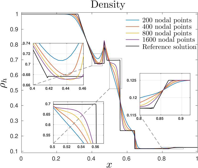
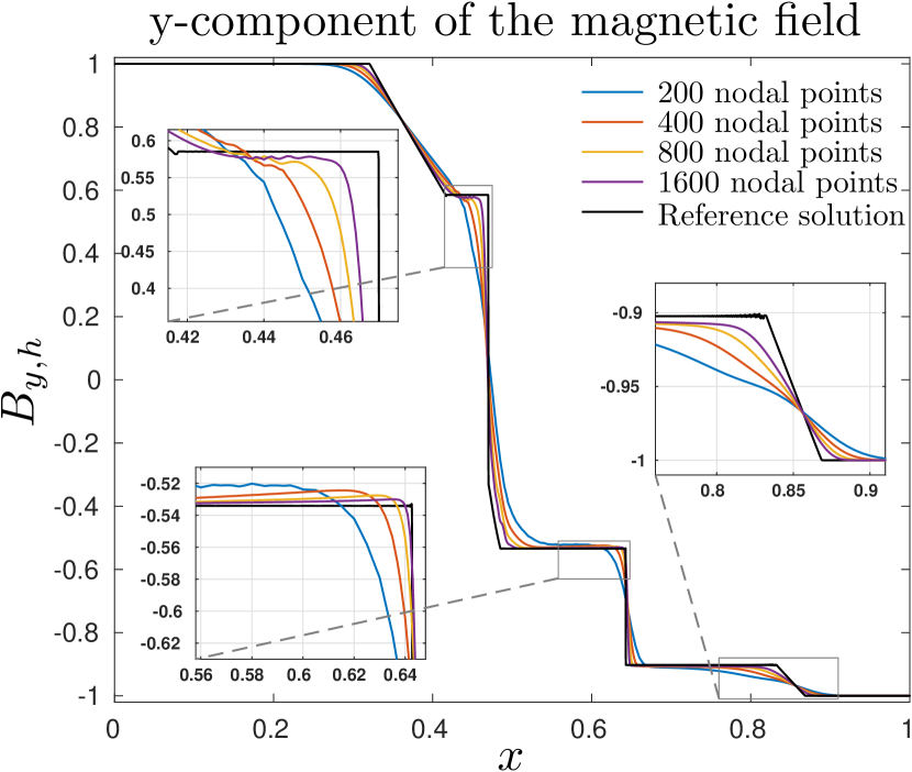
Figure 1: Density solution $\rho_{h}$ and the y-component of the magnetic field $\bm{\mathcal{B}}_{y,h}$ solution to the Brio-Wu problem using first-order viscosity. Note that even though the magnetic field has no viscous stabilization, the solution shows no significant unphysical oscillation.

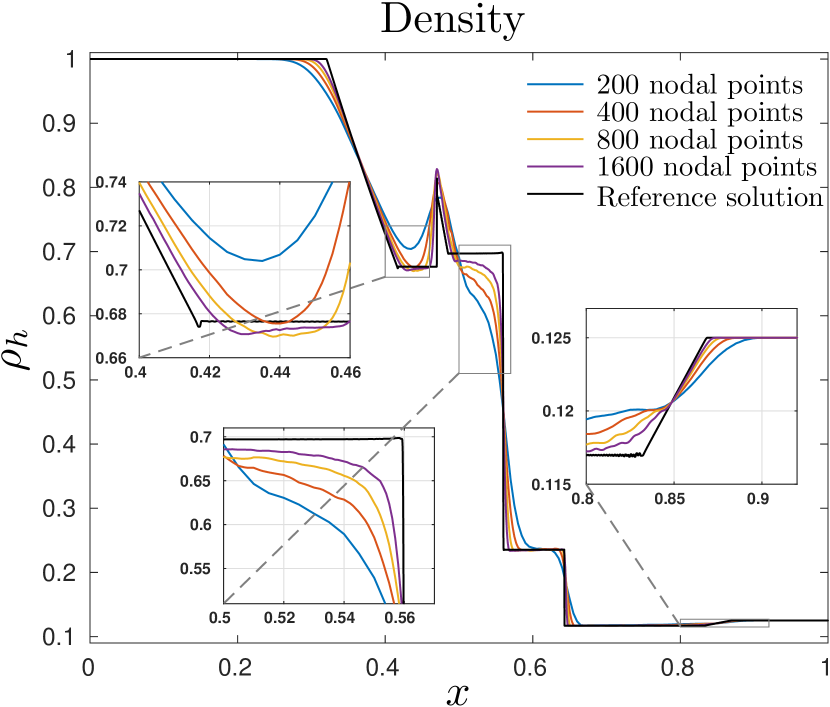
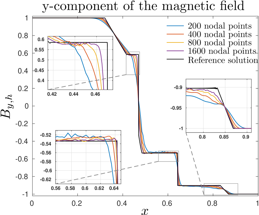
Figure 2: Density solution $\rho_{h}$ and the y-component of the magnetic field $\bm{\mathcal{B}}_{y,h}$ solution to the Brio-Wu problem using high-order entropy viscosity method. Just like any other second-order (or higher) accuracy scheme, some oscillations are to be expected. However, the natural expectation is that unphysical oscillations do not persist further refinement.

Table 4: Convergence rates of the density solution of the Brio-Wu problem using high-order entropy viscosity method

#nodes	L1	Rate	L2	Rate
100	3.11E-02	–	5.36E-02	–
200	1.89E-02	0.73	3.91E-02	0.46
400	1.17E-02	0.69	2.95E-02	0.41
800	7.17E-03	0.71	2.19E-02	0.43
1600	4.43E-03	0.69	1.62E-02	0.44

4.3 MHD Blast problem [3]

The domain is a square $[-0.5,0.5]\times[-0.5,0.5]$. Periodic boundary conditions are imposed in both $x-$ and $y-$ directions. The solution is initialized with an ambient fluid,

$$[\rho,\bm{v},p,\bm{\mathcal{B}}]^{\top}=\big{[}1,0,0,0.1,\tfrac{100}{\sqrt{4\pi}},0\big{]}^{\top}.$$

In the circle centered at the origin with radius $R=0.1$, the pressure is initialized at $p=1000$. The 10 000 times pressure difference creates a strong blast effect that is difficult for the numerical methods to capture. That is because the pressure can easily become negative due to approximation errors. The adiabatic gas constant is $\gamma=1.4$. The solution at $T=0.01$ is plotted in Figure 3. The obtained solutions agree well with the existing references, e.g., [3, 40, 41]. Detailed structures of the solution are visible, and no oscillatory behaviors are observed.

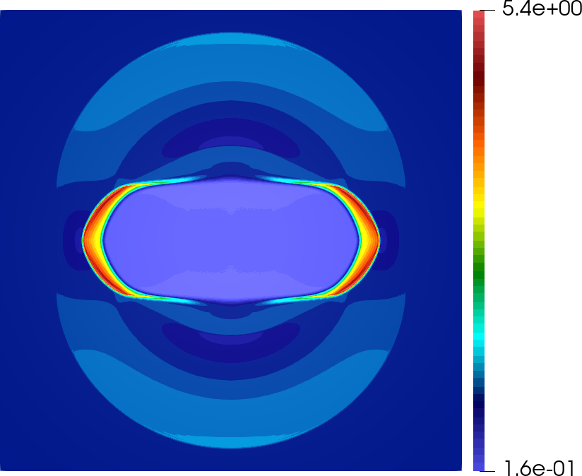
(a) Density $\rho_{h}$

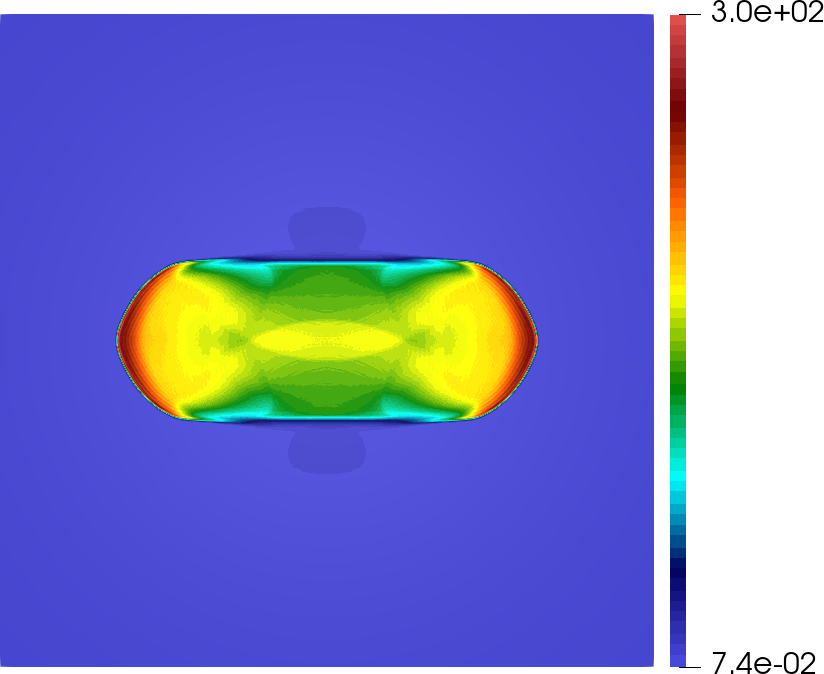
(b) Hydrodynamic pressure $p_{h}$

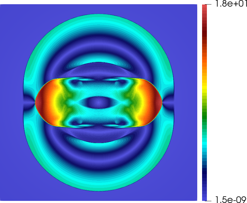
(c) Velocity magnitude $|\bm{v}_{h}|$

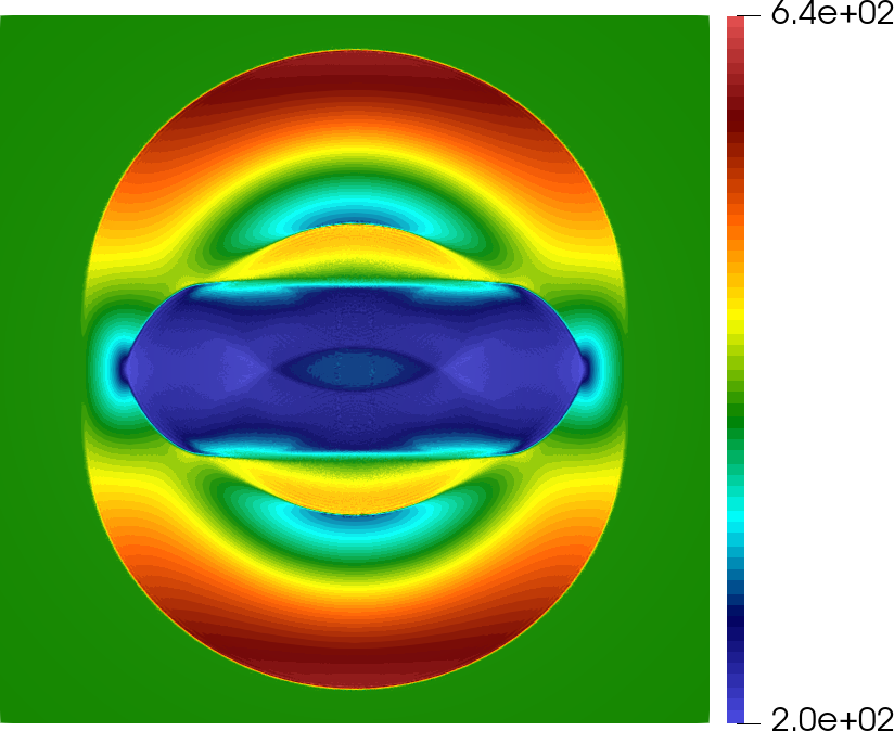
(d) Magnetic pressure $\bm{\mathcal{B}}_{h}^{2}/2$

Figure 3: Solution to Blast problem at time $t=0.01$ using 290147 nodal points

4.4 Astrophysical jet [40]

The last benchmark is proposed by [40]. The domain is $[-0.5,0.5]\times[0,1.5]$. The initial ambient fluid is given by

$$[\rho,\bm{v},p,\bm{\mathcal{B}}]^{\top}=[0.1\gamma,0,0,1.0,0,B_{a}]^{\top}.$$

A Mach 800 inflow is set on the inlet boundary $\bm{x}\in(-0.05,0,05)\times\{0\}$:

$$[\rho,\bm{v}]=[\gamma,0,800]^{\top}.$$

The adiabatic gas constant $\gamma=1.4$. The solution is simulated on half the domain and reflecting boundary condition is imposed on the line $x=0$. The Euler counterpart of this Mach 800 jet is already a very difficult test of positivity preservation of numerical schemes. Fortunately, we have a good Euler solver which can overcome this difficulty. Since the magnetic component is not present in the mechanical pressure, positivity of pressure in the split form is not interfered by how the magnetic field is. We observe that our method performs very well regardless of how extreme the magnetic field is. The solution is shown in Figure 4 when setting $B_{a}=\sqrt{200}$ and 5 when setting $B_{a}=\sqrt{20000}$. In Figure 4(b), we notice that the magnetic pressure is sharp but less smooth in some regions. This can be due to the fact that the magnetic field is not regularized. Since we did not implement out flow boundary conditions, the domain is extended to the directions of the bow shocks. The extended domain parts are cut out from the final plots.

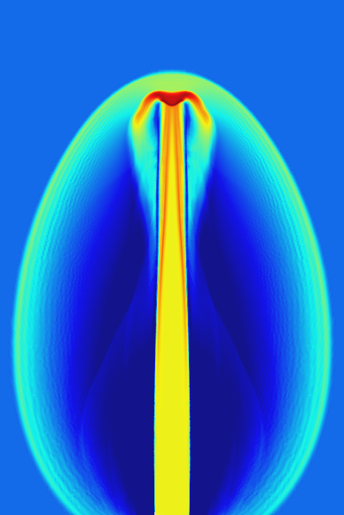
(a) Density logarithm $\log_{10}(\rho_{h})$

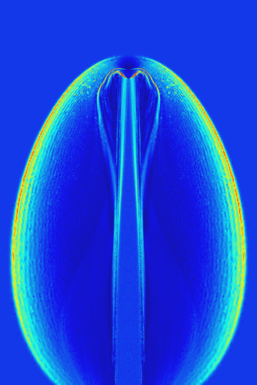
(b) Magnetic pressure $\bm{\mathcal{B}}_{h}^{2}/2$

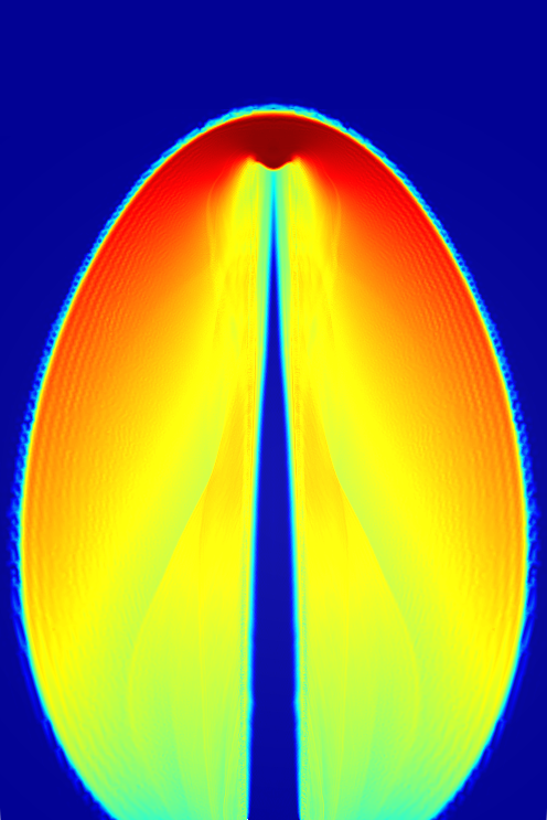
(c) Pressure logarithm $\log_{10}(p_{h})$

Figure 4: Solution to the astrophysical jet problem at time $t=0.002$, $B_{a}=\sqrt{200}$ using 136173 nodal points

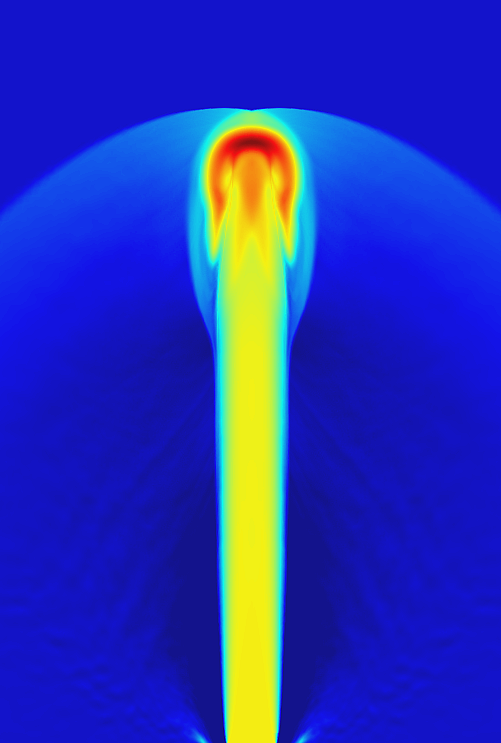
(a) Density logarithm $\log_{10}(\rho_{h})$

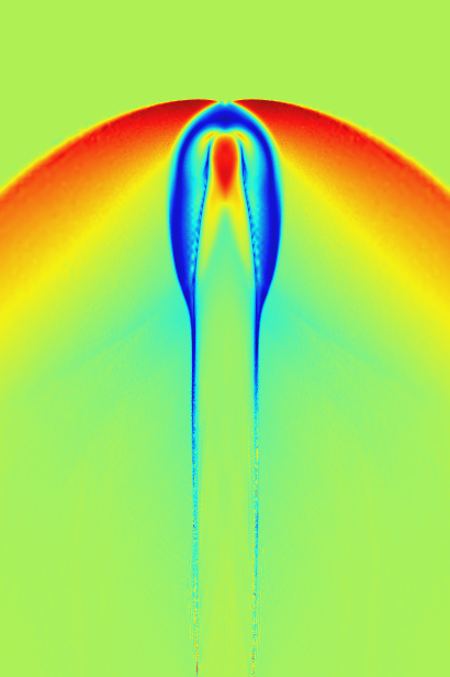
(b) Magnetic pressure $\bm{\mathcal{B}}_{h}^{2}/2$

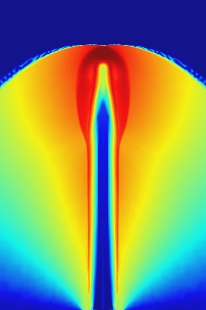
(c) Pressure logarithm $\log_{10}(p_{h})$

Figure 5: Solution to the astrophysical jet problem at time $t=0.002$, $B_{a}=\sqrt{20000}$ using 136173 nodal points

Remark 4.1 (Solver performance: Why is the scheme competitive?).

Implicit-time integration requires the execution of Newton iterations, with each iteration involving the inversion a Jacobian. In addition, the inverse of the Jacobian is applied using a Krylov method, with each iteration involving two matrix-vector products. The fundamental question of whether implicit time-integration is competitive (or not) boils down to having a low count of (linear and nonlinear) iterations. For the method advanced in this paper we have rather exceptional linear and nonlinear solver performance. For starters, the nonlinear system (44) is solved with at most 4 Newton iterations: we hardcoded the logic to stop the whole computation if more than 4 iterations are needed. This is in big part because we are using the solution from the previous time-step as an initial guess. On the other hand, even though the method does not have to respect the CFL of the MHD system, and magnetosonic waves can be ignored, we still have to respect the CFL of Euler system. Therefore the time-step sizes are still moderate and the resulting Jacobian is just a perturbation of the mass matrix. This means that an inexpensive Krylov method, such as BiCGStab without any form of preconditioning, can be used in practice. Usually less than a dozen matrix-vector product are used in order to apply the inverse of the Jacobian. We believe that the scheme is quite competitive and the incorporation of matrix-free linear algebra for system (44) would make the current implementation suitable to execute three-dimensional computations.

Appendix A Hyperbolic solver used in this paper

This section provides a brief outline of the numerical methods used to solve Euler’s system for all the computational experiments advanced in Section 4. The Euler’s system solver presented in this section fills in the role of euler_system_update invoked in Algorithm 3, which is supposed to comply with the properties described in Section 3.2. This section does not introduce any novel concept, idea, or numerical scheme, and it is only provided for the sake of completeness. The main ideas advanced in this section were originally developed in the sequence of papers [17, 16, 14] and references therein.

A.1 Low-order scheme

Low-order scheme is obtained using first-order Graph Viscosity method suggested first in [17]. Let $t_{n}$ be the current time, $\tau_{n}$ is the current time-step and we advance in time by setting $t_{n+1}=t_{n}+\tau_{n}$. Let $\bm{u}_{h}^{n}=\sum_{i\in\mathcal{V}_{\mathbb{V}}}\bm{u}_{i}^{n}\phi_{i}(\bm{x})$ be the finite element approximation at time $t_{n}$. The first order approximation at time $t_{n+1}$ is computed as

$$m_{i}\frac{\bm{u}_{i}^{\text{L},n+1}-\bm{u}_{i}^{n}}{\tau_{n}}+\sum_{j\in\mathcal{I}(i)}\bm{\mathbb{f}}(\bm{u}_{j}^{n})\mathbf{c}_{ij}-d_{ij}^{\text{L}}(\bm{u}_{j}^{n}-\bm{u}_{i}^{n})=\bm{0},$$ (52)

where $m_{i}$ and $\mathbf{c}_{ij}$ were defined in (32), while the set $\mathcal{I}(i)$ is the so-called stencil, which is defined as $\mathcal{I}(i)=\big{\{}j\in\mathcal{V}_{\mathbb{V}}\,|\,\mathbf{c}_{ij}\not=\bm{0}\big{\}}$, while the low-order graph-viscosity $d_{ij}^{\text{L}}$ is computed as

$$d_{ij}^{\text{L}} :=\max(\lambda_{\max}(\bm{u}_{i}^{n},\bm{u}_{j}^{n},\bm{n}_{ij})\,|\mathbf{c}_{ij}|_{\ell_{2}},\ \lambda_{\max}(\bm{u}_{j}^{n},\bm{u}_{i}^{n},\bm{n}_{ji})\,|\mathbf{c}_{ji}|_{\ell_{2}}),\quad\forall i\not=j,$$ (53)

$$d_{ii}^{\text{L}} :=-\sum_{i\not=j\in\mathcal{V}_{\mathbb{V}}}d_{ji}^{\text{L}}\ \ \text{and}\ \ \bm{n}_{ij}=\frac{\mathbf{c}_{ij}}{|\mathbf{c}_{ij}|_{\ell_{2}}}.$$

Here $\lambda_{\max}(\bm{u}_{L},\bm{u}_{R},\bm{n})$ is the maximum wave speed of the one dimensional Riemann problem: $\partial_{t}\bm{u}+\partial_{x}(\mathbf{f}(\bm{u})\bm{n})=0$, where $x=\bm{x}\cdot\bm{n}$, with initial condition: $\bm{u}(x,0)=\bm{u}_{L}=[\rho_{L},\bm{m}_{L},E_{L}]^{\top}$ if $x<0$, and $\bm{u}(x,0)=\bm{u}_{R}=[\rho_{R},\bm{m}_{R},E_{R}]^{\top}$ if $x\geq 0$. The maximum wavespeed of this Riemann problem can be computed exactly [38, Chap. 4], however this comes at the expense of solving a nonlinear problem. In theory and practice, any upper bound of the maximum wavespeed of the Riemann problem could be used in formula (53) while still preserving rigorous mathematical properties of the scheme [17, 18]. For the specific case of the covolume equation of state; $p(1-b\rho)=(\gamma-1)e\rho$ with $b\geq 0$; we can use $\lambda^{\#}(\bm{u}_{L},\bm{u}_{R},\mathbf{n})$ which is defined by

$$\lambda^{\#}(\bm{u}_{L},\bm{u}_{R},\mathbf{n})=\max((\lambda_{1}^{-}(p^{\#}))_{-},\ (\lambda_{3}^{+}(p^{\#}))_{+}),$$

$$\lambda_{1}^{-}(p^{\#})=v_{L}-c_{L}\left(1+\frac{\gamma+1}{2\gamma}\left(\frac{p^{\#}-p_{L}}{p_{L}}\right)_{+}\right)^{\frac{1}{2}},$$

$$\lambda_{3}^{+}(p^{\#})=v_{R}+c_{R}\left(1+\frac{\gamma+1}{2\gamma}\left(\frac{p^{\#}-p_{R}}{p_{R}}\right)_{+}\right)^{\frac{1}{2}},$$

$$p^{\#}:=\left(\frac{c_{L}(1-b\rho_{L})+c_{R}(1-b\rho_{R})-\frac{\gamma-1}{2}(v_{R}-v_{L})}{c_{L}(1-b\rho_{L})\ p_{L}^{-\frac{\gamma-1}{2\gamma}}+c_{R}(1-b\rho_{R})\ p_{R}^{-\frac{\gamma-1}{2\gamma}}}\right)^{\frac{2\gamma}{\gamma-1}},$$ (54)

where $z_{-}:=\max(0,-z)$, $z_{+}:=\max(0,z)$, $v_{L}=\bm{v}_{L}\cdot\bm{n}$, $v_{R}=\bm{v}_{R}\cdot\bm{n}$, $p_{L}$ and $p_{R}$ are the left and right pressures, and $c_{L}$ and $c_{R}$ are left and right sound speeds. Here the formula (54) is often referred to as the two-rarefaction estimate [38]. It is possible to show that $\lambda_{\max}(\bm{u}_{L},\bm{u}_{R},\mathbf{n})\leq\lambda^{\#}(\bm{u}_{L},\bm{u}_{R},\mathbf{n})$ [16] for $1<\gamma\leq\frac{5}{3}$. For all computations presented in this paper, $\lambda^{\#}(\bm{u}_{L},\bm{u}_{R},\mathbf{n})$ is used instead of $\lambda_{\max}(\bm{u}_{L},\bm{u}_{R},\bm{n})$ in order to compute the algebraic viscosities described in (53). We finally mention that scheme (52) equipped with the viscosity (53), is compatible with the assumption (41).

Remark A.1 (Convex reformulation and CFL condition).

The scheme (52) can be rewritten as

$$\bm{u}_{i}^{n+1}=\Big{(}1-\sum_{j\in\mathcal{I}(i)\backslash\{i\}}\tfrac{2\tau_{n}d_{ij}^{\textrm{L},n}}{m_{i}}\Big{)}\,\bm{u}_{i}^{n}+\sum_{j\in\mathcal{I}(i)\backslash\{i\}}\Big{(}\tfrac{2\tau_{n}d_{ij}^{\textrm{L},n}}{m_{i}}\Big{)}\,\overline{\bm{u}}_{ij}^{n},$$ (55)

where

$$\overline{\bm{u}}_{ij}^{n}=\tfrac{1}{2}(\bm{u}_{j}^{n}+\bm{u}_{i}^{n})-\tfrac{|\mathbf{c}_{ij}|}{2d_{ij}^{\textrm{L}}}(\bm{\mathbb{f}}(\bm{u}_{j}^{n})-\bm{\mathbb{f}}(\bm{u}_{i}^{n}))\bm{n}_{ij}$$ (56)

are the so-called bar-states. We note that the states $\{\overline{\bm{u}}_{ij}^{n}\}_{j\in\mathcal{I}(i)}$ are admissible provided that $\bm{u}_{i}^{n}$ and $\bm{u}_{j}^{n}$ are admissible and that $d_{ij}^{\textrm{L}}\geq\max(\lambda_{\max}(\bm{u}_{i}^{n},\bm{u}_{j}^{n},\bm{n}_{ij})\,\|\mathbf{c}_{ij}\|_{\ell_{2}},\ \lambda_{\max}(\bm{u}_{j}^{n},\bm{u}_{i}^{n},\bm{n}_{ji})\,\|\mathbf{c}_{ji}\|_{\ell_{2}})$, see [17, 18]. We note that $\bm{u}_{i}^{n+1}$ is a convex combination of the bar-states $\{\overline{\bm{u}}_{ij}^{n}\}_{j\in\mathcal{I}(i)}$ provided the condition $\Big{(}1-\sum_{j\in\mathcal{I}(i)\backslash\{i\}}\tfrac{2\tau_{n}d_{ii}^{\textrm{L},n}}{m_{i}}\Big{)}\geq 0$ holds. Therefore, we define the largest admissible time-step size as

$$\tau_{n}=\text{CFL}\cdot\min_{i\in\mathcal{V}_{\mathbb{V}}}\big{(}-\tfrac{m_{i}}{2d_{ii}^{\textrm{L},n}}\big{)}$$

where $\text{CFL}\in(0,1)$ is a user defined parameter.

A.2 High-order scheme

We note that the scheme (52) can only be first-order accurate. Therefore we consider the high-order scheme:

$$\sum_{j\in\mathcal{I}(i)}m_{ij}\frac{\bm{u}_{j}^{\text{{H}},n+1}-\bm{u}_{j}^{n}}{\tau_{n}}+\sum_{j\in\mathcal{I}(i)}\bm{\mathbb{f}}(\bm{u}_{j}^{n})\mathbf{c}_{ij}-d_{ij}^{\textrm{H}}(\bm{u}_{j}^{n}-\bm{u}_{i}^{n})=\bm{0},$$ (57)

Here $\{d_{ij}^{\textrm{H}}\}_{j\in\mathcal{I}(i)}$ are the high-order viscosities which are meant to be such that $d_{ij}^{\textrm{H}}\approx 0$ in smooth regions of the domain, while $d_{ij}^{\textrm{H}}\approx d_{ij}^{\textrm{L}}$ near shocks and discontinuities. In addition, $d_{ij}^{\textrm{H}}$ must be symmetric and conservative, i.e., $d_{ij}^{\textrm{H}}=d_{ji}^{\textrm{H}}$ and $d_{ii}^{\textrm{H}}:=-\sum_{i\not=j\in\mathcal{V}_{\mathbb{V}}}d_{ji}^{\textrm{H}}$.

In this paper, we use a high-order viscosity that is proportional to the entropy residual (i.e. entropy-production) of the unstabilized scheme. Let us start by considering the Galerkin solution $\bm{u}_{h}^{\text{G}}$ defined as

$$m_{i}\frac{\bm{u}_{i}^{\text{G}}-\bm{u}_{i}^{n}}{\tau_{n}}+\sum_{j\in\mathcal{I}(i)}\bm{\mathbb{f}}(\bm{u}_{j}^{n})\mathbf{c}_{ij}=\bm{0}\ \text{ for all }i\in\mathcal{V}_{\mathbb{V}}.$$ (58)

Let $\{\eta(\bm{u}),\bm{\mathbb{q}}(\bm{u})\}$ be an entropy pair of the Euler system. We define the entropy residual function $R^{n}_{h}(\bm{u}_{h})=\sum_{i\in\mathcal{V}_{\mathbb{V}}}R_{i}^{n}\phi_{i}\in\mathbb{V}_{h}$ with nodal values $R_{i}^{n}$ defined by

$$R_{i}^{n}:=m_{i}\frac{\bm{u}_{i}^{\text{G}}-\bm{u}_{i}^{n}}{\tau_{n}}\cdot\nabla_{\bm{u}}\eta(\bm{u}_{i}^{n})+\sum_{j\in\mathcal{I}(i)}\bm{\mathbb{q}}(\bm{u}_{j}^{n})\mathbf{c}_{ij}\ \text{ for all }i\in\mathcal{V}_{\mathbb{V}}.$$ (59)

Here $R_{i}^{n}$ is proportional to the entropy production of the unstabilized scheme (58). However, formula (59) is not practical, since it requires computing $\bm{u}_{i}^{\text{G}}$. We derive a formula for $R_{i}^{n}$ that does not invoke $\bm{u}_{i}^{\text{G}}$: multiplying (58) by $\nabla_{\bm{u}}\eta(\bm{u}_{i}^{n})$ we get that

$$m_{i}\frac{\bm{u}_{i}^{\text{G}}-\bm{u}_{i}^{n}}{\tau_{n}}\cdot\nabla_{\bm{u}}\eta(\bm{u}_{i}^{n})=-\sum_{j\in\mathcal{I}(i)}(\bm{\mathbb{f}}(\bm{u}_{j}^{n})\mathbf{c}_{ij})\cdot\nabla_{\bm{u}}\eta(\bm{u}_{i}^{n})$$

which we use to replace the first term in (59):

$$R_{i}^{n}=\sum_{j\in\mathcal{I}(i)}-(\bm{\mathbb{f}}(\bm{u}_{j}^{n})\mathbf{c}_{ij})\cdot\nabla_{\bm{u}}\eta(\bm{u}_{i}^{n})+\bm{\mathbb{q}}(\bm{u}_{j}^{n})\mathbf{c}_{ij}\text{ for all }i\in\mathcal{V}_{\mathbb{V}}.$$ (60)

In practice, we use (60) in order to compute the entropy-viscosity indicators. We are now ready to define the high-order nonlinear viscosity as

$$d_{ij}^{\textrm{H}}:=\min\Big{(}d_{ij}^{\textrm{L}},c_{\text{EV}}\max(\widetilde{R}^{n}_{i},\widetilde{R}^{n}_{j})\Big{)},$$

where $c_{\text{EV}}$ is a tunable constant, which is taken to be equal to 1 in numerical examples in this manuscript, and $\widetilde{R}^{n}_{i}$ is the normalized entropy residual:

$$\widetilde{R}^{n}_{i}:=\frac{R^{n}_{i}}{\max\Big{(}\rho^{\max,\,n}_{i}s^{\max,\,n}_{i}-\rho^{\min,\,n}_{i}s^{\min,\,n}_{i},\epsilon\|\eta^{n}_{h}\|_{L^{\infty}(\Omega)}\Big{)}},$$

where $w^{\max,\,n}_{i}:=\max_{j\in\mathcal{I}(i)}w^{n}_{j}$, and $w^{\min,\,n}_{i}:=\min_{j\in\mathcal{I}(i)}w^{n}_{j},$ for $w$ being $\rho$ or $s$. Recall that the mathematical entropy is computed as $\eta(\bm{u})=-\rho s(\bm{u})$, where $s(\bm{u})=\frac{1}{\gamma-1}\log(e)-\log(\rho)$ is the specific entropy. A small safety factor $\epsilon=10^{-8}$ is used to avoid division by zero.

A.3 Convex limiting

The low-order and high-order methods can be convenient rewritten as

$$m_{i}\big{(}\bm{u}_{i}^{\textrm{L},n+1}-\bm{u}_{i}^{n}\big{)}+\sum_{j\in\mathcal{I}(i)}\mathbf{F}_{ij}^{\textrm{L}}=\bm{0}\ \ \ \text{and}\ \ \ m_{i}\big{(}\bm{u}_{i}^{\textrm{H},n+1}-\bm{u}_{i}^{n}\big{)}+\sum_{j\in\mathcal{I}(i)}\mathbf{F}_{ij}^{\textrm{H}}=\bm{0}$$

where the algebraic fluxes $\mathbf{F}_{ij}^{\textrm{L}}$ are defined as $\mathbf{F}_{ij}^{\textrm{H}}$

$$\mathbf{F}_{ij}^{\textrm{L}} =\tau_{n}\big{(}\bm{\mathbb{f}}(\bm{u}_{j}^{n})+\bm{\mathbb{f}}(\bm{u}_{i}^{n})\big{)}\mathbf{c}_{ij}-\tau_{n}d_{ij}^{\textrm{L},n}(\bm{u}_{j}^{n}-\bm{u}_{i}^{n}),$$

$$\mathbf{F}_{ij}^{\textrm{H}} =\tau_{n}\big{(}\bm{\mathbb{f}}(\bm{u}_{j}^{n})+\bm{\mathbb{f}}(\bm{u}_{i}^{n})\big{)}\mathbf{c}_{ij}-\tau_{n}d_{ij}^{\textrm{H}}(\bm{u}_{j}^{n}-\bm{u}_{i}^{n})$$

$$\qquad+(m_{ij}-\delta_{ij}m_{i})(\bm{u}_{j}^{\textrm{H},n+1}-\bm{u}_{j}^{n}-\bm{u}_{i}^{\textrm{H},n+1}+\bm{u}_{i}^{n}).$$

We define the algebraic flux-corrections $\mathbf{A}_{ij}=\mathbf{F}_{ij}^{\textrm{L}}-\mathbf{F}_{ij}^{\textrm{H}}$ and set the final flux-limited solution to be

$$\begin{split}m_{i}\bm{u}_{i}^{n+1}=m_{i}\bm{u}_{i}^{\textrm{L},n+1}+\sum_{j\in\mathcal{I}(i)}\ell_{ij}\mathbf{A}_{ij}\end{split}$$ (61)

where $\ell_{ij}\in[0,1]$ are the limiters. If $\ell_{ij}\equiv 0$ for all $i$ and $j$, then (61) recovers $\bm{u}_{i}^{n+1}=\bm{u}_{i}^{\textrm{L},n+1}$. Similarly, if $\ell_{ij}\equiv 1$ for all $i$ and $j$ then (61) leads to $\bm{u}_{i}^{n+1}=\bm{u}_{i}^{\textrm{H},n+1}$. The goal is to select limiters as large as it could be possible while also preserving important bounds.

We want to enforce local bounds on the density and local minimum principle of the specific entropy. However, logarithmic entropies, such as $s(\bm{u})=\ln\frac{p(\bm{u})}{\rho^{\gamma}}$, are not friendly in the context Newton-like line search iterative methods. Therefore, we use $\tilde{s}(\bm{u})=\rho^{-\gamma}\varepsilon(\bm{u})$ which leads to an entirely equivalent minimum principle since

$$s(\bm{u})\leq s(\bm{v})\ \Leftrightarrow\ \tilde{s}(\bm{u})\leq\tilde{s}(\bm{v})\ \text{for all}\ \bm{u},\bm{v}\in\mathcal{A}\,,$$

due to the monotonicity of $\ln x$. Therefore, at each node $i\in\mathcal{V}_{\mathbb{V}}$ we compute the bounds:

$$\rho_{i}^{\text{min}} :=\mathbb{1}_{h}^{-}\min_{j\in\mathcal{I}(i)}\min\{\rho_{j}^{n},\overline{\rho}_{ij}^{n}\}$$

$$\rho_{i}^{\text{max}} :=\mathbb{1}_{h}^{+}\max_{j\in\mathcal{I}(i)}\max\{\rho_{j}^{n},\overline{\rho}_{ij}^{n}\}$$

$$\tilde{s}_{i}^{\text{min}} :=\mathbb{1}_{h}^{-}\min_{j\in\mathcal{I}(i)}\min\{\tilde{s}_{j}^{n},\overline{\tilde{s}}_{ij}^{n}\}$$

where $\overline{\rho}_{ij}^{n}$ denotes the density of the bar-state $\overline{\bm{u}}_{ij}^{n}$ (see expression (56)), while $\overline{\tilde{s}}_{ij}^{n}:=\tilde{s}(\overline{\bm{u}}_{ij}^{n})$. Here $\mathbb{1}_{h}^{-}$ and $\mathbb{1}_{h}^{+}$ are just ad-hoc relaxations of the unity with a prescribed decay rate with respect to the local meshsize $h$. More precisely we consider

$$\mathbb{1}_{h}^{-}=1-\kappa(\tfrac{m_{i}}{|\Omega|})^{\frac{p}{d}}\ \ \text{and}\ \ \mathbb{1}_{h}^{+}=1+\kappa(\tfrac{m_{i}}{|\Omega|})^{\frac{p}{d}}\ \ \text{with}\ p=1.50,\ d=2.0,\ \text{and}\ \kappa=4.0\,.$$

We mention in passing that, asymptotically for $h\rightarrow 0$, the value of $\kappa$ is has no importance and we may use any other $\kappa=\mathcal{O}(1)$. At each node $i\in\mathcal{V}_{\mathbb{V}}$ we define the set

$$\mathcal{B}_{i}=\big{\{}\bm{u}=[\rho,\bm{m},E]^{\top}\in\mathbb{R}^{d+2}\,\big{|}\,\rho_{i}^{\text{min}}\leq\rho\leq\rho_{i}^{\text{max}},\tilde{s}(\bm{u})\geq\tilde{s}_{i}^{\text{min}}\big{\}}$$

We note that (61) can be conveniently rewritten as

$$\begin{split}\bm{u}_{i}^{\textrm{H},n+1}=\sum_{j\in\mathcal{I}(i)}\lambda_{i}(\bm{u}_{i}^{\textrm{L},n+1}+\ell_{ij}\mathbf{P}_{ij})\ \ \text{where}\ \ \lambda_{i}=\tfrac{1}{\text{card}\mathcal{I}(i)-1}\ \ \text{and}\ \ \mathbf{P}_{ij}=\tfrac{1}{\lambda_{i}m_{i}}\mathbf{A}_{ij}\end{split}$$ (62)

Convex-limiting is built on the observation that condition $\bm{u}_{i}^{\textrm{H},n+1}\in\mathcal{B}_{i}$ will hold if $\bm{u}_{i}^{\textrm{L},n+1}+\ell_{ij}\mathbf{P}_{ij}\in\mathcal{B}_{i}$ for all $j\in\mathcal{I}(i)$. Therefore, at each node $i$ we compute the preliminary limiters $l_{ij}$ as

$$l_{ij}:=\texttt{compute\_line\_search}(\bm{u}_{i}^{\textrm{L},n+1},\mathbf{P}_{ij},\rho_{i}^{\text{min}},\rho_{i}^{\text{max}},\tilde{s}_{i}^{\text{min}})$$

with compute_line_search as defined in Algorithm 4, while the final limiters are computed as $\ell_{ij}=\min\{l_{ij},l_{ji}\}$ in order to guarantee conservation properties of the scheme, see [14, 13, 25] for both theory and implementation detail.

Algorithm 4 compute_line_search($\bm{u},\mathbf{P},\varrho^{\textit{min}},\varrho^{\textit{max}},\tilde{s}^{\textit{min}}$)

$$\ell^{\rho,\textit{min}}:=\max\{\ell\in[0,1]\,|\,\rho(\bm{u}+\ell\mathbf{P})\geq\varrho^{\textit{min}}\}$$

$$\ell^{\rho,\textit{max}}:=\max\{\ell\in[0,\ell^{\rho,\textit{min}}]\,|\,\rho(\bm{u}+\ell\mathbf{P})\leq\varrho^{\textit{max}}\}$$

$$\ell^{s}:=\max\{\ell\in[0,\ell^{\rho,\textit{max}}]\,|\,\tilde{s}(\bm{u}+\ell\mathbf{P})\geq\tilde{s}^{\textit{min}}\}$$

$$\texttt{Return:}\ell^{s}$$

Comments: input arguments are $\bm{u},\mathbf{P}\in\mathbb{R}^{m}$ and $\varrho^{\textit{min}},\varrho^{\textit{max}},\tilde{s}^{\textit{min}}\in\mathbb{R}^{+}$.

References

- [1] Douglas N Arnold and Anders Logg. Periodic table of the finite elements. Siam News, 47(9):212, 2014.
- [2] Franck Assous, Patrick Ciarlet, and Simon Labrunie. Mathematical foundations of computational electromagnetism, volume 198 of Applied Mathematical Sciences. Springer, Cham, 2018.
- [3] Dinshaw S. Balsara and Daniel S. Spicer. A staggered mesh algorithm using high order Godunov fluxes to ensure solenoidal magnetic fields in magnetohydrodynamic simulations. J. Comput. Phys., 149(2):270–292, 1999.
- [4] Melanie Basting and Dmitri Kuzmin. An FCT finite element scheme for ideal MHD equations in 1D and 2D. J. Comput. Phys., 338:585–605, 2017.
- [5] Nicolas Besse and Dietmar Kröner. Convergence of locally divergence-free discontinuous-Galerkin methods for the induction equations of the 2D-MHD system. M2AN Math. Model. Numer. Anal., 39(6):1177–1202, 2005.
- [6] Daniele Boffi, Franco Brezzi, and Michel Fortin. Mixed finite element methods and applications, volume 44 of Springer Series in Computational Mathematics. Springer, Heidelberg, 2013.
- [7] M. Brio and C. C. Wu. An upwind differencing scheme for the equations of ideal magnetohydrodynamics. J. Comput. Phys., 75(2):400–422, 1988.
- [8] Tuan Dao and Murtazo Nazarov. Monolithic parabolic regularization of the mhd equations and entropy principles. Comput. Methods Appl. Mech. Eng., 398:115269, 2022.
- [9] Tuan Anh Dao and Murtazo Nazarov. A high-order residual-based viscosity finite element method for the ideal MHD equations. J. Sci. Comput., 92(3):Paper No. 77, 24, 2022.
- [10] A. Dedner, F. Kemm, D. Kröner, C.-D. Munz, T. Schnitzer, and M. Wesenberg. Hyperbolic divergence cleaning for the MHD equations. J. Comput. Phys., 175(2):645–673, 2002.
- [11] Michael Fey and Manuel Torrilhon. A constrained transport upwind scheme for divergence-free advection. In Hyperbolic problems: theory, numerics, applications, pages 529–538. Springer, Berlin, 2003.
- [12] F. G. Fuchs, S. Mishra, and N. H. Risebro. Splitting based finite volume schemes for ideal MHD equations. J. Comput. Phys., 228(3):641–660, 2009.
- [13] Jean-Luc Guermond, Matthias Maier, Bojan Popov, and Ignacio Tomas. Second-order invariant domain preserving approximation of the compressible Navier-Stokes equations. Comput. Methods Appl. Mech. Engrg., 375:Paper No. 113608, 17, 2021.
- [14] Jean-Luc Guermond, Murtazo Nazarov, Bojan Popov, and Ignacio Tomas. Second-order invariant domain preserving approximation of the Euler equations using convex limiting. SIAM J. Sci. Comput., 40(5):A3211–A3239, 2018.
- [15] Jean-Luc Guermond and Bojan Popov. Viscous regularization of the Euler equations and entropy principles. SIAM J. Appl. Math., 74(2):284–305, 2014.
- [16] Jean-Luc Guermond and Bojan Popov. Fast estimation from above of the maximum wave speed in the Riemann problem for the Euler equations. J. Comput. Phys., 321:908–926, 2016.
- [17] Jean-Luc Guermond and Bojan Popov. Invariant domains and first-order continuous finite element approximation for hyperbolic systems. SIAM J. Numer. Anal., 54(4):2466–2489, 2016.
- [18] Jean-Luc Guermond, Bojan Popov, and Ignacio Tomas. Invariant domain preserving discretization-independent schemes and convex limiting for hyperbolic systems. Comput. Methods Appl. Mech. Engrg., 347:143–175, 2019.
- [19] Holger Heumann and Ralf Hiptmair. Stabilized Galerkin methods for magnetic advection. ESAIM Math. Model. Numer. Anal., 47(6):1713–1732, 2013.
- [20] Holger Heumann, Ralf Hiptmair, Kun Li, and Jinchao Xu. Fully discrete semi-Lagrangian methods for advection of differential forms. BIT, 52(4):981–1007, 2012.
- [21] Holger Heumann, Ralf Hiptmair, and Cecilia Pagliantini. Stabilized Galerkin for transient advection of differential forms. Discrete Contin. Dyn. Syst. Ser. S, 9(1):185–214, 2016.
- [22] Ralf Hiptmair and Cecilia Pagliantini. Splitting-based structure preserving discretizations for magnetohydrodynamics. SMAI J. Comput. Math., 4:225–257, 2018.
- [23] U. Koley, S. Mishra, N. H. Risebro, and M. Svärd. Higher-order finite difference schemes for the magnetic induction equations with resistivity. IMA J. Numer. Anal., 32(3):1173–1193, 2012.
- [24] Ujjwal Koley. Implicit finite difference scheme for the magnetic induction equation. In Hyperbolic problems—theory, numerics and applications. Volume 2, volume 18 of Ser. Contemp. Appl. Math. CAM, pages 478–485. World Sci. Publishing, Singapore, 2012.
- [25] Matthias Maier and Martin Kronbichler. Efficient parallel 3D computation of the compressible Euler equations with an invariant-domain preserving second-order finite-element scheme. ACM Trans. Parallel Comput., 8(3):Art. 16, 30, 2021.
- [26] Matthias Maier, John N. Shadid, and Ignacio Tomas. Structure-preserving finite-element schemes for the Euler-Poisson equations. Commun. Comput. Phys., 33(3):647–691, 2023.
- [27] Ralph Menikoff and Bradley J. Plohr. The riemann problem for fluid flow of real materials. Rev. Mod. Phys., 61:75–130, Jan 1989.
- [28] Siddhartha Mishra and Magnus Svärd. On stability of numerical schemes via frozen coefficients and the magnetic induction equations. BIT, 50(1):85–108, 2010.
- [29] Siddhartha Mishra and Eitan Tadmor. Constraint preserving schemes using potential-based fluxes. II. Genuinely multidimensional systems of conservation laws. SIAM J. Numer. Anal., 49(3):1023–1045, 2011.
- [30] Peter Monk. Finite element methods for Maxwell’s equations. Numerical Mathematics and Scientific Computation. Oxford University Press, New York, 2003.
- [31] Hans Christian Öttinger and Miroslav Grmela. Dynamics and thermodynamics of complex fluids. ii. illustrations of a general formalism. Physical Review E, 56(6):6633, 1997.
- [32] Benoit Perthame and Chi-Wang Shu. On positivity preserving finite volume schemes for Euler equations. Numer. Math., 73(1):119–130, 1996.
- [33] Tanmay Sarkar and Praveen Chandrashekar. Stabilized discontinuous Galerkin scheme for the magnetic induction equation. Appl. Numer. Math., 137:116–135, 2019.
- [34] Joel Smoller. Shock waves and reaction-diffusion equations, volume 258 of Grundlehren der mathematischen Wissenschaften [Fundamental Principles of Mathematical Sciences]. Springer-Verlag, New York, second edition, 1994.
- [35] James M Stone, Thomas A Gardiner, Peter Teuben, John F Hawley, and Jacob B Simon. Athena: a new code for astrophysical mhd. Astrophys. J., Suppl. Ser., 178(1):137, 2008.
- [36] Eitan Tadmor. A minimum entropy principle in the gas dynamics equations. Appl. Numer. Math., 2(3-5):211–219, 1986.
- [37] K. Takahashi and S. Yamada. Regular and non-regular solutions of the riemann problem in ideal magnetohydrodynamics. Journal of Plasma Physics, 79(3):335–356, 2013.
- [38] Eleuterio F. Toro. Riemann solvers and numerical methods for fluid dynamics. Springer-Verlag, Berlin, third edition, 2009. A practical introduction.
- [39] M. Torrilhon and M. Fey. Constraint-preserving upwind methods for multidimensional advection equations. SIAM J. Numer. Anal., 42(4):1694–1728, 2004.
- [40] Kailiang Wu and Chi-Wang Shu. A provably positive discontinuous Galerkin method for multidimensional ideal magnetohydrodynamics. SIAM J. Sci. Comput., 40(5):B1302–B1329, 2018.
- [41] Kailiang Wu and Chi-Wang Shu. Provably positive high-order schemes for ideal magnetohydrodynamics: analysis on general meshes. Numer. Math., 142(4):995–1047, 2019.
- [42] Xiangxiong Zhang and Chi-Wang Shu. On positivity-preserving high order discontinuous Galerkin schemes for compressible Euler equations on rectangular meshes. J. Comput. Phys., 229(23):8918–8934, 2010.