Do Not Harm Protected Groups in Debiasing Language Representation Models
Abstract
Language Representation Models (LRMs) trained with real-world data may capture and exacerbate undesired bias and cause unfair treatment of people in various demographic groups. Several techniques have been investigated for applying interventions to LRMs to remove bias in benchmark evaluations on, for example, word embeddings. However, the negative side effects of debiasing interventions are usually not revealed in the downstream tasks. We propose xGAP-Debias, a set of evaluations on assessing the fairness of debiasing. In this work, We examine four debiasing techniques on a real-world text classification task and show that reducing biasing is at the cost of degrading performance for all demographic groups, including those the debiasing techniques aim to protect. We advocate that a debiasing technique should have good downstream performance with the constraint of ensuring no harm to the protected group.
1 Introduction
Suppose a hiring hospital wants to offer targeted advertisements for an open surgeon position. The employer from the hospital mines the user’s bio on social media to predict whether an individual is a surgeon to determine whether to offer the relevant advertisement. To make the prediction, they use a pre-trained Language Representation Model to encode the text and then fine-tune a classification model on top of the representation. The employer decides to use a debiasing technique on the mined data to give equal opportunity to people with different attributes. However, the employer observes that female surgeons receive the advertisement at much lower rates than male surgeons. Even worse, the fraction of female surgeons seeing the advertisement went down after the debiasing intervention. In this work, we show that such scenarios are highly plausible with existing debiasing techniques.
Undesired bias or social stereotypes have been found in natural language representations [4], and systematic ways of debiasing have been widely discussed [11, 2, 15, 5]. Recent works focus on developing techniques to detect, evaluate and mitigate bias in LRMs and reduce harm to marginalized individuals and groups [29, 13, 20, 15, 5, 17, 14]. Some of those works measure bias comprising metrics [13, 7] and datasets [1, 6] to investigate biases within a specific natural language processing (NLP) task, such as text classification [26] or language generation [21]. Other works design debiasing techniques for the specific applications in patient notes [16], clinical record de-identification [24], or dissecting ML-guided health decisions [18].
Due to the variants in datasets and the application area, it is hard to evaluate the downstream performance of the debiasing techniques. Previous work has raised this concern [19] by utilizing Equality of Opportunity and evaluating the downstream model performance with debiasing across all groups in the dataset. We expand this consideration to examine how debiasing affects group-wise performance and the model performance with other well-known debiasing techniques.
In this work, we study the effectiveness of the language debiasing technique on the task where the protected attributes are given in the dataset (Figure 11). We propose xGAP-Debias, a framework with a combination of criteria for characterizing fairness in multiple senses: a group-wise utility or performance measure (x) and the corresponding difference of performance x between groups (known as GAP) of model performance on that evaluation metrics between protected attributes. We evaluate four widely-used debiasing techniques on a challenging language model multiclass classification task, where the input is embedded from brief natural language bios, and the target of the classification is the profession. We find that debiasing techniques are either ineffective in reducing the GAP, or are effective at the cost of reducing the model performance on protected attributes, including the group for which debiasing was intended to improve outcomes. In a context where the protected group subject prefers higher model performance, such an intervention achieves ‘fairness’ only through harm.
2 xGAP-Debias
There are many diverse downstream applications for natural language classifiers, and as such, limit to any specific metric will likely have limited utility in some cases. Our xGAP-Debias leaves the flexibility to use any desired evaluation metric to match the use case at hand. The x can, therefore, be any performance evaluation metric used at the class level in the downstream task.
xGAP-Debias Fairness Definition. We argue that a fair debiasing technique should guarantee that after debiasing:
-
1.
Metrics (x) of the protected group111In this study, we define the ‘protected group’ as the demographic group with a lower performance before applying debiasing techniques. with respect to the protected attributes should be no worse than before. This can be thought of as a “do no harm” criterion.
-
2.
The GAP of the metrics between protected attributes should decrease substantially. This can be thought of as an “improvement in equality criterion.”
If a debiasing intervention satisfies these two criteria, we consider this base satisfaction. For a multi-class classification problem, we can further break down this criteria satisfaction at the level of individual predictive classes for each demographic group.
We say an intervention satisfies advanced satisfaction if, in addition to base satisfaction, it does not result in a reduction of performance (measured by x) for the non-protected group(s).
3 Experiment
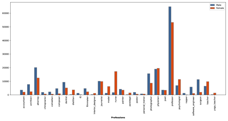
Data. In our study, we use Bias in Bios[1], which contains short online biographies (bios) written in English. Each bio is associated with one of 28 professions and one of two gender identities, where we consider the gender identity as ‘protected attributes’222We acknowledge that gender is more complex and non-binary. Following the data collection process in Bias in Bios, we used a binary division of gender while investigating the bias in the pre-trained language models and consider the gender group as the only group in all the experiments in this paper.. We want to predict a profession given the tokenized English bio. Details of the study population can be found in Figure 11.
Problem Statement. We want to evaluate the overall and group-wise prediction performance before and after applying each debiasing technique.
In both the overall and the group-wise evaluation, we consider the True Positive Rate (TPR) of the classification, broken down by gender, as the relevant utility measure x and calculate the difference of TPR between groups. Denote the set of all profession for each tokenized bio in the dataset . For the protected attribute in all attributes , in a given profession , we have binary gender attribute male () and female (). The GAP of TPR can be denoted as with a specific gender and profession prediction . For a given profession :
| (1) |
where , , and are predictions for the profession, gender, and ground-truth profession, respectively.
We use the GAP to measure the difference in model performance for the selected evaluation metric between the protected attributes, which quantifies the disparity in the model’s classification task performance prediction across different prediction classes and protected attributes.
In the overall performance evaluation, due to the data variance, we involve the idea of GAP Root Mean Square (GAPRMS) with TPR to combat the possible impact of data imbalance [20]. We denote the GAPRMS in this experiment as333For simplicity, in the rest of the paper, GAP refers to TPR GAP and GAPRMS refers to the TPR GAP with Root Mean Square.:
| (2) |
GAPRMS helps to evaluate both the model predictions and the variance with respect to different profession groups. Different from comparing the averaged group-wise TPR overall profession groups, GAPRMS will not be influenced by the imbalanced disparities in TPR in one attribute in one direction.
We use TPR and Accuracy in conjunction with the evaluation. Accuracy measures the proportion of correctly classified cases overall with the system, regardless of the specific classes the predicted label belongs to. Under extreme data imbalance cases, accuracy might not be an ideal pick of metrics for performance evaluation. Different from the group-wise population, the overall population of the protected attributes is close to each other and accuracy thus turns out to be a valuable metric x for the overall performance evaluation. Appendix D elaborates more on evaluation metrics and how they contribute to this experiment.
Experimental Setup. In this study, we evaluate the following four debiasing methods (Appendix A):
We use the Logistic Regression classifier with multi-group classification for prediction444For INLP, we tokenize the English bio with BERT [8]. To validate our results through statistical significance testing, we use the same set of hyperparameters on the classifier and repeat the experiment five times for each debiasing techniques. We report the mean performance across these runs and run a two-sample t-test to investigate if the difference between means is statistically significant.

Results. Table 1 presents the overall model performance before and after applying the four debiasing techniques. We observe that after debiasing, across all groups, the GAPRMS between the protected attributes decreases substantially. However, this comes at the expense of worsening the model prediction for both groups, including the protected group with worse-off performance before debiasing. The overall performance seems to satisfy the GAP criterion in xGAP-Debias while failing to achieve the first ‘do no harm’ criterion.
| Original | EO | Decoupled | CDA | INLP | |
|---|---|---|---|---|---|
| Accuracy | 79.89 | 72.81 7.08 | 79.87 0.02 | 79.79 0.10 | 78.14 1.75 |
| GAP | 15.65 | 11.98 3.67 | 15.61 0.04 | 14.15 1.50 | 12.11 3.54 |
| TPR | 80.58 | 73.35 7.23 | 80.57 0.01 | 80.56 0.02 | 78.90 1.68 |
| TPR | 78.70 | 71.41 7.29 | 78.67 0.03 | 78.51 0.19 | 76.77 1.93 |
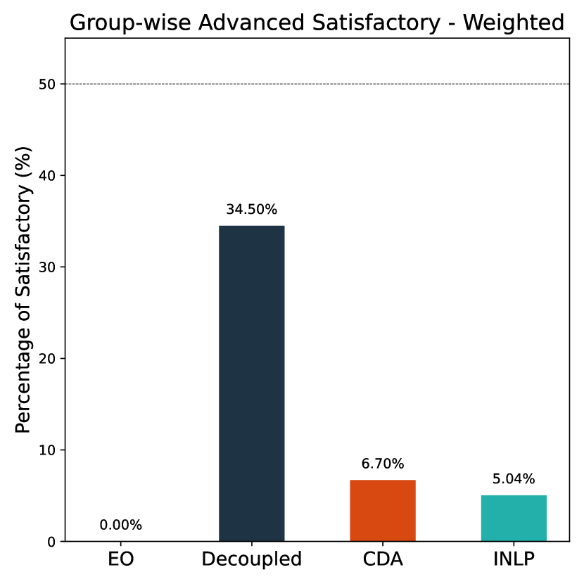
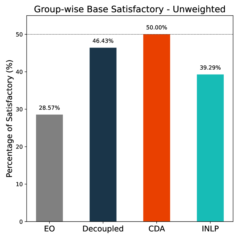
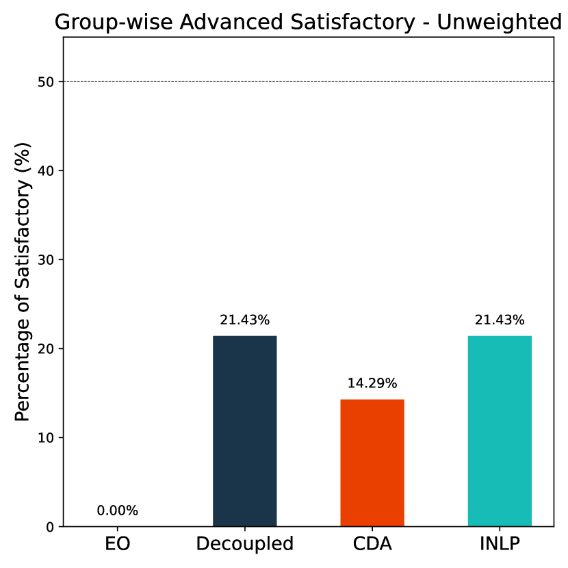
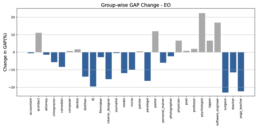
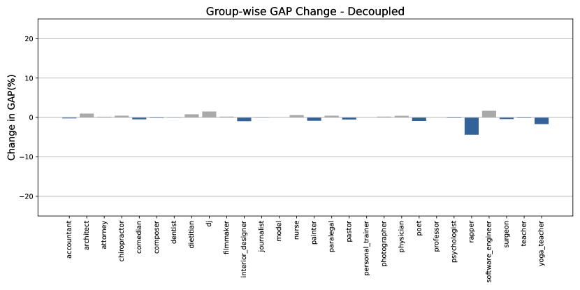
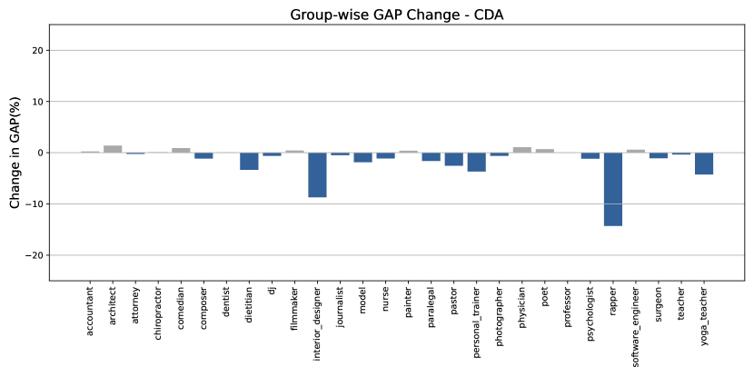
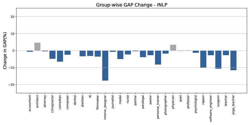
Appendix A details the performance after debiasing on each of the 28 professions for all four techniques. Among all the professions, INLP has more than 85% groups where the GAP decreases after debiasing (Table 6). Meanwhile, the change of GAP with INLP is also the best among all the debiasing techniques (Figure 10). We detail the change of TPR regarding the protected attributes in Appendix D. To address the impact of data imbalance, we consider both unweighted and weighted calculations with respect to the group population in evaluating the group-wise satisfaction rate among different professions (the prediction groups). Figure 2 shows base and advanced satisfaction with weighted and unweighted calculations. The weighted performance of the debiasing techniques is more distinctive than the unweighted. While the total number of satisfaction is similar, one technique might have the satisfaction on the profession with a large population. Decoupled Classifiers constantly outperform the other debiasing techniques, regardless of whether take total affected data points into consideration. Unfortunately, for all four debiasing techniques, none of them exceed 50% satisfaction rate under both base and advanced satisfaction criteria.
| Method | Worsened GAP |
|---|---|
| EO | 39% |
| Decoupled | 39% |
| CDA | 39% |
| INLP | 14% |
Figure 10 shows the changes in GAP broken down by profession. Note that while EO had the greatest improvement in GAP (Table 1), that performance increase is not equally spread across all professions. Likewise, Table 2 shows the percentage of professions that worsened in the GAP metric for each debiasing method. We observe that no method is able to achieve an overall reduction in GAP without increasing the GAP in a sizeable portion of the professions. In particular, EO, Decoupled, and CDA increase the GAP in more than a third of professions. This adds a new dimension of complexity to the analysis of reducing harm, which has not yet been explored.
4 Discussion
Our work introduces xGAP-Debias, a framework to evaluate the effectiveness and fairness of language debiasing models on specific downstream tasks. From the multiclass classification task, we investigate the fairness of debiasing models in different perspectives: we introduce base and advance xGAP-Debias rule of satisfaction, evaluate both overall and group-wise performance (Table 1, Appendix A), compare the weighted and unweighted satisfactions (Figure 2), and measured the proportion of groups that are harmed by increasing the overall performance (Table 2). From the result, we found that none of the debiasing models achieves over 50% xGAP-Debias satisfaction.
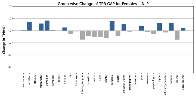
Among the four models, the Decoupled seems to have the best performance in satisfaction results. However, as we delve deep into the results of xGAP-Debias metrics, we found that in group-wise evaluation, the Decoupled does not have much improvements in reducing the GAP or increasing the TPR for the protected group (Figure 3, Figure 8). And INLP worsen about half of the professions in the TPR performance for the protected group (Figure 4). When examining the effects of these debiasing techniques, we see a further complexity not yet addressed in the literature. While all techniques cause a decrease in GAP metrics, this effect is not uniform across professions. As stated in [20], INLP is known for reducing GAP after debiasing. When we move one step deeper, from the overall performance to the group-wise performance, INLP hurts more than one-third of the groups to achieve a reduction of GAP in the report of overall performance (Table 2, Figure 10).
In the previous discussion, one might found that the model with high xGAP-Debias satisfaction is actually not doing the debiasing job well. One might question how xGAP-Debias assists in evaluating fair and effective language debiasing techniques. We advocate that xGAP-Debias should be considered as the first constraint in the debiasing evaluation. It means a debiasing model should guarantee to maintain a high satisfaction rate with xGAP-Debias before reaching the goal of improving the prediction performance. Therefore, a good debiasing technique should consider xGAP-Debias as to pass an ‘entry test’ to demonstrate the model robustness in fairness without harm to the protected group(s).

5 Conclusion and Future Work
In our study, we have highlighted difficulties with existing debiasing techniques when used as part of an intervention on a language classification task. Through xGAP-Debias, we highlight practical challenges that existing debiasing techniques face to remain ‘fair’ after debiasing in the downstream applications, such as a tradeoff in performance or imbalanced changes in performance across the target classes. There is a gap in the current state of the art for a principled debiasing technique that can guarantee higher satisfaction rates of both our ‘do no harm’ and ‘improvement of equality’ criteria. Our evaluation motivates the need for multiple assessments of fairness to ensure bias reduction without harm.
6 Social Impact Statement
The goal of debiasing is to intentionally tip the scale back in favor of those who face discrimination without inadvertently perpetuating harm or injustice. As pointed back to the hiring story, one may wish to debias the model toward the direction that the gap between men and women is reduced. However, the inadvertent effect might be that our model becomes an even poorer recruitment tool for finding surgeons, sacrificing the model performance for all protected attributes to have a closer prediction performance, even harming the very group we intended to increase equity. With the development of language technology, it is unavoidable to observe bias within the model. We are committed to advancing the research on reducing bias in language models, which requires more robust evaluations and frameworks for fairness.
References
- [1] Maria De-Arteaga, Alexey Romanov, Hanna Wallach, Jennifer Chayes, Christian Borgs, Alexandra Chouldechova, Sahin Geyik, Krishnaram Kenthapadi and Adam Tauman Kalai “Bias in bios: A case study of semantic representation bias in a high-stakes setting” In proceedings of the Conference on Fairness, Accountability, and Transparency, 2019, pp. 120–128
- [2] Emily M Bender, Timnit Gebru, Angelina McMillan-Major and Shmargaret Shmitchell “On the dangers of stochastic parrots: Can language models be too big? ” In Proceedings of the 2021 ACM conference on fairness, accountability, and transparency, 2021, pp. 610–623
- [3] Hugo Berg, Siobhan Hall, Yash Bhalgat, Hannah Kirk, Aleksandar Shtedritski and Max Bain “A Prompt Array Keeps the Bias Away: Debiasing Vision-Language Models with Adversarial Learning” In Proceedings of the 2nd Conference of the Asia-Pacific Chapter of the Association for Computational Linguistics and the 12th International Joint Conference on Natural Language Processing (Volume 1: Long Papers) Online only: Association for Computational Linguistics, 2022, pp. 806–822 URL: https://aclanthology.org/2022.aacl-main.61
- [4] Tolga Bolukbasi, Kai-Wei Chang, James Y Zou, Venkatesh Saligrama and Adam T Kalai “Man is to computer programmer as woman is to homemaker? debiasing word embeddings” In Advances in neural information processing systems 29, 2016
- [5] Aylin Caliskan, Joanna J Bryson and Arvind Narayanan “Semantics derived automatically from language corpora contain human-like biases” In Science 356.6334 American Association for the Advancement of Science, 2017, pp. 183–186
- [6] Ilias Chalkidis, Tommaso Pasini, Sheng Zhang, Letizia Tomada, Sebastian Schwemer and Anders Søgaard “FairLex: A Multilingual Benchmark for Evaluating Fairness in Legal Text Processing” In Proceedings of the 60th Annual Meeting of the Association for Computational Linguistics (Volume 1: Long Papers) Dublin, Ireland: Association for Computational Linguistics, 2022, pp. 4389–4406 DOI: 10.18653/v1/2022.acl-long.301
- [7] Paula Czarnowska, Yogarshi Vyas and Kashif Shah “Quantifying Social Biases in NLP: A Generalization and Empirical Comparison of Extrinsic Fairness Metrics” In Transactions of the Association for Computational Linguistics 9 Cambridge, MA: MIT Press, 2021, pp. 1249–1267 DOI: 10.1162/tacl˙a˙00425
- [8] Jacob Devlin, Ming-Wei Chang, Kenton Lee and Kristina Toutanova “BERT: Pre-training of Deep Bidirectional Transformers for Language Understanding” In Proceedings of the 2019 Conference of the North American Chapter of the Association for Computational Linguistics: Human Language Technologies, Volume 1 (Long and Short Papers) Minneapolis, Minnesota: Association for Computational Linguistics, 2019, pp. 4171–4186 DOI: 10.18653/v1/N19-1423
- [9] Yanai Elazar and Yoav Goldberg “Adversarial Removal of Demographic Attributes from Text Data” In Proceedings of the 2018 Conference on Empirical Methods in Natural Language Processing Brussels, Belgium: Association for Computational Linguistics, 2018, pp. 11–21 DOI: 10.18653/v1/D18-1002
- [10] Fuli Feng, Jizhi Zhang, Xiangnan He, Hanwang Zhang and Tat-Seng Chua “Empowering Language Understanding with Counterfactual Reasoning” In Findings of the Association for Computational Linguistics: ACL-IJCNLP 2021, 2021, pp. 2226–2236
- [11] Hila Gonen and Yoav Goldberg “Lipstick on a Pig: Debiasing Methods Cover up Systematic Gender Biases in Word Embeddings But do not Remove Them” In Proceedings of the 2019 Conference of the North American Chapter of the Association for Computational Linguistics: Human Language Technologies, Volume 1 (Long and Short Papers) Minneapolis, Minnesota: Association for Computational Linguistics, 2019, pp. 609–614 DOI: 10.18653/v1/N19-1061
- [12] Yue Guo, Yi Yang and Ahmed Abbasi “Auto-Debias: Debiasing Masked Language Models with Automated Biased Prompts” In Proceedings of the 60th Annual Meeting of the Association for Computational Linguistics (Volume 1: Long Papers) Dublin, Ireland: Association for Computational Linguistics, 2022, pp. 1012–1023 DOI: 10.18653/v1/2022.acl-long.72
- [13] Moritz Hardt, Eric Price and Nati Srebro “Equality of opportunity in supervised learning” In Advances in neural information processing systems 29, 2016
- [14] Tao Li, Daniel Khashabi, Tushar Khot, Ashish Sabharwal and Vivek Srikumar “UNQOVERing Stereotyping Biases via Underspecified Questions” In Findings of the Association for Computational Linguistics: EMNLP 2020 Online: Association for Computational Linguistics, 2020, pp. 3475–3489 DOI: 10.18653/v1/2020.findings-emnlp.311
- [15] Chandler May, Alex Wang, Shikha Bordia, Samuel R. Bowman and Rachel Rudinger “On Measuring Social Biases in Sentence Encoders” In Proceedings of the 2019 Conference of the North American Chapter of the Association for Computational Linguistics: Human Language Technologies, Volume 1 (Long and Short Papers) Minneapolis, Minnesota: Association for Computational Linguistics, 2019, pp. 622–628 DOI: 10.18653/v1/N19-1063
- [16] Joshua R Minot, Nicholas Cheney, Marc Maier, Danne C Elbers, Christopher M Danforth and Peter Sheridan Dodds “Interpretable bias mitigation for textual data: Reducing genderization in patient notes while maintaining classification performance” In ACM Transactions on Computing for Healthcare 3.4 ACM New York, NY, 2022, pp. 1–41
- [17] Nikita Nangia, Clara Vania, Rasika Bhalerao and Samuel R. Bowman “CrowS-Pairs: A Challenge Dataset for Measuring Social Biases in Masked Language Models” In Proceedings of the 2020 Conference on Empirical Methods in Natural Language Processing (EMNLP) Online: Association for Computational Linguistics, 2020, pp. 1953–1967 DOI: 10.18653/v1/2020.emnlp-main.154
- [18] Ziad Obermeyer, Brian Powers, Christine Vogeli and Sendhil Mullainathan “Dissecting racial bias in an algorithm used to manage the health of populations” In Science 366.6464 American Association for the Advancement of Science, 2019, pp. 447–453
- [19] Flavien Prost, Nithum Thain and Tolga Bolukbasi “Debiasing Embeddings for Reduced Gender Bias in Text Classification” In GeBNLP 2019 9573, 2019, pp. 69
- [20] Shauli Ravfogel, Yanai Elazar, Hila Gonen, Michael Twiton and Yoav Goldberg “Null It Out: Guarding Protected Attributes by Iterative Nullspace Projection” In Proceedings of the 58th Annual Meeting of the Association for Computational Linguistics Online: Association for Computational Linguistics, 2020, pp. 7237–7256 DOI: 10.18653/v1/2020.acl-main.647
- [21] Emily Sheng, Kai-Wei Chang, Premkumar Natarajan and Nanyun Peng “The Woman Worked as a Babysitter: On Biases in Language Generation” In Proceedings of the 2019 Conference on Empirical Methods in Natural Language Processing and the 9th International Joint Conference on Natural Language Processing (EMNLP-IJCNLP) Hong Kong, China: Association for Computational Linguistics, 2019, pp. 3407–3412 DOI: 10.18653/v1/D19-1339
- [22] Berk Ustun, Yang Liu and David Parkes “Fairness without harm: Decoupled classifiers with preference guarantees” In International Conference on Machine Learning, 2019, pp. 6373–6382 PMLR
- [23] Blake Woodworth, Suriya Gunasekar, Mesrob I Ohannessian and Nathan Srebro “Learning non-discriminatory predictors” In Conference on Learning Theory, 2017, pp. 1920–1953 PMLR
- [24] Yuxin Xiao, Shulammite Lim, Tom Joseph Pollard and Marzyeh Ghassemi “In the Name of Fairness: Assessing the Bias in Clinical Record De-identification” In Proceedings of the 2023 ACM Conference on Fairness, Accountability, and Transparency, 2023, pp. 123–137
- [25] Rich Zemel, Yu Wu, Kevin Swersky, Toni Pitassi and Cynthia Dwork “Learning fair representations” In International conference on machine learning, 2013, pp. 325–333 PMLR
- [26] Jieyu Zhao, Subhabrata Mukherjee, Saghar Hosseini, Kai-Wei Chang and Ahmed Hassan Awadallah “Gender Bias in Multilingual Embeddings and Cross-Lingual Transfer” In Proceedings of the 58th Annual Meeting of the Association for Computational Linguistics Online: Association for Computational Linguistics, 2020, pp. 2896–2907 DOI: 10.18653/v1/2020.acl-main.260
- [27] Jieyu Zhao, Tianlu Wang, Mark Yatskar, Vicente Ordonez and Kai-Wei Chang “Gender Bias in Coreference Resolution: Evaluation and Debiasing Methods” In Proceedings of the 2018 Conference of the North American Chapter of the Association for Computational Linguistics: Human Language Technologies, Volume 2 (Short Papers) New Orleans, Louisiana: Association for Computational Linguistics, 2018, pp. 15–20 DOI: 10.18653/v1/N18-2003
- [28] Kang Zhou, Yuepei Li and Qi Li “Distantly Supervised Named Entity Recognition via Confidence-Based Multi-Class Positive and Unlabeled Learning” In Proceedings of the 60th Annual Meeting of the Association for Computational Linguistics (Volume 1: Long Papers) Dublin, Ireland: Association for Computational Linguistics, 2022, pp. 7198–7211 DOI: 10.18653/v1/2022.acl-long.498
- [29] Ran Zmigrod, Sabrina J. Mielke, Hanna Wallach and Ryan Cotterell “Counterfactual Data Augmentation for Mitigating Gender Stereotypes in Languages with Rich Morphology” In Proceedings of the 57th Annual Meeting of the Association for Computational Linguistics Florence, Italy: Association for Computational Linguistics, 2019, pp. 1651–1661 DOI: 10.18653/v1/P19-1161
Appendix A Profession-Level Model Performance
We provide more details about group-wise model performance for each of the debiasing technique with xGAP-Debias. We underline the profession that achieves base satisfaction and the profession underlined with a star(∗) refers to achieving advanced satisfaction. In the parenthesis, we include the standard deviation from repeating the experiment five times.
A.1 Equality of Opportunity
Equality of Opportunity is a measure of debiasing discrimination. If the TPR of two protected attributes is the same, they are equally qualified for a positive output. They should have the same probability of being correctly classified by the language model. By optimizing accuracy, the classifier can meanwhile optimize a form of Equality of Opportunit (EO). Then we measure the cost of the EO, ensuring equality of opportunity with respect to the accuracy [13].
TPR Male TPR Female GAP Profession Original Debiased Original Debiased Original Debiased Accountant 64.77 (0.004) 56.85 (0.008) 63.45 (0.004) 57.58 (0.006) 1.32 (0.003) 0.76 (0.006) Architect 55.91 (0.016) 38.02 (0.013) 57.79 (0.012) 50.99 (0.003) 1.89 (0.009) 12.97 (0.015) Attorney 87.21 (0.001) 82.58 (0.004) 84.82 (0.004) 81.60 (0.009) 2.39 (0.003) 0.99 (0.006) Chiropractor 28.19 (0.004) 23.79 (0.003) 20.00 (0.004) 21.23 (0.009) 8.19 (0.004) 2.56 (0.008) Comedian 78.30 (0.006) 74.13 (0.003) 62.31 (0.003) 66.46 (0.014) 15.99 (0.004) 7.67 (0.012) Composer 89.46 (0.002) 83.73 (0.016) 84.31 (0.003) 77.87 (0.005) 5.15 (0.001) 5.86 (0.019) Dentist 89.91 (0.001) 87.39 (0.001) 92.21 (0.001) 91.36 (0.001) 2.30 (0.002) 3.97 (0.002) Dietitian 56.25 (0.014) 64.21 (0.025) 76.20 (0.006) 58.15 (0.019) 19.95 (0.011) 6.06 (0.020) Dj 75.53 (0.011) 67.25 (0.029) 46.25 (0.014) 57.50 (0.031) 29.28 (0.012) 9.75 (0.057) Filmmaker 80.95 (0.004) 75.75 (0.008) 76.30 (0.006) 73.89 (0.004) 4.64 (0.004) 1.86 (0.012) Interior Designer 44.23 (0.018) 48.31 (0.034) 68.67 (0.007) 57.40 (0.012) 24.44 (0.012) 9.09 (0.031) Journalist 76.13 (0.003) 64.28 (0.014) 78.29 (0.004) 63.42 (0.009) 2.16 (0.003) 1.70 (0.013) Model 42.65 (0.002) 39.04 (0.007) 81.35 (0.002) 65.86 (0.003) 38.70 (0.002) 26.83 (0.009) Nurse 70.42 (0.004) 69.90 (0.003) 80.54 (0.005) 69.91 (0.003) 10.12 (0.006) 0.15 (0.001) Painter 77.47 (0.006) 71.44 (0.011) 79.39 (0.001) 71.87 (0.023) 1.92 (0.005) 2.45 (0.010) Paralegal 6.45 (0.000) 24.19 (0.059) 35.29 (0.021) 11.66 (0.003) 28.84 (0.021) 12.53 (0.060) Pastor 62.09 (0.004) 32.06 (0.016) 55.78 (0.010) 50.34 (0.033) 6.31 (0.013) 18.28 (0.039) Personal Trainer 72.45 (0.009) 54.80 (0.016) 60.80 (0.012) 60.49 (0.006) 11.65 (0.011) 5.70 (0.021) Photographer 87.33 (0.001) 79.42 (0.006) 84.25 (0.002) 79.92 (0.008) 3.08 (0.001) 0.77 (0.003) Physician 78.45 (0.008) 70.49 (0.001) 95.20 (0.001) 93.87 (0.001) 16.75 (0.007) 23.38 (0.001) Poet 74.92 (0.005) 70.83 (0.008) 76.44 (0.004) 69.56 (0.017) 1.52 (0.002) 2.34 (0.010) Professor 87.79 (0.003) 82.96 (0.001) 87.98 (0.002) 85.09 (0.003) 0.20 (0.001) 2.13 (0.003) Psychologist 62.30 (0.008) 73.71 (0.002) 65.32 (0.007) 48.38 (0.014) 3.02 (0.002) 25.33 (0.012) Rapper 84.07 (0.011) 80.49 (0.014) 68.48 (0.031) 58.26 (0.024) 15.59 (0.023) 22.23 (0.025) Software Engineer 72.19 (0.014) 51.84 (0.027) 68.02 (0.022) 72.89 (0.010) 4.17 (0.021) 21.06 (0.031) Surgeon 62.36 (0.007) 40.18 (0.008) 36.12 (0.004) 36.93 (0.006) 26.24 (0.004) 3.25 (0.011) Teacher 45.39 (0.010) 34.53 (0.008) 58.98 (0.008) 36.65 (0.009) 13.59 (0.003) 2.12 (0.009) Yoga Teacher 43.36 (0.020) 55.63 (0.009) 67.59 (0.010) 54.59 (0.014) 24.23 (0.022) 1.96 (0.011)
A.2 Decoupled Classifiers
Decoupled Classifiers involve training multiple classifiers independently for different protected attributes [22]. By training separately, each classifier can concentrate on learning the pattern specific to the group, which can improve the performance and accuracy of each individual classifier. Also, since each classifier is independent, the model has the flexibility to add or modify specific groups without affecting the rest, which is adaptive for applications with dynamic datasets.
TPR Male TPR Female GAP Profession Original Debiased Original Debiased Original Debiased Accountant 64.77 (0.004) 64.74 (0.003) 63.45 (0.004) 63.64 (0.001) 1.32 (0.003) 1.10 (0.003) Architect 55.91 (0.016) 54.28 (0.019) 57.79 (0.012) 57.14 (0.016) 1.89 (0.009) 2.85 (0.004) Attorney 87.21 (0.001) 87.15 (0.002) 84.82 (0.004) 84.61 (0.001) 2.39 (0.003) 2.54 (0.001) Chiropractor 28.19 (0.004) 28.33 (0.003) 20.00 (0.004) 19.69 (0.003) 8.19 (0.004) 8.63 (0.003) Comedian 78.30 (0.006) 78.00 (0.005) 62.31 (0.003) 62.46 (0.003) 15.99 (0.004) 15.53 (0.007) Composer* 89.46 (0.002) 89.49 (0.002) 84.31 (0.003) 84.47 (0.002) 5.15 (0.001) 5.02 (0.003) Dentist 89.91 (0.001) 89.99 (0.002) 92.21 (0.001) 92.19 (0.001) 2.30 (0.002) 2.21 (0.003) Dietitian 56.25 (0.014) 54.47 (0.055) 76.20 (0.006) 75.23 (0.028) 19.95 (0.011) 20.76 (0.028) Dj 75.53 (0.011) 74.80 (0.005) 46.25 (0.014) 44.00 (0.034) 29.28 (0.012) 30.80 (0.031) Filmmaker 80.95 (0.004) 81.09 (0.004) 76.30 (0.006) 76.24 (0.009) 4.64 (0.004) 4.85 (0.006) Interior Designer 44.23 (0.018) 44.62 (0.019) 68.67 (0.007) 68.13 (0.007) 24.44 (0.012) 23.52 (0.013) Journalist 76.13 (0.003) 75.55 (0.006) 78.29 (0.004) 77.63 (0.007) 2.16 (0.003) 2.08 (0.002) Model* 42.65 (0.002) 42.75 (0.004) 81.35 (0.002) 81.42 (0.006) 38.70 (0.002) 38.68 (0.006) Nurse 70.42 (0.004) 70.40 (0.005) 80.54 (0.005) 81.10 (0.007) 10.12 (0.006) 10.70 (0.004) Painter 77.47 (0.006) 77.63 (0.007) 79.39 (0.001) 78.74 (0.007) 1.92 (0.005) 1.11 (0.004) Paralegal 6.45 (0.000) 6.45 (0.000) 35.29 (0.021) 35.73 (0.011) 28.84 (0.021) 29.27 (0.011) Pastor 62.09 (0.004) 61.56 (0.008) 55.78 (0.010) 55.78 (0.011) 6.31 (0.013) 5.78 (0.005) Personal Trainer* 72.45 (0.009) 72.45 (0.004) 60.80 (0.012) 60.86 (0.009) 11.65 (0.011) 11.58 (0.010) Photographer 87.33 (0.001) 87.34 (0.002) 84.25 (0.002) 84.05 (0.004) 3.08 (0.001) 3.29 (0.002) Physician 78.45 (0.008) 77.86 (0.007) 95.20 (0.001) 95.04 (0.001) 16.75 (0.007) 17.18 (0.006) Poet 74.92 (0.005) 74.37 (0.009) 76.44 (0.004) 75.04 (0.010) 1.52 (0.002) 0.67 (0.003) Professor* 87.79 (0.003) 88.29 (0.001) 87.98 (0.002) 88.49 (0.002) 0.20 (0.001) 0.19 (0.001) Psychologist 62.30 (0.008) 61.89 (0.008) 65.32 (0.007) 64.79 (0.008) 3.02 (0.002) 2.90 (0.002) Rapper* 84.07 (0.011) 84.27 (0.005) 68.48 (0.031) 73.04 (0.036) 15.59 (0.023) 11.22 (0.037) Software Engineer 72.19 (0.014) 73.05 (0.008) 68.02 (0.022) 67.21 (0.009) 4.17 (0.021) 5.85 (0.006) Surgeon 62.36 (0.007) 61.98 (0.010) 36.12 (0.004) 36.13 (0.009) 26.24 (0.004) 25.84 (0.004) Teacher 45.39 (0.010) 44.79 (0.007) 58.98 (0.008) 58.27 (0.009) 13.59 (0.003) 13.47 (0.003) Yoga Teacher* 43.36 (0.020) 45.31 (0.025) 67.59 (0.010) 67.86 (0.008) 24.23 (0.022) 22.55 (0.021)
A.3 Counterfactual Data Augmentation
Counterfactual Data Augmentation (CDA) is a technique that debiases by adjusting the training dataset [29]. As counterfactual reasoning, CDA generates counterfactual instances with respect to the protected attributes. For example, if we have binary gender as a protected attribute, by doing data augmentation, the sentence ’she is happy’ would be augmented with ’he is happy.’ We consulted [27] for the full pair of words list used in our experiment.
TPR Male TPR Female GAP Profession Original Debiased Original Debiased Original Debiased Accountant 64.77 (0.004) 64.31 (0.009) 63.45 (0.004) 62.75 (0.007) 1.32 (0.003) 1.56 (0.003) Architect 55.91 (0.016) 53.79 (0.013) 57.79 (0.012) 57.04 (0.003) 1.89 (0.009) 3.26 (0.012) Attorney 87.21 (0.001) 86.97 (0.004) 84.82 (0.004) 84.82 (0.007) 2.39 (0.003) 2.15 (0.002) Chiropractor 28.19 (0.004) 29.65 (0.014) 20.00 (0.004) 21.33 (0.014) 8.19 (0.004) 8.31 (0.008) Comedian 78.30 (0.006) 77.96 (0.003) 62.31 (0.003) 61.08 (0.007) 15.99 (0.004) 16.88 (0.010) Composer 89.46 (0.002) 88.80 (0.003) 84.31 (0.003) 84.79 (0.007) 5.15 (0.001) 4.01 (0.005) Dentist 89.91 (0.001) 90.03 (0.001) 92.21 (0.001) 92.43 (0.002) 2.30 (0.002) 2.40 (0.002) Dietitian* 56.25 (0.014) 62.11 (0.011) 76.20 (0.006) 78.71 (0.005) 19.95 (0.011) 16.61 (0.008) Dj 75.53 (0.011) 75.17 (0.004) 46.25 (0.014) 46.50 (0.022) 29.28 (0.012) 28.67 (0.021) Filmmaker 80.95 (0.004) 81.38 (0.002) 76.30 (0.006) 76.31 (0.008) 4.64 (0.004) 5.07 (0.007) Interior Designer 44.23 (0.018) 52.00 (0.007) 68.67 (0.007) 67.73 (0.004) 24.44 (0.012) 15.73 (0.006) Journalist 76.13 (0.003) 75.58 (0.007) 78.29 (0.004) 77.24 (0.011) 2.16 (0.003) 1.66 (0.006) Model 42.65 (0.002) 44.19 (0.010) 81.35 (0.002) 81.04 (0.003) 38.70 (0.002) 36.85 (0.007) Nurse* 70.42 (0.004) 71.48 (0.005) 80.54 (0.005) 80.78 (0.008) 10.12 (0.006) 9.00 (0.003) Painter 77.47 (0.006) 76.71 (0.004) 79.39 (0.001) 79.01 (0.004) 1.92 (0.005) 2.31 (0.005) Paralegal* 6.45 (0.000) 11.94 (0.009) 35.29 (0.021) 39.16 (0.013) 28.84 (0.021) 27.22 (0.012) Pastor 62.09 (0.004) 60.49 (0.008) 55.78 (0.010) 56.73 (0.006) 6.31 (0.013) 3.76 (0.010) Personal Trainer 72.45 (0.009) 69.08 (0.005) 60.80 (0.012) 61.11 (0.006) 11.65 (0.011) 7.97 (0.010) Photographer 87.33 (0.001) 86.87 (0.002) 84.25 (0.002) 84.41 (0.004) 3.08 (0.001) 2.46 (0.002) Physician 78.45 (0.008) 77.19 (0.008) 95.20 (0.001) 95.02 (0.002) 16.75 (0.007) 17.83 (0.007) Poet 74.92 (0.005) 74.29 (0.006) 76.44 (0.004) 76.51 (0.006) 1.52 (0.002) 2.23 (0.002) Professor 87.79 (0.003) 88.48 (0.007) 87.98 (0.002) 88.36 (0.009) 0.20 (0.001) 0.25 (0.001) Psychologist 62.30 (0.008) 62.44 (0.009) 65.32 (0.007) 64.29 (0.012) 3.02 (0.002) 1.85 (0.004) Rapper 84.07 (0.011) 83.90 (0.004) 68.48 (0.031) 82.61 (0.000) 15.59 (0.023) 1.29 (0.004) Software Engineer 72.19 (0.014) 72.27 (0.016) 68.02 (0.022) 67.51 (0.019) 4.17 (0.021) 4.76 (0.006) Surgeon 62.36 (0.007) 60.54 (0.008) 36.12 (0.004) 35.37 (0.005) 26.24 (0.004) 25.17 (0.005) Teacher 45.39 (0.010) 44.21 (0.013) 58.98 (0.008) 57.44 (0.012) 13.59 (0.003) 13.23 (0.003) Yoga Teacher* 43.36 (0.020) 49.06 (0.009) 67.59 (0.010) 69.06 (0.006) 24.23 (0.022) 20.00 (0.008)
A.4 Iterative Nullspace Projection
Iterative Nullspace Projection (INLP) works by iteratively projecting the feature vectors of a pre-trained language model onto a subspace that is orthogonal to the subspace spanned by the protected attributes, effectively ’nulling out’ the protected attributes from the feature representation [20]. By doing so, the model is forced to focus on other relevant features that are not correlated with the protected attributes. The INLP algorithm iteratively projects the feature vectors onto the orthogonal space of the subspace spanned by the protected attributes until the resulting feature representation is orthogonal to the protected attributes.
TPR Male TPR Female GAP Profession Original Debiased Original Debiased Original Debiased Accountant 64.77 (0.004) 63.27 (0.070) 63.45 (0.004) 63.60 (0.068) 1.32 (0.003) 0.67 (0.005) Architect 55.91 (0.016) 58.40 (0.103) 57.79 (0.012) 64.94 (0.087) 1.89 (0.009) 6.55 (0.037) Attorney 87.21 (0.001) 86.37 (0.030) 84.82 (0.004) 84.39 (0.039) 2.39 (0.003) 1.99 (0.011) Chiropractor∗ 28.19 (0.004) 29.07 (0.061) 20.00 (0.004) 25.85 (0.074) 8.19 (0.004) 3.38 (0.022) Comedian∗ 78.30 (0.006) 80.11 (0.018) 62.31 (0.003) 70.62 (0.047) 15.99 (0.004) 9.49 (0.034) Composer 89.46 (0.002) 87.21 (0.066) 84.31 (0.003) 84.47 (0.069) 5.15 (0.001) 2.74 (0.011) Dentist 89.91 (0.001) 89.63 (0.028) 92.21 (0.001) 92.01 (0.024) 2.30 (0.002) 2.38 (0.004) Dietitian∗ 56.25 (0.014) 62.11 (0.043) 76.20 (0.006) 78.74 (0.064) 19.95 (0.011) 16.63 (0.022) Dj 75.53 (0.011) 69.67 (0.130) 46.25 (0.014) 43.50 (0.144) 29.28 (0.012) 26.17 (0.031) Filmmaker 80.95 (0.004) 76.46 (0.059) 76.30 (0.006) 75.68 (0.056) 4.64 (0.004) 1.12 (0.006) Interior Designer 44.23 (0.018) 54.46 (0.086) 68.67 (0.007) 61.27 (0.076) 24.44 (0.012) 6.81 (0.026) Journalist 76.13 (0.003) 72.45 (0.086) 78.29 (0.004) 73.92 (0.087) 2.16 (0.003) 1.46 (0.009) Model 42.65 (0.002) 42.60 (0.050) 81.35 (0.002) 76.34 (0.044) 38.70 (0.002) 33.74 (0.009) Nurse 70.42 (0.004) 67.67 (0.133) 80.54 (0.005) 75.53 (0.085) 10.12 (0.006) 7.85 (0.051) Painter 77.47 (0.006) 72.25 (0.120) 79.39 (0.001) 73.02 (0.136) 1.92 (0.005) 1.56 (0.008) Paralegal∗ 6.45 (0.000) 18.39 (0.052) 35.29 (0.021) 43.38 (0.087) 28.84 (0.021) 24.99 (0.040) Pastor 62.09 (0.004) 47.53 (0.078) 55.78 (0.010) 51.16 (0.079) 6.31 (0.013) 3.63 (0.005) Personal Trainer 72.45 (0.009) 68.06 (0.042) 60.80 (0.012) 66.05 (0.051) 11.65 (0.011) 3.44 (0.017) Photographer 87.33 (0.001) 84.78 (0.046) 84.25 (0.002) 83.44 (0.054) 3.08 (0.001) 1.34 (0.009) Physician 78.45 (0.008) 74.57 (0.057) 95.20 (0.001) 94.79 (0.013) 16.75 (0.007) 20.22 (0.044) Poet∗ 74.92 (0.005) 78.89 (0.029) 76.44 (0.004) 80.02 (0.029) 1.52 (0.002) 1.38 (0.014) Professor 87.79 (0.003) 86.93 (0.037) 87.98 (0.002) 86.84 (0.035) 0.20 (0.001) 0.45 (0.005) Psychologist 62.30 (0.008) 60.67 (0.049) 65.32 (0.007) 62.40 (0.054) 3.02 (0.002) 1.73 (0.006) Rapper 84.07 (0.011) 77.80 (0.065) 68.48 (0.031) 74.78 (0.113) 15.59 (0.023) 5.48 (0.030) Software Engineer 72.19 (0.014) 66.49 (0.101) 68.02 (0.022) 66.50 (0.083) 4.17 (0.021) 1.48 (0.015) Surgeon 62.36 (0.007) 58.25 (0.093) 36.12 (0.004) 42.64 (0.094) 26.24 (0.004) 15.61 (0.005) Teacher 45.39 (0.010) 40.61 (0.102) 58.98 (0.008) 51.53 (0.104) 13.59 (0.003) 10.92 (0.004) Yoga Teacher∗ 43.36 (0.020) 57.19 (0.053) 67.59 (0.010) 69.91 (0.051) 24.23 (0.022) 12.73 (0.016)
Appendix B Prelim Experiment: Counterfactual Data Augmentation with Iterative Null Space Projection
As an immediate possible next step, we experiment with the possibility of combining two existing methods to achieve a better satisfaction rate. We want to up weight protected group populations in the training data in the pre-processing step and use the augmented data as input to a debiasing layer [25, 23]. In Figure 6, Appendix D, we evaluate the scale of changes with respect to the debiasing technique and profession groups. Across all the professions, CDA has the most large positive scale changes. We implement the counterfactual data augmentation technique on the input data of INLP (Table 7). However, we do not see a huge improvement in combining the two existing debiasing techniques we evaluate in this work.
TPR Male TPR Female GAP Profession Original Debiased Original Debiased Original Debiased Accountant* 64.77 (0.004) 65.76 (0.033) 63.45 (0.004) 65.72 (0.026) 1.32 (0.003) 0.85 (0.005) Architect 55.91 (0.016) 42.54 (0.113) 57.79 (0.012) 51.96 (0.084) 1.89 (0.009) 9.42 (0.045) Attorney 87.21 (0.001) 85.93 (0.039) 84.82 (0.004) 84.13 (0.039) 2.39 (0.003) 1.80 (0.003) Chiropractor 28.19 (0.004) 26.34 (0.035) 20.00 (0.004) 23.49 (0.060) 8.19 (0.004) 2.86 (0.026) Comedian 78.30 (0.006) 72.55 (0.048) 62.31 (0.003) 61.38 (0.053) 15.99 (0.004) 11.16 (0.018) Composer 89.46 (0.002) 82.59 (0.058) 84.31 (0.003) 80.43 (0.061) 5.15 (0.001) 2.17 (0.011) Dentist 89.91 (0.001) 87.91 (0.024) 92.21 (0.001) 90.28 (0.016) 2.30 (0.002) 2.36 (0.009) Dietitian* 56.25 (0.014) 66.05 (0.011) 76.20 (0.006) 81.61 (0.024) 19.95 (0.011) 15.56 (0.014) Dj* 75.53 (0.011) 77.16 (0.034) 46.25 (0.014) 48.50 (0.065) 29.28 (0.012) 28.66 (0.034) Filmmaker* 80.95 (0.004) 83.37 (0.032) 76.30 (0.006) 81.30 (0.035) 4.64 (0.004) 2.07 (0.005) Interior Designer 44.23 (0.018) 60.00 (0.139) 68.67 (0.007) 67.80 (0.134) 24.44 (0.012) 7.80 (0.029) Journalist 76.13 (0.003) 73.19 (0.037) 78.29 (0.004) 74.32 (0.042) 2.16 (0.003) 1.13 (0.008) Model 42.65 (0.002) 43.13 (0.067) 81.35 (0.002) 77.82 (0.065) 38.70 (0.002) 34.69 (0.010) Nurse 70.42 (0.004) 73.42 (0.028) 80.54 (0.005) 77.19 (0.034) 10.12 (0.006) 3.78 (0.008) Painter 77.47 (0.006) 76.73 (0.060) 79.39 (0.001) 78.99 (0.066) 1.92 (0.005) 2.26 (0.008) Paralegal* 6.45 (0.000) 20.65 (0.024) 35.29 (0.021) 43.85 (0.085) 28.84 (0.021) 23.21 (0.063) Pastor 62.09 (0.004) 52.63 (0.099) 55.78 (0.010) 51.56 (0.101) 6.31 (0.013) 2.69 (0.009) Personal Trainer 72.45 (0.009) 64.69 (0.033) 60.80 (0.012) 59.14 (0.040) 11.65 (0.011) 5.56 (0.019) Photographer 87.33 (0.001) 83.57 (0.065) 84.25 (0.002) 80.55 (0.078) 3.08 (0.001) 3.02 (0.014) Physician 78.45 (0.008) 78.56 (0.045) 95.20 (0.001) 95.81 (0.007) 16.75 (0.007) 17.25 (0.038) Poet 74.92 (0.005) 75.69 (0.051) 76.44 (0.004) 77.96 (0.053) 1.52 (0.002) 2.27 (0.012) Professor 87.79 (0.003) 86.31 (0.030) 87.98 (0.002) 85.66 (0.038) 0.20 (0.001) 0.78 (0.009) Psychologist 62.30 (0.008) 61.92 (0.060) 65.32 (0.007) 63.54 (0.067) 3.02 (0.002) 1.63 (0.008) Rapper 84.07 (0.011) 79.27 (0.027) 68.48 (0.031) 82.61 (0.031) 15.59 (0.023) 3.75 (0.039) Software Engineer 72.19 (0.014) 80.18 (0.074) 68.02 (0.022) 75.94 (0.062) 4.17 (0.021) 4.24 (0.015) Surgeon 62.36 (0.007) 61.50 (0.056) 36.12 (0.004) 43.77 (0.044) 26.24 (0.004) 17.74 (0.015) Teacher 45.39 (0.010) 41.41 (0.060) 58.98 (0.008) 54.95 (0.060) 13.59 (0.003) 13.55 (0.008) Yoga Teacher 43.36 (0.020) 56.25 (0.035) 67.59 (0.010) 66.38 (0.017) 24.23 (0.022) 10.13 (0.030)
Appendix C Evaluation Metrics
TPR. The True Positive Rate quantifies a system’s proficiency in accurately identifying true positives within the overall population of the designated positive group(s)
GAP. GAP is closely related to the concept of fairness by Equality of Opportunities in [13], which introduces that if two individuals from a different group of the label are equally qualified for a positive outcome, they should have the same probability of being classified correctly.
Suppose we have one profession with a highly significant gap between males and females; by averaging group-wise TPR, the result would be affected by this specific significant gap while the result of TPR GAP with RMS will not by such case.
Appendix D Group-wise Performance Changes
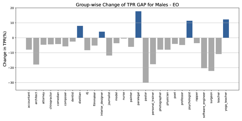
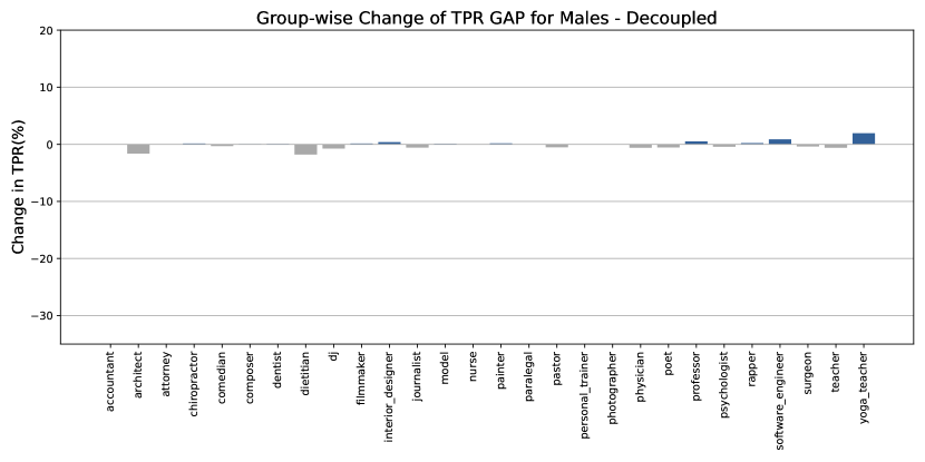
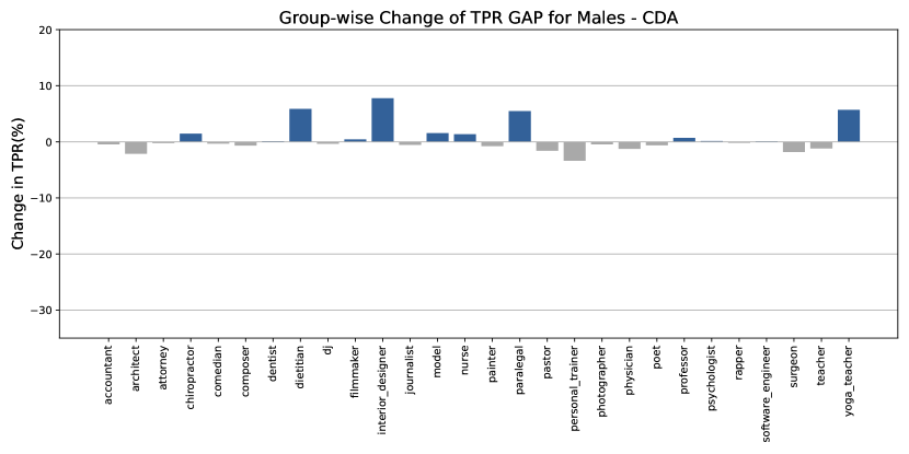
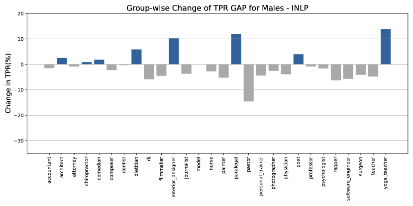
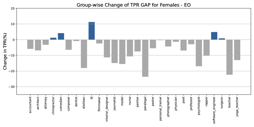
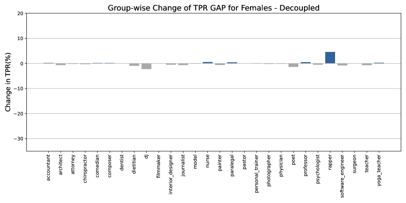
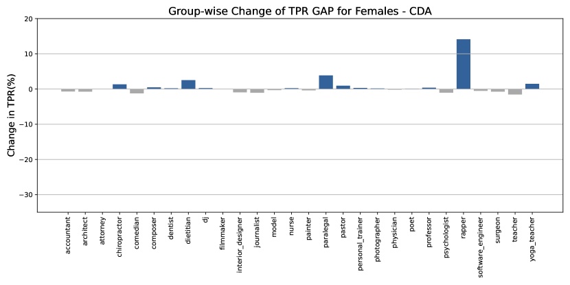
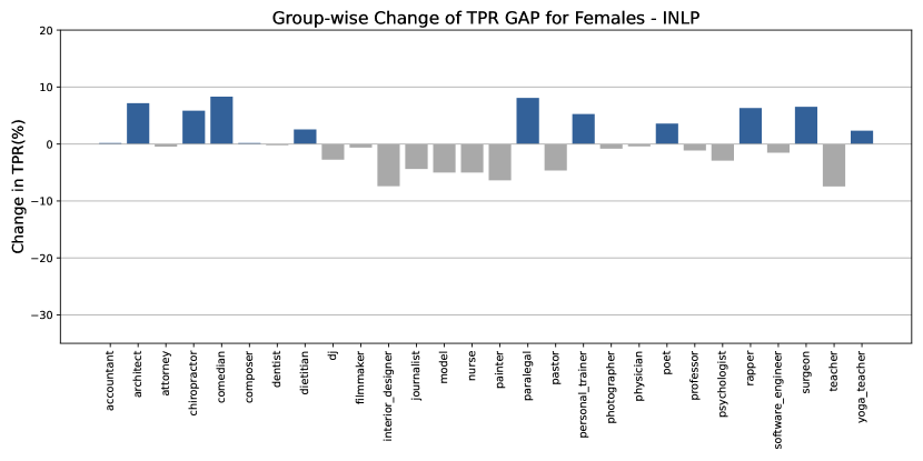
We evaluate the changes in True Positive Rate (TPR) and the changes in GAP across all professions for males and females on the debiasing techniques (Figure 6, Figure 8, Figure 10). Through the figures, we calculate the change in model performance after the debiasing and before. The blue bars denote the directions in our interest, where we want an increase in the measure of TPR and a decrease in the measure of GAP.
Appendix E Fairness with Awareness and Fairness with Unawareness
Debiasing approaches can be categorized as fairness with awareness and fairness with unawareness. Fairness with awareness refers to the approach where sensitive attributes, such as gender, race, or age, are explicitly considered in the model’s debiasing process to ensure fair outcomes [4, 28, 10]. This approach allows for targeted interventions to ensure that different demographic groups are treated equitably and has been used successfully in the fair classification literature [13]. Fairness with unawareness refers to the approach where sensitive attributes are not explicitly considered by the model [12, 9, 3]. Instead, the model is designed to ensure fair outcomes without direct knowledge of the protected attributes. This approach helps maintain privacy and limits the potential for misuse and has been the main focus of prior work on debiasing language models. Still, it may not be as effective in addressing biases rooted in complex interactions between features or when there is a strong correlation between sensitive attributes and other input features. An example of fairness with unawareness technique is adversarial debiasing [9, 3], which involves training a model to generate unbiased outputs while an adversary attempts to predict sensitive attributes from those outputs.
Appendix F Stopwords
We remove certain commonly seen words from the biography.We borrowed the list of stopwords from [20]:“i”, “me”,“my”, “myself”, “we”, “our”, “ours”, “ourselves”, “you”, “your”, “yours”, “yourself”, “yourselves”, “he”, “him”, “his”, “himself”, “she”, “her”, “hers”, “herself”, “it”, “its”, “itself”, “they”, “them”, “their”, “theirs”, “themselves”, “what”, “which”, “who”, “whom”, “this”, “that”, “these”, “those”, “am”, “is”, “are”, “was”, “were”, “be”, “been”, “being”, “have”, “has”, “had”, “having”, “do”, “does”, “did”, “doing”, “a”, “an”, “the”, “and”, “but”, “if”, “or”, “because”, “as”, “until”, “while”, “of”, “at”, “by”, “for”, “with”, “about”, “against”, “between”, “into”, “through”, “during”, “before”, “after”, “above”, “below”, “to”, “from”, “up”, “down”, “in”, “out”, “on”, “off”, “over”, “under”, “again”, “further”, “then”, “once”, “here”, “there”, “when”, “where”, “why”, “how”, “all”, “any”, “both”, “each”, “few”, “more”, “most”, “other”, “some”, “such”, “no”, “nor”, “not”, “only”, “own”, “same”, “so”, “than”, “too”, “very”, “s”, “t”, “can”, “will”, “just”, “don”, “should”, “now”