Conditional Generative Representation for
Black-Box Optimization with Implicit Constraints

Abstract

Black-box optimization (BBO) has become increasingly relevant for tackling complex decision-making problems, especially in public policy domains such as police districting. However, its broader application in public policymaking is hindered by the complexity of defining feasible regions and the high-dimensionality of decisions. This paper introduces a novel BBO framework, termed as the Conditional And Generative Black-box Optimization (CageBO). This approach leverages a conditional variational autoencoder to learn the distribution of feasible decisions, enabling a two-way mapping between the original decision space and a simplified, constraint-free latent space. The CageBO efficiently handles the implicit constraints often found in public policy applications, allowing for optimization in the latent space while evaluating objectives in the original space. We validate our method through a case study on large-scale police districting problems in Atlanta, Georgia. Our results reveal that our CageBO offers notable improvements in performance and efficiency compared to the baselines.

1 Introduction

In recent years, black-box optimization (BBO) has emerged as a critical approach in addressing complex decision-making challenges across various domains, particularly when dealing with objective functions that are difficult to analyze or explicitly define. Unlike traditional optimization methods that require gradient information or explicit mathematical formulations, black-box optimization treats the objective function as a “black box” that can be queried for function values but offers no additional information about its structure (Pardalos et al.,, 2021). This methodology is especially valuable for designing public policy, such as police districting (Zhu et al.,, 2020, 2022), site selection for emergency service systems (Xing and Hua,, 2022), hazard assessment (Xie et al.,, 2021) and public healthcare policymaking (Chandak et al.,, 2020). Policymakers and researchers in these areas frequently encounter optimization problems embedded within complex human systems, where decision evaluations are inherently implicit, and conducting them can be resource-intensive. Black-box optimization, therefore, stands out as a potent tool for navigating through these intricate decision spaces, providing a means to optimize outcomes without necessitating a detailed understanding of the underlying objective function’s analytical properties.

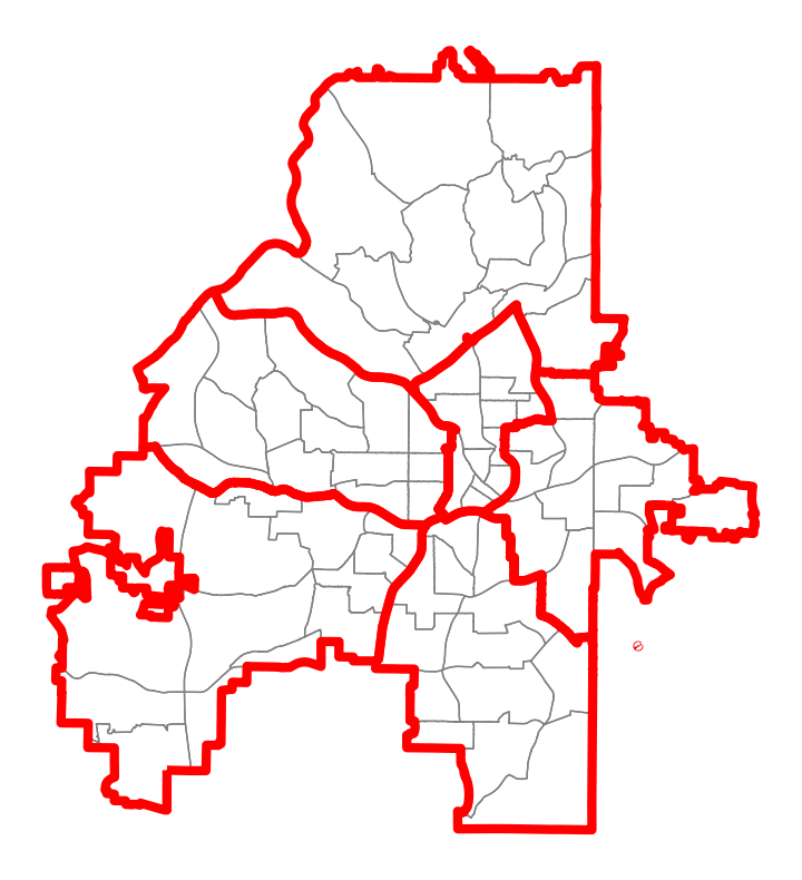
(a) Pre-2019

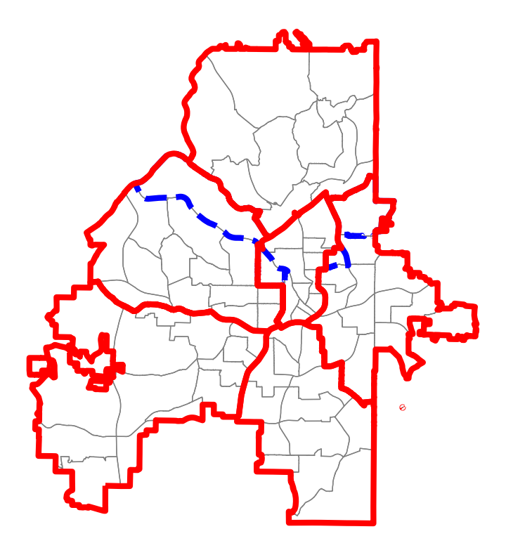
(b) Post-2019

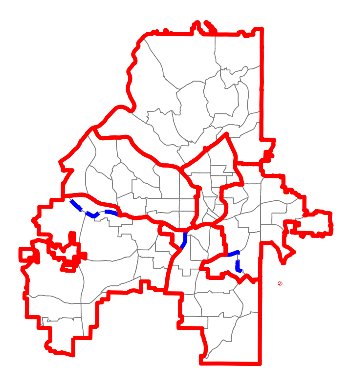
(c) Infeasible

Figure 1: An illustrative example showing the difficult-to-define constraints using three districting plans for the Atlanta Police Department (APD). Gray lines represent the basic geographical units patrolled by the police, red lines outline the districting plans, and dashed blue lines highlight the changes made to the pre-2019 plan. (a) and (b) are feasible plans implemented by the APD pre and post 2019. (c) appears to be a feasible plan but was ultimately rejected by the APD because it overlooked traffic constraints and inadvertently cut off access to some highways with its zone boundaries.

However, the broader application prospects of BBO in public policymaking are hampered due to two major hurdles: (1) Defining the feasible region or setting clear constraints for decisions is inherently complicated for real human systems. Policymakers often encounter a myriad of both explicit and implicit rules when making an optimal decision, adding a significant layer of complexity to the optimization process. For instance, in police districting, police departments often organize their patrol forces by dividing the geographical region of a city into multiple patrol areas called zones. Their goal is to search for the optimal districting plan that minimizes the workload variance across zones (Larson,, 1974; Larson and Odoni,, 1981; Zhu et al.,, 2020, 2022). As shown in Figure 1, a well-conceived plan necessitates each zone to adhere to certain shape constraints (e.g., contiguity and compactness) that are analytically challenging to formulate (Shirabe,, 2009), while also taking socio-economic or political considerations into account (e.g., ensuring fair access to public facilities). This creates a web of implicit constraints (Choi et al.,, 2000; Audet et al.,, 2020) that are elusive to define clearly and have a complex high-dimensional structure (e.g., manifold shape), making the assessment of feasible region nearly as expensive as evaluating the objective itself (Gardner et al.,, 2014). (2) The decisions for public policy are usually high-dimensional, presenting a significant computational hurdle to utilizing traditional BBO methods (Luong et al.,, 2019; Wan et al.,, 2021; Binois and Wycoff,, 2022). For example, the districting problem can be formulated by mixed-integer programming, grappling with hundreds or even thousands of decision variables even for medium-sized service systems (Zhu et al.,, 2020, 2022).

Despite the difficulty in formulating constraints for decisions in public policymaking, the rich repository of historical decisions adopted by the practitioners, combined with the increasingly easier access to human systems (van Veenstra and Kotterink,, 2017; Yu et al.,, 2021), offer a wealth of decision samples. Collecting these samples might involve seeking guidance from official public entities on decision feasibility or generating decisions grounded in domain expertise, bypassing the need to understand the explicit form of the constraints. These readily available decisions harbor implicit knowledge that adeptly captures the dynamics of implicit constraints, providing a unique opportunity to skillfully address these issues. This inspires us to develop a conditional generative representation model that maps the feasible region in the original space to a lower-dimensional latent space, which encapsulates the key pattern of these implicit constraints. As a result, the majority of existing BBO methods can be directly applied to solve the original optimization problem in this latent space without constraints.

In this paper, we aim to solve Implicit-Constrained Black-Box Optimization (ICBBO) problems. In these problems, the constraints are not analytically defined, however the feasibility of a given decision can be easily verified. We introduce a new approach called Conditional And Generative Black-box Optimization (CageBO). Using a set of labeled decisions as feasible or infeasible, we first construct a conditional generative representation model based on the conditional variational autoencoder (CVAE) (Sohn et al.,, 2015) to explore and generate new feasible decisions within the intricate feasible region. To mitigate the impact of potentially poorly generated decisions, we adopt a post-decoding process that aligns these decisions closer to the nearest feasible ones. Furthermore, we incorporate this conditional generative representation model as an additional surrogate into our black-box optimization algorithm, allowing for a two-way mapping between the feasible region in the original space and an unconstrained latent space. As a result, while objective function is evaluated in the original space, the black box optimization algorithm is performed in the latent space without constraints. We prove that our proposed algorithm can achieve a no-regret upper bound with a judiciously chosen number of observations in the original space. Finally, we validate our approach with numerical experiments on both synthetic and real-world datasets, including applying our method to address large-scale districting challenges within police operation systems in Atlanta, Georgia, demonstrating its significant empirical performance and efficiency over existing methods.

Contributions. Our contributions are summarized as:

1. We formulate a novel class of optimization problems called Implicit Constrained Black-Box Optimization (ICBBO) and develop the CageBO algorithm that effectively tackles high-dimensional ICBBO problems.

2. We introduce a conditional generative representation model that constructs a lower-dimensional, constraint-free latent space. This space enables BBO algorithms to efficiently search and generate new feasible candidate solutions.

3. By proving the no-regret expected cumulative regret bound, we show that our CageBO algorithm is able to find the global optimal solution.

4. Our empirical results demonstrate the superior performance of our model against the baseline methods on both synthetic and real data sets, particularly in scenarios with complex implicit constraints.

Related work. Black-box optimization, a.k.a. zeroth-order optimization or derivative-free optimization, is a long-standing challenging problem in optimization and machine learning. Existing work either assumes the underlying objective function is drawn from some Gaussian process (Williams and Rasmussen,, 2006) or some parametric function class (Dai et al.,, 2022; Liu and Wang,, 2023). The former one is usually known as Bayesian optimization (BO), with the Gaussian process serving as the predominant surrogate model. BO has been widely used in many applications, including but not limited to neural network hyperparameter tuning (Kandasamy et al.,, 2020; Turner et al.,, 2021), material design (Ueno et al.,, 2016; Zhang et al.,, 2020), chemical reactions (Guo et al.,, 2023), and public policy (Xing and Hua,, 2022).

In numerous real-world problems, optimization is subject to various types of constraints. Eriksson proposes scalable BO with known constraints in high dimensions (Eriksson and Poloczek,, 2021). Letham explores BO in experiments featuring noisy constraints (Letham et al.,, 2019). Gelbart pioneered the concept of BO with unknown constraints (Gelbart et al.,, 2014), later enhanced by Aria through the ADMM framework (Ariafar et al.,, 2019). Their constraints are unknown due to uncertainty but can be evaluated using probabilistic models. In addition, Choi and Audet study the unrelaxable hidden constraints in a similar way (Choi et al.,, 2000; Audet et al.,, 2020), where the feasibility of a decision can be evaluated by another black-box function. In contrast, the implicit constraints are unknown due to the lack of analytical formulations in our problem.

Building on latent space methodologies, Varol presented a constrained latent variable model integrating prior knowledge (Varol et al.,, 2012). Eissman (Eissman et al.,, 2018) presents a VAE-guided Bayesian optimization algorithm with attribute adjustment. Deshwal and Doppa focus on combining latent space and structured kernels over combinatorial spaces (Deshwal and Doppa,, 2021). Maus further investigates structured inputs in local spaces (Maus et al.,, 2022), and Antonova introduces dynamic compression within variational contexts (Antonova et al.,, 2020). However, it’s worth noting that none of these studies consider any types of constraints in their methodologies.

Additionally, there is another line of work aiming to solve offline black-box optimization. Notable contributions in this domain include the works of Char and Chen, who focus on leveraging offline contextual data for optimization (Char et al.,, 2019; Chen et al.,, 2023), and Krishnamoorthy, who delves into offline black-box optimization via diffusion models (Krishnamoorthy et al.,, 2023). Similar to our approach, these studies adopt data-driven methodologies but in an offline manner, which limits their applicability in the dynamic and evolving field of public policymaking.

2 Preliminaries

Problem setup. We consider a decision space denoted by $\mathcal{X}\subseteq[0,1]^{d}$ where $1$ can be replaced with any universal constant w.l.o.g., which represents a specific region of a $d$-dimensional real space. Suppose there exists a black-box objective function, $f:\mathcal{X}\mapsto\mathbb{R}$, that can be evaluated, albeit at a substantial cost. Assume we can obtain a noisy observation of $f(x)$, denoted as $\hat{f}(x)=f(x)+\epsilon$, where $\epsilon$ follows a $\sigma$-sub-Gaussian noise distribution. The goal is to solve the following optimization problem:

$$\min_{x\in\mathcal{X}}~{} f(x),$$ (1)

s.t. $$x\in\mathcal{S},$$ (2)

where $\mathcal{S}\subseteq\mathcal{X}$ represents the feasible region, defined by a set of implicit constraints.

Given the analytical expressions of the implicit constraints are not directly accessible, explicitly formulating these constraints is not feasible. However, they can still be evaluated through a feasibility oracle $h(\cdot):\mathcal{X}\mapsto\{0,1\}$, where a value of 1 indicates feasible, and 0 indicates infeasible. Now suppose we have access to a human system that provides labeled decisions. Denote a set of labeled decisions by $\mathcal{D}=\{(x_{i},c_{i})\},i\in[n]$, where $x_{i}\in\mathcal{X}$ represents the $i$th decision and $c_{i}\in\{0,1\}$ represents its feasibility. Assume $\mathcal{D}$ has a good coverage of the decision space of interest. In practice, decisions can be derived from consultations within human systems or crafted using domain expertise, with the feasibility oracle effectively acting as a surrogate for a policymaker. For example, new feasible districting plans in Figure 1 can be created by first randomly altering the assignments of border regions and then checking their feasibility through police consultations.

Bayesian optimization. The BO algorithms prove especially valuable in scenarios where the evaluation of the objective function is costly or time-consuming, or when the gradient is unavailable. This approach revolves around constructing a surrogate model of the objective function and subsequently employing an acquisition function based on this surrogate model to determine the next solution for evaluation. For the minimization problem, a popular choice of surrogate model is the Gaussian process with the lower confidence bound (LCB) (Srinivas et al.,, 2009) serving as the acquisition function.

The Gaussian process (GP) in the space $\mathcal{X}$, denoted by $\text{GP}({\mu},{k};\mathcal{X})$, is specified by a mean function ${\mu(x)}$ and a kernel function $k(x,x^{\prime})$, which indicates the covariance between the two arbitrary decisions $x$ and $x^{\prime}$. The GP captures the joint distribution of all the evaluated decisions and their observed objective function values. We reference the standard normal distribution with zero mean and an identity matrix $I$ as its variance by $\mathcal{N}(0,I)$, and let $Y=\{\hat{f}(x)\mid x\in X\}$ represent the corresponding set of objective function values. For a new decision $\tilde{x}$, the joint distribution of $Y$ and its objective function value $\tilde{y}$ of $\tilde{x}$ is

$$\begin{bmatrix}Y\\ \tilde{y}\end{bmatrix}\sim\mathcal{N}\left(\mu\left(\begin{bmatrix}X\\ \tilde{x}\end{bmatrix}\right),\begin{bmatrix}K(X,X)+\sigma^{2}I&K(X,\tilde{x})\\ K(X,\tilde{x})^{\top}&k(\tilde{x},\tilde{x})\end{bmatrix}\right),$$

where $\sigma^{2}$ represent the variance of the observed noise $\epsilon$. Here $K(X,X)=\left(k\left(x,x^{\prime}\right)\right)_{x,x^{\prime}\in\mathcal{X}}$ denotes the covariance matrix between the previously evaluated decisions and $K(X,\tilde{x})=\left(k\left(x,\tilde{x}\right)\right)_{x\in\mathcal{X}}$ denotes the covariance vector between the previously evaluated and the new decisions.

3 Proposed method

The main idea of our method is to perform Bayesian optimization within a low-dimensional latent space denoted as $\mathcal{Z}\subseteq\mathbb{R}^{d^{\prime}}$ with $d^{\prime}\ll d$, rather than the constrained original decision space. The latent space $\mathcal{Z}$ is learned using a CVAE, which leverages the set of labeled decisions $\mathcal{D}$ as the training data.

To be specific, we train the CVAE model by maximizing $\mathcal{L}_{\mathrm{ELBO}}$ on the training data $\mathcal{D}$. This CVAE model enables a two-way mapping of decisions between the original and latent spaces, through an encoder_ϕ from the learned conditional distribution $q_{\phi}(z|x,c)$ and a decoder_θ from the learned conditional posterior $p_{\theta}(x|z,c)$. Given an initial set of decisions $X_{0}$ randomly sampled from the feasible set $\mathcal{D}_{f}$, we first evaluate their objective values denoted as $Y_{0}=\{\hat{f}(x)\mid x\in X_{0}\}$. These decisions are then encoded to the latent space, represented by $Z_{0}\subset\mathcal{Z}$. As illustrated by Figure 2, for each iteration $t$, our BO algorithm is performed as follows: (1) Train a surrogate model $\text{GP}(\mu,k;\mathcal{Z})$ using the current latent decisions $Z_{t-1}$ and their observed values $Y_{t-1}$. (2) Identify the next latent decision candidate $z_{t}$ by searching on the feasible latent space $\hat{Z}$, defined as the support of the latent variable distribution conditioned on feasibility $c=1$, and select the one exhibiting the lowest LCB value. (3) Decode the latent decision candidate $z_{t}$ to the original space, yielding a new decision ${x}_{t}$. (4) Assess the feasibility of ${x}_{t}$ via the feasibility oracle $h$. If ${x}_{t}$ is feasible, evaluate its objective value and include it in the feasible set $\mathcal{D}_{f}$. Otherwise, apply the post-decoding process $\psi_{\mathcal{D}_{f}}$ before evaluating the objective value. (5) Update the observations $Z_{t}$ and $Y_{t}$ accordingly. The CageBO algorithm iterates a total of $T$ times. The proposed method is summarized in Algorithm 1. In the remainder of this section, we explain each component of our proposed method at length.

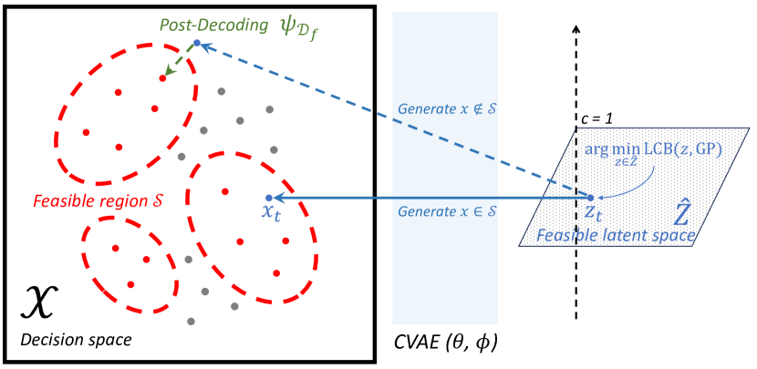
Figure 2: An illustration of the CageBO algorithm. Red dots represent observed feasible decisions, and grey dots denote observed infeasible decisions. The red dotted circle illustrates the complex feasible region that is not directly accessible. For each iteration, a new decision $z_{t}$ is then chosen in the feasible latent space $\hat{Z}$ by minimizing the lower confidence bound (LCB). This new decision $z_{t}$ is mapped back to the original space as $x_{t}$ using ${\mathrm{decoder}}_{\theta}$. If the CVAE model is well-trained, the newly generated $x_{t}$ is highly likely to reside within the feasible set $\mathcal{S}$. In case $x_{t}\notin\mathcal{S}$, the post-decoding process $\psi_{\mathcal{D}_{f}}$ will adjust it to the nearest observed feasible decision.

3.1 Conditional generative representation

To address the challenge of implicit constraints in ICBBO problems, we introduce a conditional generative representation model based on a CVAE in our framework. The rationale behind our approach is threefold: (1) To encode the original decision space with implicit constraints into a compact, continuous, and constraint-free latent space. (2) To condense the dimensionality of the original problem, making BBO more efficient in the latent space. (3) To actively search for solutions with a high likelihood of being feasible. As illustrated by Figure 3, we observe that BBO can navigate within a feasible latent space, which offers a simpler structure in the objective function, facilitated by the conditional generative representation model.

Algorithm 1 CageBO

  Input: Labeled decisions $\mathcal{D}$; Objective function $\hat{f}$; Feasibility oracle $h$; Hyper-parameters $T$.

  Train a CVAE$(p_{\theta},q_{\phi})$ by maximizing $\mathcal{L}_{\mathrm{ELBO}}$ in $\mathcal{D}$;

  Feasible set $\mathcal{D}_{f}=\{x_{i}\in\mathcal{X}\mid(x_{i},c_{i})\in\mathcal{D}\text{ and }c_{i}=1\}$;

  Initialize $X_{0}\subseteq\mathcal{D}_{f}$, $Y_{0}=\{\hat{f}({x})\mid{x}\in X_{0}\}$; $Z_{0}\leftarrow{\mathrm{encoder}}_{\phi}(X_{0})$; // Encoding

  for $t=1\textbf{ to }T$ do

     Train $\text{GP}(\mu,k;\mathcal{Z})$ using $(Z_{t-1},Y_{t-1})$;

     $\hat{Z}=\mathrm{supp}(q_{\phi}(\cdot|c=1))$;

     ${z}_{t}\in\mathop{\mathrm{argmin}}_{z\in\hat{Z}}\operatorname{LCB}\left(z,\text{GP}\right)$;

     ${x_{t}}\leftarrow{\mathrm{decoder}}_{\theta}({z}_{t})$; // Decoding

     if $h(x_{t})=1$ then

        $y_{t}=\hat{f}({x}_{t})$, $\mathcal{D}_{f}\leftarrow\mathcal{D}_{f}\cup\{x_{t}\}$;

     else

        $y_{t}=\hat{f}(\psi_{\mathcal{D}_{f}}({x_{t}}))$; // Post-decoding

     end if

     $Z_{t}\leftarrow Z_{t-1}\cup\{z_{t}\}$, $Y_{t}\leftarrow Y_{t-1}\cup\{y_{t}\}$;

  end forreturn $x^{*}\in\text{argmin}_{{x}\in X_{T}}\hat{f}({x})$

Suppose there exists a joint distribution between the decision variable $x\in\mathcal{X}\subseteq\mathbb{R}^{d}$ and a latent variable $z\in\mathcal{Z}\subseteq\mathbb{R}^{d^{\prime}}$, conditioned on the feasibility criterion $c$, with $d^{\prime}\ll d$. We model the conditional distributions $q_{\phi}(z|x,c)$, $p_{\theta}(x|z,c)$, and the conditional prior $p(z|c)$ through the use of neural networks as outlined in (Pinheiro Cinelli et al.,, 2021). Here, $\phi$ and $\theta$ represent the neural network weights associated with each respective distribution. Since it is intractable to directly optimize the marginal maximum likelihood of $x$, the evidence lower bound (ELBO) (Jordan et al.,, 1999) of the log-likelihood is derived as follows

$$\begin{split}\mathcal{L}_{\mathrm{ELBO}}&=w(c)\underset{q_{\phi}(z|x,c)}{\mathbb{E}}\left[\log p_{\theta}(x|z,c)\right]\\ &\quad-\eta\mathrm{D}_{\mathrm{KL}}\left(q_{\phi}(z|x,c)\|p(z|c)\right),\end{split}$$ (3)

where $w(c)$ denotes the weighting function associated with the feasibility $c$, and $\eta$ is a hyperparameter controlling the penalty ratio. Here we assume the conditional prior of $z$ follows a standard Gaussian distribution $\mathcal{N}(0,I)$. The first term in (3) can be considered as the reconstruction error between the input and reconstructed decisions, and the second term is the Kullback–Leibler (KL) divergence between the conditional prior of the latent variable $z$ and the learned posterior $q_{\phi}(z|x,c)$.

Post-decoding process. To ensure the decoded decision ${x}\in\mathcal{X}$ is subject to the implicit constraints, we introduce a post-decoding process in addition to the decoder, denoted by $\psi_{\mathcal{S}}:\mathcal{X}\mapsto\mathcal{S}$. This function projects any given decision ${x}\in\mathcal{X}$ to the closest feasible decision $\hat{x}\in\mathcal{S}$. However, the presence of implicit constraints prevents us from achieving an exact projection. As a workaround, we search within the observed feasible set $\mathcal{D}_{f}=\{x_{i}\in\mathcal{X}\mid(x_{i},c_{i})\in\mathcal{D}\text{ and }c_{i}=1\}$, rather than the unattainable feasible region $\mathcal{S}$, and find a feasible decision $\hat{x}\in D_{f}$ that is the closest to the decoded decision ${x}$ as an approximate. The distance between any two decisions is measured by the Euclidean norm $||\cdot||_{2}$. Formally,

$$\psi_{\mathcal{D}_{f}}({x})=\mathop{\mathrm{argmin}}_{\hat{x}\in\mathcal{D}_{f}}||\hat{x}-x||_{2}.$$ (4)

The post-decoding process is initiated only for decoder-generated decisions $x$ that are infeasible. Feasible decisions are directly incorporated into the observed feasible set $\mathcal{D}_{f}$. Through iteratively expanding this observed feasible set, we enhance the accuracy of this process by improving the coverage of $\mathcal{D}_{f}$ on the underlying feasible region $\mathcal{S}$.

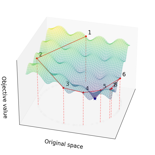
(a) Original space

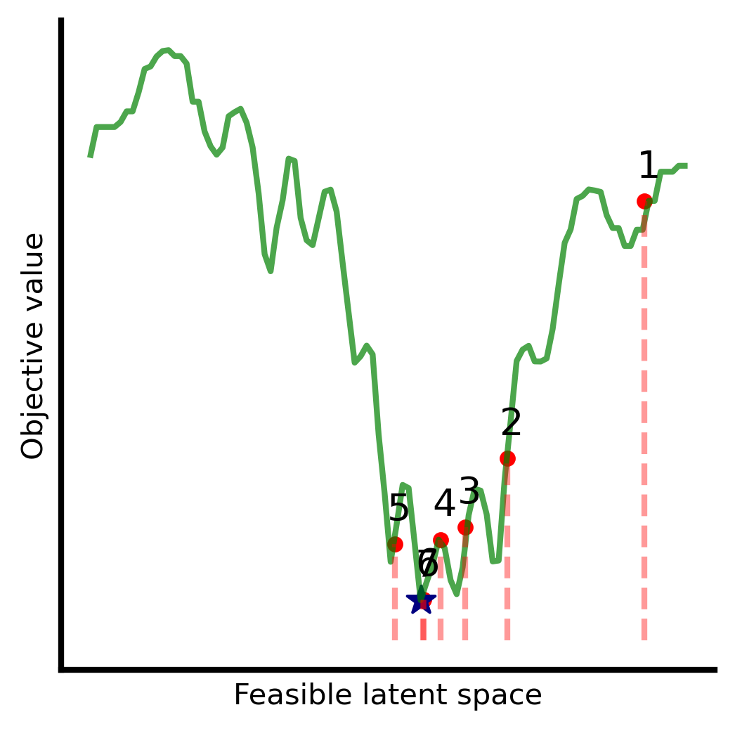
(b) Feasible latent space

Figure 3: Solution paths of the same optimization problem suggested by our CageBO algorithm in the (a) original and (b) latent spaces, respectively. The objective in this illustrative example is to minimize the Ackley function subject to an “implicit” constraint (a circle) in a 2-dimensional decision space.

3.2 Surrogate model

Now we define an indirect objective function $g(\cdot)$ which maps from $\mathcal{Z}\mapsto\mathbb{R}$:

$$g(z)=\begin{cases}f({\mathrm{decoder}}_{\theta}(z)),&\text{if }h({\mathrm{decoder}}_{\theta}(z))=1,\\ f(\psi_{\mathcal{D}_{f}}({\mathrm{decoder}}_{\theta}(z))),&\text{if }h({\mathrm{decoder}}_{\theta}(z))=0.\end{cases}$$

The indirect objective function measures the objective value of the latent variable via the decoding and the potential post-decoding process. Given that the objective function $f$ is inherently a black-box function, it follows that the indirect objective function $g$ is also a black-box function.

We use a GP as our surrogate model of the indirect objective function $g$, denoted by $\text{GP}({\mu},{k};\mathcal{Z})$. In our problem, the mean function can be written as ${\mu(z)=\mathbb{E}[g(z)]}$. In addition, we adopt the Matérn kernel (Seeger,, 2004) as the kernel function $k(z,z^{\prime})=\mathbb{E}[(g(z)-\mu(z))(g(z^{\prime})-\mu(z^{\prime}))]$, which is widely-used in BO literature. The main advantage of the GP as a surrogate model is that it can produce estimates of the mean evaluation and variance of a new latent variable, which can be used to model uncertainty and confidence levels for the acquisition function described in the following. Note that the latent variable $z$ is assumed to follow a Gaussian prior in the latent decision model, which aligns with the assumption of the GP model that the observed latent variables $Z$ follow the multivariate Gaussian distribution.

Acquisition function. In the BO methods, the acquisition function is used to suggest the next evaluating candidate. Our approach adopts the lower confidence bound (LCB) as the acquisition function to choose the next latent variable $z$ candidate to be decoded and evaluated. This function contains both the mean $\mu(z)$ of the GP as the explicit exploitation term and the standard deviation $\sigma(z)$ of the GP as the exploration term:

$$\mathrm{LCB}(z,\text{GP})=\mu(z)-\sqrt{\beta}\sigma(z),$$ (5)

where $\beta$ is a trade-off parameter.

To identify new latent decisions for evaluation, our method draws numerous independent samples from the conditional posterior $q_{\phi}(\cdot|x,c=1)$ among observed feasible decisions $x\in\mathcal{D}_{f}$. The sample with the lowest LCB value, denoted as $z_{t}$, is selected for decoding and subsequent evaluation using the objective function $\hat{f}$ in the $t$-th iteration.

3.3 Theoretical analysis

We provide theoretical analysis for Algorithm 1. Let $\mathtt{enc}:\mathcal{X}\mapsto\mathcal{Z}$ denote the encoder function, $\mathtt{dec}:\mathcal{Z}\mapsto\mathcal{X}$ denote the decoder function, and $g(z)=f(\psi_{\mathcal{D}_{f}}(\mathtt{dec}(z))):\mathcal{Z}\mapsto\mathbbm{R}$ denotes the objective function w.r.t. $\mathcal{Z}$ where $\psi_{\mathcal{D}_{f}}$ is the post-decoder. Note even if post-decoder is not needed, $\psi_{\mathcal{D}_{f}}(\mathtt{dec}(z))=\mathtt{dec}(z)$. Following the existing work in Gaussian process bandit optimization, we utilize cumulative regret and its expected version to evaluate the performance of our algorithm which are defined as follows.

$$R_{T} =\sum_{i=1}^{T}f(x_{t})-f(x_{*}),$$ (6)

$$\mathbb{E}[R_{T}] =\mathbb{E}\left[\sum_{i=1}^{T}f(x_{t})-f(x_{*})\right],$$ (7)

where $x_{*}=\mathop{\mathrm{argmax}}_{x\in\mathcal{X}}f(x)$ and the expectation is taken over all randomness, including random noise and random sampling over observations.

We assume the distance between any two points in $\mathcal{Z}$ can be upper bounded by their distance in $\mathcal{X}$, i.e., $\forall x,x^{\prime}\in\mathcal{X},\|\mathtt{enc}(x)-\mathtt{enc}(x^{\prime})\|_{2}\leq C_{p}\|x-x^{\prime}\|_{2}$. We further assume that function $g:\mathcal{Z}\mapsto\mathbbm{R}$ is drawn from a Gaussian Process prior and it is $C_{g}$-Lipschitz continuous, i.e., $\forall z,z^{\prime}\in\mathcal{Z},|g(z)-g(z^{\prime})|\leq C_{g}\|z-z^{\prime}\|_{2}$. Now we are ready to state our main theoretical result.

Theorem 1.

After running $T$ iterations, the expected cumulative regret of Algorithm 1 satisfies that

$$\mathbb{E}[R_{T}]=\widetilde{O}(\sqrt{T\gamma_{T}}+\sqrt{d}(n+T)^{\frac{d}{d+1}}),$$ (8)

where $\gamma_{T}$ is the maximum information gain, depending on choice of kernel used in algorithm and $n$ is number of initial observation data points.

Remark 2.

We present an upper bound of expected cumulative regret of our Algorithm 1. This is a no-regret algorithm since $\lim_{T\rightarrow\infty}\mathbb{E}[R_{T}]/T=0$ which means our algorithm is able to find the global optimal solution by expectation. The bound has two terms. The first term follows from GP-UCB (Srinivas et al.,, 2010) where the maximum information gain depends on the choice of kernel used in the algorithm. For linear kernel, $\gamma_{T}=O(d\log T)$ and for squared exponential kernel, $\gamma_{T}=O(\log T)^{d+1}$. The second term is the regret term incurred by the post decoder $\psi_{\mathcal{D}_{f}}$, which is also sublinear in $T$ if $n$ is chosen no larger than $T$.

Technical lemmas. Our proof relies on the following two lemmas and full proof is shown in Appendix A.

Lemma 3 (Regret bound of GP-LCB (Theorem 1 of (Srinivas et al.,, 2010))).

Let $\delta\in(0,1)$ and $\beta_{t}=2\log(mt^{2}\pi^{2}/6\delta)$. Running GP-UCB with $\beta_{t}$ for a sample $f$ of a GP with mean function zero and covariance function $k(x,x^{\prime})$, we obtain a regret bound of $\widetilde{O}(\sqrt{T\gamma_{T}\log n})$ with high probability. Precisely,

$$\mathbb{P}[R_{T}\geq\sqrt{C_{1}T\beta_{T}\gamma_{T}}\ \forall T\geq 1]\geq 1-\delta,$$ (9)

where $C_{1}=8/\log(1+\delta^{-2})$.

Lemma 4 (Expected minimum distance (Lemma 19.2 of (Shalev-Shwartz and Ben-David,, 2014))).

Let $C_{1},...,C_{r}$ be a collection of covering sets of some domain set $\mathcal{X}$. Let $S$ be a sequence of $n$ points sampled i.i.d. according to some probability distribution $\mathcal{D}$ over $\mathcal{X}$. Then,

$$\mathbb{E}_{S\sim\mathcal{D}^{n}}\left[\sum_{i\in C_{i}\cap S=\emptyset}\mathbb{P}(C_{i})\right]\leq\frac{r}{ne}.$$ (10)

4 Experiments

4.1 Experimental setup

We compare our CageBO algorithm against three baseline approaches that can be used to address ICBBO problems. These baselines include (1) simulated annealing (SA) (Kirkpatrick et al.,, 1983) (details in Appendix C), (2) approximated Mixed Integer Linear Programming (MILP) (Zhu et al.,, 2022), and (3) a VAE-guided Bayesian optimization algorithm (VAE-BO) (Eissman et al.,, 2018) that only trained on the feasible data. We train the latent decision model in our framework with the Adam optimizer (Kingma and Ba,, 2015). Both CageBO and VAE-BO are trained and performed under an identical environment. Each method is executed 10 times across all experiments to determine the $95\%$ confidence interval of their results.

Experiments were conducted on a PC equipped with M1 Pro CPU and 16 GB RAM. For synthetic experiments, CageBO is trained in $1,000$ epoches with the learning rate of $10^{-4}$, $w(1)=2$, $w(0)=1$, $\eta=0.1$, and dimension of latent space $d^{\prime}=10$. Hyperparameters: $|X_{0}|=10$ initial evaluation points, $\beta=1$ for the LCB, and $T=100$. For real-world redistricting experiments, CageBO is trained in $1,000$ epoches with the learning rate of $10^{-4}$, $w(1)=2$, $w(0)=1$, $\eta=0.1$, and dimension of latent space $d^{\prime}=25$. Hyperparameters: $|X_{0}|=5$ initial evaluation points, $\beta=1$ for the LCB, $T=50$ ($6\times 6$ grid) and $T=100$ (Atlanta).

Note that we only include MILP as a baseline method in the districting problems because the continuity and compactness in these problems can be expressed as a set of linear constraints, albeit with the trade-offs of adding auxiliary variables and incurring computational expenses. Nonetheless, in other scenarios, including our synthetic experiments, direct application of MILP is not feasible.

4.2 Synthetic results

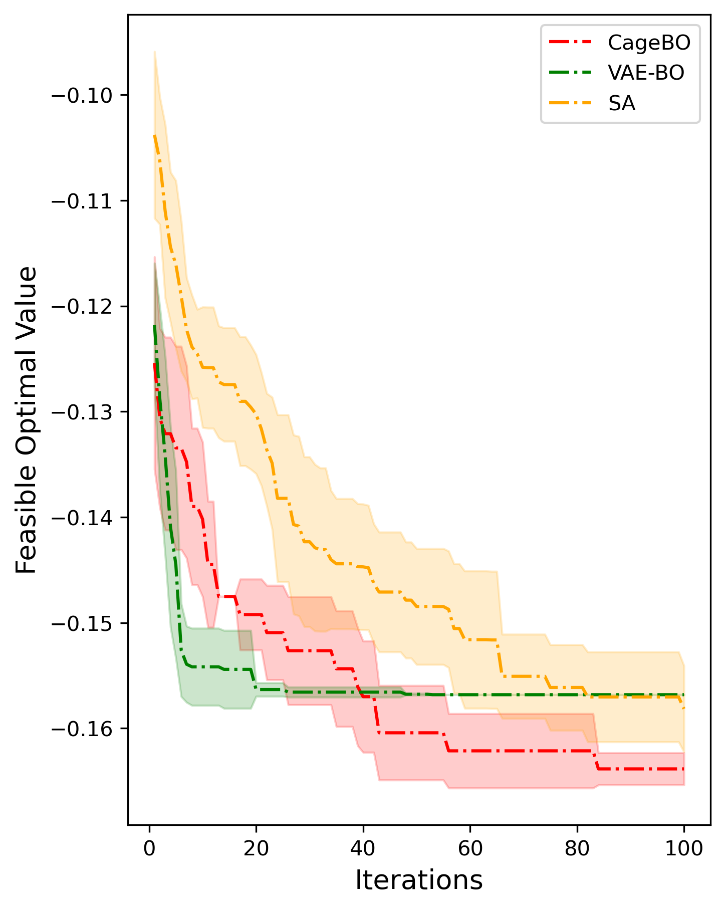
(a) Keane’s bump function

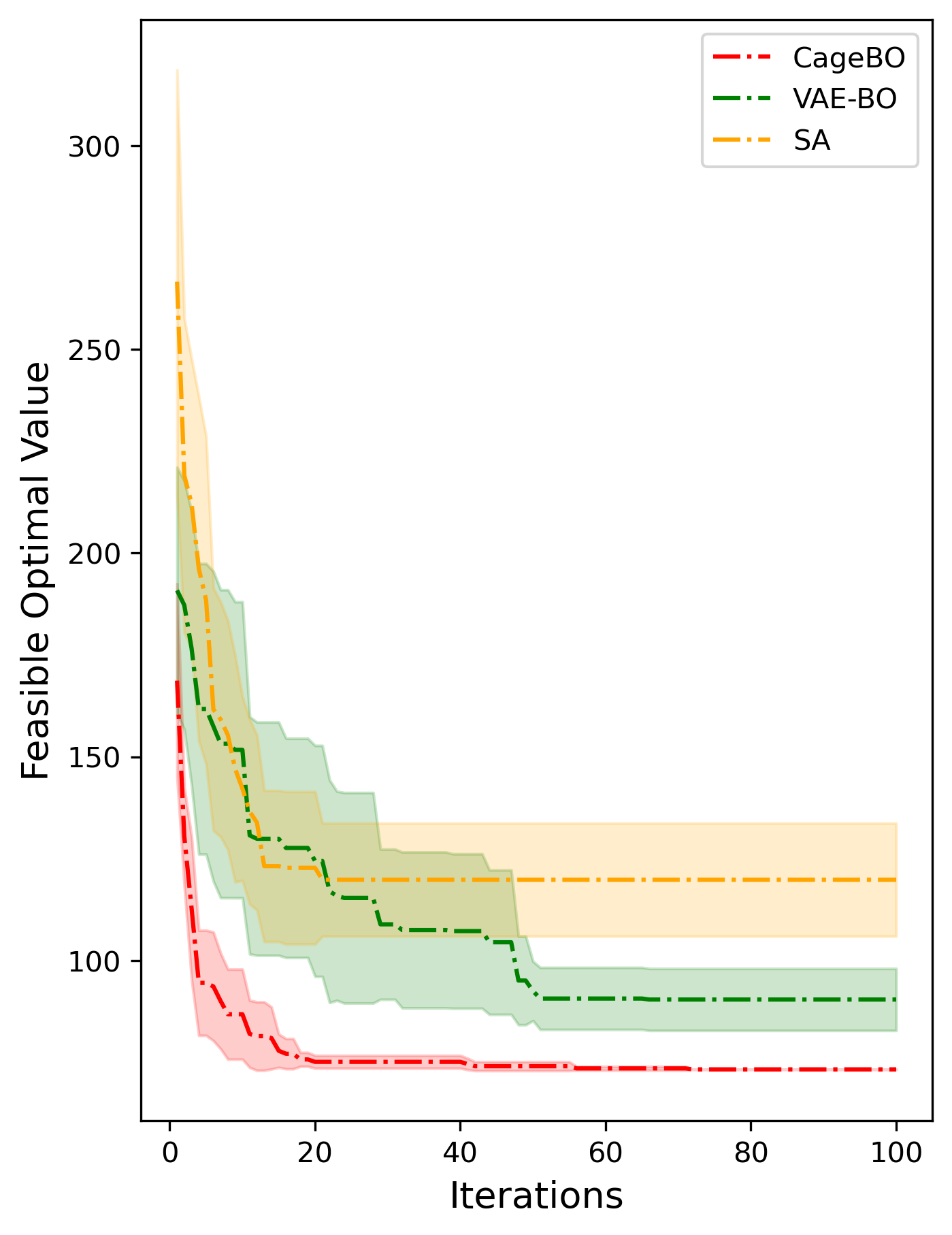
(b) Levy function

Figure 4: Comparisons of performance convergence with 95% confidence intervals for (a) 30-dimensional Keane’s bump function and (b) 50-dimensional Levy function, respectively.

We consider minimizing (a) the $30$D Keane’s bump function (Keane,, 1994) and (b) the $50$D Levy function (Laguna and Martí,, 2005), both of which are common test functions for constrained optimization. To obtain samples from implicit constraints, the conundrum we aim to address via our methodology, we first generate $n=2,000$ samples from the standard uniform distribution in the $10$-dimensional latent space, then decode half of them through a randomly initialized decoder and mark those as feasible. We define the feasibility oracle to return 1 only if the input solution is matched with a feasible solution. We scale the samples accordingly so that the test functions can be evaluated under their standard domains, i.e., the Keane’s bump function on $[0,10]^{d}$ and the Levy function on $[-10,10]^{d}$.

Figure 4 presents the synthetic results. It is evident that our method attains the lowest objective values consistently compared to other baseline methods. In Figure 4 (b), in particular, we observe that the integration of the conditional generative representation model into CageBO greatly enhances the BO’s performance. This is in stark contrast to VAE-BO and SA, which don’t yield satisfactory outcomes.

4.3 Case study: Police redistricting

One common application of high-dimensional ICBBO in public policymaking is redistricting. For example, in police redistricting problems, the goal is to distribute $L$ police service regions across $J$ distinct zones. Each service region is patrolled by a single police unit. While units within the same zone can assist each other, assistance across different zones is disallowed. The decision variables are defined by the assignment of a region to a zone, represented by matrix $x\in\{0,1\}^{L\times J}$. Here, an entry $x_{lj}=1$ indicates region $l$ is allocated to zone $j$, and $x_{lj}=0$ otherwise. A primal constraint is that each region should be assigned to only one zone. This means that for every region $l$, $\sum_{j\in[J]}x_{lj}=1$. The implicit constraint to consider is the contiguity constraint, which ensures that all regions within a specific zone are adjacent. We define the feasibility oracle to return 1 only if both the primal and the implicit constraint are satisfied.

The objective of the police redistricting problem is to minimize the workload variance across all the districts. The workload for each district $j$, denoted as $\rho_{j}$, is computed using the following equation:

$$\rho_{j}=({\tau}_{j}+1/\mu)\lambda_{j}.$$ (11)

In this equation, ${\tau}_{j}$ represents the average travel time within district $j$, which can be estimated using the hypercube queuing model (Larson,, 1974), which can be regarded as a costly black-box function. Assuming $\mu$ represents the uniform service rate across all districts and $\lambda_{j}$ denotes the arrival rate in district $j$. Essentially, $\rho_{j}$ quantifies the cumulative working duration per unit time for police units in district $j$. For clarity, a value of $\rho_{j}=10$ implies that the combined working time of all police units in district $j$ counts to 10 hours or minutes in every given hour or minute.

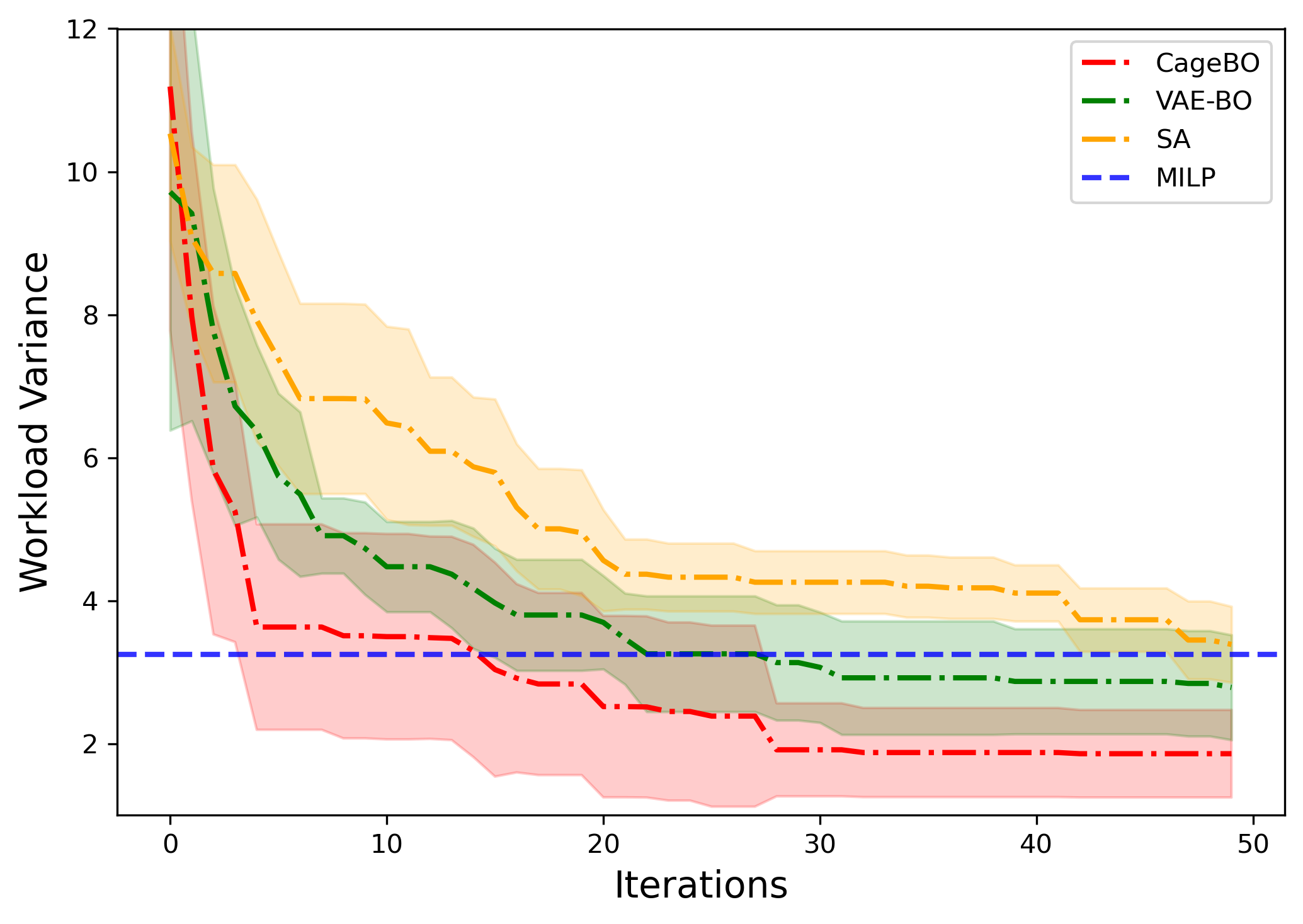
Figure 5: Performance convergence with a 95% confidence interval on the $6\times 6$ grid districting problem.

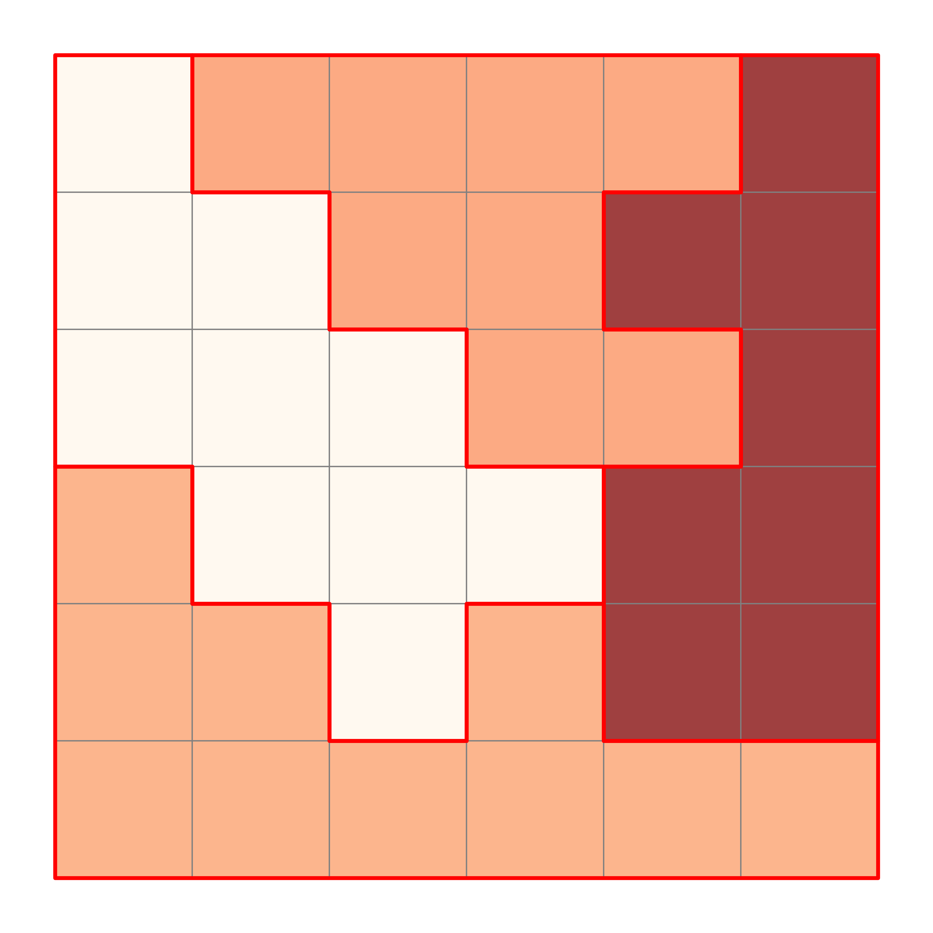
(a) MILP

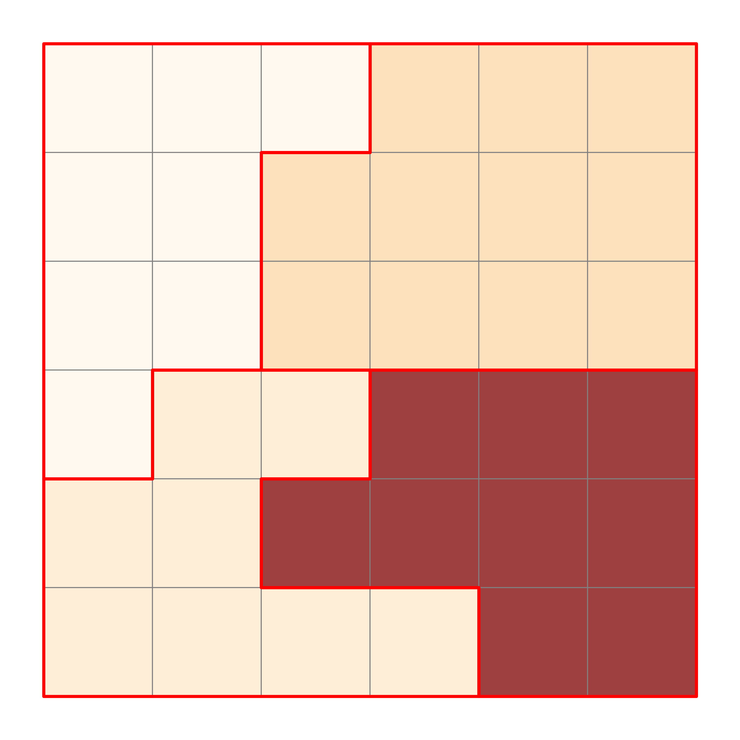
(b) SA

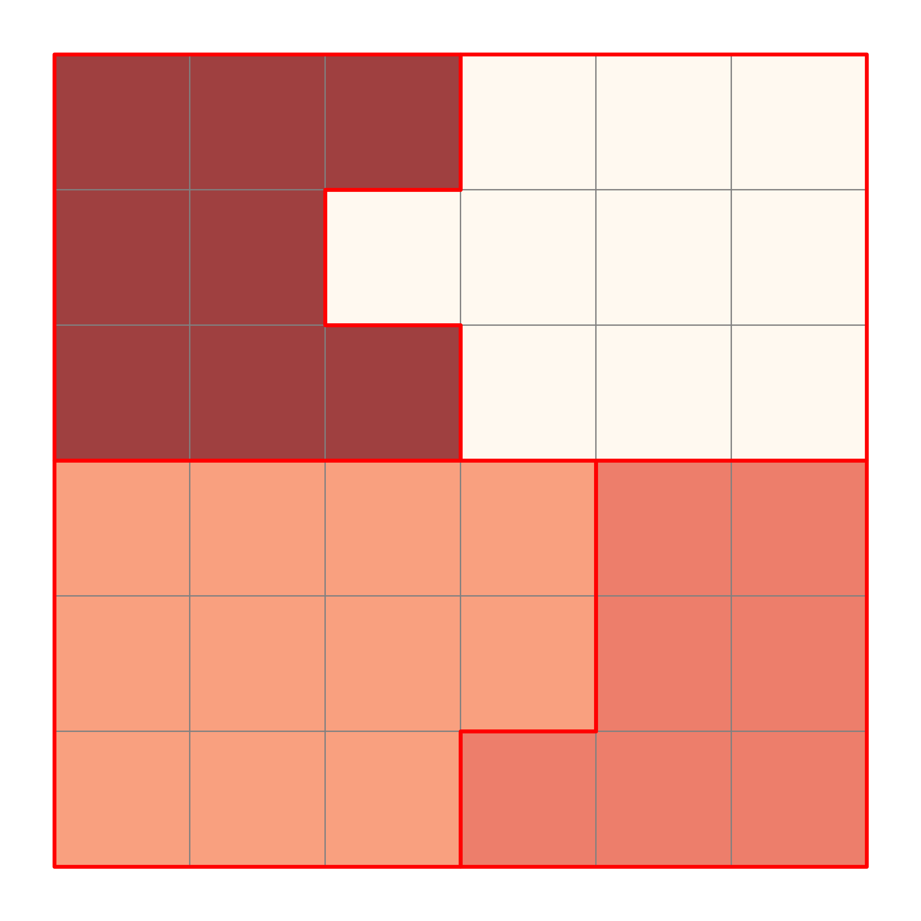
(c) VAE-BO

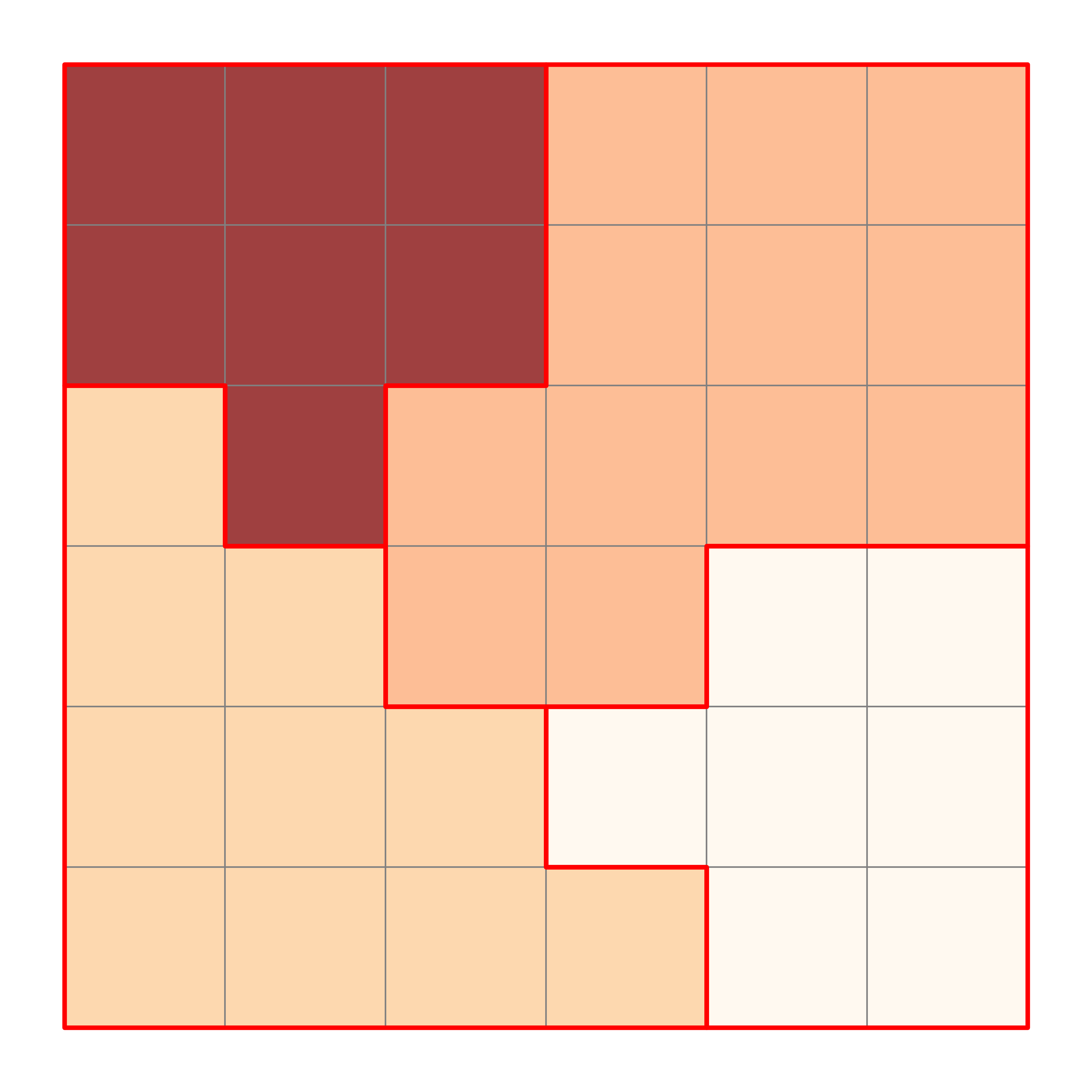
(d) CageBO

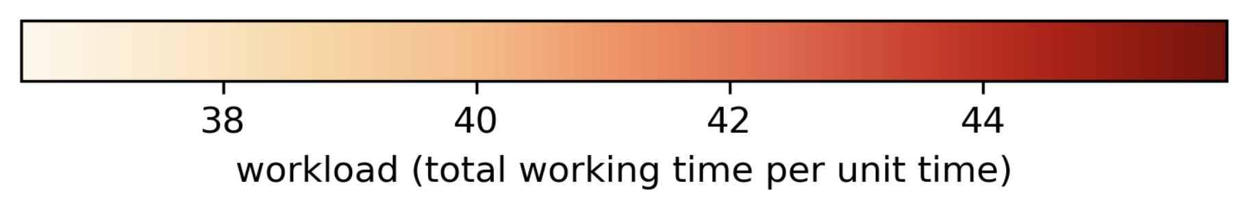
Figure 6: Districting plans for the $6\times 6$ grid districting problem. The workloads are indicated by the depth of the color.

Redistricting $6\times 6$ grid. We first evaluate our algorithm using a synthetic scenario, consisting of a $6\times 6$ grid to be divided into 4 zones, and the decision variable $x\in\{0,1\}^{36\times 4}$. For each region $l$, the arrival rate $\lambda_{l}$ is independently drawn from a standard uniform distribution. Moreover, all regions share an identical service rate of $\mu=1$. We generate an initial data set $\mathcal{D}$ by simulating $n=10,000$ labeled decisions.

Figure 5 demonstrates that our method notably surpasses other baseline methods regarding objective value and convergence speed. Additionally, in Figure 6, we show the optimal districting plans derived from our algorithm alongside those from the baseline methods. It is evident that our approach produces a more balanced plan compared to the other methods.

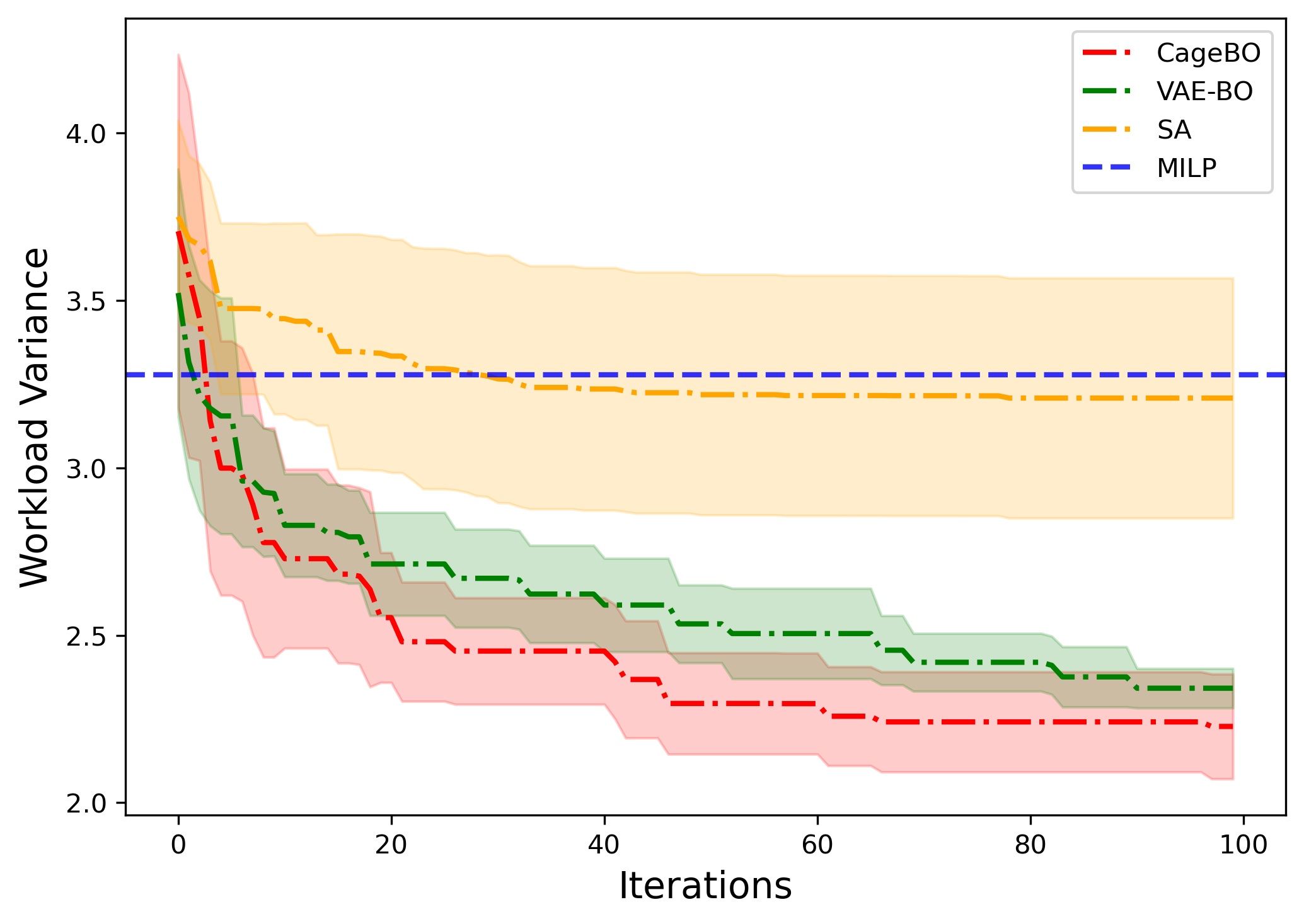
Figure 7: Performance convergence with a 95% confidence interval on the real police districting problem in Atlanta, Georgia.

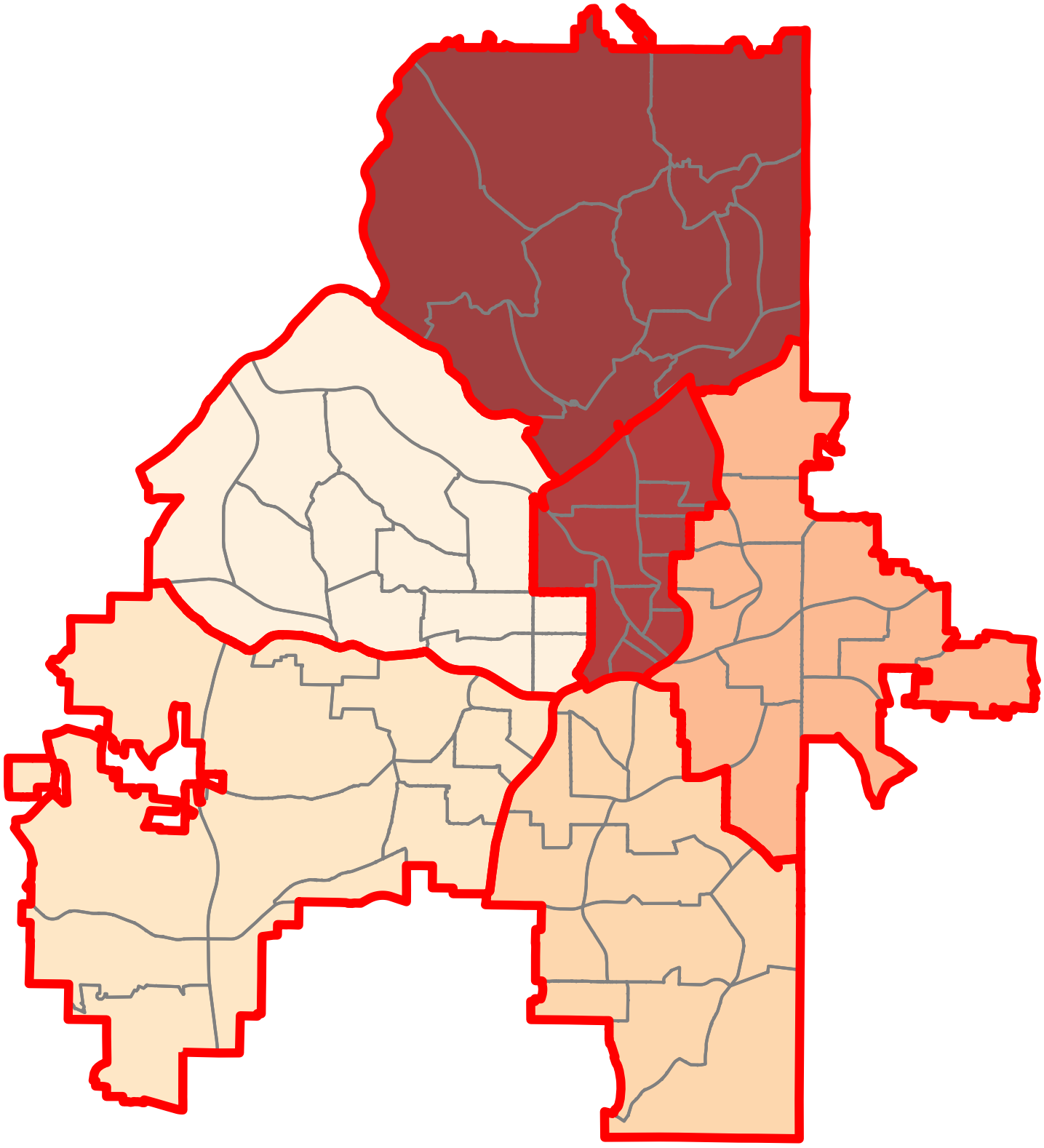
(a) MILP

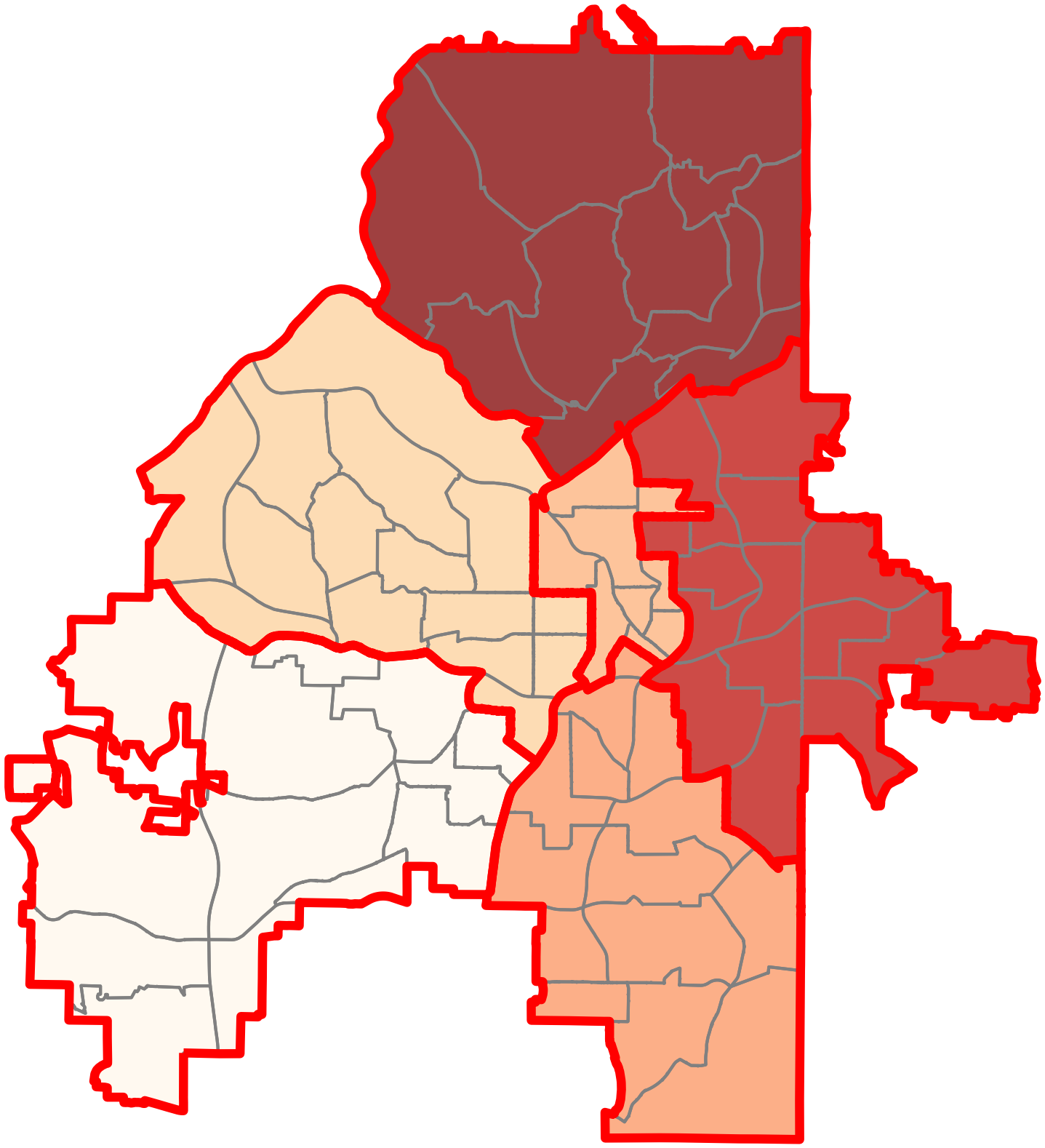
(b) SA

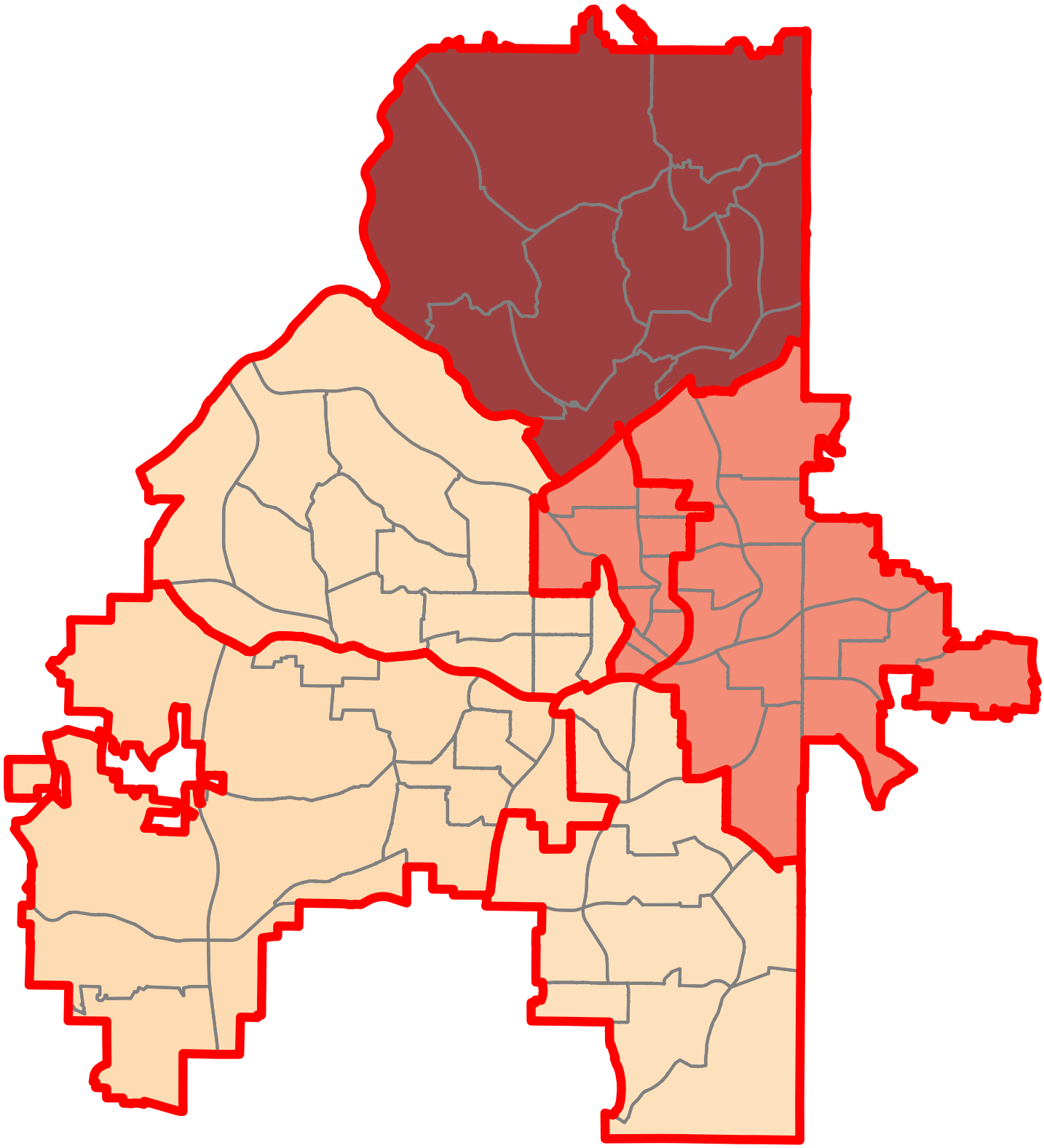
(c) VAE-BO

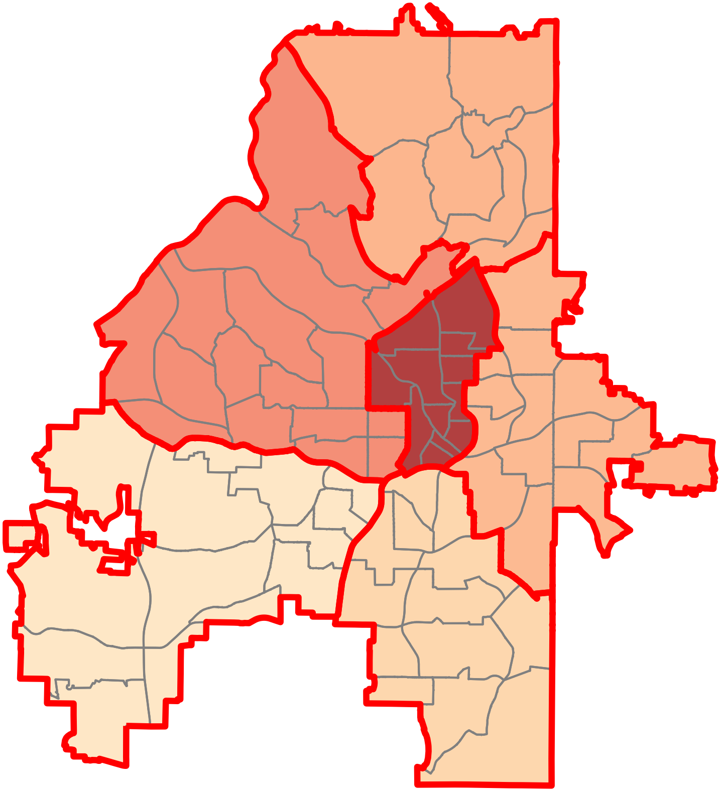
(d) CageBO

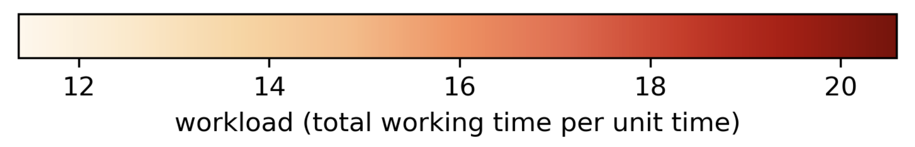
Figure 8: Districting plans for the real police districting problem in Atlanta, Georgia.

Atlanta police redistricting. For the police zone design in Atlanta, there are 78 police service regions that need to be divided into 6 zones, with the decision variable represented as $x\in\{0,1\}^{78\times 6}$. The redistricting of Atlanta’s police zones is constrained by several potential implicit factors. These include contiguity and compactness, as well as other practical constraints that cannot be explicitly defined. One such implicit constraint is the need for changes to the existing plan should be taken in certain local areas. A drastic design change is undesirable because: (1) A large-scale operational change will result in high implementation costs. (2) A radical design change will usually face significant uncertainties and unpredictable risks in future operations. The arrival rate $\lambda_{l}$ and the service rate $\mu$ are estimated using historical 911-calls-for-service data collected in the years 2021 and 2022 (Zhu and Xie,, 2019, 2022; Zhu et al.,, 2022). We generate an initial data set $\mathcal{D}$ by simulating $n=10,000$ labeled decisions which are the neighbors of the existing plan with changes in certain local areas.

Figure 7 displays the convergence of our algorithm in comparison to other baseline methods, showing a consistent reduction in workload variance. Notably, the redistricting plan created by our CageBO algorithm most closely aligns with the actual heuristic policy applied by policymakers, wherein the zone with the highest arrival rate is assigned the largest workload, and the workloads of other zones are well-balanced. As shown in Figure 8, the plan produced by our CageBO algorithm achieves the lowest workload variance, surpassing the VAE-BO and SA algorithms. The superior performance of our CageBO algorithm highlights its capacity to offer critical managerial insights to policymakers, thereby facilitating informed decision-making in real-world applications.

5 Conclusion

In this paper, we introduce and study a new category of optimization problems termed Implicit-Constrained Black-Box Optimization (ICBBO) where constraints are implicit but can be easily verified. This problem is well motivated from real-world police districting problems where districting plans are constrained to socio-economic or political considerations but feasible plans can be easily verified by policymakers. This new ICBBO problem poses more challenges than conventional black-box optimization where existing work cannot be readily applied.

To address this problem, we develop the CageBO algorithm and its core idea is to learn a conditional generative representation of feasible decisions to effectively overcome the complications posed by implicit constraints. In this way, our method can not only learn a good representation of original space but also generate feasible samples that can be used later. Moreover, our algorithm facilitates Bayesian optimization to search in an unconstrained and more compact latent space. Our theoretical analysis shows that CageBO can find global optimal solution by expectation and empirical studies show its effectiveness. Our method can also accommodate traditional constraints by first generating samples that satisfy these constraints and then employing our algorithm for optimization, which yields another potential use case for our framework.

Appendix A Details of theoretical analysis

In this section, we restate our main theorem and show its complete proof afterwards.

Theorem 5 (Restatement of Theorem 1).

After running $T$ iterations, the expected cumulative regret of Algorithm 1 satisfies that

$$\mathbb{E}[R_{T}]=\widetilde{O}(\sqrt{T\gamma_{T}}+\sqrt{d}(n+T)^{\frac{d}{d+1}}),$$ (12)

where $\gamma_{T}$ is the maximum information gain, depending on choice of kernel used in algorithm and $n$ is number of initial observation data points.

Proof.

Our proof starts from the bounding the error term incurred in post-decoder. Let $S$ denote the set of $n$ data points sampled i.i.d. from domain $\mathcal{X}$ and $\epsilon$ denote the expected distance between any data point $x$ and its nearest neighbor $x^{\prime}$ in $\mathcal{X}$, i.e.,

$$\epsilon=\mathbb{E}_{x,\mathcal{X}}[\|x-x^{\prime}\|_{2}].$$ (13)

Recall that $\mathcal{X}\subseteq[0,1]^{d}$ and we discretize it in each dimension using distance $\varepsilon$ and we get $r=(1/\varepsilon)^{d}$ small boxes. Each small box $C_{i}\forall i\in 1,...,r$ is a covering set of the domain. For any two data points in the same box we have $\|x_{1}-x_{2}\|\leq\sqrt{d}\varepsilon$, otherwise, $\|x_{1}-x_{2}\|\leq\sqrt{d}$. Therefore,

$$\epsilon\leq\mathbb{E}_{S}\left[\mathbb{P}\left[\bigcup_{i:C_{i}\cap S=\emptyset}C_{i}\right]\sqrt{d}+\mathbb{P}\left[\bigcup_{i:C_{i}\cap S\neq\emptyset}C_{i}\right]\varepsilon\sqrt{d}\right].$$ (14)

By Lemma 4 and $\mathbb{P}[\cup_{i:C_{i}\cap S\neq\emptyset}C_{i}]\leq 1$ we have

$$\epsilon \leq\sqrt{d}\left(\frac{r}{ne}+\varepsilon\right)$$ (15)

$$=\sqrt{d}\left(\frac{(1/\varepsilon)^{d}}{ne}+\varepsilon\right)$$ (16)

$$\leq 2\sqrt{d}n^{-\frac{1}{d+1}},$$ (17)

where the last step is by choosing $\varepsilon=n^{-1/(d+1)}$.

Next, we try to upper bound the expected cumulative regret. Let $C_{f}$ denote the constant probability that a data point $x_{t}$ is feasible, i.e., $\mathbb{P}[h(x_{t})=1]=C_{f}$, which means with probability $1-C_{f}$, data point $x_{t}$ needs to be post-decoded. By definition of cumulative regret,

$$R_{T} =\sum_{i=1}^{T}f(x_{t})-f(x_{*})=\sum_{i=1}^{T}g(z_{t})-g(z_{*}).$$ (18)

Here are two events: with probability $C_{f}$, $\hat{z}_{t}$ suggested by GP-LCB is feasible and post-decoder is not needed and with probability $1-C_{f}$, $\hat{z}_{t}$ needs to be post-decoded. Thus,

$$\mathbb{E}[R_{T}] =C_{f}\mathbb{E}\left[\sum_{i=1}^{T}g(\hat{z}_{t})-g(z_{*})\right]+(1-C_{f})\mathbb{E}\left[\sum_{i=1}^{T}g(\hat{z}_{t})-g(z_{*})+g(z_{t})-g(\hat{z}_{t})\right],$$ (19)

$$=\mathbb{E}\left[\sum_{i=1}^{T}g(\hat{z}_{t})-g(z_{*})\right]+(1-C_{f})\mathbb{E}\left[\sum_{i=1}^{T}g(z_{t})-g(\hat{z}_{t})\right].$$ (20)

Use Lemma 3 and our assumptions and we have

$$\mathbb{E}[R_{T}] \leq\widetilde{O}(\sqrt{T\gamma_{T}})+O\left(\sum_{t=1}^{T}\epsilon(1-C_{f})C_{p}C_{g}\right)$$ (21)

$$\leq\widetilde{O}(\sqrt{T\gamma_{T}})+O\left(\sum_{t=1}^{T}2\sqrt{d}(1-C_{f})C_{p}C_{g}(n+t)^{-\frac{1}{d+1}}\right)$$ (22)

$$\leq\widetilde{O}(\sqrt{T\gamma_{T}}+\sqrt{d}(n+T)^{\frac{d}{d+1}}),$$ (23)

where the second inequality is due to eq. (17) and number of data points is $n+t$ since the algorithm keeps adding points to $\mathcal{Z}$. ∎

Appendix B Implementation details of the conditional generative model

Here we present the derivation of the the evidence lower bound of the log-likelihood in Eq (3).

Given observation $x$, feasibility $c$, and the latent random variable $z$, let $p(x|c)$ denote the likelihood of $x$ conditioned on feasibility $c$, and $p(x|z,c)$ denote the conditional distribution of $x$ given latent variable $z$ and its feasibility $c$. Let $p(z|c)$ denote the conditional prior of the latent random variable $z$ given its feasibility $c$, and $q(z|x,c)$ denote the posterior distribution of $z$ after observing $x$ and its feasibility $c$. The likelihood of observation $x$ given $c$ can be written as:

$$p(x|c) =\int p(x,z|c)dz=\underset{q(z|x,c)}{\mathbb{E}}\left[\frac{p(x,z|c)}{q(z|x,c)}\right].$$ (24)

By taking the logarithm on both sides and then applying Jensen’s inequality, we can get the lower bound of the log-likelihood $\mathcal{L}_{\mathrm{ELBO}}$ as follows:

$$\log p(x|c) =\log\underset{q(z|x,c)}{\mathbb{E}}\left[\frac{p(x,z|c)}{q(z|x,c)}\right]$$ (25)

$$\geq\underset{q(z|x,c)}{\mathbb{E}}\left[\log\frac{p(x,z|c)}{q(z|x,c)}\right]$$ (26)

$$=\underset{q(z|x,c)}{\mathbb{E}}\left[\log\frac{p(x|z,c)p(z|c)}{q(z|x,c)}\right]$$ (27)

$$=\underset{q(z|x,c)}{\mathbb{E}}\left[\log{p(x|z,c)}\right]+\underset{q(z|x,c)}{\mathbb{E}}\left[\log\frac{p(z|c)}{q(z|x,c)}\right]$$ (28)

$$=\underset{q(z|x,c)}{\mathbb{E}}\left[\log p(x|z,c)\right]-\mathrm{D}_{\mathrm{KL}}\left(q(z|x,c)\|p(z|c)\right).$$ (29)

In practice, we add a weight function $w(c)$ on the first term based on feasibility $c$ and a hyperparameter $\eta$ on the second term to modulate the penalization ratio.

$$\mathcal{L}_{\mathrm{ELBO}}=w(c)\underset{q(z|x,c)}{\mathbb{E}}\left[\log p(x|z,c)\right]-\eta\mathrm{D}_{\mathrm{KL}}\left(q(z|x,c)\|p(z|c)\right).$$ (30)

In practice, we approximate the conditional distribution $q(z|x,c)$ and $p(x|z,c)$ by building the ${\mathrm{encoder}}_{\phi}$ and ${\mathrm{decoder}}_{\theta}$ neural networks, and denote the approximated conditional distribution to be $q_{\phi}(z|x,c)$ and $p_{\theta}(x|z,c)$ respectively. In our formulation, the prior of the latent variable is influenced by the feasibility $c$; however, this constraint can be easily relaxed to make the latent variables statistically independent of their labels, adopting a standard Gaussian distribution $\mathcal{N}(0,I)$. Both $q(z|x,c)$ and $p(x|z,c)$ are typically modeled as Gaussian distributions to facilitate closed-form KL divergence computation. Specifically, we introduce generator layers $l(\epsilon,x,c)$ and $l(\epsilon)$ to represent $q(z|x,c)$ and $p(z)$, respectively, transforming the random variable $\epsilon\sim\mathcal{N}(0,I)$ using the reparametrization trick (Sohl-Dickstein et al.,, 2015). The log-likelihood of the first term is realized as the reconstruction loss, computed with the training data.

Appendix C Details of baseline settings

1. SA: Please refer to Algorithm 2.

2. VAE-BO: Please refer to Algorithm 1 in (Eissman et al.,, 2018).

3. MILP: Please refer to Section E.3 in the Appendix of (Zhu et al.,, 2022).

  Input: Objective function $\hat{f}$; Initial solution $x$; Hyper-parameters $\alpha=0.8$, $C_{init}=1$, $T$. $x^{*}\leftarrow x$, $t\leftarrow 0$, $C\leftarrow C_{init}$;

  while $t<T$ do

     $x^{\prime}\leftarrow\textbf{Neighbour}(x)$; // Randomly pick a neighbour

     $\Delta\leftarrow\hat{f}(x^{\prime})-\hat{f}(x)$;

     $r\sim\text{Uniform}(0,1)$;

     if $\Delta<0$ or $r<\exp(-\Delta/C)$ then

        $x\leftarrow x^{\prime}$;

     end if

     if $\hat{f}(x^{\prime})<\hat{f}(x^{*})$ then

        $x^{*}\leftarrow x^{\prime}$;

     end if

     $C\leftarrow\alpha C$, $t\leftarrow t+1$; // Cooling temperature

  end whilereturn $x^{*}$

Algorithm 2 Simulated Annealing (SA)

References

- Antonova et al., (2020) Antonova, R., Rai, A., Li, T., and Kragic, D. (2020). Bayesian optimization in variational latent spaces with dynamic compression. In Kaelbling, L. P., Kragic, D., and Sugiura, K., editors, Proceedings of the Conference on Robot Learning, volume 100 of Proceedings of Machine Learning Research, pages 456–465. PMLR.
- Ariafar et al., (2019) Ariafar, S., Coll-Font, J., Brooks, D., and Dy, J. (2019). Admmbo: Bayesian optimization with unknown constraints using admm. Journal of Machine Learning Research, 20(123):1–26.
- Audet et al., (2020) Audet, C., Caporossi, G., and Jacquet, S. (2020). Binary, unrelaxable and hidden constraints in blackbox optimization. Operations Research Letters, 48(4):467–471.
- Binois and Wycoff, (2022) Binois, M. and Wycoff, N. (2022). A survey on high-dimensional gaussian process modeling with application to bayesian optimization. ACM Transactions on Evolutionary Learning and Optimization, 2(2):1–26.
- Chandak et al., (2020) Chandak, A., Dey, D., Mukhoty, B., and Kar, P. (2020). Epidemiologically and socio-economically optimal policies via bayesian optimization. Transactions of the Indian National Academy of Engineering, 5:117–127.
- Char et al., (2019) Char, I., Chung, Y., Neiswanger, W., Kandasamy, K., Nelson, A. O., Boyer, M., Kolemen, E., and Schneider, J. (2019). Offline contextual bayesian optimization. Advances in Neural Information Processing Systems, 32.
- Chen et al., (2023) Chen, C., Beckham, C., Liu, Z., Liu, X., and Pal, C. (2023). Parallel-mentoring for offline model-based optimization. arXiv preprint arXiv:2309.11592.
- Choi et al., (2000) Choi, T. D., Eslinger, O. J., Kelley, C. T., David, J. W., and Etheridge, M. (2000). Optimization of automotive valve train components with implicit filtering. Optimization and Engineering, 1:9–27.
- Dai et al., (2022) Dai, Z., Shu, Y., Low, B. K. H., and Jaillet, P. (2022). Sample-then-optimize batch neural thompson sampling. Advances in Neural Information Processing Systems, 35:23331–23344.
- Deshwal and Doppa, (2021) Deshwal, A. and Doppa, J. (2021). Combining latent space and structured kernels for bayesian optimization over combinatorial spaces. Advances in Neural Information Processing Systems, 34:8185–8200.
- Eissman et al., (2018) Eissman, S., Levy, D., Shu, R., Bartzsch, S., and Ermon, S. (2018). Bayesian optimization and attribute adjustment. In Proc. 34th Conference on Uncertainty in Artificial Intelligence.
- Eriksson and Poloczek, (2021) Eriksson, D. and Poloczek, M. (2021). Scalable constrained bayesian optimization. In Banerjee, A. and Fukumizu, K., editors, Proceedings of The 24th International Conference on Artificial Intelligence and Statistics, volume 130 of Proceedings of Machine Learning Research, pages 730–738. PMLR.
- Gardner et al., (2014) Gardner, J. R., Kusner, M. J., Xu, Z. E., Weinberger, K. Q., and Cunningham, J. P. (2014). Bayesian optimization with inequality constraints. In ICML, volume 2014, pages 937–945.
- Gelbart et al., (2014) Gelbart, M. A., Snoek, J., and Adams, R. P. (2014). Bayesian optimization with unknown constraints. In 30th Conference on Uncertainty in Artificial Intelligence, UAI 2014, pages 250–259.
- Guo et al., (2023) Guo, J., Ranković, B., and Schwaller, P. (2023). Bayesian optimization for chemical reactions. Chimia, 77(1/2):31–31.
- Jordan et al., (1999) Jordan, M. I., Ghahramani, Z., Jaakkola, T. S., and Saul, L. K. (1999). An introduction to variational methods for graphical models. Machine learning, 37:183–233.
- Kandasamy et al., (2020) Kandasamy, K., Vysyaraju, K. R., Neiswanger, W., Paria, B., Collins, C. R., Schneider, J., Poczos, B., and Xing, E. P. (2020). Tuning hyperparameters without grad students: Scalable and robust bayesian optimisation with dragonfly. The Journal of Machine Learning Research, 21(1):3098–3124.
- Keane, (1994) Keane, A. (1994). Experiences with optimizers in structural design. In In Proceedings of the conference on adaptive computing in engineering design and control, volume 94, pages 14–27.
- Kingma and Ba, (2015) Kingma, D. and Ba, J. (2015). Adam: A method for stochastic optimization. In International Conference on Learning Representations (ICLR), San Diega, CA, USA.
- Kirkpatrick et al., (1983) Kirkpatrick, S., Gelatt Jr, C. D., and Vecchi, M. P. (1983). Optimization by simulated annealing. science, 220(4598):671–680.
- Krishnamoorthy et al., (2023) Krishnamoorthy, S., Mashkaria, S. M., and Grover, A. (2023). Diffusion models for black-box optimization. arXiv preprint arXiv:2306.07180.
- Laguna and Martí, (2005) Laguna, M. and Martí, R. (2005). Experimental testing of advanced scatter search designs for global optimization of multimodal functions. Journal of Global Optimization, 33:235–255.
- Larson, (1974) Larson, R. C. (1974). A hypercube queuing model for facility location and redistricting in urban emergency services. Computers & Operations Research, 1(1):67–95.
- Larson and Odoni, (1981) Larson, R. C. and Odoni, A. R. (1981). Urban operations research.
- Letham et al., (2019) Letham, B., Karrer, B., Ottoni, G., and Bakshy, E. (2019). Constrained Bayesian Optimization with Noisy Experiments. Bayesian Analysis, 14(2):495 – 519.
- Liu and Wang, (2023) Liu, C. and Wang, Y.-X. (2023). Global optimization with parametric function approximation. In International Conference on Machine Learning, pages 22113–22136. PMLR.
- Luong et al., (2019) Luong, P., Gupta, S., Nguyen, D., Rana, S., and Venkatesh, S. (2019). Bayesian optimization with discrete variables. In AI 2019: Advances in Artificial Intelligence: 32nd Australasian Joint Conference, Adelaide, SA, Australia, December 2–5, 2019, Proceedings 32, pages 473–484. Springer.
- Maus et al., (2022) Maus, N., Jones, H., Moore, J., Kusner, M. J., Bradshaw, J., and Gardner, J. (2022). Local latent space bayesian optimization over structured inputs. Advances in Neural Information Processing Systems, 35:34505–34518.
- Pardalos et al., (2021) Pardalos, P. M., Rasskazova, V., Vrahatis, M. N., et al. (2021). Black Box Optimization, Machine Learning, and No-Free Lunch Theorems. Springer.
- Pinheiro Cinelli et al., (2021) Pinheiro Cinelli, L., Araújo Marins, M., Barros da Silva, E. A., and Lima Netto, S. (2021). Variational autoencoder. In Variational Methods for Machine Learning with Applications to Deep Networks, pages 111–149. Springer.
- Seeger, (2004) Seeger, M. (2004). Gaussian processes for machine learning. International journal of neural systems, 14(02):69–106.
- Shalev-Shwartz and Ben-David, (2014) Shalev-Shwartz, S. and Ben-David, S. (2014). Understanding machine learning: From theory to algorithms. Cambridge university press.
- Shirabe, (2009) Shirabe, T. (2009). Districting modeling with exact contiguity constraints. Environment and Planning B: Planning and Design, 36(6):1053–1066.
- Sohl-Dickstein et al., (2015) Sohl-Dickstein, J., Weiss, E., Maheswaranathan, N., and Ganguli, S. (2015). Deep unsupervised learning using nonequilibrium thermodynamics. In International conference on machine learning, pages 2256–2265. PMLR.
- Sohn et al., (2015) Sohn, K., Lee, H., and Yan, X. (2015). Learning structured output representation using deep conditional generative models. Advances in neural information processing systems, 28.
- Srinivas et al., (2010) Srinivas, N., Krause, A., Kakade, S., and Seeger, M. (2010). Gaussian process optimization in the bandit setting: No regret and experimental design. In Proceedings of the 27th International Conference on Machine Learning, pages 1015–1022.
- Srinivas et al., (2009) Srinivas, N., Krause, A., Kakade, S. M., and Seeger, M. (2009). Gaussian process optimization in the bandit setting: No regret and experimental design. arXiv preprint arXiv:0912.3995.
- Turner et al., (2021) Turner, R., Eriksson, D., McCourt, M., Kiili, J., Laaksonen, E., Xu, Z., and Guyon, I. (2021). Bayesian optimization is superior to random search for machine learning hyperparameter tuning: Analysis of the black-box optimization challenge 2020. In NeurIPS 2020 Competition and Demonstration Track, pages 3–26. PMLR.
- Ueno et al., (2016) Ueno, T., Rhone, T. D., Hou, Z., Mizoguchi, T., and Tsuda, K. (2016). Combo: An efficient bayesian optimization library for materials science. Materials discovery, 4:18–21.
- van Veenstra and Kotterink, (2017) van Veenstra, A. F. and Kotterink, B. (2017). Data-driven policy making: The policy lab approach. In Electronic Participation: 9th IFIP WG 8.5 International Conference, ePart 2017, St. Petersburg, Russia, September 4-7, 2017, Proceedings 9, pages 100–111. Springer.
- Varol et al., (2012) Varol, A., Salzmann, M., Fua, P., and Urtasun, R. (2012). A constrained latent variable model. In 2012 IEEE conference on computer vision and pattern recognition, pages 2248–2255. Ieee.
- Wan et al., (2021) Wan, X., Nguyen, V., Ha, H., Ru, B., Lu, C., and Osborne, M. A. (2021). Think global and act local: Bayesian optimisation over high-dimensional categorical and mixed search spaces. arXiv preprint arXiv:2102.07188.
- Williams and Rasmussen, (2006) Williams, C. K. and Rasmussen, C. E. (2006). Gaussian processes for machine learning. MIT press Cambridge, MA.
- Xie et al., (2021) Xie, W., Nie, W., Saffari, P., Robledo, L. F., Descote, P.-Y., and Jian, W. (2021). Landslide hazard assessment based on bayesian optimization–support vector machine in nanping city, china. Natural Hazards, 109(1):931–948.
- Xing and Hua, (2022) Xing, W. and Hua, C. (2022). Optimal unit locations in emergency service systems with bayesian optimization. In INFORMS International Conference on Service Science, pages 439–452. Springer.
- Yu et al., (2021) Yu, S., Qing, Q., Zhang, C., Shehzad, A., Oatley, G., and Xia, F. (2021). Data-driven decision-making in covid-19 response: A survey. IEEE Transactions on Computational Social Systems, 8(4):1016–1029.
- Zhang et al., (2020) Zhang, Y., Apley, D. W., and Chen, W. (2020). Bayesian optimization for materials design with mixed quantitative and qualitative variables. Scientific reports, 10(1):4924.
- Zhu et al., (2020) Zhu, S., Bukharin, A. W., Lu, L., Wang, H., and Xie, Y. (2020). Data-driven optimization for police beat design in south fulton, georgia. arXiv preprint arXiv:2004.09660.
- Zhu et al., (2022) Zhu, S., Wang, H., and Xie, Y. (2022). Data-driven optimization for atlanta police-zone design. INFORMS Journal on Applied Analytics, 52(5):412–432.
- Zhu and Xie, (2019) Zhu, S. and Xie, Y. (2019). Crime event embedding with unsupervised feature selection. In ICASSP 2019-2019 IEEE International Conference on Acoustics, Speech and Signal Processing (ICASSP), pages 3922–3926. IEEE.
- Zhu and Xie, (2022) Zhu, S. and Xie, Y. (2022). Spatiotemporal-textual point processes for crime linkage detection. The Annals of Applied Statistics, 16(2):1151–1170.