Overview of AdaBoost: Reconciling its views to better understand its dynamics

Abstract

Boosting methods have been introduced in the late 1980’s. They were born following the theoritical aspect of PAC learning. The main idea of boosting methods is to combine weak learners to obtain a strong learner. The weak learners are obtained iteratively by an heuristic which tries to correct the mistakes of the previous weak learner. In 1995, Freund and Schapire [18] introduced AdaBoost, a boosting algorithm that is still widely used today. Since then, many views of the algorithm have been proposed to properly tame its dynamics. In this paper, we will try to cover all the views that one can have on AdaBoost. We will start with the original view of Freund and Schapire before covering the different views and unify them with the same formalism. We hope this paper will help the non-expert reader to better understand the dynamics of AdaBoost and how the different views are equivalent and related to each other.
Keywords: Boosting, AdaBoost, dynamical systems, PAC learning, gradient descent, mirror descent, additive models, entropy projection, diversity, margin, generalization error, kernel methods, product of experts, interpolating classifiers, double descent

1 Introduction, problematic & notations

1.1 Introduction

Machine learning is a dynamic field that encompasses a wide range of algorithms and methodologies, aiming to enable computational systems to learn from data and make predictions or decisions without being explicitly programmed. The growth of computational power, the availability of vast amounts of data, and advancements in statistical and algorithmic techniques have propelled the field of machine learning to new heights [29, 25]. The application of machine learning methods are ubiquitous in our daily lives, from the personalized recommendations on internet platforms [51, 46, 45] to medicine [6, 49, 8], finance [12, 14, 9, 23], or autonomous driving [27, 48, 33]. One prominent subset of machine learning methods that has gained considerable attention and achieved remarkable success in various applications is boosting [18, 44].

At its core, machine learning involves the development of models that can automatically extract patterns and insights from data. These models learn from experience, iteratively refining their performance through exposure to labeled examples. By analyzing patterns and relationships within the data, machine learning algorithms can make accurate predictions on new, unseen instances, thereby uncovering hidden knowledge and informing decision-making processes.

Boosting algorithms are a class of machine learning methods (more precisely of ensemble methods [11, 53, 41]) that aim to enhance the performance of weak learners by iteratively combining their predictions to create a more powerful and accurate model [18, 44]. These methods were introduced in the 1990’s and have since emerged as a cornerstone of contemporary machine learning research. Boosting algorithms iteratively train a sequence of weak models, each focusing on the instances that were previously misclassified or had the largest prediction errors. By assigning higher weights to these challenging instances, subsequent models within the boosting framework can effectively address their misclassification and improve overall accuracy.

One of the key advantages of boosting methods is their ability to adaptively allocate resources to challenging examples, thereby mitigating the impact of noise and outliers. By emphasizing the instances that are difficult to classify, boosting algorithms excel at capturing complex decision boundaries and achieving high predictive performance. Furthermore, boosting methods are versatile and can be applied to a variety of learning tasks, including classification, regression, and ranking problems.

Boosting algorithms come in various flavors, each with its unique characteristics and strengths. One of the earliest and most influential boosting methods is AdaBoost [18], short for Adaptive Boosting. AdaBoost iteratively adjusts the weights of misclassified instances, with subsequent models paying greater attention to these misclassified examples. Another popular boosting method is Gradient Boosting [35, 4, 21], which leverages the concept of gradient descent to optimize a loss function by adding weak models in a stage-wise manner. XGBoost [7, 36, 10] and LightGBM [26, 47, 50] are notable implementations of gradient boosting algorithms that have gained widespread adoption due to their scalability and high performance.

1.2 Problematic

Boosting methods have emerged for the first ones in the early 1990’s, and the proper modern formalization of boosting methods has been made in 1990 by Schapire [43]. At that time, boosting methods were seen as PAC learning algorithms. Later, Freund and Schapire [17] collaborated to work deeper on boosting algorithms, and in 1995, they introduced AdaBoost [18], which is still widely used today. Since then, many researchers have tried to understand the dynamics of AdaBoost which were not sufficiently understood. To this day, there is still a lot that we do not know about AdaBoost, especially about the convergence properties of the algorithm when we increase the number of weak learners [3]. The goal of this paper was in the first place to try to answer the question of the cyclic behavior of AdaBoost which was proven in some cases in 2004 by Rudin et al. [40], and that can be observed in many toy examples (see Fig. 2). However, the same authors addressed an open problem in 2012 [39] for the general case: Does AdaBoost always cycle? Some answers have been found very recently, in 2023, by Belanich and Ortiz [3]. Indeed, by studying the ergodic dynamics of AdaBoost, the authors have shown this conjecture as an intermediate result, which we will quickly present in the last subsection.

Yet, this overview aims to cover all views that one can have on AdaBoost. We tried to use the same formalism for all views, to try and unify them.

1.3 Notations

In all what follows, we will consider a classification problem. We will denote by $\mathcal{X}$ the input space, and by $\mathcal{Y}$ the output space. $\mathcal{X}$ is a compact subset of $\mathbb{R}^{d}$, and $\mathcal{Y}$ is a finite set, which will be $\{-1,1\}$ if the problem is binary, and $\{1,\dots,K\}$ if the problem is multiclass. The sequence of weights produced by AdaBoost will be denoted $W_{0},\dots,W_{T-1}$, and the sequence of classifiers will be denoted $h_{1},\dots,h_{T}$, where $T$ is the number of iterations of the algorithm. The final classifier will be denoted $H$. We will denote by $\mathbbm{1}_{A}$ the indicator function of the set $A$. For binary problems, we will use the notation $\eta$ or $\eta_{h}$ to denote the vector $(y_{1}h(x_{1}),\dots,y_{m}h(x_{m}))$ which we call a dichotomy. $\eta_{h}(i)$ is 1 if the classifier $h$ is right, and $-1$ if it is wrong. Also, we will denote by $\lambda$ the standard Lebesgue measure.

2 Views of AdaBoost

2.1 The original view: a PAC learning algorithm

2.1.1 What is a PAC learning algorithm?

Definition 2.1.1 (PAC learning algorithm).

In our setting, we say that a hypothesis space $\mathcal{H}$ is PAC learnable if there exists an algorithm $A$ such that: • For any distribution $D$ over $\mathcal{X}$, and for any $0<\epsilon,\delta<\frac{1}{2}$, the algorithm $A$ outputs a classifier $h\in\mathcal{H}$ such that with probability at least $1-\delta$, we have: $$\mathbb{P}_{(x,y)\sim D}(h(x)\neq y)\leq\epsilon$$ (1) • The number of examples $m$ needed to achieve this bound is polynomial in $\frac{1}{\epsilon}$, $\frac{1}{\delta}$ and $d$.

2.1.2 AdaBoost: the original formulation

The first view, when AdaBoost was introduced, was to see it as a PAC learning algorithm. The idea was to create a boosting algorithm that iteratively takes into accound the errors made by the previous classifiers, and to try to correct them. Freund and Schapire [18] proposed the following algorithm, which is the original formulation of AdaBoost. They also verified that the algorithm is a PAC learning algorithm, and give bounds on the number of examples needed to achieve a given accuracy. The pseudo-code implementation of the algorithm is given in Alg. 1.

Data: $(x_{1},y_{1}),\dots,(x_{m},y_{m})\in\mathcal{X}\times\{-1,1\}$ Initialize $W_{0}(i)=\frac{1}{m}$ for $i=1,\dots,m$ for $t=1,\dots,T$ do        Train a weak learner $h_{t}:\mathcal{X}\rightarrow\{-1,1\}$ w.r.t. the distribution $W_{t-1}$        Compute $\displaystyle\epsilon_{t}=\sum_{i=1}^{m}W_{t-1}(i)\mathbbm{1}_{h_{t}(x_{i})\neq y_{i}}$ the weighted error of $h_{t}$        Compute $\displaystyle\alpha_{t}=\frac{1}{2}\log\frac{1-\epsilon_{t}}{\epsilon_{t}}$        Update $\displaystyle W_{t}(i)=\frac{W_{t-1}(i)\exp(-\alpha_{t}y_{i}h_{t}(x_{i}))}{Z_{t}}$ for $i=1,\dots,m$, where $\displaystyle Z_{t}=\sum_{i=1}^{m}W_{t-1}(i)\exp(-\alpha_{t}y_{i}h_{t}(x_{i}))$ end for return $\displaystyle H:x\in\mathcal{X}\mapsto\mathrm{sign}\left(\sum_{t=1}^{T}\alpha_{t}h_{t}(x)\right)\in\mathcal{Y}$ Algorithm 1 Original formulation of AdaBoost (discrete) for a binary classification problem

Remark 1.

Freund and Schapire designed this algorithm for weak learners, i.e. classifiers that have an error rate slightly better than random guessing. They proved that if the weak learners error rates are $\epsilon_{1},\dots,\epsilon_{T}$, then the error rate of the final classifier is bounded by $$\epsilon\leq 2^{T}\prod_{t=1}^{T}\sqrt{\epsilon_{t}(1-\epsilon_{t})}$$ (2)

Remark 2.

The first nad most natural set of classifiers that come to mind when we think about weak learners are decision stumps, i.e. classifiers that are constant on a half-space, and constant on the other half-space. Most of AdaBoost applications in practice use decision stumps as weak learners. We also can think of decision trees of an arbitrary depth as weak learners, but in practice, they may not be used because they are slower to train.

Remark 3.

The first few things we can observe are that first the final classifier does not take in consideration the potential relevance (to be defined) of each classifier in the final vote (the weights of the classifiers are all equal to $1$), and second that the sequence of weights are updated only considering the error made by the previous classifier, and not the ones before. We can easily see that both sequence of weights and classifiers are order 1 Markov chains, therefore we can legitimately ask ourselves if the algorithm can get stuck in cycles, which can be the case in some examples [38].

However, at that time, Freund and Schapire did not give any insight of how they chose their updating rule for the weights. They just said that they wanted to correct the errors made by the previous classifier, and that they wanted to give more importance to the examples that were misclassified. In short, they designed a heuristic algorithm, and proved that it was a PAC learning algorithm. Later on, it appeared that AdaBoost does not only come from a heuristic, but also from a theoritical point of view, as we will see in the next sections.

Freund and Schapire also gave a multiclass version of AdaBoost in 1996 [19], which base on the same heuristic. We give the algorithm in Alg. 2.

Data: $(x_{1},y_{1}),\dots,(x_{m},y_{m})\in\mathcal{X}\times\{1,\dots,K\}$ Initialize $W_{0}(i)=\frac{1}{m}$ for $i=1,\dots,m$ for $t=1,\dots,m$ do        Train a weak learner $h_{t}:\mathcal{X}\rightarrow\{1,\dots,K\}$ w.r.t. the distribution $W_{t-1}$        Compute $\epsilon_{t}=\sum_{i=1}^{m}W_{t-1}(i)\mathbbm{1}_{h_{t}(x_{i})\neq y_{i}}$ the weighted error of $h_{t}$        Compute $\alpha_{t}=\frac{1-\epsilon_{t}}{\epsilon_{t}}$        Update $W_{t}(i)=\frac{W_{t-1}(i)(\alpha_{t}\mathbbm{1}_{h_{t}(x_{i})=y_{i}}+\mathbbm{1}_{h_{t}(x_{i})\neq y_{i}})}{Z_{t}}$ for $i=1,\dots,m$, where $Z_{t}=\sum_{i=1}^{m}W_{t-1}(i)\exp(-\alpha_{t}\mathbbm{1}_{h_{t}(x_{i})=y_{i}})$ end for return $H:x\in\mathcal{X}\mapsto\operatorname*{arg\,max}_{y\in\mathcal{Y}}\sum_{t=1}^{T}\left(\log\frac{1}{\alpha_{t}}\right)\mathbbm{1}_{h_{t}(x)=y}$ Algorithm 2 Original formulation of AdaBoost (discrete) for a multiclass classification problem

2.1.3 Real AdaBoost

The original formulation of AdaBoost is a discrete version of the algorithm. However, it is possible to define a real version of AdaBoost, as Freund and Schapire did [19]. The main difference is that the weak learners are not restricted to output only $\{-1,1\}$, but are functionals $h:X\times Y\rightarrow[0,1]$.

Definition 2.1.2 (Pseudo-loss and Update Rule for real AdaBoost).

To each couple $(x,y)$, we associate a plausibility $h(x,y)$ that $x$ belongs to the class $y$ (plausibility instead of probability, because it is not one). We then define the pseudo-loss $\epsilon_{t}$ of $h_{t}$ at iteration $t$ as: $$\epsilon_{t}=\frac{1}{2}\sum_{(i,y):y\neq y_{i}}W_{t-1}(i,y)(1-h_{t}(x_{i},y_{i})+h_{t}(x_{i},y))$$ (3) where $W_{t-1}(i,y)$ is the weight of the couple $(x_{i},y)$ at iteration $t-1$. Finally, we can define the weight update rule, following the same principle, as: $\displaystyle W_{0}(i,y)$ $\displaystyle=\frac{1}{mK},\quad\forall i\in\{1,\dots,m\},\forall y\in\mathcal{Y}$ (4) $\displaystyle W_{t}(i,y)$ $\displaystyle=\frac{W_{t-1}(i,y)\alpha_{t}^{\frac{1}{2}(1-h_{t}(x_{i},y_{i})+h_{t}(x_{i},y))}}{Z_{t}}$ where $Z_{t}$ is a normalization factor.

The algorithm now writes as in Alg. 3.

Data: $(x_{1},y_{1}),\dots,(x_{m},y_{m})\in\mathcal{X}\times\mathcal{Y}$ Initialize $W_{0}(i,y)=\frac{1}{mK}$ for $i=1,\dots,m$, $y\in\mathcal{Y}$ for $t=1,\dots,T$ do        Train a weak learner $h_{t}:\mathcal{X}\times\mathcal{Y}\rightarrow[0,1]$ w.r.t. the distribution $W_{t-1}$        Compute $\epsilon_{t}=\frac{1}{2}\sum_{(i,y):y\neq y_{i}}W_{t-1}(i,y)(1-h_{t}(x_{i},y_{i})+h_{t}(x_{i},y))$        Compute $\alpha_{t}=\frac{1-\epsilon_{t}}{\epsilon_{t}}$        Update $W_{t}(i,y)=\frac{W_{t-1}(i,y)\alpha_{t}^{\frac{1}{2}(1-h_{t}(x_{i},y_{i})+h_{t}(x_{i},y))}}{Z_{t}}$        end for return $H:x\in\mathcal{X}\mapsto\operatorname*{arg\,max}_{y\in\mathcal{Y}}\sum_{t=1}^{T}\left(\log\frac{1}{\alpha_{t}}\right)h_{t}(x,y)$ Algorithm 3 Original formulation of AdaBoost (real) for a multiclass classification problem

2.2 AdaBoost as successive optimization problems

2.2.1 AdaBoost as a gradient descent

In 1999, Mason et al. [32] proposed a new view of boosting. They saw any boosting algorithm, including AdaBoost, as a gradient descent on the set of linear combinations of classifiers in $\mathcal{H}$.

Definition 2.2.1 (Optimization problem for AdaBoost as a gradient descent).

Let $\langle,\rangle$ be an inner product on $\mathrm{Span}(\mathcal{H})$. Define a cost function $C:\mathrm{Span}(\mathcal{H})\rightarrow\mathbb{R}$. We define the optimization problem associated to the cost function $C$ as: $$\min_{H\in\mathrm{Span}(\mathcal{H})}C(H)$$ (5)

Definition 2.2.2 (Margin and margin cost-functionals).

We define the margin of a classifier $h\in\mathcal{H}$ as $$\gamma(h)=\langle h(x),y\rangle=\frac{1}{m}\sum_{i=1}^{m}h(x_{i})y_{i}.$$ (6) and the margin cost-functionals as $$C(h)=\frac{1}{m}\sum_{i=1}^{m}c(h(x_{i})y_{i})$$ (7) where $c$ is a differentiable function of the margin $\gamma$.

We can now prove Thm. 2.2.3.

Theorem 2.2.3 (AdaBoost as a gradient descent).

AdaBoost is a gradient descent algorithm on the optimization problem defined in Def. 2.2.1 for the margin-cost functional $C$ with $c(\gamma)=\exp{-\gamma}$.

[Proof.]At each iteration $t$, we will denote by $H_{t}$ the current resulting classifier, which writes

$$H_{t}=\sum_{i=1}^{t}\alpha_{i}h_{i}$$ (8)

Now, consider the inner product (recall that $m$ is the number of training examples)

$$\langle h,g\rangle=\frac{1}{m}\sum_{i=1}^{m}h(x_{i})g(x_{i}).$$ (9)

For AdaBoost, fix $c(\gamma)=\exp(-\gamma)$, thus the cost function we want to optimize over the set of classifiers $\mathcal{H}$ is

$$C(h)=\frac{1}{m}\sum_{i=1}^{m}\exp(-y_{i}h(x_{i}))$$ (10)

To find the next classifier in the sequence, we have to find the classifier $h_{t}$ that minimizes the weighted error $\epsilon_{t}$. With a reasonable cost function $c$ of the margin (i.e. monotonic decreasing), it is equivalent to finding the classifier $h_{t}$ that maximizes $-\langle\nabla C(h_{t-1}),h_{t}\rangle$. Indeed, we have on the one hand

$$\nabla C(h)=-\frac{1}{m}y_{i}e^{-y_{i}h(x_{i})}\mathbbm{1}_{x=x_{i}}$$ (11)

which leads to

$$-\langle\nabla C(H_{t-1}),h_{t}\rangle =\frac{1}{m^{2}}\sum_{i=1}^{m}y_{i}h_{t}(x_{i})e^{-y_{i}H_{t-1}(x_{i})}$$ (12)

$$\propto\frac{1}{m^{2}}\sum_{i=1}^{m}y_{i}h_{t}(x_{i})W_{t-1}(x_{i})$$

up to a normalization constant. That means that maximizing $-\langle\nabla C(H_{t-1}),h_{t}\rangle$ (i.e. gradient descent step) is equivalent to minimizing $\sum_{i=1}^{m}W_{t-1}(x_{i})\mathbbm{1}_{h_{t}(x_{i})\neq y_{i}}$, which is the weighted error of $h_{t}$. Thus, the update rule for this gradient descent is the same as the one of AdaBoost. ∎ That new view of AdaBoost is interesting because it gives both theoritical and intuitive justification of the algorithm. For some cost function $c$ that ponderates how important it is to classify correctly our observations, we look for the direction for which the cost function decreases the most, and we take a step in that direction. We can now formulate a new (equivalent) version of discrete AdaBoost which is written in Alg. 4.

Data: $(x_{1},y_{1}),\dots,(x_{m},y_{m})\in\mathcal{X}\times\{-1,1\}$ Initialize $W_{1}(i)=\frac{1}{m}$ for $i=1,\dots,m$ Initialize $h_{0}(x)=0$ for $t=1,\dots,T$ do        Compute $h_{t}=\operatorname*{arg\,max}_{h\in\mathcal{H}}-\langle\nabla C(h_{t-1}),h\rangle$        Let $\alpha_{t}=\frac{1}{2}\log\frac{1-\epsilon_{t}}{\epsilon_{t}}$        Let $H_{t}=\frac{H_{t-1}+\alpha_{t}h_{t}}{\sum_{s=1}^{t}|\alpha_{s}|}$        Update $W_{t}=\frac{c^{\prime}(y_{i}H_{t}(x_{i}))}{\sum_{i=1}^{m}c^{\prime}(y_{i}H_{t}(x_{i}))}$        end for return $H_{T}$ Algorithm 4 AdaBoost as a gradient descent

2.2.2 AdaBoost as an additive model

2.2.2.1 Additive models

As seen in the previous subsection, at each iteration the classifier which is produced by AdaBoost can be written:

$$H_{t}=\sum_{i=1}^{t}\alpha_{i}h_{i}$$ (13)

This is an example of what we call an additive model. A subset of the additive models are the additive regression models.

Definition 2.2.4 (Additive regression models).

These models have the form: $$H(x)=\sum_{i=1}^{m}h_{i}(x_{i})$$ (14) where each $h_{i}$ is a function of only one data point $x_{i}$.

Remark 4.

A way to find the good functions $h_{i}$ is to use the backfitting algorithm [22]. A backfitting update writes: $$h_{i}(x_{i})=\mathbb{E}\left(y-\sum_{j\neq i}h_{j}(x_{j})|x_{i}\right)$$ (15)

In our case, for more general additive model as the one we have in AdaBoost, we can use the following update:

$$(\alpha_{t},h_{t})=\operatorname*{arg\,min}_{\alpha\in\mathbb{R},h\in\mathcal{H}}\mathbb{E}\left(C(y-H_{t-1}(x)-\alpha h(x))\right)$$ (16)

for a given cost function $C$. This update is called the greedy forward stepwise approach.

Remark 5.

For classification problems, we can use Bayes theorem because all we have to know, in order to produce a good classifier, is the conditional probabilities $\mathbb{P}(y=k|x)$ for all classes $k$. For instance, for a binary classification problem, a subset of additive models are additive logistic binary classification models, which write: $$H(x)=\sum_{t=1}^{T}h_{t}(x)=\log\frac{\mathbb{P}(y=1|x)}{\mathbb{P}(y=-1|x)}$$ (17) That directly implies that $$\mathbb{P}(y=1|x)=\frac{e^{H(x)}}{1+e^{H(x)}}$$ (18)

2.2.2.2 AdaBoost as an additive model

In [20], Friedman, Hassie and Tibshirani show two main results considering AdaBoost. The first one is the following:

Proposition 2.2.5 (AdaBoost as an additive model).

Discrete AdaBoost can be seen as an additive logistic regression model via Newton updates for the loss $C(\gamma)=e^{-\gamma}$.

[Proof.]Suppose we are at iteration $t$ of AdaBoost, and that we have already computed the classifier $H_{t-1}$. We want to find the classifier $h_{t}$ such that:

$$(\alpha_{t},h_{t}) =\operatorname*{arg\,min}_{\alpha,h}\mathbb{E}\left(e^{-y(\alpha h(x)+H_{t-1}(x))}\right)$$ (19)

$$=\operatorname*{arg\,min}_{\alpha,h}\mathbb{E}\left(e^{-\alpha\eta_{h}}e^{-yH_{t-1}(x)}\right)$$

$$\approx\operatorname*{arg\,min}_{\alpha,h}\mathbb{E}\left(e^{-yH_{t-1}(x)}\left(1-\alpha\eta_{h}+\frac{\alpha^{2}}{2}\right)\right)$$

since $y^{2}h^{2}(x)=1$ and where we did a Taylor expansion at the last line (recall from the notations subsection that $\eta_{h}=yh(x)$). Now, to minimize both in $\alpha_{t}$ and $h_{t}$, we will first fix $\alpha_{t}=\alpha$ and minimize over $h_{t}$, then take this minimizer $h_{t,\alpha}$ to minimize over $\alpha_{t}$.
First, we have

$$h_{t,\alpha}(x)=\operatorname*{arg\,min}_{h}\mathbb{E}\left(e^{-yH_{t-1}(x)}(1-\alpha\eta_{h}+\frac{\alpha^{2}}{2})\right)$$ (20)

which has a solution which is independent of $\alpha$:

$$h_{t}(x)=\begin{cases}1&\mbox{if }\mathbb{E}\left(e^{-yH_{t-1}(x)}y|x\right)>0\\ -1&\mbox{otherwise.}\end{cases}$$ (21)

Then, to minimize over $\alpha$, we can show that:

$$\alpha_{t} =\operatorname*{arg\,min}_{\alpha}\mathbb{E}\left(e^{-yH_{t-1}(x)}e^{-\alpha\eta_{h_{t}}}\right)$$ (22)

$$=\frac{1}{2}\log\frac{1-\epsilon_{t}}{\epsilon_{t}}$$

where $\epsilon_{t}=\mathbb{E}\left(e^{-yH_{t-1}(x)}\mathbbm{1}_{h(x)\neq y}\right)$ is the weighted error of $h_{t}$. Finally, this update rule writes:

$$H_{t}(x) =H_{t-1}(x)+\frac{1}{2}\log\frac{1-\epsilon_{t}}{\epsilon_{t}}h_{t}(x)$$ (23)

$$W_{t}(x) =W_{t-1}(x)e^{-\alpha_{t}\eta_{h_{t}}}$$

We can notice that this update rule is the same as the one in the original formulation of AdaBoost. ∎

The second result of [20] is the following.

Proposition 2.2.6 (Real AdaBoost as an additive model).

Real AdaBoost can be seen as an additive logistic regression by stagewise and approximate optimization of $C(\gamma)=e^{-\gamma}$.

[Proof.]Again, we start at the iteration $t$ of (real) AdaBoost, and we have already computed the classifier $H_{t-1}$. We look for the classifier $h_{t}$ such that:

$$h_{t} =\operatorname*{arg\,min}_{\alpha,h}\mathbb{E}\left(e^{-y(h(x)+H_{t-1}(x))}|x\right)$$ (24)

$$=\operatorname*{arg\,min}_{h}e^{-h(x)}\mathbb{E}\left(e^{-yH_{t-1}(x)}\mathbbm{1}_{y=1}|x\right)+e^{h(x)}\mathbb{E}\left(e^{-yH_{t-1}(x)}\mathbbm{1}_{y=-1}|x\right)$$

Setting the derivatives w.r.t. $h_{t}$ to $0$, we get:

$$h_{t}(x)=\frac{1}{2}\log\frac{\mathbb{E}\left(e^{-yH_{t-1}(x)}\mathbbm{1}_{y=1}|x\right)}{\mathbb{E}\left(e^{-yH_{t-1}(x)}\mathbbm{1}_{y=-1}|x\right)}$$ (25)

Thus, the weight update rule writes:

$$W_{t}(x)=W_{t-1}(x)e^{-\eta_{h_{t}}}$$ (26)

which is the same as the one in the original formulation of real AdaBoost. ∎

Remark 6.

The authors from [20] also propose a new algorithm, based on what we have just shown, that uses as the loss function the binomial log-likelihood $C(\gamma)=-\log(1+e^{-2\gamma})$. The algorithm is called LogitBoost. It has a similar form as AdaBoost because with a Taylor expansion of the loss function at $F(x)=0$, we have, with $\gamma=yF(x)$: $$-\log(1+e^{-2yF(x)})\approx e^{-yF(x)}+\log 2-1$$ (27)

2.2.3 AdaBoost as an entropy projection

This view has been proposed in 1999 by Kivinen and Warmuth [28]. In relies on the idea that the corrective updates of AdaBoost, and more generally speaking of boosting, can be seen as a solution to a relative entropy (constrained) minimization problem.

2.2.3.1 Relative entropy minimization theorem

Definition 2.2.7 (Relative entropy).

Define the relative entropy between two distributions $p$ and $q$ as the Kullback-Leibler divergence: $$KL(p||q)=\sum_{i=1}^{m}p_{i}\log\frac{p_{i}}{q_{i}}$$ (28)

At every iteration $t$ of AdaBoost, we want to find a weight distribution $W_{t}$ that is not correlated with the mistakes from the previous classifier $h_{t}$ that learnt on $W_{t-1}$. We can force this by introducing the constraint $W_{t}^{T}h_{t}(x)=0$. Then, the updated distribution $W_{t}$ should not differ too much from the previous distributions in order to take into account the knowledge we already have from the data, and also in order not to react too much to the possible noise. To do so, we want to minimize the relative entropy between $W_{t-1}$ and $W_{t}$ under the constraint $W_{t}^{T}h_{t}(x)=0$.

Definition 2.2.8 (Relative entropy minimization problem).

The optimization problem writes: $\displaystyle\min_{W\in\Delta^{m}}$ $\displaystyle\sum_{i=1}^{m}W(i)\log\frac{W(i)}{W_{t-1}(i)}$ (29) s.t. $\displaystyle W^{T}\eta_{h_{t}}=0$

Kivinen and Warmuth [28] showed that minimizing the relative entropy is the same problem as maximizing $-\log Z_{t}(\alpha)$, where

$$Z_{t}(\alpha)=\sum_{i=1}^{m}W_{t-1}(i)e^{-\alpha y_{i}h_{t}(x_{i})}$$ (30)

In short, we have the following result:

Theorem 2.2.9 (Relative entropy minimization theorem).

$$\min_{W\in\Delta^{m}:W^{T}yh_{t}(x)=0}\sum_{i=1}^{m}W(i)\log\frac{W(i)}{W_{t-1}(i)}=\max_{\alpha\in\mathbb{R}}-\log Z_{t}(\alpha)$$ (31) Furthermore, if $W_{t},\alpha_{t}$ are the two solutions of these problems, we have that $$W_{t}(i)=\frac{W_{t-1}(i)e^{-\alpha_{t}y_{i}h_{t}(x_{i})}}{Z_{t}(\alpha_{t})},\quad\forall i\in\{1,\dots,m\}$$ (32)

[Proof.]Let us prove those two results. Let $\mathcal{L}(W,\alpha)$ be the Lagrangian of the optimization problem:

$$\mathcal{L}(W,\alpha)=\sum_{i=1}^{m}W(i)\log\frac{W(i)}{W_{t-1}(i)}+\alpha W^{T}\eta_{h_{t}}$$ (33)

First we show that the following minimax equation holds:

$$\min_{W\in\Delta^{m}}\max_{\alpha\in\mathbb{R}}\mathcal{L}(W,\alpha)=\max_{\alpha\in\mathbb{R}}\min_{W\in\Delta^{m}}\mathcal{L}(W,\alpha)$$ (34)

We always have that (see [15], or convice yourself by the quote "the tallest of the dwarfs is shorter than the shortest of the giants"):

$$\max_{\alpha\in\mathbb{R}}\min_{W\in\Delta^{m}}\mathcal{L}(W,\alpha)\leq\min_{W\in\Delta^{m}}\max_{\alpha\in\mathbb{R}}L(W,\alpha)$$ (35)

Now, on the one side we have:

$$\max_{\alpha\in\mathbb{R}}\min_{W\in\Delta^{m}}\mathcal{L}(W,\alpha)=\min_{W\in\Delta^{m}}L(W,\alpha^{*})$$ (36)

where $\alpha^{*}=\operatorname*{arg\,max}_{\alpha\in\mathbb{R}}\left(\min_{W\in\Delta^{m}}L(W,\alpha)\right)$. On the other side, if $W^{T}\eta_{h_{t}}=0$, then $\max_{\alpha\in\mathbb{R}}\mathcal{L}(W,\alpha)=KL(W||W_{t-1})$. Otherwise $\max_{\alpha\in\mathbb{R}}\mathcal{L}(W,\alpha)=\infty$. Therefore,

$$\max_{\alpha\in\mathbb{R}}\min_{W\in\Delta^{m}}\mathcal{L}(W,\alpha)=\min_{W\in\Delta^{m}:W^{T}\eta_{h_{t}}=0}KL(W||W_{t-1})$$ (37)

Thus, using Eq. 37:

$$\min_{W\in\Delta^{m}}\max_{\alpha\in\mathbb{R}}L(W,\alpha)=L(W^{*}(\alpha^{*}),\alpha^{*})\geq\min_{W\in\Delta^{m}}L(W,\alpha^{*})=\min_{W\in\Delta^{m}:W^{T}\eta_{h_{t}}=0}KL(W||W_{t-1})$$ (38)

That implies the other inequality:

$$\max_{\alpha\in\mathbb{R}}\min_{W\in\Delta^{m}}\mathcal{L}(W,\alpha)\geq\min_{W\in\Delta^{m}}\max_{\alpha\in\mathbb{R}}L(W,\alpha)$$ (39)

and we have equality between these two terms.
Now we show Eq. 31. We need to show that $\min_{W\in\Delta^{m}}\mathcal{L}(W,\alpha)=-\log Z_{t}(\alpha)$. As $KL(.||W_{t-1})$ is a convex differentiable function, we can obtain the minimum by setting its gradient to $0$:

$$\nabla_{W}\mathcal{L}(W,\alpha)=\nabla_{W}KL(W||W_{t-1})+\alpha\nabla_{W}W^{T}\eta_{h_{t}}=0$$ (40)

$$\iff \nabla_{W}KL(W||W_{t-1})=-\alpha\nabla_{W}W^{T}\eta_{h_{t}}$$

$$\iff \nabla_{W}\sum_{i=1}^{m}W(i)\log\frac{W(i)}{W_{t-1}(i)}=-\alpha\nabla_{W}W^{T}\eta_{h_{t}}$$

Componentwise, this writes:

$$\forall i\in\{1,\dots,m\},\log W(i)-\log W_{t-1}(i)+1=-\alpha y_{i}h_{t}(x_{i})$$ (41)

$$\iff \forall i\in\{1,\dots,m\},W(i)\propto W_{t-1}(i)e^{-\alpha y_{i}h_{t}(x_{i})}$$

We then need to normalize $W$ to obtain the distribution $W_{t}=\frac{W}{Z_{t}(\alpha)}$ (note that this distribution depends on $\alpha$).
We then have:

$$\min_{W\in\Delta^{m}}\mathcal{L}(W,\alpha)=KL(W_{t}||W_{t-1}) =\sum_{i=1}^{m}W_{t}(i)\log\frac{W_{t}(i)}{W_{t-1}(i)}$$ (42)

$$=\sum_{i=1}^{m}\frac{W_{t-1}(i)e^{-\alpha y_{i}h_{t}(x_{i})}}{Z_{t}(\alpha)}\log\frac{\frac{W_{t-1}(i)e^{-\alpha y_{i}h_{t}(x_{i})}}{Z_{t}(\alpha)}}{W_{t-1}(i)}$$

$$=\sum_{i=1}^{m}\frac{W_{t-1}(i)e^{-\alpha y_{i}h_{t}(x_{i})}}{Z_{t}(\alpha)}(-\alpha y_{i}h_{t}(x_{i})-\log{Z_{t}(\alpha)})$$

$$=-\log{Z_{t}(\alpha)}+\alpha\sum_{i=1}^{m}W_{t}(i)y_{i}h_{t}(x_{i})$$

$$=-\log Z_{t}(\alpha)$$

because we have $\sum_{i=1}^{m}W_{t}(i)y_{i}h_{t}(x_{i})=0$ by Eq. 37 ($W_{t}^{T}\eta_{h_{t}}=0$). This completes the proof. ∎

Remark 7.

We can also demonstrate that the same result holds (up to the admissible space) if we update our weights according to the totally corrective update which does not only correct the mistakes from the previous classifier, but also the mistakes from all previous classifiers. This update is defined optimizing the same problem but with $t$ constraints instead of $1$: $\displaystyle\min_{W\in\Delta^{m}}$ $\displaystyle\sum_{i=1}^{m}W(i)\log\frac{W(i)}{W_{t-1}(i)}$ (43) s.t. $\displaystyle W^{T}\eta_{h_{s}}=0,\quad\forall s\in\{1,\dots,t\}$

2.2.3.2 The geometric insights

Thinking the relative entropy as a distance (which we need to be careful with, because it is not truly one) we can see this minimization problem over a linear admissible space as a projection on the hyperplane $\mathfrak{H}_{t}:=\{W\text{s.t. }W^{T}\eta_{h_{t}}=0\}$ (or for the totally corrective update, on the intersection of $t$ hyperplanes).
In [28], the authors affirm that as soon as a weight distribution $W_{t}$ can be written in the exponential form, i.e.

$$W_{t}(i)=\frac{W_{t-1}(i)e^{-\alpha_{t}y_{i}h_{t}(x_{i})}}{Z_{t}(\alpha_{t})},\quad\forall i\in\{1,\dots,m\}$$ (44)

we have for any $\alpha\in\mathbb{R}$:

$$\operatorname*{arg\,min}_{W\in\Delta^{m}:W^{T}\eta_{h_{t}}=0}KL(W||W_{t-1})=\operatorname*{arg\,min}_{W\in\Delta^{m}:W^{T}\eta_{h_{t}}=0}KL(W||W_{t}(\alpha))=W_{t}$$ (45)

That means, geometrically, that for any weight distribution $W$ in the curve the curve $\alpha\mapsto W_{t}(\alpha)$, the projection of $W$ on the hyperplane $\mathfrak{H}_{t}$ is the only point where the curve intersects the hyperplane.
The authors finish by giving a adapted formulation of Pythagora’s theorem in this setup: Letting $W_{t}$ be the projection on $\mathfrak{H}_{t}$ of $W_{t-1}$, we have:

$$KL(W_{t-1}||W_{t})=KL(W_{t-1}||W_{t}(\alpha_{t}))+KL(W_{t}(\alpha_{t})||W_{t})$$ (46)

for any $\alpha_{t}\in\mathbb{R}$. We now truly see the meaning of $W_{t}(\alpha)$: it is the original update that the algorithm would like to be able to do, but as it does not belong to the admissible space, $W_{t}(\alpha)$ is projected onto the admissible space and becomes $W_{t}$.

2.2.4 AdaBoost as a mirror descent (successive min-max optimization problem)

Another, more recent, view of AdaBoost is to see it as a mirror descent algorithm. Mirror descent is a generalization of subgradient descent, which itself is a generalization of gradient descent.

2.2.4.1 Optimization background

Let $f:\mathcal{X}\rightarrow\mathbb{R}$ be a convex function, and let $\mathcal{X}$ be a convex subset of $\mathbb{R}^{d}$. Suppose we want to minimize $f$ over $\mathcal{X}$. The problem of the gradient descent is that we suppose $f$ to be differentiable, which is not always the case. Therefore, we can define the subgradient of $f$ at $x\in\mathcal{X}$ as a generalization of the gradient of $f$ at $x$.

Definition 2.2.10 (Subgradient).

We say $g$ is a subgradient of $f$ at $x$ if for all $y\in\mathcal{X}$, $$f(y)\geq f(x)+\langle g,y-x\rangle$$ (47)

We denote by $\partial f(x)$ the set of subgradients of $f$ at $x$. When $f$ is differentiable, $\partial f(x)$ is a singleton, and $\partial f(x)=\{\nabla f(x)\}$. When $f$ is not differentiable, $\partial f(x)$ is a convex set representing the set of affine functions that are below $f$ at $x$.
That being said, we can now define the subgradient descent algorithm, the analog of the gradient descent in a non-differentiable case. Let $f$ be a convex function. Instead of updating iteratively following the direction of the gradient of $f$, we update iteratively following the direction of a subgradient of $f$. Eventually, we can project the resulting point on $\mathcal{X}$ to ensure that we stay in $\mathcal{X}$. The algorithm is described in Alg. 5.

Data: $x_{0}\in\mathcal{X}$ Result: $x_{t}$ that minimizes $f$ over $\mathcal{X}$ $t\leftarrow 0$ while Not Stopping Criterion and $0\notin\partial f(x_{t})$ do        Let $g_{t}\in\partial f(x_{t})$        Let $x_{t+1}=\Pi_{\mathcal{X}}\left(x_{t}-\eta_{t}g_{t}\right)$, with $\eta_{t}>0$, and $\Pi_{\mathcal{X}}$ the projection on $\mathcal{X}$        $t\leftarrow t+1$ end while return $x_{t}$ Algorithm 5 Subgradient descent

Now, the mirror descent algorithm is a generalization of the subgradient descent algorithm that can be applied to min-max optimization problems. Let $f:\mathcal{X}\rightarrow\mathbb{R}$ a convex function we want to minimize. Here, we need $\mathcal{X}$ to be a convex subset of $\mathbb{R}^{d}$. Without losing too much generality, we can suppose that $f$ is $L_{f}$ Lipschitz continuous (typically, this holds as soon as $\mathcal{X}$ is compact). Our interest lies in the cases where $f$ writes:

$$f(x)=\max_{\lambda\in\mathcal{D}}\phi(x,\lambda)$$ (48)

where $\mathcal{D}$ is a convex compact subset of $\mathbb{R}^{d}$, and $\phi:\mathcal{X}\times\mathcal{D}\rightarrow\mathbb{R}$ is convex in $x$ and concave in $\lambda$. The dual function of $f$ is defined as

$$f^{*}(\lambda)=\min_{x\in\mathcal{X}}\phi(x,\lambda)$$ (49)

and we may solve the dual problem

$$\min_{\lambda\in\mathcal{D}}f^{*}(\lambda)$$ (50)

to find our solution, thanks to Von Neumann’s minimax theorem [15]. Indeed, under our hypothesis, we have no duality gap, i.e.

$$\exists(x^{*},\lambda^{*})\in\mathcal{X}\times\mathcal{D},\forall(x,\lambda)\in\mathcal{X}\times\mathcal{D},f^{*}(\lambda)\leq f^{*}(\lambda^{*})=f(x^{*})\leq f(x)$$ (51)

The way the mirror descent is a generalization of the subgradient descent is the following: consider a differentiable $1$-strongly convex function $d:\mathcal{X}\rightarrow\mathbb{R}$. $d$ is used to define the Bregman distance between two points $x,y\in\mathcal{X}$ as

$$D(x,y)=d(x)-d(y)-\langle\nabla d(y),x-y\rangle$$ (52)

The idea of the mirror descent is to succesively iterate on the primal and dual variables, with the primal update being a gradient descent step on a slightly modified function (with the Bregman distance), and the dual update being a gradient ascent step on the dual function. The algorithm writes as in Alg. 6.

Data: $x_{0}\in\mathcal{X}$ Let $\lambda_{0}=0$ for $t=1,\dots,T$ do        Compute $\tilde{\lambda}_{t}\in\operatorname*{arg\,max}_{\lambda\in\mathcal{D}}\phi(x_{t-1},\lambda)$        Compute $g_{t}=\nabla_{x}\phi(x_{t-1},\tilde{\lambda}_{t})$        Choose $\alpha_{t}>0$        Compute $x_{t}\in\operatorname*{arg\,min}_{x\in\mathcal{X}}\left\{\alpha_{t}\langle g_{t},x\rangle+D(x,x_{t-1})\right\}$        $\lambda_{t}=\frac{\sum_{s=1}^{t-1}\alpha_{s}\tilde{\lambda}_{s}}{\sum_{s=1}^{t-1}\alpha_{s}}$        end for return $x_{T}$ Algorithm 6 Mirror descent

2.2.4.2 AdaBoost as a mirror descent

Here, suppose the possibilities for our classifiers are contained in a finite set of classifiers (the base of classifiers) $\mathcal{H}=\{h_{1},\dots,h_{n}\}$. This is not a big assumption, as we will see later in Sec. 2.3.4 (because AdaBoost eventually converges to a cycle). We also suppose that given a weight distribution over the data $W\in\Delta^{m}$, we can find the classifier in $\mathcal{H}$ that minimizes the weighted error.

Theorem 2.2.11 (AdaBoost as a mirror descent).

AdaBoost is a mirror descent algorithm with the following parameters: • $\mathcal{X}=\Delta^{m}$ • $\mathcal{D}=\Delta^{n}$ • $\phi(W,\lambda)=W^{T}A\lambda$, with $A_{ij}=W(i)h_{j}(x_{i})$

[Proof.]Denote by $A_{j}$ the $j$-th column of $A$. We have, for any distribution $W$, the edge of the classifier $h_{j}$ w.r.t. $W$ defined as $W^{T}A_{j}$. For a given weight distribution $w$, the maximum edge over classifiers is thus

$$f(W)=\max_{j=1,\dots,n}W^{T}A_{j}=\max_{\lambda\in\Delta^{n}}W^{T}A\lambda=\max_{\lambda\in\Delta^{n}}\phi(W,\lambda)$$ (53)

To ensure that the data is well classified by the final classifier no matter what the true underlying data distribution is, we want to minimize the maximum edge over classifiers. We now are in the format of a min-max optimization problem, and we can apply the mirror descent algorithm. The dual function is given here by:

$$f^{*}(\lambda)=\min_{W\in\Delta^{m}}W^{T}A\lambda=\min_{W\in\Delta^{m}}\phi(W,\lambda)$$ (54)

and the dual problem writes:

$$\max_{\lambda\in\Delta^{n}}f^{*}(\lambda)$$ (55)

The main result from [16] is that the sequence of weights and classifiers produced by AdaBoost is the sequence of primal and dual variables produced by the mirror descent algorithm, setting $d(W):=\sum_{i=1}^{m}W(i)\log W(i)+\log(m)$.

Indeed, let’s follow step by step what the mirror descent produces in this case: we fix $W_{0}\in\Delta^{m},\lambda_{0}=0$. Successively, in the loop for $t=1$ to $t=T$:

$$\tilde{\lambda}_{t}\in\operatorname*{arg\,max}_{\lambda\in\Delta^{n}}\phi(W_{t-1},\lambda) =\operatorname*{arg\,max}_{\lambda\in\Delta^{n}}W_{t-1}^{T}A\lambda$$ (56)

$$\iff A_{j_{t}} =\operatorname*{arg\,max}_{j=1,\dots,n}W_{t-1}^{T}A_{j_{t}}$$

where $j_{t}$ is the index of the classifier that minimizes the weighted error at iteration $t$. It is necessarily existing because the problem is linear on the simplex, so the optimum is reached at one of the vertices. This step corresponds exactly to fitting the classifier $h_{t}$ to the data, i.e. to find the classifier that minimizes the weighted error, which is precisely the first phase of AdaBoost. Then, as $A_{j_{t}}=\operatorname*{arg\,max}_{j=1,\dots,n}W_{t-1}^{T}A_{j_{t}}\iff A_{j_{t}}\in\partial f(W_{t-1})$, we have that:

$$g_{t} =\nabla_{W}\phi(W_{t-1},\tilde{\lambda}_{t})=A_{j_{t}}$$ (57)

$$\iff g_{t} =\nabla_{W}\max_{\lambda\in\Delta^{n}}\phi(W_{t-1},\lambda)$$

$$\iff g_{t} =\nabla_{W}f(W_{t-1})$$

The next step in the mirror descent is to choose $\alpha_{t}>0$ and to compute

$$W_{t} \in\operatorname*{arg\,min}_{W\in\Delta^{m}}\left\{\alpha_{t}\langle g_{t},W\rangle+D(W,W_{t-1})\right\}$$ (58)

$$\in\operatorname*{arg\,min}_{W\in\Delta^{m}}\left\{\alpha_{t}W^{T}A_{j_{t}}+\sum_{i=1}^{m}W(i)\log\frac{W(i)}{W_{t-1}(i)}+\sum_{i=1}^{m}\left(W_{t-1}(i)-W(i)\right)\right\}$$

The first order optimality condition on each component of $w$ implies that:

$$\forall i, \frac{d}{dW(i)}\left(W(i)\left(\alpha_{t}y_{i}h_{j_{t}}(x_{i})+\log\frac{W(i)}{W_{t-1}(i)}+W_{t-1}(i)-W(i)\right)\right)=0$$ (59)

$$\iff\forall i,\alpha_{t}y_{i}h_{j_{t}}(x_{i})+\log\frac{W(i)}{W_{t-1}(i)}=0$$

$$\iff W(i)=W_{t-1}(i)\exp(-\alpha_{t}h_{j_{t}}(x_{i})y_{i})$$

which is exactly the weight update from original AdaBoost. The last normalization step is straightforward. ∎ The fact that AdaBoost iterations are actually exactly the same as a mirror descent for $d$ fixed earlier allows the authors to prove new properties and complexity bounds on the algorithm [16].

2.3 AdaBoost as traditional machine learning methods

2.3.1 Why does AdaBoost generalize that well?

Recently, there was a gain of interest about what are called interpolating classifiers. It has been proven that they generalize very well [31]. In 2017, Wyner et al. [52] introduced the term of interpolating classifiers, and they have shown that we can see Random Forest and AdaBoost classifiers as interpolating classifiers. This is a part of the explanation of why AdaBoost generalizes so well. Another part of the explanation is the links between AdaBoost and the margin theory, as explained in Sec. 2.3.1.3.

2.3.1.1 Interpolating classifiers

Definition 2.3.1 (Interpolating classifier).

A classifier $h$ is said to be an interpolating classifier if for each sample of the training set, the classifier assigns the correct label, i.e. $\forall i\in\{1,\dots,m\},f(x_{i})=y_{i}$.

Remark 8.

The term interpolating can be explained geometrically by thinking of a set of points we want to interpolate with a class of smooth functions, let’s say polynomial for instance. Most people tend to say that such classifier will overfit, achieving $100\%$ accuracy on the training set, and having a poor generalization error (e.g. one nearest-neighbor).

However, Random Forests and AdaBoost are example of interpolating classifier that still seem to generalize well.

2.3.1.2 AdaBoost as an interpolating classifier & the double descent

Experimentally, in [52], it is shown that AdaBoost tends to smooth the decision boundary the more iterations it does. In simple words, it may need $T$ iterations for AdaBoost to reach $100\%$ accuracy on the training set, but after $T$ iterations, the generalization error may be very poor. However, continuing the iterations will eventually reduce the generalization error as the resulting classifier will act as an average of several interpolating classifiers (i.e. classifiers that reach $100\%$ accuracy on the train set). In some way, this can be linked with the deep learning double descent phenomena (see [34]). Indeed, the first descent phase consists in fitting the training data, and the second phase consists in letting the algorithm run more iterations to reduce the generalization error.

To put it in a more formal way, suppose we need $T$ iterations to reach $100\%$ accuracy on the training set. Then, the resulting classifier $H_{T}=\sum_{t=1}^{T}\alpha_{t}h_{t}$ is an interpolating classifier. We suppose we ran $KT$ iterations of AdaBoost. It is reasonable to think that all following classifiers are interpolating classifiers as well:

$$H_{T}^{k}=\sum_{t=1}^{T}\alpha_{kT+t}h_{kT+t},\quad\forall k\in\{1,\dots,K-1\}$$ (60)

We then can see the resulting classifier $H_{KT}$ as an average of interpolating classifiers $H_{T}^{k}$:

$$H_{KT}=\sum_{k=1}^{K}H_{T}^{k}=\sum_{t=1}^{KT}\alpha_{t}h_{t}$$ (61)

Experimentally (see [52]), $H_{KT}$ seems to generalize way better than any of the $H_{T}^{k}$. This makes us think that AdaBoost can be seen as an average of interpolating classifiers. In [52], this property is called self-averaging property of boosting.

Remark 9.

This behavior of boosting algorithms actually have been identified more than $20$ years ago, by Schapire et al. [42]. They identified that the generalization error would likely decrease and AdaBoost would not overfit as it would be predicted by the VC-dimension theory. A few theoritical arguments have been proposed to explain this phenomena. The authors from [2] show that the generalization error of the resulting classifier $H_{T}$ can be upper bounded. Indeed, let $d$ be the VC-dimension of $\mathcal{H}$, let $\mathcal{D}$ be the underlying distribution of the data, and let $\mathcal{S}$ be the training set of size $m$ (i.e. the (discrete) distribution of the data we have observed). Then, we have: $$\mathbb{P}_{\mathcal{D}}\left(yH_{T}(x)\leq 0\right)\leq\mathbb{P}_{\mathcal{S}}\left(yH_{T}(x)\leq\theta\right)+O\left(\sqrt{\frac{d}{m\theta^{2}}}\right)$$ (62) for any $\theta>0$ with high probability. Note that this bound is independant of the number of iterations $T$ of AdaBoost. It can partially explain that boosting algorithms do not overfit.

However, quantitatively, the bounds are weak and do not explain the double descent phenomena. However, an older view of AdaBoost also partially explains this phenomena, by showing that AdaBoost increases the $l_{1}$ margin of the model over the iterations (see Sec. 2.3.1.3).

2.3.1.3 AdaBoost as a regularized path to a maximum margin classifier

This idea has been proposed in 2004 by Rosset et al. [37], but it bases itself on results that were directly underlined by Schapire et al. [2]. This formulation comes from the combinations of two points of view: the first one is the Gradient descent formulation explained in Sec. 2.2.1, and the second one concentrates on the effects of boosting on the margin $y_{i}H_{t}(x_{i})$ of the classifier $H_{t}$. It is probably one of the most useful to understand why AdaBoost converges and why it generalizes well.
Recall the two different loss functions $c(\gamma)$ presented in Sec. 2.2.1:

$$\text{Exponential loss:}\quad c(\gamma) =e^{-\gamma}$$ (63)

$$\text{Binomial log-likelihood loss:}\quad c(\gamma) =\log(1+e^{-\gamma})$$

Those two loss functions are actually very similar, because if $\eta_{H_{T}}\geq 0$, the two functions behave as exponential loss [37].
In parallel, consider the additive model $H_{T}(x)=\sum_{t=1}^{T}\alpha_{t}h_{t}(x)$. We can link this additive model to SVM theory by considering the margin of the classifier w.r.t. observation $x_{i}$:

$$y_{i}H_{T}(x_{i})=\sum_{t=1}^{T}\alpha_{t}y_{i}h_{t}(x_{i})$$ (64)

Suppose our classifier achieves $100\%$ accuracy on the training set, i.e. $y_{i}H_{T}(x_{i})\geq 0$ for all $i\in\{1,\dots,m\}$. Then, we can define the margin of the classifier as the minimum margin of the observations w.r.t. a certain distance (e.g. $l_{p}$ distance):

$$m_{p}(H_{T})=\min_{i\in\{1,\dots,m\}}\frac{y_{i}H_{T}(x_{i})}{||(\alpha_{1},\dots,\alpha_{T})||_{p}}$$ (65)

Now the interesting part is that there is a link between AdaBoost and the $l_{1}$ margin. In case of separable training data, AdaBoost produces a non-decreasing sequence w.r.t. the $l_{1}$ margin of the model:

$$\forall t,m_{1}(H_{t+1})\geq m_{1}(H_{t})$$ (66)

What is important here is for the generalization error. Indeed, if we incease the $l_{1}$ margin of the model, as for SVM, we are likely to decrease the generalization error.
This is to put in parallel with the double descent phenomena explained in Sec. 2.3.1. Indeed, these two vision of AdaBoost are very similar. The double descent phenomena can be explained here by the regularization effect of AdaBoost which increases the $l_{1}$ margin of the model.

Figure 1: Illustration of the increase of the $l_{1}$ margin of the model over the iterations of AdaBoost. The decision boundaries of the iterations of AdaBoost are shown in red. The blue line represents the decision boundary of the maximum margin classifier. Eventually, AdaBoost will converge to the maximum margin classifier.

2.3.2 AdaBoost as a Kernel method - Boosting for regression

Very recently, in 2019, Aravkin et al. [1] proposed a new view of boosting methods. This view is more adapted for regression problems, that is why we will adapt our notations from before. However, the authors affirm this view can be adapted to classification problems as well.

2.3.2.1 General algorithm

The way to see boosting for regression is actually very close from the way we see boosting as successive optimization problems. Indeed, given data $y_{1},\dots,y_{m}\in\mathbb{R}$, we want to find a function $H:\mathcal{X}\rightarrow\mathbb{R}$ that minimizes the regression error

$$H=\operatorname*{arg\,min}_{H}L(H(X)-y)$$ (67)

where $L$ is a loss function and $X={(x_{1},\dots,x_{m})}^{T}$. As often for regression problem, we want to prevent overfitting by adding a regularization term to the loss function.

Definition 2.3.2 (Optimization problem in boosting for regression).

Choosing a kernel matrix $K\in\mathbb{R}^{m\times m}$, we can write our optimization problem as $$H=\operatorname*{arg\,min}_{H}L(H(X)-y)+\gamma X^{T}KX=:J(X,y)$$ (68) where $\gamma>0$ is a regularization parameter.

Then, we can see boosting as stated in Algorithm 7.

Set $h_{0}=\operatorname*{arg\,min}_{H}J(X,y)$. for $t=1,\dots,T$ do        Update $y_{t}=y-H_{t-1}(X)$        $y_{t}$ is the residual error at iteration $t$. We can see it as the new target for the next iteration. That will boost the importance of the examples we did not approximate well at the previous iteration, and will reduce the importance of the examples we approximated correctly.        Compute $h_{t}=\operatorname*{arg\,min}_{H}J(X,y_{t})$        Compute $H_{t}=H_{t-1}+h_{t}$        end for return $H_{T}$ Algorithm 7 Boosting for regression

2.3.2.2 Link with Kernel methods for linear regression

What is the link with Kernel methods? Fix $L(H(X)-y)=||y-H(X)||^{2}$ where $||.||$ is the Euclidean norm. Suppose as well that $\mathcal{H}$ is the set of linear functions, i.e. $\mathcal{H}=\{H:X\mapsto\beta X,\beta\in\mathbb{R}^{m\times m}\}$, and $y\sim\mathcal{N}(0,\sigma^{2}I_{m})$. Let $\lambda$ the kernel scale parameter related to $K$. Then, we can identify $h_{t}$ to $\beta_{t}$, and we can write, setting $\gamma=\frac{\sigma^{2}}{\lambda}$:

$$\beta_{t} =\operatorname*{arg\,min}_{\beta\in\mathbb{R}^{m}}||y_{t}-\beta X||^{2}+\gamma X^{T}KX$$ (69)

$$=\lambda K\beta^{T}{(\lambda\beta K\beta^{T}+\sigma^{2}I_{m})}^{-1}y_{t}$$

which has an explicit form. Setting $P_{\lambda}=\lambda\beta K\beta^{T}$, and $h=\beta X$, the predicted data output writes:

$$h_{t}(X) =\operatorname*{arg\,min}_{h\in\mathbb{R}^{m}}||y_{t}-h||^{2}+\sigma^{2}h^{T}P_{\lambda}^{-1}h$$ (70)

$$=P_{\lambda}{(P_{\lambda}+\sigma^{2}I)}^{-1}y_{t}$$

Definition 2.3.3 (Boosting kernel).

For all $t\geq 1$, we call boosting kernel the quantity $P_{\lambda,t}$, defined by: $$P_{\lambda,t}=\sigma^{2}\left(I-P_{\lambda}{(P_{\lambda}+\sigma^{2}I)}^{-1}\right)^{-t}-\sigma^{2}I$$ (71)

Proposition 2.3.4 ($H_{t}$ is a kernel-based estimator).

One can show [1] that the updated classifier at each iteration $H_{t}$ is a kernel-based estimator where the kernel is $P_{\lambda,t}$.

[Proof.]We will here only give a sketch of the proof.
According to the boosting scheme defined for regression: set $S_{\lambda}=P_{\lambda}{(P_{\lambda}+\sigma^{2}I)}^{-1}$ to simplify the notations. Then, we have:

$$H_{0}(X) =S_{\lambda}y$$ (72)

$$H_{1}(X) =S_{\lambda}y+S_{\lambda}(I-S_{\lambda})y$$

$$\vdots$$

$$H_{t}(X) =S_{\lambda}\sum_{i=0}^{t-1}{(I-S_{\lambda})}^{i}y$$

However, we also have that $S_{\lambda,t}:=P_{\lambda,t}{(P_{\lambda,t}+\sigma^{2}I)}^{-1}$ simplifies to $S_{\lambda}\sum_{i=0}^{t-1}{(I-S_{\lambda})}^{i}$ for all $t\geq 1$. Therefore, at iteration $t$, boosting returns the same estimator as the kernel-based estimator with kernel $P_{\lambda,t}$. ∎ The authors provide more detailed proof and further insights of boosting as a kernel method in [1].

2.3.3 AdaBoost as a Product of Experts

This subsection is based on [13].

2.3.3.1 Product of Experts models

The idea behind Product of Experts (PoE) models is that we have access to several experts models, and we combine their predictions to get a better prediction. This is a very general idea, the same that motivates every ensemble method. PoE differ from other ensemble methods in the way that we suppose we already have access to the experts models and look for a way to combine the models, rather than generating them in the best way. It is a more probabilistic approach to ensemble methods.
According to [13], boosting can be seen as incremental learning in PoE. Incremental learning in PoE is an algorithm close to boosting that generates an estimator iteratively using PoE.

Data: $(x_{1},y_{1}),\dots,(x_{m},y_{m})\in\mathcal{X}\times\mathcal{Y}$ Initialize $W_{0}=(1/m,\dots,1/m)$ for $t=1,\dots,T$ do        Find a hypothesis $h_{t}$ such that $\sum_{i=1}^{m}\frac{W_{j}(i)}{\mathbb{P}(y_{i}|x_{i},h_{j-1})}\leq 2$ (for binary classification)        Update $W_{t}(i)=W_{t-1}(i)(1-\mathbb{P}(y_{i}|x_{i},h_{t}))$ for $i=1,\dots,m$        Normalize $W_{t}$        end for return $H(x)=\mathrm{sign}\left(\mathbb{P}(y=1|x,h_{1},\dots,h_{T})-\mathbb{P}(y=-1|x,h_{1},\dots,h_{T})\right)$ Algorithm 8 Incremental learning in PoE

2.3.3.2 Boosting as incremental learning in PoE

Theorem 2.3.5 (Boosting as incremental learning in PoE).

The AdaBoost algorithm is equivalent to incremental learning in PoE.

[Proof.]Consider the estimator $h_{t}$ at iteration $t$ of AdaBoost for a binary classification problem. We can write the probability of classifying correctly an example $x_{i}$ at iteration $t$ as

$$\mathbb{P}(y_{i}=y|x_{i},h_{t})= \mathbb{P}(y_{i}=y|h_{t}(x_{i})=y)\mathbb{P}(h_{t}(x_{i})=y|x_{i})$$ (73)

$$+ \mathbb{P}(y_{i}=y|h_{t}(x_{i})=-y)\mathbb{P}(h_{t}(x_{i})=-y|x_{i})$$

Suppose that the error from classifier $h_{t}$ is symmetric, i.e.

$$\mathbb{P}(y_{i}=y|h_{t}(x_{i})=-y)=\mathbb{P}(y_{i}=-y|h_{t}(x_{i})=y)=P_{t}$$ (74)

Then, we have

$$\mathbb{P}(y_{i}=y|x_{i},h_{t})=(1-\mathbb{P}(h_{t}(x_{i})\neq y_{i}|x_{i}))\left(1-P_{t}\right)+\mathbb{P}(h_{t}(x_{i})\neq y_{i}|x_{i})P_{t}$$ (75)

Now, on the one hand, we have

$$\sum_{i=1}^{m}\frac{W_{j-1}(i)}{\mathbb{P}(y_{i}|x_{i},h_{t})} =\sum_{i=1}^{m}\frac{W_{t-1}(i)}{(1-\mathbb{P}(h_{t}(x_{i})\neq y_{i}|x_{i}))\left(1-P_{t}\right)+\mathbb{P}(h_{t}(x_{i})\neq y_{i}|x_{i})P_{t}}$$ (76)

$$=\sum_{h_{t}(x_{i})=y_{i}}\frac{W_{t-1}(i)}{\left(1-P_{t}\right)}+\sum_{h_{t}(x_{i})\neq y_{i}}\frac{W_{t-1}(i)}{P_{t}}$$

by supposing our classifier satisfies $\mathbb{P}(h_{t}(x_{i})=1|x_{i})\in\{0,1\}$, which means that it produces decisions which have no random component (which is almost always the case for AdaBoost, as we use decision trees). On the other hand, we must impose the condition $\sum_{i=1}^{m}\frac{W_{t-1}(i)}{\mathbb{P}(y_{i}|x_{i},h_{t})}\leq 2$, which implies:

$$\epsilon_{t}:=\sum_{h_{t}(x_{i})\neq y_{i}}W_{t-1}(i)\leq P_{t}\leq\frac{1}{2}$$ (77)

This hypothesis is reasonable since we hope our classifier to perform better than random guessing. Setting $P_{t}=\epsilon_{t}$, we have

$$P_{t}=\frac{e^{-\alpha_{t}}}{e^{-\alpha_{t}}+e^{\alpha_{t}}}$$ (78)

We finally need to update the weights, which is made in Alg. 8 by

$$W_{t}(i)=W_{t-1}(i)(1-\mathbb{P}(y_{i}|x_{i},h_{t}))$$ (79)

and in our case,

$$1-\mathbb{P}(y_{i}|x_{i},h_{t}) =\begin{cases}P_{t}&\mbox{if }h_{t}(x_{i})=y_{i}\\ 1-P_{t}&\mbox{otherwise.}\end{cases}$$ (80)

$$=\frac{e^{-\alpha_{t}y_{i}h_{t}(x_{i})}}{e^{-\alpha_{t}}+e^{\alpha_{t}}}$$

Therefore we recover the weight update from AdaBoost. ∎ We can now write the AdaBoost algorithm as incremental learning in PoE (see Alg. 9).

Data: $(x_{1},y_{1}),\dots,(x_{m},y_{m})\in\mathcal{X}\times\{-1,1\}$ Initialize $W_{0}=(1/m,\dots,1/m)$ for $t=1,\dots,T$ do        Set $\epsilon_{t}=\sum_{h_{t}(x_{i})\neq y_{i}}W_{t-1}(i)$        Find a hypothesis $h_{t}$ such that $\epsilon_{t}\leq\frac{1}{2}$ that minimizes $\epsilon_{t}$        Set $\alpha_{t}=\frac{1}{2}\log\frac{1-\epsilon_{t}}{\epsilon_{t}}$        $\mathbb{P}(y_{i}|x_{i},h_{t})=1-\frac{e^{-\alpha_{t}y_{i}h_{t}(x_{i})}}{e^{-\alpha_{t}}+e^{\alpha_{t}}}$        Update $W_{t}(i)=W_{t-1}(i)(1-\mathbb{P}(y_{i}|x_{i},h_{t}))$ for $i=1,\dots,m$        Normalize $W_{t}$        end for return $H(x)=\mathrm{sign}\left(\sum_{t=1}^{T}\alpha_{t}h_{t}(x)\right)$ Algorithm 9 AdaBoost as incremental learning in PoE

In practice, in [13], it is shown that Alg. 9 can be derived to obtain significantly better results than the original AdaBoost algorithm.

2.3.4 AdaBoost as a dynamical system: experiments and theoritical insights

2.3.4.1 Diversity and cycling behavior

Some may see boosting algorithm as a way to increase diversity of a set of weak learners to produce a better additive model. We will discuss here how diversity intervene in boosting algorithms, how it can be measured but also how it is limited. Indeed, by seeking for an estimator which must be very diverse from the previous one, AdaBoost often falls into a cycling behavior which is not the purpose for which it was designed.

2.3.4.2 What is diversity, and how do we measure it?

The key for boosting algorithms to work is to be able to combine some different weak learners. Indeed, if the set of weak learners in which we choose our $h_{t}$ is not diverse enough, we may not be able to increase too much the accuracy from a single weak learner to an additive model of weak learners.
Thus, it is important that the weak learners iteratively chosen by AdaBoost are different enough from each other. This is what we call diversity.
There are several ways to measure diversity, as there are several ways to measure the efficiency of an estimator [24] (precision, recall, F1-score, etc.). Let’s fix a definition here. We will be using the definition of diversity from [30]:

Definition 2.3.6 (Diversity of a set of weak learners).

Given a set of weak learners $\mathcal{H}=\{h_{1},\dots,h_{T}\}$, we define the diversity of $\mathcal{H}$ as $$\mathrm{div}(\mathcal{H})=1-\frac{2}{T(T+1)}\sum_{1\leq t\neq s\leq T}\mathrm{sim}(h_{t},h_{s})$$ (81) where $\mathrm{sim}(h_{t},h_{s})$ is a measure of the similarity between $h_{t}$ and $h_{s}$ defined as $$\mathrm{sim}(h_{t},h_{s})=\frac{1}{m}\sum_{i=1}^{m}h_{t}(x_{i})h_{s}(x_{i})$$ (82)

We can see that $\mathrm{sim}(h_{t},h_{s})\in[-1,1]$, and that $\mathrm{sim}(h_{t},h_{s})=1$ if and only if $h_{t}=h_{s}$, and $\mathrm{sim}(h_{t},h_{s})=-1$ if and only if $h_{t}=-h_{s}$.
Therefore, the diversity of $\mathcal{H}$ increases if we add very different weak learners to $\mathcal{H}$ than the ones already in $\mathcal{H}$, and decreases if we add very similar weak learners to $\mathcal{H}$.

Thus, for AdaBoost as for any other ensemble method, the key for the algorithm to work is to have a diverse enough set of weak learners (e.g. decision trees).

However, as we will illustrate in the next subsubsection, even with a diverse enough set of estimators, AdaBoost iterations do not necessarily produces a subset of diverse estimators.

2.3.4.3 Diversity is not always the key: Does AdaBoost always cycle?

In [40], the authors show that for some problems, AdaBoost iterations become cyclic. This means that the new weak learners that we are adding to our ensemble model decrease diversity of the set (in the sense of Def. 2.3.6).
To illustrate this, we can consider the following example. Let $\mathcal{X}=[0,1]\times[0,1]$ and $\mathcal{Y}=\{-1,1\}$. For each $x$, we assign a label $y$ as follows:

$$y(x)=\left\{\begin{array}[]{ll}1&\mbox{if }x_{1}\leq\frac{1}{4}\text{ or }x_{2}\leq\frac{1}{4}\text{ or }x_{2}\geq\frac{3}{4}\\ -1&\mbox{otherwise.}\end{array}\right\}$$ (83)

Consider $\mathcal{H}$ the set of all decision stumps on $\mathcal{X}$. $\mathcal{H}$ is a diverse set of weak learners. However, if we run AdaBoost on this problem, we will see that the algorithm will produce a cyclic sequence very quickly. Infact, we will likely get a sequence of $3$ different decision stumps that are repeated over and over again.

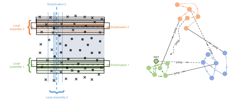
Figure 2: Example of cyclic AdaBoost iterations. This represents the toy problem defined in Eq. 83. The image row shows the decision stumps chosen by AdaBoost, the second image illustrate them in the space of decision stumps where the distance between the classifiers can be seen as the opposite of the similarity defined in Sec. 2.3.4.1.

This is illustrated in Fig. 2. More difficult problems don’t necessarily enlighten this phenomena this quickly, but we can still observe it in higher dimensions real-world problems.
The behavior that we tend to see is that in the first place, AdaBoost tries to cover a base space of estimators, and then, it seems to try to find the best combination of the estimators in this base space by repeating the same estimators over and over again but not necessarily as often as the others.

This intution has been formalized theoritically in the open problem presented in [39] in 2012, and this conjecture has very recently been proven in [3] in 2023. We will present the main ideas in the next subsubsection.

2.3.4.4 Theoritical insights

This subsubsection is based on [3]. This article proposes an original way to see AdaBoost. It is very formal, and we will try to keep most of their notations. Also, we volontary simplify the work they have done, which is way more riguourous and precise than this subsection. This subsection only stands to give intuitions of the results they have proven.
A dynamical system can be defined as follows:

Definition 2.3.7 (Dynamical system).

A dynamical system is a tuple $(\mathcal{X},\Sigma,\mu,f)$ where: • $\mathcal{X}$ is a compact metric space • $\Sigma$ is a $\sigma$-algebra on $\mathcal{X}$ • $\mu$ is a probability measure on $\mathcal{X}$ • $f$ is a measurable function from $\mathcal{X}$ to $\mathcal{X}$ which describes the evolution of the system

We will consider AdaBoost as a dynamical system over the weights of the data at each iteration. Thus, in our case, the dynamical system we consider is $(\Delta_{m},\Sigma_{m},\mu,\mathcal{A})$ where:

• $\Delta_{m}$ is the $m$-dimensional simplex, i.e. $\Delta_{m}=\{p\in\mathbb{R}^{m}|\sum_{i=1}^{m}p_{i}=1,p_{i}\geq 0\}$

• $\Sigma_{m}$ is the Borel $\sigma$-algebra on $\Delta_{m}$

• $\mu$ is a measure we will define later

• $\mathcal{A}$ is the AdaBoost update over the weights

The main goal of the paper is to be able to apply the Birkhoff Ergodic Theorem 2.3.8 [5] to the previous dynamical system.

Theorem 2.3.8 (Birkhoff Ergodic Theorem).

Let $(\mathcal{X},\Sigma,\mu,\mathcal{A})$ be a dynamical system and $f$ be a measurable function from $\mathcal{X}$ to $\mathbb{R}$. Then, there exists a measurable function $f^{*}$ such that: $$\lim_{n\to\infty}\frac{1}{T}\sum_{i=1}^{T}f(\mathcal{A}^{i}(x))=f^{*}(x)$$ (84) for $\mu$-almost every $x\in\mathcal{X}$. Also, we have that $f^{*}$ is $\mathcal{A}$-invariant, i.e. $f^{*}\circ\mathcal{A}=f^{*}$.

Applying this theorem to our dynamical system would allow us to prove the convergence of AdaBoost (w.r.t. the weights), and to prove that there exists a fixed point of the system.
To apply such theorem, we need to ensure that there exists a measure $\mu$ such that $\mathcal{A}$ is $\mu$-preserving. This is what the Krylov-Bogoliubov Theorem 2.3.9 states.

Theorem 2.3.9 (Krylov-Bogoliubov Theorem).

If $(W,N)$ is a metric compact space and $g:W\to W$ is a continuous function, then there exists a Borel probability measure $\mu$ on $W$ such that $g$ is $\mu$-preserving.

We now see that in order to apply the Birkhoff Ergodic Theorem, we only have to apply the Krylov-Bogoliubov Theorem to our (well-chosen) dynamical system. What we first can observe is that it is only relevant to set our first weight $w_{1}$ in the interior subset of the simplex $\Delta_{m}^{\circ}=\{w\in\mathbb{R}^{m}|\sum_{i=1}^{m}w_{i}=1,w_{i}>0\}$. Indeed, if we set $w_{1}$ to be $0$ for some $i$, then the weight will stay $0$ for all the iterations.
Let $\eta$ a dichotomy of the data, i.e. $\eta=(y_{1}h(x_{1}),\dots,y_{m}h(x_{m}))\in{\{-1,1\}}^{m}$ which is positive at the $i$th compenent only if $h$ classifies correctly sample $x_{i}$. We can define a set of weights $\pi(\eta):=\{w\in\Delta_{m},\eta\in\operatorname*{arg\,min}_{\eta^{\prime}}\eta^{\prime T}w\}$ the set of weights such that the estimator $h$ that minimizes the weighted error $w^{T}\eta_{h}$ verifies $\eta_{h}=\eta$.
Define also $\pi^{+}(\eta)=\{w\in\pi(\eta),\eta^{T}w>0\}$ the set of weights in $\pi(\eta)$ that are make non-zero error on mistake dichotomy $\eta$. Then, we can define $\Delta_{m}^{+}=\cup_{\eta\in{\{-1,1\}}^{m}}\pi^{+}(\eta)$ the set of weights that make non-zero error on at least one mistake dichotomy.
The first big result that is established in the paper is the following:

Proposition 2.3.10 (Continuity of AdaBoost Update).

The AdaBoost update $\mathcal{A}$ is continuous over the set $\cup_{\eta\in{\{-1,1\}}^{m}}\pi^{\circ}(\eta)$.

This is a key result to apply the Krylov-Bogoliubov Theorem.

[Proof.]Indeed, setting $w^{s}\to w$ a sequence of weights in $\cup_{\eta\in{\{-1,1\}}^{m}}\pi^{\circ}(\eta)$, we have that:

$$\mathcal{A}(w^{s})(i) =\frac{1}{2}w^{s}(i)\left(\frac{1}{\eta w^{s}}\right)^{\eta(i)}\left(\frac{1}{1-\eta w^{s}}\right)^{1-\eta(i)}$$ (85)

$$\underset{s\to\infty}{\to}\frac{1}{2}w(i)\left(\frac{1}{\eta w}\right)^{\eta(i)}\left(\frac{1}{1-\eta w}\right)^{1-\eta(i)}=\mathcal{A}(w)(i)$$

because $w^{s}\to w$ and $\eta w^{s}\to\eta w$. So we have that $\mathcal{A}(w^{s})\to\mathcal{A}(w)$, which proves the continuity of $\mathcal{A}$ over $\cup_{\eta\in\{-1,1\}^{m}}\pi^{\circ}(\eta)$. ∎ Their second main result is that the relative error of each weak classifier produced by AdaBoost can be lower bounded.

Proposition 2.3.11 (Lower bound on the relative error of weak classifiers).

$$\forall t\in\mathbb{N},w_{t}^{T}\eta_{h_{t}}\geq\frac{1}{2^{t+1}}$$ (86)

The proof is by induction, but is slightly more technical and needs to introduce more notations that we won’t detail here.
In [3], the authors don’t apply the Birkhoff Ergodic Theorem to the whole set $\Delta_{m}^{+}$, but only to a subset of it: the limit set of AdaBoost that can be reached by an infinite number of iterations starting from weights in $\Delta_{m}^{+}$ that they denote $\Omega_{\infty}^{+}=\cap_{t=1}^{\infty}\mathcal{A}^{t}(\Delta_{m}^{+})$.

Proposition 2.3.12 (Compactness of AdaBoost limit set).

$\Omega_{\infty}^{+}$ is compact.

The compactness of this set allows the authors to apply the Birkhoff Ergodic Theorem over $\Omega_{\infty}^{+}$. We thus have the following proposition:

Proposition 2.3.13 (AdaBoost is Ergodic over $\Omega_{\infty}^{+}$).

The average over any AdaBoost sequence starting at $w_{1}\in\Omega_{\infty}^{+}$ converges. More precisely, $$\forall w_{1}\in\Omega_{\infty}^{+},\forall f\in L^{1}(\mu),\frac{1}{T}\sum_{t=0}^{T-1}f(\mathcal{A}^{t}(w_{1}))\underset{T\to\infty}{\to}L(f)\in\mathbb{R}$$ (87)

Again, the proof is technical, and does not present much interest for our purpose. Finally, the authors show a last big result which they prove under different hypothesis. Here as well, we won’t go too much into the details here, but the theorem resembles to the following:

Theorem 2.3.14 (AdaBoost is Ergodic and Converges to a Cycle).

Let $\mathcal{A}^{\tau}$ a specific sequence of functions that converge towards the AdaBoost update $\mathcal{A}$ uniformly over $\Delta_{m}$. (In practice, those functions are explicit in the paper, and the author show the uniform convergence). Then, • $(w_{t})$ converges in finite time to a cycle in $\Delta_{m}^{+}$ of period $p$. • The AdaBoost system is ergodic. • Let $T_{0}$ be the first time at which $w_{t}$ enters the cycle. Then, for any $f\in L^{1}(\mu)$, we have that: $$\frac{1}{T}\sum_{t=0}^{T-1}f(\mathcal{A}^{t}(w_{1}))\underset{T\to\infty}{\to}\frac{1}{p}\sum_{t=0}^{p-1}f(\mathcal{A}^{T_{0}+t}(w_{1}))$$ (88)

That shows that after a high number of iterations, AdaBoost becomes perfectly cyclic. That confirms the intuition we can have Sec. 2.3.4.1.

However, this theorem is not completely satisfying. Indeed, this demonstrates that AdaBoost cycles w.r.t. the weights (thus w.r.t. the estimators $h$), but the cycle may be very long, and take a lot of iterations to be reached. In practice, we want to know if AdaBoost cycles w.r.t. the estimators $h$. The problem is that a cycle w.r.t. the estimators $h$ may not imply a cycle w.r.t. the weights. Indeed, the weights are not unique for a given estimator $h$. This is what motivated a discussion that we present in a future paper we will publish in a short time.

3 Conclusion & Acknowledgements

3.1 Conclusion

The primary objective of this paper has been to provide a comprehensive and expansive overview of AdaBoost, exploring the diverse interpretations and facets that extend beyond its initial introduction as a PAC learning algorithm. We have uncovered various ways to perceive and understand AdaBoost, highlighting the significance of comprehending each interpretation to attain a comprehensive understanding of the algorithm’s inner workings. In particular, the ergodic dynamics of AdaBoost have emerged as a compelling avenue of research, offering a new perspective that can foster theoretical advancements and shed light on its long-term behavior.

Although AdaBoost’s iterative dynamics are explicitly accessible at each step, comprehending its overall behavior on a global scale remains a challenging task. Consequently, studying the ergodic dynamics of AdaBoost has become an active and fruitful research domain for the past 30 years. By viewing AdaBoost as an ergodic dynamical system, novel theoretical frameworks and perspectives can be developed, enhancing our comprehension of its convergence properties, generalization bounds, and optimization landscape. This approach opens doors to explore the interplay between AdaBoost and related fields, such as deep learning, where phenomena like double descent have garnered significant attention.

Remarkably, the presence of a similar behavior to the double descent phenomenon was observed soon after AdaBoost’s introduction, yet it has not received extensive study except for a few notable papers. Given the recent surge of interest in double descent within the realm of deep learning, establishing connections and parallels between the dynamics of AdaBoost iterations and deep learning can significantly advance our understanding of both domains. By bridging these two fields of research, we can gain valuable insights into the intricate dynamics governing AdaBoost, leading to a deeper appreciation of its predictive power and potential applications.

This paper aims to serve various purposes for its readers. For those unfamiliar with AdaBoost, it offers a clear and concise introduction to the algorithm, elucidating its multiple interpretations and shedding light on its fundamental principles. By presenting the algorithm’s different perspectives in an accessible manner, readers can develop a solid foundation in AdaBoost and its significance within the broader machine learning landscape. Furthermore, experienced readers will find value in the paper’s ability to establish connections and unify diverse views of AdaBoost, presenting a cohesive and comprehensive understanding of the algorithm. This synthesis of perspectives provides a launching pad for future research endeavors centered around AdaBoost’s dynamics, enabling scholars to delve deeper into its behavior and explore novel research directions.

In conclusion, this paper has endeavored to provide a thorough exploration of AdaBoost, transcending its initial formulation as a PAC learning algorithm. By unifying the diverse interpretations and facets of AdaBoost, we have unveiled the intriguing concept of ergodic dynamics, which holds promise for advancing theoretical frameworks and deepening our comprehension of the algorithm’s behavior. We have also highlighted the significance of investigating the double descent phenomenon and establishing connections between AdaBoost other fields. By presenting AdaBoost in a multi-faceted manner, this paper caters to both novice and experienced readers, fostering a comprehensive understanding of the algorithm and paving the way for future research endeavors in AdaBoost’s dynamics and its broader implications in machine learning.

3.2 Acknowledgements

I would like to deeply thank Nicolas Vayatis and Argyris Kalogeratos for the time and effort they put in this project. I would also like to thank the IDAML Chair of Centre Borelli and its private partners for the funding of this project, without which this work would not have been possible.

Appendix A How to choose the base space of estimators?

From original to most modern versions of AdaBoost, it is always mentioned that AdaBoost, as any other boosting method, should be executed on a set of weak estimators. The definition of a weak estimator is not precise. In the original papers, boosting was considered as a PAC learning algorithm meaning that each estimator had at least a slightly better performance as a purely random estimator. Mathematically, this can write, for a classification problem with $K$ classes, as follows:
If the observation $x$ has the (true) label $k$, then there exists $\delta>0$ such that

$$\mathbb{P}(y=k|h(x)=k)\geq\mathbb{P}_{prior}(y=k)+\delta$$ (89)

where $\mathbb{P}_{prior}$ is a fixed prior that we chose according to our knowledge. For instance, we could fix $\mathbb{P}_{prior}(y=k)=\frac{\sum_{i=1}^{m}\mathbbm{1}_{y_{i}=k}}{m}$.

A.1 Too weak or too strong estimators

However, would boosting be relevant if our estimators were already strong in that sense? To properly see this, let’s take $\mathcal{H}_{d}(\mathcal{X})$ the set of decision trees of depth $d$ over the set $\mathcal{X}$. Suppose we have $m$ observations in $\mathcal{X}$. It is of course possible to build a tree $h\in\mathcal{H}_{m}(\mathcal{X})$ which achieves 100% accuracy on the set. Nonetheless, AdaBoost is not even designed to generate the next iteration of such classifier, as it is suppose to have an error $\epsilon>0$. But even considering decision trees of depth sufficiently small to ensure that none of them can classify the whole set, boosting can lose sense. Indeed, we can have two opposite phenomenas:

• Too weak estimators

• Too strong estimators

How can we have too weak estimators? Considering a classification task with $K>>2$ classes, we need to have complex enough weak estimators for boosting to properly work. If $\mathcal{H}_{1}(\mathcal{X})$ is our set of weak estimators, each of the tree of this set will achieve a very low accuracy, and probably way less than any random guesser if the data is complex enough to be non-linearly seperable for instance.

Now, we can have estimators that are too strong as well. Indeed, if each of the tree in the boosting sequence achieves an accuracy which is close to perfect accuracy, the benefits from boosting methods vanish automatically. Of course, it still depends on what you aim for in your problem, but using a boosting method to fit $100$ trees of depth $10$ on a complex task can require much more time than training a single strong classifier. Plus, this will not likely prevent overfitting as the sequence of decision trees will not vary a lot (because each tree achieves very satisfying accuracy on the train set), meaning that the boosting classifier will truly use only a few different decision trees when you expect it to use tens or hundreds different ones to aggregate the result.

A.2 How to detect too good or too weak estimators?

The easier to detect is when your estimator are too strong. It is also probably the one that is the most likely to happen. Indeed, in that case, you can observe several things running boosting:

• Each one of the estimator in the sequence achieves high accuracy on the train set.

• The similarity between the estimators is too high.

• The difference between the precision of each estimator and the precision of the aggregated estimator is small.

Let’s take an example here. Consider the Fashion MNIST dataset. We consider several sets of estimators: $\mathcal{H}_{1}(\mathcal{X}),\dots,\mathcal{H}_{15}(\mathcal{X})$. For each depth, we run AdaBoost for $T=\{10,20,\dots,100\}$ iterations. We then compare the difference between the mean accuracy of each decision tree and the ensemble model. Also, we compute the similarity between each estimator of the sequence.

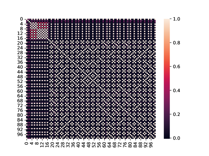
Figure 3: Similarity matrix for depth $1$. In $(i,j)$, the similarity measure between classifier $i$ and $j$ measured by kappa statistic. We recognize here the cyclic patterns due to the lack of complexity of our set of estimators.

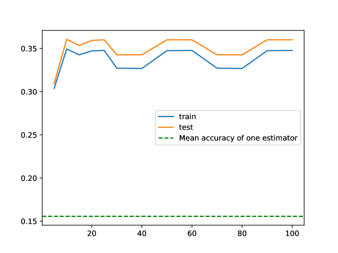
Figure 4: Accuracy for depth $1$. On the $x$-axis, the number of estimators kept to build the ensemble, and on the $y$-axis, the accuracy of the considered estimator.

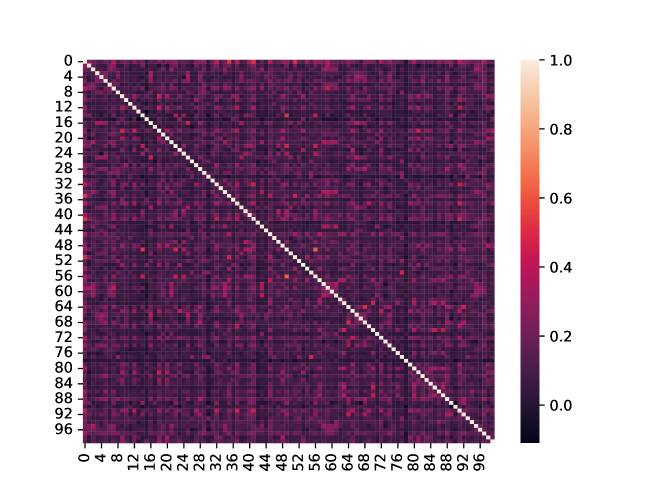
Figure 5: Similarity matrix for depth $4$. In $(i,j)$, the similarity measure between classifier $i$ and $j$ measured by kappa statistic. Here, the produced sequence is very diverse and all estimators are sufficiently different from each other to have a true benefit from boosting.

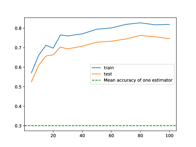
Figure 6: Accuracy for depth $4$. On the $x$-axis, the number of estimators kept to build the ensemble, and on the $y$-axis, the accuracy of the considered estimator.

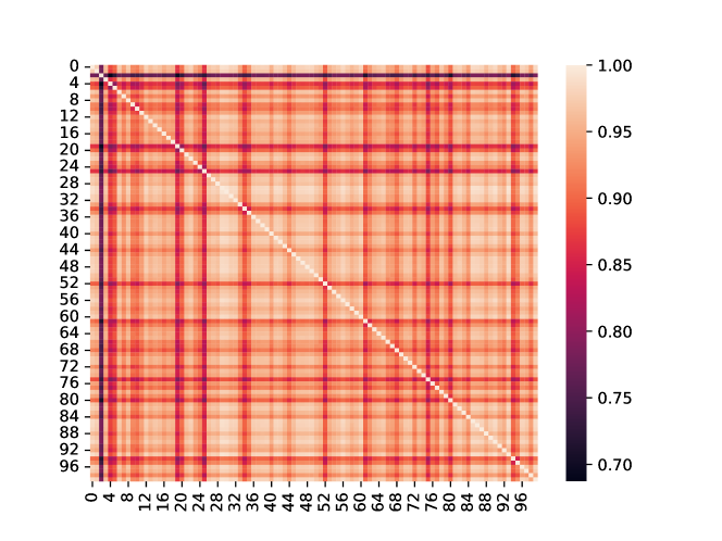
Figure 7: Similarity matrix for depth $15$. In $(i,j)$, the similarity measure between classifier $i$ and $j$ measured by kappa statistic. As we can see, the similarity is very high between each estimator, meaning that the boosting sequence is not diverse enough because the estimators are too strong.

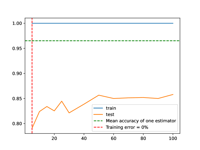
Figure 8: Accuracy for depth $15$. On the $x$-axis, the number of estimators kept to build the ensemble, and on the $y$-axis, the accuracy of the considered estimator.

On the Fig. 3, 4, 5, 6, 7, 8, 9, we see that if we take a depth of $1$, the estimators are too weak and we cannot learn properly as the algorithm stucks itself in a cycle to quickly. However, we have the opposite with depth $15$ for which boosting seems quite useless, and all estimators seem to be the same. A good set of classifiers here is thus trees of depth $4$ or $5$, for example. We can also observe that the more more complex the set of estimator is, the more similar the sequence of estimator is.

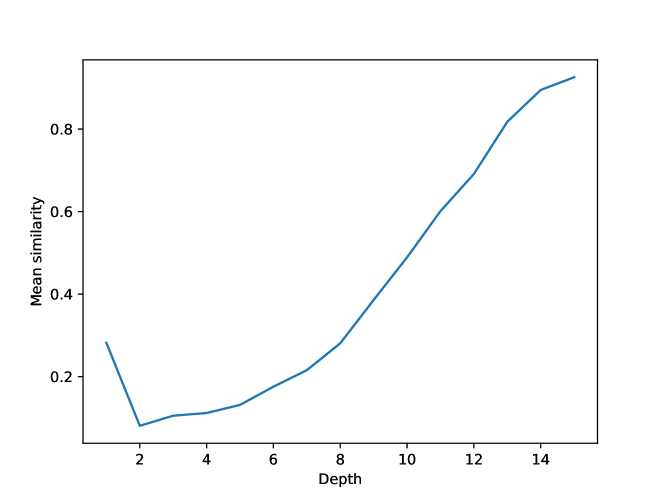
Figure 9: Mean similarity inside the sequence of estimators. We notice that the more complex the set of estimator is, the more similar the sequence of estimators become.

References

- [1] Aleksandr Y Aravkin, Giulio Bottegal and Gianluigi Pillonetto “Boosting as a kernel-based method” In Machine Learning 108.11 Springer, 2019, pp. 1951–1974
- [2] Peter Bartlett, Yoav Freund, Wee Sun Lee and Robert E Schapire “Boosting the margin: A new explanation for the effectiveness of voting methods” In The annals of statistics 26.5 Institute of Mathematical Statistics, 1998, pp. 1651–1686
- [3] Joshua Belanich and Luis E Ortiz “On the convergence properties of optimal AdaBoost” In arXiv preprint arXiv:1212.1108, 2023
- [4] Candice Bentejac, Anna Csorgo and Gonzalo Martinez-Munoz “A comparative analysis of gradient boosting algorithms” In Artificial Intelligence Review 54 Springer, 2021, pp. 1937–1967
- [5] George D Birkhoff “Proof of the ergodic theorem” In Proceedings of the National Academy of Sciences 17.12 National Acad Sciences, 1931, pp. 656–660
- [6] Hongming Chen et al. “The rise of deep learning in drug discovery” In Drug discovery today 23.6 Elsevier, 2018, pp. 1241–1250
- [7] Tianqi Chen and Carlos Guestrin “Xgboost: A scalable tree boosting system” In Proceedings of the 22nd acm sigkdd international conference on knowledge discovery and data mining, 2016, pp. 785–794
- [8] Joseph A Cruz and David S Wishart “Applications of machine learning in cancer prediction and prognosis” In Cancer informatics 2 SAGE Publications Sage UK: London, England, 2006, pp. 117693510600200030
- [9] Robert Culkin and Sanjiv R Das “Machine learning in finance: the case of deep learning for option pricing” In Journal of Investment Management 15.4, 2017, pp. 92–100
- [10] Sukhpreet Singh Dhaliwal, Abdullah-Al Nahid and Robert Abbas “Effective intrusion detection system using XGBoost” In Information 9.7 MDPI, 2018, pp. 149
- [11] Thomas G Dietterich “Ensemble methods in machine learning” In Multiple Classifier Systems: First International Workshop, MCS 2000 Cagliari, Italy, June 21–23, 2000 Proceedings 1, 2000, pp. 1–15 Springer
- [12] Matthew F Dixon, Igor Halperin and Paul Bilokon “Machine learning in Finance” Springer, 2020
- [13] Narayanan U Edakunni, Gary Brown and Tim Kovacs “Boosting as a product of experts” In arXiv preprint arXiv:1202.3716, 2012
- [14] Sophie Emerson, Ruairí Kennedy, Luke O’Shea and John O’Brien “Trends and applications of machine learning in quantitative finance” In 8th international conference on economics and finance research (ICEFR 2019), 2019
- [15] Ky Fan “Minimax theorems” In Proceedings of the National Academy of Sciences 39.1 National Acad Sciences, 1953, pp. 42–47
- [16] Robert M. Freund, Paul Grigas and Rahul Mazumder “AdaBoost and Forward Stagewise Regression are First-Order Convex Optimization Methods” arXiv:1307.1192 [cs, math, stat] arXiv, 2013 URL: http://arxiv.org/abs/1307.1192
- [17] Yoav Freund “Boosting a weak learning algorithm by majority” In Information and computation 121.2 Elsevier, 1995, pp. 256–285
- [18] Yoav Freund and Robert E Schapire “A Decision-Theoretic Generalization of On-Line Learning and an Application to Boosting” In Journal of Computer and System Sciences 55.1, 1997, pp. 119–139 DOI: 10.1006/jcss.1997.1504
- [19] Yoav Freund and Robert E Schapire “Experiments with a new boosting algorithm” In icml 96, 1996, pp. 148–156 Citeseer
- [20] Jerome Friedman, Trevor Hastie and Robert Tibshirani “Additive logistic regression: a statistical view of boosting (with discussion and a rejoinder by the authors)” In The annals of statistics 28.2 Institute of Mathematical Statistics, 2000, pp. 337–407
- [21] Jerome H Friedman “Stochastic gradient boosting” In Computational statistics & data analysis 38.4 Elsevier, 2002, pp. 367–378
- [22] Jerome H Friedman and Werner Stuetzle “Projection pursuit regression” In Journal of the American statistical Association 76.376 Taylor & Francis, 1981, pp. 817–823
- [23] Periklis Gogas and Theophilos Papadimitriou “Machine learning in economics and finance” In Computational Economics 57 Springer, 2021, pp. 1–4
- [24] Margherita Grandini, Enrico Bagli and Giorgio Visani “Metrics for multi-class classification: an overview” In arXiv preprint arXiv:2008.05756, 2020
- [25] Michael I Jordan and Tom M Mitchell “Machine learning: Trends, perspectives, and prospects” In Science 349.6245 American Association for the Advancement of Science, 2015, pp. 255–260
- [26] Guolin Ke et al. “Lightgbm: A highly efficient gradient boosting decision tree” In Advances in neural information processing systems 30, 2017
- [27] B Ravi Kiran et al. “Deep reinforcement learning for autonomous driving: A survey” In IEEE Transactions on Intelligent Transportation Systems 23.6 IEEE, 2021, pp. 4909–4926
- [28] Jyrki Kivinen and Manfred K. Warmuth “Boosting as entropy projection” In Proceedings of the twelfth annual conference on Computational learning theory Santa Cruz California USA: ACM, 1999, pp. 134–144 DOI: 10.1145/307400.307424
- [29] Yann LeCun, Yoshua Bengio and Geoffrey Hinton “Deep learning” In nature 521.7553 Nature Publishing Group UK London, 2015, pp. 436–444
- [30] Nan Li, Yang Yu and Zhi-Hua Zhou “Diversity Regularized Ensemble Pruning.” In ECML/PKDD (1), 2012, pp. 330–345
- [31] Tengyuan Liang and Benjamin Recht “Interpolating classifiers make few mistakes” In arXiv preprint arXiv:2101.11815, 2021
- [32] Llew Mason, Jonathan Baxter, Peter Bartlett and Marcus Frean “Boosting algorithms as gradient descent” In Advances in neural information processing systems 12, 1999
- [33] Sajjad Mozaffari et al. “Deep learning-based vehicle behavior prediction for autonomous driving applications: A review” In IEEE Transactions on Intelligent Transportation Systems 23.1 IEEE, 2020, pp. 33–47
- [34] Preetum Nakkiran et al. “Deep double descent: Where bigger models and more data hurt” In Journal of Statistical Mechanics: Theory and Experiment 2021.12 IOP Publishing, 2021, pp. 124003
- [35] Alexey Natekin and Alois Knoll “Gradient boosting machines, a tutorial” In Frontiers in neurorobotics 7 Frontiers Media SA, 2013, pp. 21
- [36] Adeola Ogunleye and Qing-Guo Wang “XGBoost model for chronic kidney disease diagnosis” In IEEE/ACM transactions on computational biology and bioinformatics 17.6 IEEE, 2019, pp. 2131–2140
- [37] Saharon Rosset, Ji Zhu and Trevor Hastie “Boosting as a Regularized Path to a Maximum Margin Classifier”
- [38] Cynthia Rudin, Ingrid Daubechies and Robert E Schapire “The Dynamics of AdaBoost: Cyclic Behavior and Convergence of Margins”
- [39] Cynthia Rudin, Robert E Schapire and Ingrid Daubechies “Open Problem: Does AdaBoost Always Cycle?” In Conference on Learning Theory, 2012, pp. 46–1 JMLR WorkshopConference Proceedings
- [40] Cynthia Rudin, Ingrid Daubechies, Robert E Schapire and Dana Ron “The dynamics of AdaBoost: cyclic behavior and convergence of margins.” In Journal of Machine Learning Research 5.10, 2004
- [41] Omer Sagi and Lior Rokach “Ensemble learning: A survey” In Wiley Interdisciplinary Reviews: Data Mining and Knowledge Discovery 8.4 Wiley Online Library, 2018, pp. e1249
- [42] Robert E Schapire “The boosting approach to machine learning: An overview” In Nonlinear estimation and classification Springer, 2003, pp. 149–171
- [43] Robert E Schapire “The strength of weak learnability” In Machine learning 5 Springer, 1990, pp. 197–227
- [44] Robert E Schapire and Yoav Freund “Boosting: Foundations and algorithms” In Kybernetes 42.1 Emerald Group Publishing Limited, 2013, pp. 164–166
- [45] Brent Smith and Greg Linden “Two decades of recommender systems at Amazon. com” In Ieee internet computing 21.3 Ieee, 2017, pp. 12–18
- [46] Harald Steck et al. “Deep learning for recommender systems: A Netflix case study” In AI Magazine 42.3, 2021, pp. 7–18
- [47] Xiaolei Sun, Mingxi Liu and Zeqian Sima “A novel cryptocurrency price trend forecasting model based on LightGBM” In Finance Research Letters 32 Elsevier, 2020, pp. 101084
- [48] Ayşegül Uçar, Yakup Demir and Cüneyt Güzeliş “Object recognition and detection with deep learning for autonomous driving applications” In Simulation 93.9 SAGE Publications Sage UK: London, England, 2017, pp. 759–769
- [49] Jessica Vamathevan et al. “Applications of machine learning in drug discovery and development” In Nature reviews Drug discovery 18.6 Nature Publishing Group UK London, 2019, pp. 463–477
- [50] Dehua Wang, Yang Zhang and Yi Zhao “LightGBM: an effective miRNA classification method in breast cancer patients” In Proceedings of the 2017 international conference on computational biology and bioinformatics, 2017, pp. 7–11
- [51] Jian Wei et al. “Collaborative filtering and deep learning based recommendation system for cold start items” In Expert Systems with Applications 69 Elsevier, 2017, pp. 29–39
- [52] Abraham J Wyner, Matthew Olson, Justin Bleich and David Mease “Explaining the success of adaboost and random forests as interpolating classifiers” In The Journal of Machine Learning Research 18.1 JMLR. org, 2017, pp. 1558–1590
- [53] Zhi-Hua Zhou “Ensemble methods” In Combining pattern classifiers. Wiley, Hoboken, 2014, pp. 186–229