Mass gaps of a $\mathbb{Z}_{3}$ gauge theory with three fermion flavors in $1+1$ dimensions

Abstract

We consider a $\mathbb{Z}_{3}$ gauge theory coupled to three degenerate massive flavors of fermions, which we term “QZD”. The spectrum can be computed in $1+1$ dimensions using tensor networks. In weak coupling the spectrum is that of the expected mesons and baryons, although the corrections in weak coupling are nontrivial, analogous to those of non-relativistic QED in $1+1$ dimensions. In strong coupling, besides the usual baryon, the singlet meson is a baryon anti-baryon state. For two special values of the coupling constant, the lightest baryon is degenerate with the lightest octet meson, and the lightest singlet meson, respectively.

I Introduction

How confinement in gauge theories produces a non-trivial mass spectrum is a problem of fundamental importance for a wide variety of problems, from Quantum ChromoDynamics (QCD) in the strong interactions Wilson (1974); Kogut and Susskind (1974), to numerous systems in condensed matter Fradkin (2013).

The simplest examples of confining gauge theories are of course in the fewest number of spacetime dimensions, which is $1+1$. The iconic examples are fermions coupled to an Abelian gauge theory, which is the Schwinger model Schwinger (1962); Banks et al. (1976); Coleman et al. (1975); Coleman (1976); Manton (1985) and $N_{f}$ flavors of quarks coupled to a ${\rm SU}(N_{c})$ non-Abelian gauge theory, with $N_{c}$ the number of colors. For $N_{f}\ll N_{c}\rightarrow\infty$, this is the ’t Hooft model ’t Hooft (1974); Callan et al. (1976); Fonseca and Zamolodchikov (2006); Fateev et al. (2009); Ziyatdinov (2010); Zubov et al. (2015).

As an Abelian theory the Schwinger model is especially useful. For a single, massless fermion, Schwinger showed that the only gauge invariant state is a single free, massive boson Schwinger (1962). When the fermions are massive, however, there is an infinite number of gauge invariant pairs of fermions and anti-fermions. These obviously do not carry fermion number, and are a type of meson. When their mass is large, Coleman computed the number of mesons semi-classically Coleman (1976).

While classical computers can be used to numerically compute many properties of field theories, there are some aspects — notably the evolution in real time, or theories with a sign problem — for which quantum computers are necessary. This requires controlling the Hilbert space of a field theory, which even with a lattice regularization is exponentially large. In $1+1$ dimensions though, polynomial approximations have been developed, as matrix product states (MPS) efficiently represent the ground states of gapped systems Buyens et al. (2014); Bañuls et al. (2013); Cirac et al. (2021). Studies of the Schwinger model on quantum computers include Refs. Hauke et al. (2013); Rico et al. (2014); Pichler et al. (2016); Zohar et al. (2016); Martinez et al. (2016); Muschik et al. (2017); Klco et al. (2018); Bañuls et al. (2020); Surace et al. (2020); Bañuls and Cichy (2020); Yang et al. (2020). Other properties analyzed include how mesons scatter Rigobello et al. (2021, 2023), thermalization Desaules et al. (2023); Chanda et al. (2020), string breaking Pichler et al. (2016); Kühn et al. (2015); Magnifico et al. (2020); de Jong et al. (2022); Lee et al. (2023), entanglement production in jets Florio et al. (2023) and the dynamics in $\theta$-vacuum Zache et al. (2019); Kharzeev and Kikuchi (2020); Ikeda et al. (2021).

In the massive Schwinger model the only states which survive confinement are mesons. It would be useful to study models where confinement produces states which do carry net fermion number, analogous to baryons in QCD.

There are several such models in $1+1$ dimensions. As a ${\rm SU}(N_{c})$ gauge theory, the ’t Hooft model has baryons, but their properties are opaque Witten (1979); Steinhardt (1980); Bringoltz (2009). A ${\rm SU}(N_{c})$ gauge theory coupled to $N_{f}$ light flavors of quarks can be analyzed using conformal field theory, as a type of Wess-Zumino-Novikov-Witten model Lajer et al. (2022); it behaves in a manner characteristic of such two dimensional theories. Rico et al. Rico et al. (2018) studied a ${\rm SO}(3)$ model in which both the quarks and the gluons lie in the adjoint representation, and so a quark and a gluon can directly combine to form a gauge invariant fermion. This is like a ${\rm SU}(N_{c})$ gauge theory coupled to quarks in the adjoint representation, instead of the fundamental representation as in QCD. Lastly, Farrell et al. Farrell et al. (2023) directly integrated out the ${\rm SU}(N_{c})$ gauge fields, which is possible in $1+1$ dimensions, to obtain the mass spectrum for ${\rm SU}(3)$ gauge fields coupled to two massive flavors.

While these models are all useful, we wish to study a simpler model where fermions emerge as gauge invariant states. Before doing so, it is necessary to explain in detail why in the Schwinger model, a single, massive flavor has no gauge invariant states with net fermion number. In Minkowski spacetime, the total Hamiltonian is

$$H=\int\mathrm{d}x\left[\overline{\psi}\left(-i\gamma^{1}\partial_{1}+\gamma^{1}A_{1}+m\right)\psi\right]+\tfrac{g^{2}}{2}E^{2}\ ,$$ (1)

where $E$ is the electric field operator, and $A_{1}$ the conjugate gauge potential. Gauge invariance requires that we impose Gauss’s law,

$$\partial_{1}E=\overline{\psi}\gamma^{0}\psi\ .$$ (2)

The right hand side is just the charge density for the fermion field, which for a single flavor, is identical to the density for fermion number. (To represent Wilson loops it is necessary to add an external charge density to the right hand side, which manifestly extends the Hilbert space Gervais and Sakita (1978); Pisarski (2022); Kaplan et al. (2023).) Computing the total electric charge, $Q_{\rm tot}$, Gauss’s law gives

$$Q_{\rm tot}=\int\mathrm{d}x\,\partial_{1}E=E(\infty)-E(-\infty)\ .$$ (3)

For the system to be well defined in the limit of infinite volume, we require that there is no net electric field, $E(\infty)=E(-\infty)$, and the total electric charge vanishes, $Q_{\rm tot}=0$ Further, since for a single flavor the total fermion number equals the total charge $N_{\rm tot}=0$ as well, where by $N$ we mean the number of particles relative to half-filling, or equivalently, relative to the ground state.

Thus in a ${\rm U}(1)$ theory in $1+1$ dimensions, for a single flavor Gauss’s law prevents us from introducing any net fermion number. In short, the global ${\rm U}(1)$ symmetry of fermion number is already part of the ${\rm U}(1)$ gauge symmetry.

This can be seen explicitly by trying to introduce a chemical potential for fermion number, $\mu$. In the Hamiltonian formalism all thermodynamics quantities follow from the partition function,

$$Z(T,\mu)=\mathrm{Tr}\left(e^{-(H-\mu N_{\rm tot})/T}\right)\;,$$ (4)

where the trace is over all physical states. Physical states, though, must obey Gauss’s law. For ${\rm U}(1)$, this enforces $Q_{\rm tot}=N_{\rm tot}=0$, and consequently, that the partition function is independent of $\mu$, $Z(T,\mu)=Z(T,0)$.

This is can also be seen directly using the Lagrangian formalism. For a single flavor, $\mu\neq 0$ can be eliminated simply by shifting the time like component of the vector potential by an imaginary constant, $A_{0}\rightarrow A_{0}-i\mu/g$ Dumitru et al. (2005).

With two or more flavors, then clearly one can introduce a fermion number for one flavor relative to those for the others. This is evident for two flavors, which we call up, $u$, and down, $d$. Then a net electric charge from an excess of $u$ fermions over $u$ anti-fermions can be precisely cancelled by an excess of down anti-fermions, $\overline{d}$, over $d$ fermions. This is obviously just a chemical potential for isospin between the up and down quarks. While an isospin chemical potential exhibits interesting phenomena, such as spatially varying phases Narayanan (2012); Lohmayer and Narayanan (2013); Bañuls et al. (2017), it still leaves us bereft of gauge invariant fermions.

A simple model where there are both gauge invariant fermions and bosons was proposed in Ref. Pisarski (2021). Consider a $\mathbb{Z}_{3}$ gauge theory coupled to three, degenerate massive flavors of fermions, adding strange, $s$, to $u$ and $d$. By the Fermi exclusion principle, we cannot put two identical fermions at the same point in space, since $u^{2}=0$, etc. This is unlike QCD, where three quarks of the same flavor can sit on the same point in space, as long as they each carry a different color; for example, in QCD the $\Omega$ baryon is $sss$. Assuming that the $\mathbb{Z}_{3}$ gauge theory confines, the only way to put fermions at the same point in space is if they have different flavors. Thus the simplest singlet under the $\mathbb{Z}_{3}$ gauge group is $uds$, which is like the $\Lambda$ baryon in QCD.

Confinement also produces mesons in this $\mathbb{Z}_{3}^{\;3}$ theory, but these are simple to understand. Since there are three degenerate flavors, we can form $\mathbb{Z}_{3}$ singlets in two ways. There is a flavor singlet,

$$\eta^{\prime}=\sum_{f=1}^{3}\overline{\psi}^{f}\psi^{f}\ ,$$ (5)

and a flavor octet,

$$\pi^{A}=\sum_{f,g=1}^{3}\overline{\psi}^{f}t^{A}_{fg}\,\psi^{g}\ ;$$ (6)

$f$ and $g$ are indices for the fundamental representation of flavor, $f,g=1,2,3$, while $t^{A}_{fg}$ is a ${\rm SU}(3)$ flavor matrix in the adjoint representation, $A=1\ldots 8$. As suggested by the notation, the singlet meson is like the $\eta^{\prime}$ meson in QCD, while the octet multiplet $\pi^{A}$ is analogous to the $\pi$, $K$, and $\eta$ mesons.

Thus we have a model which has gauge invariant singlets which are both fermions (baryons) and bosons (mesons). To avoid the the subtleties and complications of chiral symmetry breaking in two spacetime dimensions, we take the fermions to all have the same, nonzero mass.

In this paper we study the mass spectrum of the lightest states of this $\mathbb{Z}_{3}^{\;3}$ theory as a function of the coupling constant on the lattice. First we discuss the theory on a lattice, and how to obtain a $\mathbb{Z}_{3}$ gauge theory from the spontaneous breaking of a ${\rm U}(1)$ gauge theory. Tensor networks Weichselbaum (2012a); Orus (2014); Fishman et al. (2020); Meurice et al. (2022) and the Density Matrix Renormalization Group (DMRG) are then used to compute the mass spectrum. We find that QZD exhibits a fascinating and unexpected relation between the masses of the lightest fermions and bosons.

All states measured are gauge invariant, and so confined. This is encouraging, as there is a long history suggesting that confinement in both $2+1$ and $3+1$ dimensions are dominated by the $\mathbb{Z}_{3}$ vortices of ${\rm SU}(3)$ gauge theories Greensite (2017); Sale et al. (2023); Biddle et al. (2022a, b, 2023). In $1+1$ dimensions, these $\mathbb{Z}_{3}$ vortices are points in spacetime, but should also confine.

II QZD and its weak and strong coupling limit

Our starting point will be the following standard lattice Hamiltonian

$$H_{L}\! = \!-\tfrac{i}{2a}\sum_{x=1}^{L-1}\bigl{(}U_{x}^{\dagger}\,\boldsymbol{\chi}^{\dagger}_{x}\cdot\boldsymbol{\chi}_{x+1}{-}\mathrm{H.c.}\bigr{)}-m\sum_{x=1}^{L}(-1)^{x}{n_{x}}$$ (7)

$$+\tfrac{ag^{2}}{2}\sum_{x=1}^{L-1}E_{x}^{2}\text{ ,}$$

where $\boldsymbol{\chi}_{x}{\equiv}(\chi_{1},\ldots,\chi_{N_{f}})_{x}^{T}$ are staggered fermions of $N_{f}$ flavors that live on even/odd sites representing the original left/right chiralities. The particle number at a site

$$n_{x}\equiv\boldsymbol{\chi}_{x}^{\dagger}\cdot\boldsymbol{\chi}_{x}\equiv\sum_{f=1}^{N_{f}}\chi_{x}^{f\dagger}\chi_{x^{\prime}}^{f}\text{ ,}$$ (8)

includes a symmetric sum over all flavors. It follows from Eq. (7), that like $E_{x}$, $U_{x}$ lives on the bond in between sites $x$ and $x+1$. We consider a finite system with a total of $L$ sites together with open boundary conditions (BC). The unit of energy is assumed in terms of the hopping amplitude $1/(2a):=1$, i.e., $a=1/2$, unless specified otherwise. For the remainder of the paper, we focus on the case of $N_{f}=3$ fermionic flavors.

The model differs from the Schwinger model in that $U_{x}$, $E_{x}$ and Gauss law implement a local $\mathbb{Z}_{3}$ algebra Horn et al. (1979); Kogut et al. (1980); Kogut (1980); Alcaraz and Koberle (1981, 1980); Zohar et al. (2017); Ercolessi et al. (2018); Magnifico et al. (2019a, b); Borla et al. (2020); Frank et al. (2020); Emonts et al. (2020); Robaina et al. (2021); Emonts et al. (2023). Defining the operator

$$P_{x} \equiv \exp\left(\tfrac{2\pi i}{3}\;E_{x}\right)$$ (9)

we impose

$$P_{x}^{3}=U_{x}^{3}=1\ ;\quad P_{x}^{\dagger}P_{x}^{\,}=U_{x}^{\dagger}U_{x}^{\,}=1$$ (10)

$$U_{x}P_{x}={\rm e}^{2\pi i/3}P_{x}U_{x}\ .$$ (11)

In the basis where the electric field is diagonal, $U_{x}$ takes the role of a cyclic permutation operator,

$$U_{x}=\begin{pmatrix}0&1&0\\ 0&0&1\\ 1&0&0\end{pmatrix}\ ,$$ (12)

that increments (or for $U^{\dagger}$ decrements the gauge field. This is supplemented by a $\mathbb{Z}_{3}$ Gauss law

$$P_{{x}}^{\,}P_{{x-1}}^{\dagger}=\exp\left(\tfrac{2\pi i}{3}\,q_{x}\right)\ .$$ (13)

with the charge density defined as usual for staggered fermions

$$q_{x}=\left\{\begin{array}[c]{ll}n_{x}&\text{for }x\text{ odd}\\ n_{x}-N_{f}&\text{for }x\text{ even }\ (N_{f}=3)\ .\end{array}\right.$$ (16)

This permits the simple interpretation that odd sites behave like ‘particles’ which carry electrical charge $+1$, thus having $q_{x}=(+1)\,n_{x}$, whereas even sites behave like ‘holes’, carrying electrical charge $-1$ for every hole relative to completely filled, thus having $q_{x}=(-1)\,(N_{f}-n_{x})=n_{x}-N_{f}$.

While the variables are similar to the implementation of a ${\rm U}(1)$ gauge theory by quantum links Chandrasekharan and Wiese (1997); Brower et al. (1999), Gauss’ law is different, as the flux is only conserved modulo 3. We further massage Eq. (7) to make it more amenable to numerical simulations. We start by imposing open boundary conditions on our chain $E_{0}=E_{L}=\chi_{L+1}=0$. This allows us to use the remaining gauge transformations to remove the links $U_{x}$ from the theory (see for instance Ref. Chakraborty et al. (2022)) and solve Gauss’ law, expressing the electric field operators in terms of the fermionic fields. We have

$$E_{x} =\left(Q_{x}\,{\rm mod}\,3\right)$$ (17)

with the cumulative charge

$$Q_{x} \equiv\sum_{{x^{\prime}\leq x}}{q_{x^{\prime}}}\ ,$$ (18)

and where modulo is taken symmetric around zero, i.e., having $E_{x}\in\{-1,0,1\}$. Thus in $1+1$ dimensions the gauge fields are not dynamical, as they can be completely determined by the charge configuration. This permits one to express a long-range Hamiltonian entirely in terms of the fermion fields. By exploiting Abelian ${\rm U}(1)$ particle number symmetry in the simulation, this is conveniently done relative to half-filling all along. With this then the symmetry label for the cumulative block particle number

$$N_{x} \equiv\sum_{{x^{\prime}\leq x}}({n_{x^{\prime}}-n_{0}})\ ,$$ (19)

with $n_{0}=N_{f}/2$ the average half-filling directly specifies $Q_{x}$ for even block size, i.e., $Q_{x}=N_{x}$. For odd block size this requires a minor tweak based on Eq. (16) ensuring that $Q_{x}\in\mathbb{Z}$.

A continuum form of a $\mathbb{Z}_{3}$ gauge theory can be constructed following Krauss, Preskill, and Wilczek Krauss and Wilczek (1989); Preskill and Krauss (1990); Pisarski (2021). One begins with a ${\rm U}(1)$ gauge field, coupled to fermions with unit charge, and a scalar field, $\phi$, not with unit charge, but with charge three. Arranging the potential for the scalar field to develop an expectation value in vacuum, $\phi_{0}$, the photon develops a mass $m_{\gamma}=3g\phi_{0}$, and so is screened over distances $>1/m_{\gamma}$. Since the scalar field has charge three, the $\phi$ field is insensitive to the presence of $\mathbb{Z}_{3}$ vortices, which leaves a local $\mathbb{Z}_{3}$ symmetry, at least over distances $>1/m_{\gamma}$. Remember that a scalar field has zero mass dimension in two dimensions, so by taking $\phi_{0}\gg 1$, the ${\rm U}(1)$ photon is very heavy, and the theory only goes from the effective $\mathbb{Z}_{3}$ gauge symmetry, to the full ${\rm U}(1)$, at short distances $\leq 1/m_{\gamma}$.

Symmetries

The states in the theory can be labeled by their total particle number $N_{\rm tot}$ which we take relative to half-filling for convenience, and the representation of ${\rm SU}(3)_{f}$ flavor symmetry $(n_{s},n_{a})$ to which they belong. Here $n_{s}$/$n_{a}$ denote the symmetric/antisymmetric rank of the representation. We then use $(N_{\rm tot};n_{s}n_{a})$ as a compact notation to label all symmetry sectors, as explained in App. B. We restrict ourselves to the ground state sector $(0;00)$, and the lightest states $(0;11),(3;00),(3;11)$. Here $(11)\equiv{\bf 8}$ (octet) specifies the adjoint representation of ${\rm SU}(3)$. Mesons live in the $N_{\rm tot}=0$ sector, while baryons live in the $N_{\rm tot}=3$ sector. As explained in the Introduction, this is unlike a ${\rm U}(1)$ theory, since both sectors can be realized in the absence of any net external charge, i.e. in the gauge invariant sector which satisfies Gauss’s law. The ground state in the $(0;00)$ sector represents the QZD vacuum, with no baryon or meson excitations present.

III Results

III.1 Weak coupling regime

Naively, one might expect that the weak coupling behavior of this theory would be the usual power series in $g^{2}$. To understand why this is not so, start first with the case of a ${\rm U}(1)$ gauge theory in two spacetime dimensions. In the continuum, the Coulomb potential is

$$V(x)=g^{2}\int dk\,\frac{{\rm e}^{ikx}}{k^{2}}\sim g^{2}|x|\,$$ (20)

is confining. For very small coupling, the fermions are heavy, and we should be able to use a non-relativistic approximation:

$${\cal H}_{\rm non-rel}=-\frac{1}{2m}\frac{d^{2}}{dx^{2}}+g^{2}\frac{|x|}{4}\,\;.$$ (21)

Because this is a confining potential, the weak coupling expansion is not a power series in $g^{2}/m^{2}$, but in $(g^{2}/m^{2})^{1/3}$ Fonseca and Zamolodchikov (2006); Fateev et al. (2009); Ziyatdinov (2010); Zubov et al. (2015). In App. A we show that the meson mass behaves as

$$\frac{M_{\rm meson}}{m}=2m\cdot\left(1+0.40431\cdot\left(\frac{g}{2m}\right)^{4/3}+O\left(\frac{g^{2}}{m^{2}}\right)\right)$$ (22)

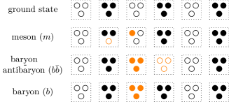
Figure 1: Illustration of the strong coupling limit. The ground state (top row) corresponds to half-filling. The first excitation is a single baryon (last row). We highlight in orange the deviation from the ground state. The first “mesonic” state is a baryon-antibaryon pair which in QZD does not generate an electric field (by contrast, a single meson requires partial fillings; since necessarily also delocalized, by Gauss law this will always generate electric field, and hence decouple at strong coupling to large energies).

III.2 Strong coupling regime

Another limit that is under control is the strong coupling region of the lattice model, keeping the lattice spacing $a$ fixed as $g\to\infty$). The vacuum at infinite coupling is elementary, and direct to expand about. In terms of spins, it corresponds to half-filling: for each flavor, all even sites are occupied, while all odd sites are empty, as in Fig. 1. The first excitation is a “baryon”, with one fermion of each flavor sitting at the same site. Thanks to the periodicity of Gauss’s law for $\mathbb{Z}_{3}$, such a configuration has zero net charge. Thus to zeroth order in $1/g$, the mass of the baryon is just $3m$, see (Fig. 2 below). The leading correction in $1/g^{2}$ comes from the virtual hopping of a single fermion. This hopping costs $ag^{2}$ in energy, and occurs with probability $1/(4a^{2})$, in $3L$ possible ways. To leading order in perturbation theory, the baryon mass is then shifted by

$$m_{B}=3m+3L\cdot\frac{1}{4a^{2}}\cdot\frac{1}{ag^{2}}=3m+\frac{3}{4a^{3}}\frac{1}{g^{2}}\ .$$ (23)

In contrast, mesons behave very differently in strong coupling. Consider first a meson in the adjoint representation. To carry net flavor, they must be composed of a fermion on one site and an anti-fermion on an adjacent site, so unavoidably there is a nonzero electric flux connecting the two. As the energy from a single link is $\sim g^{2}$, adjoint mesons are very heavy at strong coupling, with a mass $\sim g^{2}$. Further, at $g^{2}=\infty$ they are small, only a single link in size.

Somewhat unexpectedly, this is not true for a meson which is a flavor singlet. For a $\mathbb{Z}_{3}$ gauge theory, three fermions of different flavors, $uds$, are themselves a singlet under $\mathbb{Z}_{3}$. Thus at infinite coupling, we can form a singlet meson by putting $uds$ on one site, and $\overline{u}\,\overline{d}\,\overline{s}$ on any other site — no matter how far apart! At $g^{2}=\infty$, then, the mass of the flavor singlet meson is just $6m$.

For large but finite coupling, the positions of the $uds$ and $\overline{u}\,\overline{d}\,\overline{s}$ are correlated with one another, as the singlet meson mixes with three adjoint mesons. To $\sim 1/g^{2}$ one can show that the correction to the mass of the singlet meson is identical to that of the baryon, Eq. (23).

The size of the singlet meson is also surprising. At infinite coupling it is of infinite size, with the size of the singlet meson large when $g^{2}$ is large.

III.3 DMRG spectra

In order to access the spectrum at all couplings, we perform simulations using the Density Matrix Renormalization Group (DMRG). We take full advantage of the flavor ${\rm SU}(3)_{f}$ global symmetry of our system by using the QSpace tensor network library Weichselbaum (2012b), which is highly efficient. Utilizing this symmetry also allows us to target different symmetry sectors and gives us direct access to lowest lying excitations.

We show the spectrum in Fig. 2, for a given mass $m$, as a function of $g^{2}$. We show the energy difference between the lowest lying state above the vacuum in a given symmetry sector and the vacuum, normalized by the bare mass $m$. The particle content of these states can be easily identified in two limits. At weak coupling, the singlet and octet states are degenerate. For $N_{\rm tot}=0$, they correspond to a single meson of mass $\approx 2m$. For $Q_{tot}=3$, they correspond to a single baryon of mass $\approx 3m$. While for a baryon we can put $uds$ on a single site and satisfy Gauss’s law for the gauge group, we cannot do this for mesons. In weak coupling mesons are created by putting a fermion on one site, and an anti-fermion on another site. This implies that they creat a nonzero value for $\mathbb{Z}_{3}$ electric flux. This does not matter at weak coupling as contributions to the energy from electric flux is small, a fractional power of $\sim g^{2}$.

Given the discussion above, the particle content of these states is easy to identify in weak and strong coupling. A meson with symmetry $(0;00)$ continuously interpolates from a single meson at weak coupling to the $b\bar{b}$ excitation at large coupling.

At weak coupling, the singlet and octet states are degenerate, with mass $2m$ at $g^{2}=0$. For $N_{tot}=3$, there is a single baryon whose mass is $3m$ at $g^{2}=0$.

The behavior of the masses as the coupling constant increases is shown in Fig. 3. It is striking that the mass of the adjoint meson agrees well with the perturbative result of Eq. (22), which we compute only up to leading order, up to rather large coupling, certainly up to $g\sim 1$. In contrast, by $g\sim 1$ the result for the singlet meson is significantly lower than the perturbative result at leading order. This is natural because the singlet meson of QZD has no analogy in either the ’t Hooft model or in QED.

At strong coupling, the first excited state in the $(0;00)$ channel corresponds to multiparticle states, including both the baryon-antibaryon ($b\bar{b}$) and states with three mesons. The dotted lines show the leading $1/g^{2}$ corrections, Eq. 23. There is good agreement with our numerical data.

In particular, the fact that the octet meson becomes heavy in strong coupling, and that the $(0;00)$ sector are heavier than the $(3;00)$ sector at strong coupling, indicates that there are two values of the coupling constant where there is a degeneracy between a baryon and meson state. As the coupling increases, the first is where the singlet baryon is degenerate with the octet meson. The second, at larger coupling, is where the singlet baryon and the singlet meson are degenerate. Note that this prediction is specific to $\mathbb{Z}_{3}$, as even the singlets decouple in ${\rm U}(1)$. This is illustrated in Fig. 2. These two crossings may simply be fortuitous. The second crossing, where the singlet baryon and singlet meson are degenerate, is suggestive of supersymmetry. However, we have not checked whether this degeneracy remains true for the excited states at higher mass.

Figure 2: Low lying excitation energies vs. coupling $g^{2}$ for mass $m=0.125$ ($L=120$). The red and blue lines correspond to the lowest lying ${\rm SU}(3)_{f}$-singlet baryons (red) and mesons(blue). Their behavior is qualitatively different from the lowest ${\rm SU}(3)_{f}$-octet baryon (purple) and mesons (yellow), since because of the $\mathbb{Z}_{3}$ gauge symmetry, the singlets do not decouple in the limit of strong coupling. The horizontal guides (black dashed) indicate limiting values for weak and strong coupling. The vertical guides indicate the value $g=m$ which separates weak from strong coupling, as well as $g=1/2a=1$ where the interaction becomes equal to the hopping amplitude (the continuum limit only has access to $g\lesssim 1$).

The precision of our data also allows us to confirm that the theory confines. In particular, we can extract the small coupling dependence of the mass gap. We illustrate this in Fig. 3. We plot the energy relative to the ground state minus the $g=0$ contribution in the continuum, $\Delta_{m}=(E-E_{0}-E_{free})/m$ with $E_{free}=2m$ and $3m$ for mesons and baryons, respectively. A confining potential leads to non-analycities in the coupling strength and as argued above, in an expansion in $g^{4/3}$ instead of $g^{2}$. We show data for different masses for the singlet meson and baryons. We also show the prediction of Ziyatdinov (2010) with dotted lines. For larger masses, we see strong deviations, which is completely expected as this is deeply in the lattice regime of our model $m\sim 1/a$. For smaller masses, the prediction agrees well with our data. Deviations from the $(g^{2})^{2}/3$ at small $g^{2}$, most prominent for mesons, can be attributed to finite-size effects.

We make this more quantitative In Fig. 4 We estimate the exponent of $g$ by computing the logarithmic derivative of $\log(\Delta_{m})$, which gives an estimate of the leading exponent at small $g^{2}$. We first show the result for the baryon singlet (dark orange lines). The exponent converges to $(g^{2})^{2/3}$ for all different masses. We can also cleanly identify finite-size effects: they bend the curves away to zero, as seen by comparing the data at $m=0.25$. The plain line corresponds to $L=120$ while the dotted one to $L=36$. By looking at the same quantity for the mesons, we can substantiate our claims that the finite volume effects are stronger in the sector, consistent with a smaller gap. We show in yellow the behavior of the meson octet at $m=0.25$ for $L=36$ and $L=120$. The exponent still shows a strong dependence on volume size. The trend is however consistent with the $(g^{2})^{2/3}$ expectation, confirmed in the baryon channel.

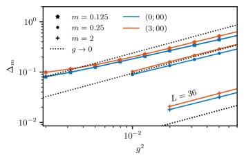
Figure 3: Weak coupling regime ($g^{2}\ll 1$) – Dependence of the gap on the coupling constant after subtracting the free case value $\Delta_{m}=(E-E_{0}-E_{\rm free})/m$ with $E_{\rm free}=2m,3m$ for mesons and baryons, respectively. We show the meson (empty purple) and baryon (filled gray) values for different masses. The dotted lines correspond to the weak coupling $(g^{2})^{2/3}$ expansion of Ziyatdinov (2010). The heavier mass is deep in the lattice regime and unsurprisingly shows large deviation. For smaller masses, the $\mathrm{QCD}_{2}$ is surprisingly close to the $\mathbb{Z}_{3}$ data. We further discuss the remaining finite volume effects in Fig.4. The $(g^{2})^{2/3}$ is a striking indication of confinement.

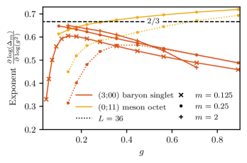
Figure 4: Leading exponent for small $g$ – Logarithmic derivative of data in Fig. 3. All the slopes converge to an exponent of $(g^{2})^{2/3}$. The bending of the curves away from the limiting value at small $g^{2}$ signal finite volume effects in this region. This is best appreciated by comparing the dotted circle with the plain circle; they correspond to data at the same mass but different volumes.

III.4 Topological edge modes vs. bulk excitations

Beyond the spectrum, we also study the spatial distribution of excited states. Because of staggering and open boundary conditions, the spatial structure of the ground state is non-trivial. Indeed, the use of staggered fermions in the Hamiltonian (7) gives it a simple topological nature with topologically protected edge modes at the open boundaries for the ground state. We emphasize, though, that this already also holds for the plain non-interacting model in the absence of any gauging, i.e., $g=0$, in which case the topological aspect is known as the Su-Schrieffer-Heeger (SSH) model Su et al. (1979); Batra and Sheet (2020). However, at finite $g$ this raises several non-trivial questions: (i) do the edge modes remain topologically protected when turning on finite $g$? (ii) if yes, how, are these edge modes characterized in terms of excess particle number and excess electric charge? (iii) to what extent is the nature of the excited states affected by the presence of open boundaries, i.e., are the excited states true bulk modes, or rather a property of the boundary?

The edge mode in the ground state for the non-interacting case ($g=0$) is analyzed in Fig. 5(a) at mass $m=0.2$ for an $L=60$ system. Clearly, the alternating onsite energy $\varepsilon_{x}=m(-1)^{x-1}$ directly translates to even/odd variations of the local occupations around the average filling $n_{0}=3/2$ (half-filling) throughout the system. However: this occupation pattern changes systematically towards the open boundaries. The data in Fig. 5(a) bends down at left boundary, and up at the right. The cumulative local particle number relative to half-filling, $N_{x}\equiv\sum_{x^{\prime}=1}^{x}(n_{x}-n_{0})$, is shown in Fig. 5(b), in light blue in the background. As this data is still alternating around a well-defind mean value, it is averaged over even and odd lengths [darker blue for $g=0$ in Fig. 5(b)]. This averaged data $\bar{N}_{x}$ shows that the particle number offset due to the open boundary is $n_{\rm edge}=\bar{N}_{x=L/2}=3/4$. The precise nature of the averaging matters here: by the procedure above, $\bar{N}_{x}=\sum_{x^{\prime}=1}^{x-1}(n_{x^{\prime}}-n_{0})+(n_{x}-n_{0})/2$. If instead, for example, one had computed the cumulative particle number over unit cells which pairs up neighboring sites, the resulting excess particle number would not have been strictly universal.

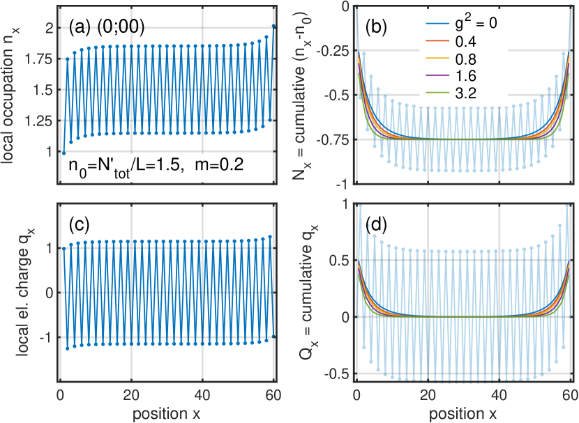
Figure 5: Edge modes for the QZD ground state, i.e., in the symmetry sector (0;00) for a system of size $L=60$ for $m=0.2$ – (a) Local particle number $n_{x}\equiv\langle\boldsymbol{\chi}_{x}^{\dagger}\cdot\boldsymbol{\chi}_{x}\rangle$ vs. position $i$ along the chain, for the free model $g^{2}=0$. Here $N^{\prime}_{\rm tot}\equiv\sum_{x}n_{x}$ is the actual, number of the filled Fermi sea given a finite lattice size. (b) Cumulative data in (a), after subtracting half-filling $n_{0}=N_{f}/2=3/2$ for each site, i.e., plotting $N_{x}\equiv\sum_{i^{\prime}=1}^{i}(n_{x}-n_{0})$. This data (light blue) still shows alternating behavior. Averaging over even and odd $x$ yields the smooth curve (solid darker blue). Additional averaged data for finite $g$ is presented in different colors, where the respective value of $g^{2}$ is specified in the legend. (c) Local electric charge based on Eq. (16). (d) (Averaged) cumulative data of (c) [similar analysis as in (b), also sharing the same legend].

Eventually, the cumulative excess particle number on the left boundary is exactly compensated at the right boundary. The cumulative total particle number offset over the entire system again returns to zero in Fig. 5(b). Therefore the excess particle number of the edge modes have the same value, but opposite signs for the two boundaries.

A non-zero interaction $g$ increases the gap in the system, see Fig. 2. Consistently, the edge modes localize more towards each open boundary (other colored lines in Fig. 5(b)). The topological aspect of the non-interacting model remains preserved as long as the gap does not close. Conversely, the topological protection remains intact in the presence of finite gauge strength $g$.

The value of the fractional excess particle number can be motivated straightforwardly for $g\to\infty$: there one has a simple product state of alternating completely empty and filled sites [see first line (ground state) in Fig. 1]. Therefore starting from the left open boundary, the particle number relative to half-filling is given by $n_{x}-n_{0}=[-n_{0},+n_{0},-n_{0},+n_{0},\ldots]$ with $n_{0}=3/2$. Its cumulative sum is $[-n_{0},0,-n_{0},0,\ldots]$. This averages to $-n_{0}/2$, and therefore $n_{\rm edge}=3/4$. This is precisely the excess number of particles observed in Fig. 5. For the extremal case here this excess particle number is strictly located right at the boundary. When reducing $g$, the edge mode starts to reach into the system as seen with Fig. 5(a). The cumulative excess particle number with each open boundary, nevertheless, remains pinned to precisely the same value

$$n_{\rm edge}=\frac{3}{4}=\frac{N_{f}}{4}\text{ .}$$ (24)

By having an odd number of flavors here, this shows that the edge mode carries a fractional particle number. This persists for any value of $g$ all the way down to $g=0$ since the gap of the system never closes. Hence as long as the system is long enough, such that the overlap of the tails of the boundary modes is negligible in the system center, one always obtains precisely the same value $\pm n_{\rm edge}$ for the excess particle number with opposite sign for the left and right boundary. Since this includes $g=0$, this shows that the topological protection of the SSH model remains intact also when gauging the system. Indeed, what protects SSH is inversion symmetry Wang et al. (2023). Gauging leaves this symmetry intact, e.g., for infinite systems or periodic systems of even length.

Now for a lattice gauge theory, by having an excess number of particles associated with an edge, one may worry that there is an electric field throughout the bulk connecting the two excess particle numbers of opposite sign for each boundary. However, this is not the case: while there is an excess number of particles due to the edge mode in the ground state, it does not carry any net effective electrical charge, therefore $q_{\rm edge}=0$.

This is demonstrated in the lower panels of Fig. 5 which repeats the same analysis as in the upper panels, but now for the electrical charge, using the number to charge conversion in Eq. (16). From the analysis in panel (d) one finds $q_{\rm edge}=\bar{Q}_{x=L/2}=0$. The smooth averaged curves in Fig. 5(b) simply got shifted to the zero base line in Fig. 5(d). This can be similarly motivated as for excess particle number above for the case $g\to\infty$: given the product state with alternating completely empty and filled sites, in the present case one obtains for the charge, starting from the left boundary, $q_{x}=[0,0,0,\ldots]$ which averages to zero, indeed.

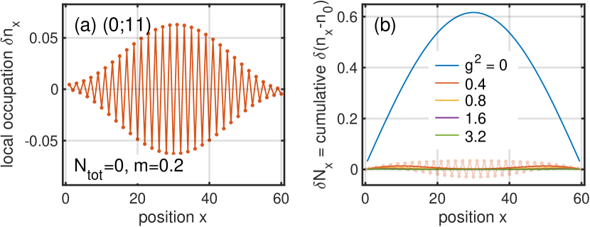
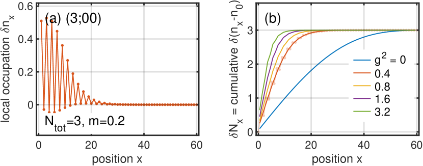
Figure 6: Lowest octet meson excitation [lowest energy eigenstate in the (0;11) symmetry sector] – (a) Difference of local particle number $\delta n_{x}$ relative to the ground state for $g^{2}=0.4$ [right legend also applies to panel (a); same parameters as in Fig. 5 otherwise]. (b) Cumulative data of (a) starting from the left boundary (light red) which is again even/odd averaged (solid red). Other smooth lines are obtained the same way for different $g^{2}$ as specified with the legend. Since this is a meson, eventually $\delta N_{\rm tot}=0$.

Figure 7: Lowest baryon excitation [lowest energy eigenstate in the (3;00) symmetry sector] – same analysis as in Fig. 7 otherwise. Since this is a baryon, eventually $\delta N_{\rm tot}=3$.

Having a clear understanding of the edge modes due to the open boundaries as discussed in Fig. 5, we now turn to excited states. Specifically, we want to ensure that low-energy baryon or meson excitations are true bulk excitations, and not a consequence of the presence of the open boundaries. In Fig. 7(a) we show the spatial distribution of the differential particle number occupation $\delta n_{x}$ for the octet meson $(0;11)$ relative to the ground state for $g^{2}=0.4$ (same parameters as in Fig. 5). The variations throughout the entire system clearly demonstrate the bulk nature of this excitation. The cumulative sum of the variation in Fig. 7(a) is shown in Fig. 7(b), supporting a similar picture. Since the total filling remained the same as for the ground state, the data in Fig. 7(b) returns to $\delta N=0$ for $x=L$. The variations in Fig. 7(b) diminish quickly, though, when increasing $g^{2}$ (smaller $g^{2}$ values will be analyzed in Fig. 8).

The lowest singlet baryon (b) excitation [(3;00) symmetry sector] is analyzed in Fig. 7. Analogous to the meson flavor excitation in Fig. 7, this again plots the differential variation of the particle number occupations $\delta n_{x}$ relative to the ground state. Figure 7(a) suggests that the baryon is (weakly) attracted to the left boundary. It is still a bulk excitation, though, in the sense that its extent clearly exceeds the penetration depth of the edge mode for the same $g^{2}=0.4$ as compared to Fig. 5(b).

By adding a baryon to the system, it is free to propagate. Via the kinetic term in the Hamiltonian (hopping term), the baryon has a tendency to delocalize across the entire system. Because of the gauge field, however, this motion generates electric fields which cost energy. Therefore in the presence of open boundaries, this energy is minimized by putting some of the excess particle number of $\Delta N_{\rm tot}=3$ right at the very first site of the left boundary as this site is particle-type: being below half-filled, this can hold more extra particles. Since there is no hopping to the left of the first site, there is less energy cost in terms of the electric field this would generate. This weak energetic bias towards the left boundary therefore is related to the convention that the system starts with particle-like site, i.e., with local energy $\varepsilon_{1}=m(-1)^{0}>0$. For this reason, we expect an isolated antibaryon ($\bar{b}$) to be attracted to the opposite boundary at the right. From this perspective, one may expect that the meson in Fig. 7(b) for sufficiently strong $g^{2}$ starts to split a $b\bar{b}$ pair separated to opposite boundaries. This is supported by the weak double peak structure that develops in Fig. 7(b) for larger $g^{2}$, indeed. Clear evidence for the same will be provided in Fig. 8.

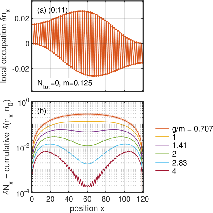
Figure 8: Same analysis as in Fig. 7, yet for the system parameters as in Fig. 2, i.e., for twice the system size $L=120$ here, while at the same time also smaller values of $g^{2}$ are used. Having $m=0.125$, the legend thus implies $g^{2}\leq(4m)^{2}=0.25$. The $x$-axis in (a) is the same as in (b), with (b) shown on semilog-y scale as compared to Fig. 7, in order to focus on the splitting of the data into a double peak structure.

It is instructive to track how excitations are distributed over a finite system with open boundaries as the interaction $g$ is increased. Let us start by discussing the baryon excitations. As one would expect from the continuum theory, the larger the coupling strength, the more localized the baryon state can become around a perturbation of an otherwise uniform system. In the present case this perturbation is given by the abrupt end of the system due to the open boundary. We expect such localization also to carry over to the lattice model. In the extremal case $g\to\infty$ where the ground state is a simple alternating product state as depicted at the top of Fig. 1, the baryon excitation simply fills any of the particle-like sites (last row in Fig. 1). This results in degeneracy, and thus a flat-band excitation. For large but finite $g$, there is a weak preference on the first site (left boundary) because of the earlier argument. This more apparently still here for large $g$, since the QZD interaction far dominates the kinetic energy. From the QZD perspective, due to the $\mathbb{Z}_{3}$ setup an excess charge of $\delta N_{x}=3$ does not generate an electric field since in that case the electric charge is effectively zero, $Q_{\rm tot}=0$. Hence for larger $g$, this confines the baryon in the neighborhood of the boundary as is seen in Fig. 7(b): the data quickly transitions from $\delta N_{x}=0\to 3$. Both, excess particle and electric charge are attracted to the left boundary. For $g\to 0$ eventually, the bias of the above type diminishes. At $g=0$ the baryon excitation is a true bulk excitation that is symmetric around the system center [blue line in Fig. 7(b)] up to even/odd alternations.

In this light we return to the low-energy mesons. We argued with the spectra in Fig. 2 that the meson singlet [in (0;00)] starts from a single particle/hole pair at weak coupling. For strong coupling, however, this becomes a $b\bar{b}$ pair. In Fig. 1 (third line) this is exemplified locally by shifting the particles from a completely filled site to a neighboring completely empty site.

From the present analysis we find that a single baryon is attracted to the left open boundary. By symmetry we argued that the antibaryon is attracted to the opposite boundary. Hence in the presence of $b\bar{b}$ meson at strong coupling, we expect due to the presence of the open boundaries, that the $b\bar{b}$ pair is dissocated towards the open boundaries as this permits a weak energy gain.

Revisiting Fig. 7(b), we find, indeed, that for larger $g^{2}$ a weak double peak structure develops in the data. In order to focus on this behavior, we repeat the analysis in Fig. 7(b) for the system parameters in Fig. 2 in Fig. 8 (hence twice the system length, yet also smaller $g$ values). By specifying $g$ in units of $m$ in the legend of Fig. 8(b), we find that the double peak structure develops around $g\simeq m$. At close inspection, the same also holds for the parameters in Fig. 7.

Hence the appearance and dissocation of the $b\bar{b}$ meson occurs far before the peak in the data towards large $g$ in Fig. 2: that peak in Fig. 2 is located around $g\sim 1/a$ where the coupling $g$ becomes stronger than the one-particle bandwidth. While the latter is a pure discretization effect, the dissocation of the $b\bar{b}$ occurs much sooner around $g\sim m$. Hence this behavior is expected to be a true property of QZD also in the continuum limit. The transition towards a $b\bar{b}$ meson around $g\sim m$ thus is consistent with the intuitiv notion that $g\sim m$ separates the weak from the strong coupling regime in the lattice gauge theory.

In the weak to intermediate coupling regime, the ground state (QZD vacuum) is far from the plain product state of alternating filled and empty sites as in Fig. 2, as seen for example, in Fig. 5(a). This way the QZD vacuum state acquires a non-trivial entanglement strucure. Similarly, the baryon, while attracted to the boundary, has significant spatial extent. As such, from a symmetry perspective, it can assume any flavor symmetry label that derives from the combination of three particles. In terms of ${\rm SU}(3)$ symmetry sectors this also permits octets $(11)$ aside the singlet $(00)$ and $(30)$ [cf. Eq. (32)]. Hence baryons (and also antibaryons) also exist in the octet representation $(11)$. In order to get an octet meson then, the simplest way to achieve this, is via an octet baryon with a singlet antibaryon or vice versa. Given that the octet meson splits $(b\bar{b})$ across the boundaries, the same may therefore also be expected for the simpler siuation of the meson singlet.

IV Summary and Outlook

In this work, we considered “QZD”, a $\mathbb{Z}_{3}$ gauge theory with three massive flavors of fermions in $1+1$ dimensions. We argued that thanks to the periodicity of Gauss’ law, it provides a unique opportunity to study “color” neutral isolated hadrons. Using state of the art tensor network simulations that take advantage of the full ${\rm U}(1)\times{\rm SU}(3)_{f}$ global symmetries, we determined the low-lying symmetry resolved spectrum of the theory for different masses. We identified two special points, where level crossing happens between the different symmetry sectors and that most probably correspond to special theories. We then confirmed that this system is in a confining phase by verifying a striking feature of confinement in $1+1$ dimensions: the small coupling expansion of hadrons is non analytic in $g^{2}$, and starts at order $(g^{2})^{2/3}$. We also studied the spatial distribution of the different excitations in our system. In particular, we confirmed that baryons are smaller at strong coupling. We also directly observed how the lightest meson transition from a single mesonic excitation to a pair of baryon-anti-baryon.

This work lays the ground for many potential exciting studies in $1+1$ dimensions and beyond. A very interesting feature of this model is that, thanks to the periodicity of Gauss law, the model can be studied with a non-zero baryon chemical potential, in the “color” neutral sector. Studying thermodynamical quantities as a function of $\mu$ appears as an interesting outlook. The system can also be put at finite temperature. Studying properties of “color neutral” baryons can be envisaged. Extending on our analysis of how excitations are distributed in space open the door to performing $1+1$ dimensional “tomography” of hadronic states. It could in particular inform on the size dependence of baryons as a function of coupling strength. In this direction, it appears that studying the model with two light flavors and one heavier one, reducing ${\rm SU}(3)_{f}$ to ${\rm SU}(2)_{f}\times{\rm U}(1)$ is of merit. Real-time dynamics and scattering processes can also be studied, in the ground state as well as at non-zero density. Extending the model to $2+1$ dimensions and studying its phase diagram is also an interesting avenue. Finally, this model presents itself as a natural contender for analog as well as digital quantum computations. In $1+1$ dimensions, it is of the same complexity as the Schwinger model but gives access to different physics. In higher-dimensions, the gauge fields do not need to be truncated and reduce the complexity burden associated to bosonic degrees of freedom.

Appendix A Weak coupling expansion

We derive here the weak coupling expansion (22) presented in the main text. The “Coulomb” potential is obtained by solving Gauss law for a test charge $E(x)=\frac{1}{2}\mathrm{Sign}(x)$ and integrating. To obtain the correct small coupling expansion, it is crucial to remember we are using staggered fermion, so that the correct non-relativistic potential is obtained by integrating up to $x/2$,

$$V(x)=\frac{g^{2}|x|}{4}\ .$$ (25)

(Equivalently, one could rescale $g^{2}\to g^{2}/2$ in Eq. 7.) The spectrum of the non-relativistic Hamiltonian is found by solving the associated non-relativistic Schrödinger equation Fonseca and Zamolodchikov (2006); Fateev et al. (2009); Ziyatdinov (2010); Zubov et al. (2015). As suggested by dimensional analysis, after rescaling $x\to y/(mg^{2})^{1/3}$,

$$\left(\frac{g^{4}}{m}\right)^{1/3}\left(-\frac{1}{2}\frac{d^{2}}{dy^{2}}+\frac{|y|}{4}\right)\psi(y)=E_{n}\psi(y)\,.$$ (26)

The function $\psi(y)$ are solutions to the Airy equations. Imposing continuity relations, we get

$$\psi(y)\sim\mathrm{Ai}\left(\left(\frac{4m}{g^{4}}\right)^{1/3}\left(-2E_{n}+\frac{1}{2}g^{2}y\right)\right)\,.$$ (27)

Valid solutions are split into symmetric and antisymmetric sectors. The symmetric sector is characterized by $\psi^{\prime}(0)=0$ and contains the lowest-lying meson. The first zero of $\mathrm{Ai}^{\prime}(-z)$ is $z\approx 1.01879$ DLMF , which gives Eq. (22).

This analysis is identical to that in the ’t Hooft model ’t Hooft (1974); Fonseca and Zamolodchikov (2006); Fateev et al. (2009); Ziyatdinov (2010); Zubov et al. (2015), which is a ${\rm SU}(N)$ gauge theory in $1+1$ dimensions as $N\rightarrow\infty$, keeping the number of quark flavors, $N_{f}$ fixed. In this limit corrections to the gluon propagator from the quark loop are suppressed by $\sim N_{f}/N_{c}$, and the gluon propagator remains $=1/k^{2}$ for any value of the coupling constant. In contrast, for QED in $1+1$ dimensions, in general the photon propagator is modified by fermion loops. However, in weak coupling, where $g^{2}/m^{2}\rightarrow 0$, corrections to the photon propagator from fermion loops are suppressed by $\sim(g^{2}/m^{2})^{1/3}$, and so can be neglected.

Appendix B Symmetry labels

The Hamiltonian in Eq. (7) preserves particle number and is fully symmetric in its $N_{f}=3$ fermionic flavors. Hence it has ${\rm U}(1)_{\rm N}\otimes{\rm SU}(3)_{\rm flavor}$ symmetry. We fully exploit these symmetries in our numerical simulations by utilizing the QSpace tensor library Weichselbaum (2012b, 2020, 2006-2023). Accordingly, we can differentiate all eigenstates according to these symmetry sectors.

We specify symmetry labels in terms of the tuple of three integer values

$$q \equiv (q_{0};q_{1},q_{2})\equiv(q_{0};q_{1}q_{2})$$ (28)

where $q_{0}\in\mathbb{Z}$ specifies the total number of particles relative to half-filling, and $(q_{1},q_{2})\equiv(q_{1}q_{2})$ specifies the ${\rm SU}(3)$ multiplet. The latter are based on the standard multiplet labels for ${\rm SU}(N)$ that directly specify the respective Young tableaux Young (1930); Cahn (1984). This requires two labels $q_{1},q_{2}\geq 0$ for an ${\rm SU}(3)$ multiplet which specify a Young tableaux of two rows,

(29)

where $q_{1}$ and $q_{2}$ indicate the offset of extra boxes per row, starting from the top. This concept generalizes to general ${\rm SU}(N)$ Cahn (1984) with $N-1$ rows there. E.g, for ${\rm SU}(2)$, $q_{1}=2S$. Completely filled columns of $N$ boxes represent singlets and can be skipped from the tableau.

Local state space

With the symmetries above, all $2^{3}=8$ states of a single site are organized into symmetry multiplets as follows: the completely filled state has symmetry labels $(3/2;00)$, the completely empty state $(-3/2;00)$. Half-integer particle numbers here is simply due the definition of subtracting half-filling $n_{0}=3/2$, and has no further relevance otherwise The same also holds for blocks containing an odd number of sites. The three states with only one particle transform in the defining representation of ${\rm SU}(3)$, hence represent the combined symmetry multiplet $(-1/2;10)$. Conversely, removing a particle from the completely filled state transforms in the dual to the defining representation. Hence these states represent the symmetry multiplet $(1/2;01)$. In their union, $1+1+3+3=8$, this exhausts the local state space.

We note that having half-integers for particle number is purely due to the definition ‘relative to half-filling’. In practice, via the tensor library QSpace Weichselbaum (2012b) we use twice the particle number relative to half-filling, such that the symmetry label for the local particle number of a site relative to half-filling is also an integer, having $2n^{\prime}\in\{-3,-1,1,3\}$ for a single site.

Examples for ${\rm SU}(3)$

The defining representation has symmetry labels $(10)\equiv{\bf 3}$, and its dual $(01)\equiv\bar{\bf 3}$. The ‘spin’ operator transforms in the adjoint representation $(11)\equiv{\bf 8}$ (octet),

$${\bf 3}\otimes\bar{\bf 3}\equiv(10)\otimes(01)=(00)+(11)\text{ ,}$$ (30)

with $(00)\equiv{\bf 1}$ the scalar representation (singlet). This also represents the symmetry labels of a single particle-hole excitation (cf. meson). Note that this is completely analogous to ${\rm SU}(2)$ where $\frac{1}{2}\otimes\frac{1}{2}=0+1$, with $S=1$ the ${\rm SU}(2)$ spin operator.

Two particles transform in the combined space

$${\bf 3}\otimes{\bf 3}\equiv(10)\otimes(10)=(20)+(01)\text{ ,}$$ (31)

with $(20)\equiv{\bf 6}$ the symmetric, and $(01)\equiv\bar{\bf 3}$ the antisymmetric subspace. Three particles like the baryon transform in the combined space

$${\bf 3}\otimes{\bf 3}\otimes{\bf 3} \equiv (10)\otimes(10)\otimes(10)$$ (32)

$$= (00)+(11)^{2}+(30)\text{ ,}$$

where superscript indicates multiplicities, and $(30)\equiv{\bf 10}$ is a fully symmetric multiplet. Dual representations are simply given by $q=(q_{1}q_{2})\to\bar{q}=(q_{2},q_{1})$. Hence all ireps with $q_{1}=q_{2}$ are self-dual, while all others are not.

We emphasize that the specification of an irreducible representation (irep) for ${\rm SU}(N>2)$ via the single label of its multiplet dimension only is generally insufficient because it is not unique. For example for ${\rm SU}(3)$, the ireps (40) and (21) accidentally share the same multiplet dimension $d=15$ together with their respective duals (04) and (12).

Appendix C DMRG convergence

We use DMRG White (1992); Schollwöck (2011) in the fermionic setting where we fully exploit the ${\rm SU}(3)$ flavor symmetry for the sake of numerical efficiency Weichselbaum (2012b, 2020, 2006-2023). Data such as in Fig. 2 was obtained by simultaneously targeting several low energy multiplets (cf. App. B): this included 4 multiplets in $(0,00)$, and one multiplet in each of $(\pm 3,00)$, $(0,11)$, and $(3,11)$, i.e., a total of $8$ multiplets, or equivalently, $6+2\times 8=20$ states.

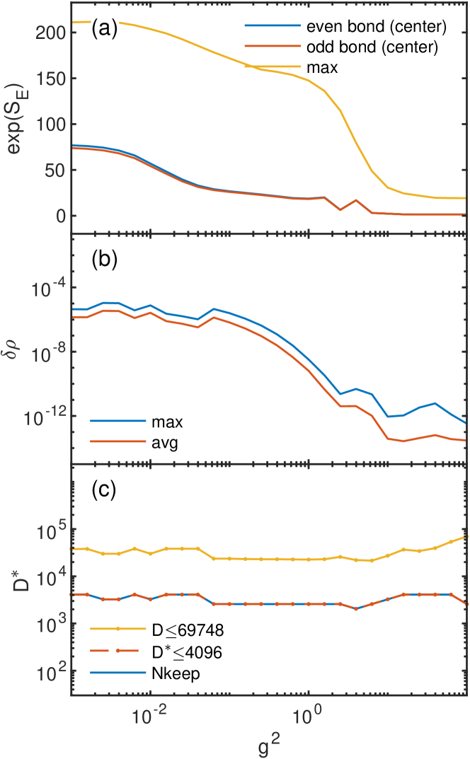
Figure 9: DMRG convergence analysis for the data in Fig. 2 vs. QZ3 coupling $g^{2}$ (having $m=0.125$, $L=120$). In the simulations a total of 8 multiplets was targeted simultaneously: 4 multiplets in $(0,00)$, and one multiplet in each of $(\pm 3,00)$, $(0,11)$, and $(3,11)$, corresponding to a total of $6+2\times 8=20$ states. (a) Exponentiated block entanglement entropy in the system center, and also the overall maximum along chain (the entanglement profile is strongly asymmetric around the system center, because multiple states are targeted). (b) Maximum and average discarded weight for last 2-site DMRG sweep. (c) DMRG bond dimension in last sweep, keeping up to $N_{\rm keep}=D^{\ast}\leq 4,096$ multiplets (corresponding up to $D\leq 69,748$ states).

The bond dimension in terms of $D^{\ast}$ multiplets was usually ramped up uniformly in an exponential way, increasing it by a factor of $2^{1/3}\sim 1.26$ for each full sweep. By keeping up to $D^{\ast}=4,096$ multiplets, this effectively corresponded to keeping up to $D\sim 70,000$ states [Fig. 9(c)]. Thus by fully exploiting ${\rm SU}(3)$ flavor symmetry, the effective bond dimension was effectively reduced by an average factor of $\sim 17$ by switching to a multiplet-based description. Bearing in mind, that the numerical cost of DMRG scales like $\mathcal{O}(D^{3})$, this implies a gain in numerical efficiency by at least three orders of magnitude.

For the data in Fig. 2, overall, this gave rise to a discarded weight of $\delta\rho\lesssim 10^{-5}$ as shown in Fig. 9, with the entanglement entropy [Fig. 9(a)] and thus also the discarded weight largest for small $g$.

Appendix D Mapping to spin Hamiltonian

In this appendix, we provide the spin-chain equivalent of Eq. (7). We obtain in using a standard Jordan-Wigner transformation and provide it only to assist the interested reader.

We introduce $3\cdot N$ spin operators $\sigma^{x,y,z}_{I},\sigma^{\pm}_{I}=1/2(\sigma_{I}^{x}\pm\sigma_{I}^{y})$, labeling them with an index $I=(n-1)\cdot 3+f$ which uniquely maps onto indices $(n,f)$ for the position in the lattice, $n$ and the flavor, $f$. The Jordan-Wigner transformation becomes $\chi_{I}=\sigma^{-}_{I}\prod_{J=1}^{I-1}\sigma^{z}_{J}$, and generates the spin Hamiltonian

$$H=\sum_{n=1}^{N}\sum_{f=1}^{3}\left(-\frac{i}{2a}\sigma^{+}_{n,f}\sigma^{-}_{n+1,f}S^{n+1,f}_{n,f}+\mathrm{h.c.}\right)$$

$$+\sum_{x=n}^{N}\sum_{f=1}^{3}\left(\frac{m}{2}(-1)^{n}\sigma^{z}_{n,f}\right)$$ (33)

$$+\frac{g^{2}}{2}\sum_{n=1}^{N}\left(\frac{2\pi}{3}\sum_{l=1}^{n}\left(\left(\frac{\sigma^{z}_{n,f}}{2}+\frac{(-1)^{n}}{2}\right)\,\textrm{mod}\,3\right)\right)^{2},$$

where $S^{n+1,f}_{n,f}=\prod_{J=3n-3+f}^{3n+f}\sigma^{z}_{J}$ is a string of $\sigma^{z}_{n,f}$ operators arising from the multi-flavor Jordan-Wigner transform. Similar strings arise in mapping a ${\rm SU}(3)$ gauge theory in $1+1$ dimensions onto spin variables Farrell et al. (2023).

Appendix E Nonzero chemical potential

We present in this appendix exploratory results of QZD at non-zero baryon chemical potential. They are of value for this work as they provide a completely independent determination of the baryon mass and provide a convincing cross-check of our numerical analysis. For context,the behavior of QCD at low temperatures and chemical potential is directly relevant to the collision of heavy ions at moderate energies Kumar et al. (2023) and to the behavior of neutron stars as observed by multimessenger astronomy Dietrich et al. (2020). At non-zero quark chemical potential $\mu_{\rm qk}$ the quark determinant in the Euclidean action is complex, and so direct numerical simulations using importance sampling are not possible. When $\mu_{\rm qk}<T$, thermodynamics quantities can be computed in several ways, including: expanding in a Taylor series in $\mu_{\rm qk}$ Borsanyi et al. (2020); Bollweg et al. (2022, 2023); Mitra et al. (2022); Mitra and Hegde (2023); analytic continuation from imaginary chemical potential Ishii et al. (2019); Begun et al. (2021); Bornyakov et al. (2023); Brandt et al. (2022); reweighting techniques Borsanyi et al. (2022, 2023); strong coupling expansions Gagliardi and Unger (2020); Philipsen and Scheunert (2019); Kim et al. (2020); Klegrewe and Unger (2020); Philipsen (2021a, b); Kim et al. (2023); complex Langevin equations Kogut and Sinclair (2019); Sexty (2019); Ito et al. (2020); Seiler et al. (2023); approximate solutions of the Schwinger-Dyson equations Isserstedt et al. (2019); Gunkel and Fischer (2021); Bernhardt et al. (2021); and the functional renormalization group Gao and Pawlowski (2020); Dupuis et al. (2021); Isserstedt et al. (2021); Fu et al. (2021); Chen et al. (2021); Ayala et al. (2022); Fu (2022); Otto et al. (2022); Fu et al. (2023); Bernhardt and Fischer (2023).

As a first step we consider QZD at $\mu\neq 0$, finding the ground state of

$$H_{\mu}=H_{0}-\mu\sum_{x}n_{x}\ ,$$ (34)

as a function of $\mu$, with $H_{0}$ the Hamiltonian in Eq. (1). For this simulation we had used the package ITensor Fishman et al. (2022a, b) without imposing any symmetry constraint. In this DMRG simulation we kept up to $600$ states.

In Fig. 10 we show the expectation value of the particle number as a function of $\mu$. It vanishes until $\mu=m_{(3,00)}$, where $m_{(3,00)}$ is the mass of the lightest baryon. It is then constant until it jumps again, to various multiples of three. That the number density vanishes until $\mu>m_{(3,00)}$ illustrates ”silver blaze” phenomenon Cohen (2004); Aarts (2016): the ground state at $\mu=0$ remains the ground state of the grand canonical ensemble until the chemical potential exceeds the mass of the lightest state which carries fermion number It is an important consistency check that $m_{(3,00)}$ determined from the silver blaze phenomenon agrees with the direct calculation in Sec. III.3. That the number density only jumps to multiples of three follows from gauge invariance under the local $\mathbb{Z}_{3}$ symmetry: baryons always carry $u$, $d$, and $s$ fermions in common multiples. This is in contrast to a ${\rm U}(1)$ gauge theory, where as we showed in the Sec. I, Gauss’s law excludes a nonzero value for the electric charge, or fermion number. As $L\rightarrow\infty$, Fig. 10 would be a smooth curve, with $N/L$ a smoothly varying function. For finite $L$, however, this is a series of steps that increases in multiples of three, thus guaranteeing a well-defined baryon number. The absence of some multiples of three is an artifact due to our resolution in $\mu$. Note also that the fact the first plateau is larger than the other can probably be attributed to the open boundary as discussed with Fig. 7 in the main text.

A more detailed study at finite chemical potential is left for future work.

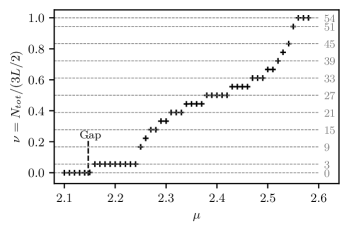
Figure 10: The total number of particles as a function of the chemical potential, for $m=2$, $L=36$ and $g^{2}=1.466$. The vertical axis is scaled such that $\nu=1$ is a completely filled system.

References

- Wilson (1974) Kenneth G. Wilson, “Confinement of Quarks,” Phys. Rev. D 10, 2445–2459 (1974).
- Kogut and Susskind (1974) John B. Kogut and Leonard Susskind, “Vacuum Polarization and the Absence of Free Quarks in Four-Dimensions,” Phys. Rev. D 9, 3501–3512 (1974).
- Fradkin (2013) Eduardo H. Fradkin, Field Theories of Condensed Matter Physics, Vol. 82 (Cambridge Univ. Press, Cambridge, UK, 2013).
- Schwinger (1962) Julian S. Schwinger, “Gauge Invariance and Mass. 2.” Phys. Rev. 128, 2425–2429 (1962).
- Banks et al. (1976) Tom Banks, Leonard Susskind, and John B. Kogut, “Strong Coupling Calculations of Lattice Gauge Theories: (1+1)-Dimensional Exercises,” Phys. Rev. D 13, 1043 (1976).
- Coleman et al. (1975) Sidney R. Coleman, R. Jackiw, and Leonard Susskind, “Charge Shielding and Quark Confinement in the Massive Schwinger Model,” Annals Phys. 93, 267 (1975).
- Coleman (1976) Sidney R. Coleman, “More About the Massive Schwinger Model,” Annals Phys. 101, 239 (1976).
- Manton (1985) N. S. Manton, “The Schwinger Model and Its Axial Anomaly,” Annals Phys. 159, 220–251 (1985).
- ’t Hooft (1974) Gerard ’t Hooft, “A Two-Dimensional Model for Mesons,” Nucl. Phys. B 75, 461–470 (1974).
- Callan et al. (1976) Curtis G. Callan, Jr., Nigel Coote, and David J. Gross, “Two-Dimensional Yang-Mills Theory: A Model of Quark Confinement,” Phys. Rev. D 13, 1649 (1976).
- Fonseca and Zamolodchikov (2006) Pedro Fonseca and Alexander Zamolodchikov, “Ising spectroscopy. I. Mesons at T T(c),” (2006), arXiv:hep-th/0612304 .
- Fateev et al. (2009) V. A. Fateev, S. L. Lukyanov, and A. B. Zamolodchikov, “On mass spectrum in ’t Hooft’s 2D model of mesons,” J. Phys. A 42, 304012 (2009), arXiv:0905.2280 [hep-th] .
- Ziyatdinov (2010) Iskander Ziyatdinov, “Asymptotic properties of mass spectrum in ’t Hooft’s model of mesons,” Int. J. Mod. Phys. A 25, 3899–3910 (2010), arXiv:1003.4304 [hep-th] .
- Zubov et al. (2015) R. A. Zubov, S. A. Paston, and E. V. Prokhvatilov, “Exact solution of the ’t Hooft equation in the limit of heavy quarks with unequal masses,” Theor. Math. Phys. 184, 1281–1286 (2015).
- Buyens et al. (2014) Boye Buyens, Jutho Haegeman, Karel Van Acoleyen, Henri Verschelde, and Frank Verstraete, “Matrix product states for gauge field theories,” Phys. Rev. Lett. 113, 091601 (2014), arXiv:1312.6654 [hep-lat] .
- Bañuls et al. (2013) M. C. Bañuls, K. Cichy, K. Jansen, and J. I. Cirac, “The mass spectrum of the Schwinger model with Matrix Product States,” JHEP 11, 158 (2013), arXiv:1305.3765 [hep-lat] .
- Cirac et al. (2021) J. Ignacio Cirac, David Perez-Garcia, Norbert Schuch, and Frank Verstraete, “Matrix product states and projected entangled pair states: Concepts, symmetries, theorems,” Rev. Mod. Phys. 93, 045003 (2021), arXiv:2011.12127 [quant-ph] .
- Hauke et al. (2013) Philipp Hauke, David Marcos, Marcello Dalmonte, and Peter Zoller, “Quantum simulation of a lattice Schwinger model in a chain of trapped ions,” Phys. Rev. X 3, 041018 (2013), arXiv:1306.2162 [cond-mat.quant-gas] .
- Rico et al. (2014) E. Rico, T. Pichler, M. Dalmonte, P. Zoller, and S. Montangero, “Tensor networks for Lattice Gauge Theories and Atomic Quantum Simulation,” Phys. Rev. Lett. 112, 201601 (2014), arXiv:1312.3127 [cond-mat.quant-gas] .
- Pichler et al. (2016) T. Pichler, M. Dalmonte, E. Rico, P. Zoller, and S. Montangero, “Real-time Dynamics in U(1) Lattice Gauge Theories with Tensor Networks,” Phys. Rev. X 6, 011023 (2016), arXiv:1505.04440 [cond-mat.quant-gas] .
- Zohar et al. (2016) Erez Zohar, J. Ignacio Cirac, and Benni Reznik, “Quantum Simulations of Lattice Gauge Theories using Ultracold Atoms in Optical Lattices,” Rept. Prog. Phys. 79, 014401 (2016), arXiv:1503.02312 [quant-ph] .
- Martinez et al. (2016) E. A. Martinez et al., “Real-time dynamics of lattice gauge theories with a few-qubit quantum computer,” Nature 534, 516–519 (2016), arXiv:1605.04570 [quant-ph] .
- Muschik et al. (2017) Christine Muschik, Markus Heyl, Esteban Martinez, Thomas Monz, Philipp Schindler, Berit Vogell, Marcello Dalmonte, Philipp Hauke, Rainer Blatt, and Peter Zoller, “U(1) Wilson lattice gauge theories in digital quantum simulators,” New J. Phys. 19, 103020 (2017), arXiv:1612.08653 [quant-ph] .
- Klco et al. (2018) N. Klco, E. F. Dumitrescu, A. J. McCaskey, T. D. Morris, R. C. Pooser, M. Sanz, E. Solano, P. Lougovski, and M. J. Savage, “Quantum-classical computation of Schwinger model dynamics using quantum computers,” Phys. Rev. A 98, 032331 (2018), arXiv:1803.03326 [quant-ph] .
- Bañuls et al. (2020) M. C. Bañuls et al., “Simulating Lattice Gauge Theories within Quantum Technologies,” Eur. Phys. J. D 74, 165 (2020), arXiv:1911.00003 [quant-ph] .
- Surace et al. (2020) Federica M. Surace, Paolo P. Mazza, Giuliano Giudici, Alessio Lerose, Andrea Gambassi, and Marcello Dalmonte, “Lattice gauge theories and string dynamics in Rydberg atom quantum simulators,” Phys. Rev. X 10, 021041 (2020), arXiv:1902.09551 [cond-mat.quant-gas] .
- Bañuls and Cichy (2020) Mari Carmen Bañuls and Krzysztof Cichy, “Review on Novel Methods for Lattice Gauge Theories,” Rept. Prog. Phys. 83, 024401 (2020), arXiv:1910.00257 [hep-lat] .
- Yang et al. (2020) Bing Yang, Hui Sun, Robert Ott, Han-Yi Wang, Torsten V. Zache, Jad C. Halimeh, Zhen-Sheng Yuan, Philipp Hauke, and Jian-Wei Pan, “Observation of gauge invariance in a 71-site Bose–Hubbard quantum simulator,” Nature 587, 392–396 (2020), arXiv:2003.08945 [cond-mat.quant-gas] .
- Rigobello et al. (2021) Marco Rigobello, Simone Notarnicola, Giuseppe Magnifico, and Simone Montangero, “Entanglement generation in (1+1)D QED scattering processes,” Phys. Rev. D 104, 114501 (2021), arXiv:2105.03445 [hep-lat] .
- Rigobello et al. (2023) Marco Rigobello, Giuseppe Magnifico, Pietro Silvi, and Simone Montangero, “Hadrons in (1+1)D Hamiltonian hardcore lattice QCD,” (2023), arXiv:2308.04488 [hep-lat] .
- Desaules et al. (2023) Jean-Yves Desaules, Debasish Banerjee, Ana Hudomal, Zlatko Papić, Arnab Sen, and Jad C. Halimeh, “Weak ergodicity breaking in the Schwinger model,” Phys. Rev. B 107, L201105 (2023), arXiv:2203.08830 [cond-mat.str-el] .
- Chanda et al. (2020) Titas Chanda, Jakub Zakrzewski, Maciej Lewenstein, and Luca Tagliacozzo, “Confinement and lack of thermalization after quenches in the bosonic Schwinger model,” Phys. Rev. Lett. 124, 180602 (2020), arXiv:1909.12657 [cond-mat.stat-mech] .
- Kühn et al. (2015) Stefan Kühn, Erez Zohar, J. Ignacio Cirac, and Mari Carmen Bañuls, “Non-Abelian string breaking phenomena with Matrix Product States,” JHEP 07, 130 (2015), arXiv:1505.04441 [hep-lat] .
- Magnifico et al. (2020) Giuseppe Magnifico, Marcello Dalmonte, Paolo Facchi, Saverio Pascazio, Francesco V. Pepe, and Elisa Ercolessi, “Real Time Dynamics and Confinement in the Schwinger-Weyl lattice model for 1+1 QED,” Quantum 4, 281 (2020), arXiv:1909.04821 [quant-ph] .
- de Jong et al. (2022) Wibe A. de Jong, Kyle Lee, James Mulligan, Mateusz Płoskoń, Felix Ringer, and Xiaojun Yao, “Quantum simulation of nonequilibrium dynamics and thermalization in the Schwinger model,” Phys. Rev. D 106, 054508 (2022), arXiv:2106.08394 [quant-ph] .
- Lee et al. (2023) Kyle Lee, James Mulligan, Felix Ringer, and Xiaojun Yao, “Liouvillian Dynamics of the Open Schwinger Model: String Breaking and Kinetic Dissipation in a Thermal Medium,” (2023), arXiv:2308.03878 [quant-ph] .
- Florio et al. (2023) Adrien Florio, David Frenklakh, Kazuki Ikeda, Dmitri Kharzeev, Vladimir Korepin, Shuzhe Shi, and Kwangmin Yu, “Real-Time Nonperturbative Dynamics of Jet Production in Schwinger Model: Quantum Entanglement and Vacuum Modification,” Phys. Rev. Lett. 131, 021902 (2023), arXiv:2301.11991 [hep-ph] .
- Zache et al. (2019) T. V. Zache, N. Mueller, J. T. Schneider, F. Jendrzejewski, J. Berges, and P. Hauke, “Dynamical Topological Transitions in the Massive Schwinger Model with a Term,” Phys. Rev. Lett. 122, 050403 (2019), arXiv:1808.07885 [quant-ph] .
- Kharzeev and Kikuchi (2020) Dmitri E. Kharzeev and Yuta Kikuchi, “Real-time chiral dynamics from a digital quantum simulation,” Phys. Rev. Res. 2, 023342 (2020), arXiv:2001.00698 [hep-ph] .
- Ikeda et al. (2021) Kazuki Ikeda, Dmitri E. Kharzeev, and Yuta Kikuchi, “Real-time dynamics of Chern-Simons fluctuations near a critical point,” Phys. Rev. D 103, L071502 (2021), arXiv:2012.02926 [hep-ph] .
- Witten (1979) Edward Witten, “Baryons in the 1/n Expansion,” Nucl. Phys. B 160, 57–115 (1979).
- Steinhardt (1980) Paul J. Steinhardt, “Baryons and Baryonium in QCD in Two-dimensions,” Nucl. Phys. B 176, 100–112 (1980).
- Bringoltz (2009) Barak Bringoltz, “Solving two-dimensional large-N QCD with a nonzero density of baryons and arbitrary quark mass,” Phys. Rev. D 79, 125006 (2009), arXiv:0901.4035 [hep-lat] .
- Lajer et al. (2022) Marton Lajer, Robert M. Konik, Robert D. Pisarski, and Alexei M. Tsvelik, “When cold, dense quarks in 1+1 and 3+1 dimensions are not a Fermi liquid,” Phys. Rev. D 105, 054035 (2022), arXiv:2112.10238 [hep-th] .
- Rico et al. (2018) E. Rico, M. Dalmonte, P. Zoller, D. Banerjee, M. Bögli, P. Stebler, and U. J. Wiese, “SO(3) ”Nuclear Physics” with ultracold Gases,” Annals Phys. 393, 466–483 (2018), arXiv:1802.00022 [cond-mat.quant-gas] .
- Farrell et al. (2023) Roland C. Farrell, Ivan A. Chernyshev, Sarah J. M. Powell, Nikita A. Zemlevskiy, Marc Illa, and Martin J. Savage, “Preparations for quantum simulations of quantum chromodynamics in 1+1 dimensions. I. Axial gauge,” Phys. Rev. D 107, 054512 (2023), arXiv:2207.01731 [quant-ph] .
- Gervais and Sakita (1978) Jean-Loup Gervais and B. Sakita, “Gauge degrees of freedom, external charges, quark confinement criterion in = 0 canonical formalism,” Phys. Rev. D 18, 453 (1978).
- Pisarski (2022) Robert D. Pisarski, “Wilson loops in the Hamiltonian formalism,” Phys. Rev. D 105, L111501 (2022), arXiv:2202.11122 [hep-th] .
- Kaplan et al. (2023) David E. Kaplan, Tom Melia, and Surjeet Rajendran, “The Classical Equations of Motion of Quantized Gauge Theories, Part 2: Electromagnetism,” (2023), arXiv:2307.09475 [hep-th] .
- Dumitru et al. (2005) Adrian Dumitru, Robert D. Pisarski, and Detlef Zschiesche, “Dense quarks, and the fermion sign problem, in a SU(N) matrix model,” Phys. Rev. D 72, 065008 (2005), arXiv:hep-ph/0505256 .
- Narayanan (2012) R. Narayanan, “Two flavor massless Schwinger model on a torus at a finite chemical potential,” Phys. Rev. D 86, 125008 (2012), arXiv:1210.3072 [hep-th] .
- Lohmayer and Narayanan (2013) Robert Lohmayer and Rajamani Narayanan, “Phase structure of two-dimensional QED at zero temperature with flavor-dependent chemical potentials and the role of multidimensional theta functions,” Phys. Rev. D 88, 105030 (2013), arXiv:1307.4969 [hep-th] .
- Bañuls et al. (2017) Mari Carmen Bañuls, Krzysztof Cichy, J. Ignacio Cirac, Karl Jansen, and Stefan Kühn, “Density Induced Phase Transitions in the Schwinger Model: A Study with Matrix Product States,” Phys. Rev. Lett. 118, 071601 (2017), arXiv:1611.00705 [hep-lat] .
- Pisarski (2021) Robert D. Pisarski, “Remarks on nuclear matter: How an condensate can spike the speed of sound, and a model of baryons,” Phys. Rev. D 103, L071504 (2021), arXiv:2101.05813 [nucl-th] .
- Weichselbaum (2012a) Andreas Weichselbaum, “Non-abelian symmetries in tensor networks: A quantum symmetry space approach,” Annals of Physics 327, 2972–3047 (2012a).
- Orus (2014) Roman Orus, “A Practical Introduction to Tensor Networks: Matrix Product States and Projected Entangled Pair States,” Annals Phys. 349, 117–158 (2014), arXiv:1306.2164 [cond-mat.str-el] .
- Fishman et al. (2020) Matthew Fishman, Steven R. White, and E. Miles Stoudenmire, “The ITensor Software Library for Tensor Network Calculations,” (2020), 10.21468/SciPostPhysCodeb.4, arXiv:2007.14822 [cs.MS] .
- Meurice et al. (2022) Yannick Meurice, Ryo Sakai, and Judah Unmuth-Yockey, “Tensor lattice field theory for renormalization and quantum computing,” Rev. Mod. Phys. 94, 025005 (2022), arXiv:2010.06539 [hep-lat] .
- Greensite (2017) Jeff Greensite, “Confinement from Center Vortices: A review of old and new results,” EPJ Web Conf. 137, 01009 (2017), arXiv:1610.06221 [hep-lat] .
- Sale et al. (2023) Nicholas Sale, Biagio Lucini, and Jeffrey Giansiracusa, “Probing center vortices and deconfinement in SU(2) lattice gauge theory with persistent homology,” Phys. Rev. D 107, 034501 (2023), arXiv:2207.13392 [hep-lat] .
- Biddle et al. (2022a) James C. Biddle, Waseem Kamleh, and Derek B. Leinweber, “Static quark potential from center vortices in the presence of dynamical fermions,” Phys. Rev. D 106, 054505 (2022a), arXiv:2206.00844 [hep-lat] .
- Biddle et al. (2022b) James C. Biddle, Waseem Kamleh, and Derek B. Leinweber, “Impact of dynamical fermions on the center vortex gluon propagator,” Phys. Rev. D 106, 014506 (2022b), arXiv:2206.02320 [hep-lat] .
- Biddle et al. (2023) James C. Biddle, Waseem Kamleh, and Derek B. Leinweber, “Center vortex structure in the presence of dynamical fermions,” Phys. Rev. D 107, 094507 (2023), arXiv:2302.05897 [hep-lat] .
- Horn et al. (1979) D. Horn, M. Weinstein, and S. Yankielowicz, “HAMILTONIAN APPROACH TO Z(N) LATTICE GAUGE THEORIES,” Phys. Rev. D 19, 3715 (1979).
- Kogut et al. (1980) J. B. Kogut, R. B. Pearson, J. Shigemitsu, and D. K. Sinclair, “() and State Potts Lattice Gauge Theories: Phase Diagrams, First Order Transitions, Beta Functions and Expansions,” Phys. Rev. D 22, 2447 (1980).
- Kogut (1980) John B. Kogut, “1/n Expansions and the Phase Diagram of Discrete Lattice Gauge Theories With Matter Fields,” Phys. Rev. D 21, 2316 (1980).
- Alcaraz and Koberle (1981) F. C. Alcaraz and R. Koberle, “The Phases of Two-dimensional Spin and Four-dimensional Gauge Systems With Symmetry,” J. Phys. A 14, 1169 (1981).
- Alcaraz and Koberle (1980) F. C. Alcaraz and R. Koberle, “Duality and the Phases of (n) Spin Systems,” J. Phys. A 13, L153 (1980).
- Zohar et al. (2017) Erez Zohar, Alessandro Farace, Benni Reznik, and J. Ignacio Cirac, “Digital lattice gauge theories,” Phys. Rev. A 95, 023604 (2017), arXiv:1607.08121 [quant-ph] .
- Ercolessi et al. (2018) Elisa Ercolessi, Paolo Facchi, Giuseppe Magnifico, Saverio Pascazio, and Francesco V. Pepe, “Phase Transitions in Gauge Models: Towards Quantum Simulations of the Schwinger-Weyl QED,” Phys. Rev. D 98, 074503 (2018), arXiv:1705.11047 [quant-ph] .
- Magnifico et al. (2019a) G. Magnifico, D. Vodola, E. Ercolessi, S. P. Kumar, M. Müller, and A. Bermudez, “Symmetry-protected topological phases in lattice gauge theories: topological QED2,” Phys. Rev. D 99, 014503 (2019a), arXiv:1804.10568 [cond-mat.quant-gas] .
- Magnifico et al. (2019b) G. Magnifico, D. Vodola, E. Ercolessi, S. P. Kumar, M. Müller, and A. Bermudez, “ gauge theories coupled to topological fermions: QED2 with a quantum-mechanical angle,” Phys. Rev. B 100, 115152 (2019b), arXiv:1906.07005 [cond-mat.quant-gas] .
- Borla et al. (2020) Umberto Borla, Ruben Verresen, Fabian Grusdt, and Sergej Moroz, “Confined Phases of One-Dimensional Spinless Fermions Coupled to Gauge Theory,” Phys. Rev. Lett. 124, 120503 (2020), arXiv:1909.07399 [cond-mat.str-el] .
- Frank et al. (2020) Jernej Frank, Emilie Huffman, and Shailesh Chandrasekharan, “Emergence of Gauss’ law in a lattice gauge theory in 1 + 1 dimensions,” Phys. Lett. B 806, 135484 (2020), arXiv:1904.05414 [cond-mat.str-el] .
- Emonts et al. (2020) Patrick Emonts, Mari Carmen Bañuls, Ignacio Cirac, and Erez Zohar, “Variational Monte Carlo simulation with tensor networks of a pure gauge theory in (2+1)d,” Phys. Rev. D 102, 074501 (2020), arXiv:2008.00882 [quant-ph] .
- Robaina et al. (2021) Daniel Robaina, Mari Carmen Bañuls, and J. Ignacio Cirac, “Simulating Lattice Gauge Theory with an Infinite Projected Entangled-Pair State,” Phys. Rev. Lett. 126, 050401 (2021), arXiv:2007.11630 [hep-lat] .
- Emonts et al. (2023) Patrick Emonts, Ariel Kelman, Umberto Borla, Sergej Moroz, Snir Gazit, and Erez Zohar, “Finding the ground state of a lattice gauge theory with fermionic tensor networks: A 2+1D Z2 demonstration,” Phys. Rev. D 107, 014505 (2023), arXiv:2211.00023 [quant-ph] .
- Chandrasekharan and Wiese (1997) S. Chandrasekharan and U. J. Wiese, “Quantum link models: A Discrete approach to gauge theories,” Nucl. Phys. B 492, 455–474 (1997), arXiv:hep-lat/9609042 .
- Brower et al. (1999) R. Brower, S. Chandrasekharan, and U. J. Wiese, “QCD as a quantum link model,” Phys. Rev. D 60, 094502 (1999), arXiv:hep-th/9704106 .
- Chakraborty et al. (2022) Bipasha Chakraborty, Masazumi Honda, Taku Izubuchi, Yuta Kikuchi, and Akio Tomiya, “Classically emulated digital quantum simulation of the Schwinger model with a topological term via adiabatic state preparation,” Phys. Rev. D 105, 094503 (2022), arXiv:2001.00485 [hep-lat] .
- Krauss and Wilczek (1989) Lawrence M. Krauss and Frank Wilczek, “Discrete Gauge Symmetry in Continuum Theories,” Phys. Rev. Lett. 62, 1221 (1989).
- Preskill and Krauss (1990) John Preskill and Lawrence M. Krauss, “Local Discrete Symmetry and Quantum Mechanical Hair,” Nucl. Phys. B 341, 50–100 (1990).
- Weichselbaum (2012b) Andreas Weichselbaum, “Non-abelian symmetries in tensor networks: A quantum symmetry space approach,” Annals of Physics 327, 2972 – 3047 (2012b).
- Su et al. (1979) W. P. Su, J. R. Schrieffer, and A. J. Heeger, “Solitons in polyacetylene,” Phys. Rev. Lett. 42, 1698–1701 (1979).
- Batra and Sheet (2020) Navketan Batra and Goutam Sheet, “Physics with coffee and doughnuts,” Resonance 25, 765–786 (2020).
- Wang et al. (2023) Ziteng Wang, Xiangdong Wang, Zhichan Hu, Domenico Bongiovanni, Dario Jukić, Liqin Tang, Daohong Song, Roberto Morandotti, Zhigang Chen, and Hrvoje Buljan, “Sub-symmetry-protected topological states,” Nature Physics 19, 992–998 (2023).
- (87) DLMF, “NIST Digital Library of Mathematical Functions,” https://dlmf.nist.gov/, Release 1.1.11 of 2023-09-15, f. W. J. Olver, A. B. Olde Daalhuis, D. W. Lozier, B. I. Schneider, R. F. Boisvert, C. W. Clark, B. R. Miller, B. V. Saunders, H. S. Cohl, and M. A. McClain, eds.
- Weichselbaum (2020) Andreas Weichselbaum, “X-symbols for non-abelian symmetries in tensor networks,” Phys. Rev. Research 2, 023385 (2020).
-
Weichselbaum (2006-2023)
Andreas Weichselbaum, “QSpace tensor
library (v4.0),”
https://bitbucket.org/qspace4u/ (2006-2023). - Young (1930) Alfred Young, “On quantitative substitutional analysis,” Proceedings of the London Mathematical Society , 556–556 (1930).
- Cahn (1984) Robert N Cahn, Semi-simple Lie algebras and their representations (The Benjamin/Cummings Publishing Company, 1984).
- White (1992) Steven R. White, “Density matrix formulation for quantum renormalization groups,” Phys. Rev. Lett. 69, 2863–2866 (1992).
- Schollwöck (2011) Ulrich Schollwöck, “The density-matrix renormalization group in the age of matrix product states,” Ann. Phys. 326, 96–192 (2011).
- Kumar et al. (2023) Rajesh Kumar et al. (MUSES), “Theoretical and Experimental Constraints for the Equation of State of Dense and Hot Matter,” (2023), arXiv:2303.17021 [nucl-th] .
- Dietrich et al. (2020) Tim Dietrich, Michael W. Coughlin, Peter T. H. Pang, Mattia Bulla, Jack Heinzel, Lina Issa, Ingo Tews, and Sarah Antier, “Multimessenger constraints on the neutron-star equation of state and the Hubble constant,” Science 370, 1450–1453 (2020), arXiv:2002.11355 [astro-ph.HE] .
- Borsanyi et al. (2020) Szabolcs Borsanyi, Zoltan Fodor, Jana N. Guenther, Ruben Kara, Sandor D. Katz, Paolo Parotto, Attila Pasztor, Claudia Ratti, and Kalman K. Szabo, “QCD Crossover at Finite Chemical Potential from Lattice Simulations,” Phys. Rev. Lett. 125, 052001 (2020), arXiv:2002.02821 [hep-lat] .
- Bollweg et al. (2022) D. Bollweg, J. Goswami, O. Kaczmarek, F. Karsch, Swagato Mukherjee, P. Petreczky, C. Schmidt, and P. Scior (HotQCD), “Taylor expansions and Padé approximants for cumulants of conserved charge fluctuations at nonvanishing chemical potentials,” Phys. Rev. D 105, 074511 (2022), arXiv:2202.09184 [hep-lat] .
- Bollweg et al. (2023) D. Bollweg, D. A. Clarke, J. Goswami, O. Kaczmarek, F. Karsch, Swagato Mukherjee, P. Petreczky, C. Schmidt, and Sipaz Sharma (HotQCD), “Equation of state and speed of sound of (2+1)-flavor QCD in strangeness-neutral matter at nonvanishing net baryon-number density,” Phys. Rev. D 108, 014510 (2023), arXiv:2212.09043 [hep-lat] .
- Mitra et al. (2022) Sabarnya Mitra, Prasad Hegde, and Christian Schmidt, “New way to resum the lattice QCD Taylor series equation of state at finite chemical potential,” Phys. Rev. D 106, 034504 (2022), arXiv:2205.08517 [hep-lat] .
- Mitra and Hegde (2023) Sabarnya Mitra and Prasad Hegde, “QCD equation of state at finite chemical potential from an unbiased exponential resummation of the lattice QCD Taylor series,” Phys. Rev. D 108, 034502 (2023), arXiv:2302.06460 [hep-lat] .
- Ishii et al. (2019) Masahiro Ishii, Akihisa Miyahara, Hiroaki Kouno, and Masanobu Yahiro, “Extrapolation for meson screening masses from imaginary to real chemical potential,” Phys. Rev. D 99, 114010 (2019), arXiv:1807.08110 [hep-ph] .
- Begun et al. (2021) A. Begun, V. G. Bornyakov, N. V. Gerasimeniuk, V. A. Goy, A. Nakamura, R. N. Rogalyov, and V. Vovchenko, “Quark Density in Lattice QC2D at Imaginary and Real Chemical Potential,” (2021), arXiv:2103.07442 [hep-lat] .
- Bornyakov et al. (2023) V. G. Bornyakov, N. V. Gerasimeniuk, V. A. Goy, A. A. Korneev, A. V. Molochkov, A. Nakamura, and R. N. Rogalyov, “Numerical study of the Roberge-Weiss transition,” Phys. Rev. D 107, 014508 (2023), arXiv:2203.06159 [hep-lat] .
- Brandt et al. (2022) Bastian B. Brandt, Amine Chabane, Volodymyr Chelnokov, Francesca Cuteri, Gergely Endrődi, and Christopher Winterowd, “The light Roberge-Weiss tricritical endpoint at imaginary isospin and baryon chemical potential,” (2022), arXiv:2207.10117 [hep-lat] .
- Borsanyi et al. (2022) Szabolcs Borsanyi, Zoltan Fodor, Matteo Giordano, Sandor D. Katz, Daniel Nogradi, Attila Pasztor, and Chik Him Wong, “Lattice simulations of the QCD chiral transition at real baryon density,” Phys. Rev. D 105, L051506 (2022), arXiv:2108.09213 [hep-lat] .
- Borsanyi et al. (2023) Szabolcs Borsanyi, Zoltan Fodor, Matteo Giordano, Jana N. Guenther, Sandor D. Katz, Attila Pasztor, and Chik Him Wong, “Equation of state of a hot-and-dense quark gluon plasma: Lattice simulations at real B vs extrapolations,” Phys. Rev. D 107, L091503 (2023), arXiv:2208.05398 [hep-lat] .
- Gagliardi and Unger (2020) Giuseppe Gagliardi and Wolfgang Unger, “New dual representation for staggered lattice QCD,” Phys. Rev. D 101, 034509 (2020), arXiv:1911.08389 [hep-lat] .
- Philipsen and Scheunert (2019) Owe Philipsen and Jonas Scheunert, “QCD in the heavy dense regime for general Nc: on the existence of quarkyonic matter,” JHEP 11, 022 (2019), arXiv:1908.03136 [hep-lat] .
- Kim et al. (2020) Jangho Kim, Anh Quang Pham, Owe Philipsen, and Jonas Scheunert, “The SU(3) spin model with chemical potential by series expansion techniques,” JHEP 10, 051 (2020), arXiv:2007.04187 [hep-lat] .
- Klegrewe and Unger (2020) Marc Klegrewe and Wolfgang Unger, “Strong Coupling Lattice QCD in the Continuous Time Limit,” Phys. Rev. D 102, 034505 (2020), arXiv:2005.10813 [hep-lat] .
- Philipsen (2021a) Owe Philipsen, “Lattice Constraints on the QCD Chiral Phase Transition at Finite Temperature and Baryon Density,” Symmetry 13, 2079 (2021a), arXiv:2111.03590 [hep-lat] .
- Philipsen (2021b) Owe Philipsen, “Strong coupling methods in QCD thermodynamics,” Indian J. Phys. 95, 1599–1611 (2021b), arXiv:2104.03696 [hep-lat] .
- Kim et al. (2023) Jangho Kim, Pratitee Pattanaik, and Wolfgang Unger, “Nuclear liquid-gas transition in the strong coupling regime of lattice QCD,” Phys. Rev. D 107, 094514 (2023), arXiv:2303.01467 [hep-lat] .
- Kogut and Sinclair (2019) J. B. Kogut and D. K. Sinclair, “Applying Complex Langevin Simulations to Lattice QCD at Finite Density,” Phys. Rev. D 100, 054512 (2019), arXiv:1903.02622 [hep-lat] .
- Sexty (2019) Dénes Sexty, “Calculating the equation of state of dense quark-gluon plasma using the complex Langevin equation,” Phys. Rev. D 100, 074503 (2019), arXiv:1907.08712 [hep-lat] .
- Ito et al. (2020) Yuta Ito, Hideo Matsufuru, Yusuke Namekawa, Jun Nishimura, Shinji Shimasaki, Asato Tsuchiya, and Shoichiro Tsutsui, “Complex Langevin calculations in QCD at finite density,” JHEP 10, 144 (2020), arXiv:2007.08778 [hep-lat] .
- Seiler et al. (2023) Erhard Seiler, Dénes Sexty, and Ion-Olimpiu Stamatescu, “Complex Langevin: Correctness criteria, boundary terms and spectrum,” (2023), arXiv:2304.00563 [hep-lat] .
- Isserstedt et al. (2019) Philipp Isserstedt, Michael Buballa, Christian S. Fischer, and Pascal J. Gunkel, “Baryon number fluctuations in the QCD phase diagram from Dyson-Schwinger equations,” Phys. Rev. D 100, 074011 (2019), arXiv:1906.11644 [hep-ph] .
- Gunkel and Fischer (2021) Pascal J. Gunkel and Christian S. Fischer, “Locating the critical endpoint of QCD: Mesonic backcoupling effects,” Phys. Rev. D 104, 054022 (2021), arXiv:2106.08356 [hep-ph] .
- Bernhardt et al. (2021) Julian Bernhardt, Christian S. Fischer, Philipp Isserstedt, and Bernd-Jochen Schaefer, “Critical endpoint of QCD in a finite volume,” Phys. Rev. D 104, 074035 (2021), arXiv:2107.05504 [hep-ph] .
- Gao and Pawlowski (2020) Fei Gao and Jan M. Pawlowski, “QCD phase structure from functional methods,” Phys. Rev. D 102, 034027 (2020), arXiv:2002.07500 [hep-ph] .
- Dupuis et al. (2021) N. Dupuis, L. Canet, A. Eichhorn, W. Metzner, J. M. Pawlowski, M. Tissier, and N. Wschebor, “The nonperturbative functional renormalization group and its applications,” Phys. Rept. 910, 1–114 (2021), arXiv:2006.04853 [cond-mat.stat-mech] .
- Isserstedt et al. (2021) Philipp Isserstedt, Christian S. Fischer, and Thorsten Steinert, “Thermodynamics from the quark condensate,” Phys. Rev. D 103, 054012 (2021), arXiv:2012.04991 [hep-ph] .
- Fu et al. (2021) Wei-jie Fu, Xiaofeng Luo, Jan M. Pawlowski, Fabian Rennecke, Rui Wen, and Shi Yin, “Hyper-order baryon number fluctuations at finite temperature and density,” Phys. Rev. D 104, 094047 (2021), arXiv:2101.06035 [hep-ph] .
- Chen et al. (2021) Yong-rui Chen, Rui Wen, and Wei-jie Fu, “Critical behaviors of the O(4) and Z(2) symmetries in the QCD phase diagram,” Phys. Rev. D 104, 054009 (2021), arXiv:2101.08484 [hep-ph] .
- Ayala et al. (2022) Alejandro Ayala, Bilgai Almeida Zamora, J. J. Cobos-Martínez, S. Hernández-Ortiz, L. A. Hernández, Alfredo Raya, and María Elena Tejeda-Yeomans, “Collision energy dependence of the critical end point from baryon number fluctuations in the Linear Sigma Model with quarks,” Eur. Phys. J. A 58, 87 (2022), arXiv:2108.02362 [hep-ph] .
- Fu (2022) Wei-jie Fu, “QCD at finite temperature and density within the fRG approach: an overview,” Commun. Theor. Phys. 74, 097304 (2022), arXiv:2205.00468 [hep-ph] .
- Otto et al. (2022) Konstantin Otto, Christopher Busch, and Bernd-Jochen Schaefer, “Regulator scheme dependence of the chiral phase transition at high densities,” Phys. Rev. D 106, 094018 (2022), arXiv:2206.13067 [hep-ph] .
- Fu et al. (2023) Wei-jie Fu, Xiaofeng Luo, Jan M. Pawlowski, Fabian Rennecke, and Shi Yin, “Ripples of the QCD Critical Point,” (2023), arXiv:2308.15508 [hep-ph] .
- Bernhardt and Fischer (2023) Julian Bernhardt and Christian S. Fischer, “From imaginary to real chemical potential QCD with functional methods,” Eur. Phys. J. A 59, 181 (2023), arXiv:2305.01434 [hep-ph] .
- Fishman et al. (2022a) Matthew Fishman, Steven R. White, and E. Miles Stoudenmire, “The ITensor Software Library for Tensor Network Calculations,” SciPost Phys. Codebases , 4 (2022a).
- Fishman et al. (2022b) Matthew Fishman, Steven R. White, and E. Miles Stoudenmire, “Codebase release 0.3 for ITensor,” SciPost Phys. Codebases , 4–r0.3 (2022b).
- Cohen (2004) Thomas D. Cohen, “QCD functional integrals for systems with nonzero chemical potential,” in From Fields to Strings: Circumnavigating Theoretical Physics: A Conference in Tribute to Ian Kogan (2004) pp. 101–120, arXiv:hep-ph/0405043 .
- Aarts (2016) Gert Aarts, “Introductory lectures on lattice QCD at nonzero baryon number,” J. Phys. Conf. Ser. 706, 022004 (2016), arXiv:1512.05145 [hep-lat] .