Structure of $3D$ gravastars in the context of massive gravity

Abstract

In this paper, we investigate a new model of $(2+1)-$dimensional ($3D$) gravitational vacuum stars (gravastars) with an isotropic matter distribution anti-de Sitter (AdS) spacetime in the context of massive gravity. For this purpose, we explore free singularity models with a specific equation of state. Using Mazur-Mottola’s approach, we predict $3D$ gravastars as alternatives to BTZ black holes in massive gravity. We find analytical solutions to the interior of gravastars free of singularities and event horizons. For a thin shell containing an ultra-relativistic stiff fluid, we discuss length, energy, and entropy. In conclusion, the parameter of massive gravity plays a significant role in predicting the proper length, energy contents and entropyand parameters of gravastars.

I Introduction

Some of the observational pieces of evidence (by the advanced LIGO/Virgo collaboration) imposed a tight bound on the graviton mass Abbott1 ; Abbott2 . In addition, there are many theoretical and empirical limits on the graviton’s mass evidmass1 ; evidmass2 ; evidmass3 ; evidmass4 ; evidmass5 . So one may be motivated to investigate the effects of massive gravitons on various branches related to gravitation. On the other hand, the general relativity (GR) is the theory of a non-trivially interacting massless helicity 2 particles. One of the interesting modified theories of gravity is related to massive gravity, which is a modification of GR based on the thought of equipping the graviton with mass. In theories of massive gravity, the massless helicity 2 particle of GR becomes massive Hinterbichler . In this regard, Fierz and Pauli first proposed the idea of massive gravitons that are not self-interacting 1b ; 2b . As a result of tests on the Solar system, van Dam, Veltman and Zakharov (vDVZ) concluded that this original model differed from GR even at small distance scales 3b ; 3b1 ; 3b2 . This problem was later solved by Vainshtein 4b , who argued that massive gravity could be recovered at small distances by including nonlinear terms in the field equations. Several nonlinear completion of massive gravity has shown that this is indeed the case (see Ref. 5b ). Nonlinear Fierz-Pauli theories, while able to recover GR through the Vainshtein mechanism, have also revealed another pathology, the Boulware-Deser ghost 6b . The ghost problem has only recently been solved in some papers 7b ; 8b ; 10b ; 11b ; 12b . In this regard, de Rham, Gabadadze and Tolley (dRGT) developed a theory, one of the interesting ghost-free theories of massive gravity Hinterbichler ; 7b . This theory uses a reference metric to construct massive terms 7b ; 10b ; 12b . These massive terms are inserted in the action to provide massive gravitons. In 2013, dRGT massive gravity theory was extended by Vegh 40d . A ghost-free theory was established by using holographic principles and a singular reference metric. Many works were done in this model of massive gravity. Cosmological results, black hole solutions, and their thermodynamic properties in this massive gravity were investigated by many authors Mass1 ; Mass2 ; Mass3 ; Mass4 ; Mass5 ; Mass6 ; Mass7 ; Mass8 ; Mass9 ; Mass10 ; Mass11 ; Mass12 ; Mass13 ; Mass14 ; Mass15 ; Mass16 ; Mass17 ; Mass18 ; Mass19 ; Mass20 . Also, there are some interesting results of massive gravity from the astrophysical point of view, for example, the existence of neutron stars with three times the solar mass NS1 , and white dwarfs with masses more than Chandrasekhar’s limit Wht1 . To name a few of cosmological points, one can mention: describing the accelerating expansion of our Universe without requiring any dark energy Cosmass1 ; Cosmass2 , a suitable description of rotation curves of the Milky Way, spiral galaxies, and low surface brightness galaxies Panpanich2018 , explaining the current observations related to dark matter Babichev1 ; Babichev2 . From a black hole physics point of view, one can point out interesting features such as the existence of a remnant for a black hole which may help to ameliorate the information paradox remnant1 ; remnant2 , the existence of van der Waals-like behavior in extended phase space for non-spherical black holes phasemass1 ; phasemass2 , triple points, and also N-fold reentrant phase transitions phasemass3 .

Gravitational vacuum stars (gravastars) are astronomical substances hypothesized to replace black holes. Gravastars were first proposed by Mazur and Mottola in Refs. 29f ; 30f . This new form of the solution was introduced as a result of gravitational collapse by expanding the Bose-Einstein theory. According to this hypothesis, such models contain no event horizons. By using such structures, we might be able to explain how dark energy accelerates the expansion of the universe. This could help explain why some galaxies are more concentrated in dark matter than others f . Visser developed a simple mathematical model for describing the Mazur-Mottola scenario, and for describing the stability of gravastars by exploring some realistic values of the equation of state (EoS) parameter 31f . Cattoen et al. 32f extended their results based on the equations of motion for spherically symmetric spacetime, the anisotropic factor calculated, and pressure anisotropy analyzed as a factor that can support relatively high compact gravastars. Carter studied the stability of gravastar and investigated the existence of thin shells based on the ranges of parameters involved 33f . Specifically, he investigated the role of EoS in the modeling of gravastar structure. Two different theoretical models for gravastars in an electromagnetic field were presented by Horvat et al. 34f . Researchers investigated the effects of electromagnetic fields on the formulations as well as graphical representations of EoS, the speed of sound, and the surface redshift. In addition, charged slowly rotating gravastars were studied by Turimov et al. 38f .

With a theory of massive gravity, one hopes that the fine-tuning problem encountered in the cosmological constant problem could get a technically natural explanation. The argument for technical naturalness is based on ’t Hooft Hooft . The general idea is that a small parameter in a theory is called technically natural if there exists a symmetry that appears when the value of that parameter is set to zero. In other words, the principle of naturalness states that is an underlying theory becomes more symmetric when a parameter involved is set to zero, only then should this quantity be small in nature. For example, small masses of fermions (such as electrons) are technically natural because if they were put to zero, say in the theory of quantum electrodynamics (QED), then chiral symmetry appears Dine . In regard to the extremely small seemingly fine-tuned value of the bare cosmological constant $\Lambda$, no such symmetry is known and hence their low values do not conform to ’t Hooft’s principle of naturalness. On the other hand, in a theory of massive gravity with graviton mass $m$ the fine-tuning problem in $\Lambda$ can be redressed into the fine-tuning issue of $\frac{m}{M_{pl}}$ ($M_{pl}$ is the Planck mass). When $m$ in a theory is set to zero, it will regain its symmetry under general coordinate invariance, which is the punchline. With a massive graviton, there is hope and sincere motivation that the cosmological constant problem can be solved.

In order to overcome computational and conceptual challenges related to quantum gravity, one can consider simple models that prevail over these significant challenges, ideally ones that retain some of the original conceptual complexity while simplifying the computational process. An example of such a model is general relativity (GR) in $3D$ spacetime. GR with dimensions of $(2+1)$ is a good example of such a model. The geometry of spacetime in $(2+1)-$dimensions has many fundamental similarities with theories in $(3+1)-$dimensions, which is a great laboratory for many theoretical ideas. Several fundamental physics issues, including quantum hall effects, cosmic topologies, parity violations, cosmic strings, and induced masses have peculiar properties that invite detailed inquiry 31s ; 32s ; 33s ; 35s ; 36s ; 37s ; 38s . Banados, Teitelboim, and Zanelli at first studied 3D black holes, known as BTZ black holes 1e . Different aspects of physics have been impacted by the discovery of BTZ black holes, such as the thermodynamic properties of these black holes 2e ; 3e ; 4e ; 5e ; 6e ; 7e (which contributes to our understanding of gravitational systems), interactions in lower dimensions 11e , the existence of specific relations between BTZ black holes and effective action in string theory 12e ; 13e ; 15e , and possible existence of gravitational Aharonov-Bohm effect due to the non-commutative BTZ black holes 16e . Additionally, several studies were carried out in the context of AdS/CFT correspondence 17e ; 18e ; 19e , quantum aspects of 3D gravity, entanglement, and quantum entropy 23e ; 24e ; 25e . Considering the importance of 3D spacetime study, in this paper, we will investigate 3D gravastars as a suitable alternative to BTZ black holes. The existence of charged gravastars in a $3D$ spacetime is discussed by Rahaman et al. 35f . The researchers examined various physical properties of the charged gravastars, including length, energy, and entropy. Rahaman et al. 39f considered the $3D$ gravastar whose exterior region is elaborated by BTZ metric. The author discussed various physical features and presented a non-singular and stable model. Lobo and Garattini 40f studied linearized stability analysis with non-commutative geometry of gravastars and concluded a few exact solutions of gravastars. In Ref. 41f , Usmani et al. studied a charged gravastar undergoing conformal motion, examining the dynamics of thin shell formation and the system’s entropy. Barzegar et al. s studied AdS $3D$ gravastar in the context of gravity’s rainbow. They extended their results by adding Maxwell’s electromagnetic field and calculated the physical properties of gravastars, such as proper length, energy, entropy, and binding conditions. The obtained results show that the physical parameters for the charged and uncharged states depend significantly on the rainbow functions. Alternatively, it was shown that classical black holes (such as BTZ black holes) are not possible in the de Sitter spacetime 39s . So, in this paper, we will consider the AdS case for $3D$ gravastars in the context of a modified theory of gravity, namely dRGT-like massive gravity.

In this paper, we investigate gravastar under spherically symmetric spacetime with massive gravity. The paper is arranged as follows. Section II describes the basic framework for massive gravity in $3D$ and their conservation equation. In section III, we study gravastar structure in the context of massive gravity in $3D$, and compute the solutions in the three regions of the gravastar model. In this study, we examine the match between the interior and exterior regions. Based on the junction conditions, we compute the gravastar’s stability. In the following, we discuss the effects of massive parameters on the various physical features of gravatar. Finally, we summarize the results of our investigation.

II Field Equations in massive gravity

The action of massive gravity in $3D$ spacetime with the cosmological constant $(\Lambda)$ can be written as Mass15 ,

$$I=-\frac{1}{16\pi}\int d^{3}x\sqrt{-g}[R-2\Lambda+m^{2}\sum_{i}^{4}c_{i}U_{i}(g,f)]+I_{matter},$$ (1)

where $m$, $R$, $g$ and $f$ are the mass of graviton, the Ricci scalar, the metric and fixed symmetric tensors, respectively. In Eq. (1), $c_{i}$’s are constants and $U_{i}$’s are the symmetric polynomials of the eigenvalues of $d\times d$ matrix $\kappa_{\nu}^{\mu}=\sqrt{g^{\mu\alpha}f_{\alpha\nu}}$ where they can be written in the following form,

$${\mathit{u}}_{i}=\sum_{y=1}^{i}\left(-1\right)^{y+1}\frac{\left(i-1\right)!}{\left(i-y\right)!}{\mathit{u}}_{i-y}\left[K^{y}\right],$$ (2)

where ${\mathit{u}}_{i-y}=1$, when $i=y$. It is worthwhile to mention that in the above relations, the bracket marks indicate the traces in the form; $[K]=K_{a}^{a}$ and $[K^{n}]=(K^{n})_{a}^{a}$.

Variation of Eq. (1) with respect to the metric tensor, $g_{\mu\nu}$ the equation of motion for massive gravity, leads to (rendering $G=c=1$)

$$G_{\mu\nu}+\Lambda g_{\mu\nu}+m^{2}\chi_{\mu\nu}=8\pi T_{\mu\nu},$$ (3)

where $G_{\mu\nu}$ is the Einstein tensor, $T_{\mu\nu}$ denotes the energy-momentum tensor, and $\chi_{\mu\nu}$ is the massive term with the explicit form of the following,

$$\chi_{\mu\nu}=-\sum_{i=1}^{D-2}\frac{c_{i}}{2}\left[{\mathit{u}}_{i}g_{\mu\nu}+\sum_{y=1}^{i}\left(-1\right)^{y}\frac{i!}{\left(i-y\right)!}{\mathit{u}}_{i-y}\left[K_{\mu\nu}^{y}\right]\right],$$ (4)

where $D$ is related to the dimensions of spacetime. We work on $3D$ spacetime, and so $D=3$. Here, $c_{i}$’s are constants. For $3D$ gravastar, let us consider a static metric as

$$ds^{2}=f(r)dt^{2}-\frac{dr^{2}}{g(r)}-r^{2}d\theta^{2}$$ (5)

where $f(r)$ and $g(r)$ are unknown metric functions of the radial coordinate. An exact solution of the metric (5) can be obtained by choosing a reference metric as given by

$$f_{\mu\nu}=diag(0,0,-C^{2}),$$ (6)

in which $C$ is a positive constant. Considering the metric ansatz (6), $U_{i}$’s can easily be computed as $U_{1}=C/r$, and $U_{2}=U_{3}=U_{4}=0$, which indicates that the contribution of massive gravity in $3D$ spacetime is arising only from the $U_{1}$.

We assume that the matter distribution in the interior of the gravastar is a perfect fluid type, given by

$$T_{\mu\nu}=(\rho+p)u_{\mu}u_{\nu}-pg_{\mu\nu},$$ (7)

where $\rho$ represents the energy density, $p$ is the isotropic pressure, and $u^{i}$ are the components of velocity of the fluid. Using the spacetime described by the metric (5) together with the energy-momentum tensor given in Eq. (7), we can obtain the nonzero components of field equation (3) as

$$\frac{g^{\prime}}{2r}+\frac{m^{2}c_{1}C}{2r} = \Lambda-8\pi\rho,$$ (8)

$$\frac{gf^{\prime}}{2fr}+\frac{m^{2}c_{1}C}{2r} = \Lambda+8\pi p,$$ (9)

$$\frac{g^{\prime}f^{\prime}}{4f}+\frac{gf^{\prime\prime}}{2f}-\frac{g{f^{\prime}}^{2}}{4f^{2}} = \Lambda+8\pi p,$$ (10)

where the prime and double prime are representing the first and second derivatives with respect to $r$, respectively. Combining Eqs. (8)-(10), we get

$$p^{\prime}+(\rho+p)\frac{f^{\prime}}{2f}=0,$$ (11)

which is the conservation equation in $3D$ spacetime.

III $3D$ Gravastars Structure

The gravastars can be described with the help of three different zones, in which zone I is the interior region $(0<r<r_{1})$, zone II is the intermediate thin shell, with $r_{1}<r<r_{2}$, while zone III is an exterior region $(r_{2}<r)$. In zone I, the isotropic pressure produces a force of repulsion over the intermediate thin shell, which is equal to $-\rho$ (where $\rho$ is the energy density). This intermediate thin shell is supposed to be supported by fluid pressure and ultra-relativistic plasma ($p=\rho$). However, zone III can be represented by the vacuum solution of the field equations. The pressure has zero value in this zone. It contains a thermodynamically stable solution and maximum entropy under small fluctuations 29f ; 30f . In this section, we derive the equations of $3D$ gravastar field of massive gravity for different regions and analyze them.

III.1 Interior Spacetime

The interior region $(0<r<r_{1}=R)$ of the gravastar follows the EoS $p=-\rho$. Hence by using the result given in Eq. (11), we obtain the following interior,

$$\rho=constant=\rho_{v},$$ (12)

and

$$p=-\rho_{v}.$$ (13)

By using the Eq. (8), one can get the solutions for $g(r)$ and $f(r)$ from the field equations as

$$g(r)=f(r)=A+\Lambda r^{2}-8M(r)-m^{2}c_{1}Cr,$$ (14)

where $A$ is an integration constant and $M(r)=\int{2\pi\rho rdr}$. From Eq. (14), we arrived at the important conclusion that the spacetime metric thus obtained is a singularity free solution of the gravastars at the centre. Hence, the active gravitational mass $M(r)$ can be expressed at once in the following form,

$$M(R)=\int_{0}^{R}2\pi r\rho dr=\pi R^{2}\rho_{v}.$$ (15)

Here, we note that for the interior region, the physical parameters, viz. density, pressure and gravitational mass in no way are dependent on the massive parameter $(m^{2}c_{1})$. We also observe that the quantities $g(r)$ and $f(r)$ depend on the massive parameter $(m^{2}c_{1})$.

III.2 Intermediate Thin Shell

It is very difficult to solve the field equations within the non-vacuum region, i.e., within the shell. However, one can obtain an analytic solution within the framework of thin shell limit, $0<g(r)\equiv h<<1$. The advantage of using this thin shell limit is that in this limit we can set $h$ to be zero to the leading order. Then the field equations (8)-(10), with $p=\rho$, may be recast in the forms

$$h^{\prime} = 4\Lambda r-2m^{2}c_{1}C,$$ (16)

$$\frac{f^{\prime}}{f} = \frac{2m^{2}c_{1}C}{rh^{\prime}}.$$ (17)

Integrating Eq. (16) immediately yields

$$h=g(r)=B+2\Lambda r^{2}-2m^{2}c_{1}Cr,$$ (18)

where $B$ is an integration constant. So the other function is

$$f(r)=F_{0}\left(2\Lambda-\frac{m^{2}c_{1}C}{r}\right),$$ (19)

where $F_{0}$ is an integration constant. Also, from the conservation Eq. (11) and using the EOS $p=\rho$, one may get

$$p=P_{0}\left({2\Lambda-\frac{m^{2}c_{1}C}{r}}\right)^{-1},$$ (20)

where $p_{0}$ being an integration constant.

III.3 Exterior Region

The vacuum exterior region EoS is given by $p=\rho=0$. Solution corresponds to a static BTZ black hole in massive gravity is written in the following form as Mass15

$$f(r)=g(r)=\Lambda r^{2}-m_{0}-m^{2}c_{1}Cr,$$ (21)

the parameter $m_{0}$ is an integration constant related to the total mass of black holes.

III.4 Junction Condition

The conditions for matching interior and exterior geometry were introduced by Darmois 56f and Israel 57f . The metric coefficients are continuous at the junction surface, i.e., their derivatives might not be continuous at interior surfaces. The second fundamental forms associated with the two sides of the shell are given in the literature 24T ; 25T ; 26T ; 27T ; 28T ; 29T . The surface tension and surface stress energy of the joining surface $S$ may be resolved from the discontinuity of the extrinsic curvature of $S$ at $r=R$. The field equation of intrinsic surface is defined by Lanczos equation 118s as

$$S_{\alpha\beta}=-\frac{1}{8\pi}\left(k_{\alpha\beta}-\delta_{\alpha\beta}k_{\gamma\gamma}\right).$$ (22)

Here $S_{\alpha\beta}$ is the stress-energy tensor for surface, $k_{ij}=K_{ij}^{+}-K_{ij}^{-}$ tells the extrinsic curvatures or second fundamental form, and ($+$) sign indicates the interior surface while ($-$) sign indicates the exterior surface. The second fundamental form connects the interior and exterior surfaces of the thin shell are defined as follows,

$$K_{ij}^{\pm}=\left[-n_{\nu}^{\pm}\left(\frac{\partial^{2}x_{\nu}}{\partial\xi^{i}\partial\xi^{j}}+\Gamma_{\alpha\beta}^{\nu}\frac{\partial x^{\alpha}}{\partial\xi^{i}}\frac{\partial x^{\beta}}{\partial\xi^{j}}\right)\right],$$ (23)

where $\xi^{i}$s represent the intrinsic coordinates on the shell, and $-n_{\nu}^{\pm}$s are the unit normal vectors on the surface of gravastar in the following form,

$$n_{\nu}^{\pm}=\pm\left({g^{\alpha\beta}\frac{\partial f}{\partial x^{\alpha}}\frac{\partial f}{\partial x^{\beta}}}\right)^{\frac{-1}{2}}\frac{\partial f}{\partial x^{\nu}}.$$ (24)

In above equation, $n^{\nu}n_{\nu}=1$, and $f(r)$ illustrates the coordinate of exterior metric. Surface tension and surface stress of the junction surface are determined by the discontinuity in the extrinsic curvature. Now, from Eq. (23) and Lanczos equation in $3D$ spacetime, we can get surface energy density $(\varphi)$ and surface pressure $(\psi)$ as

$$\varphi = \frac{-k_{\phi}^{\phi}}{8\pi},$$ (25)

$$\psi = \frac{-k_{\tau}^{\tau}}{8\pi},$$ (26)

where $\varphi$ and $\psi$ are line energy density and line pressure of $3D$ gravastar in massive gravity, respectively. So, according to the general formalism for $3D$ spacetime 118s and employing relevant information into equations (25)-(26), and also by setting $r=R$, we obtain

$$\varphi(R) = \frac{\sqrt{\frac{A}{R^{2}}+\Lambda-8\pi\rho_{v}-\frac{m^{2}c_{1}C}{R}}}{8\pi}$$ (27)

$$-\frac{\sqrt{\Lambda-\frac{m_{0}}{R^{2}}-\frac{m^{2}c_{1}C}{R}}}{8\pi},$$

$$\psi(R) = \frac{\Lambda R-\frac{m^{2}c_{1}C}{2}}{8\pi\sqrt{\Lambda R^{2}-m_{0}-m^{2}c_{1}CR}}$$ (28)

$$-\frac{(\Lambda R-8\pi\rho_{v}R-\frac{m^{2}c_{1}C}{2}}{8\pi\sqrt{A+\Lambda R^{2}-8\pi\rho_{v}R^{2}-m^{2}c_{1}CR}}.$$

In the following, we can study the equation of state parameter and stability of gravastars by using line energy density and line pressure of $3D$ gravastar in massive gravity.

III.4.1 Equation of State

At a particular radius $r=R$, the equation of state parameter can be expressed as follows,

$$\omega=\frac{\psi(R)}{\varphi(R)}.$$ (29)

By using Eqs. (27) and (28) in the expression (29), the EoS parameter at $r=R$ can be obtained in the following form,

$$\omega=\frac{\frac{\Lambda-8\pi\rho_{c}-\frac{m^{2}c_{1}C}{2R}}{\sqrt{\frac{A}{R^{2}}+\Lambda-8\pi\rho_{v}-\frac{m^{2}c_{1}C}{R}}}-\frac{\Lambda-\frac{m^{2}c_{1}C}{2R}}{\sqrt{\Lambda-\frac{m_{0}}{R^{2}}-\frac{m^{2}c_{1}C}{R}}}}{\sqrt{\Lambda-\frac{m_{0}}{R^{2}}+\frac{m^{2}c_{1}C}{R}}-\sqrt{\frac{A}{R^{2}}+\Lambda-8\pi\rho_{v}-\frac{m^{2}c_{1}C}{R}}}.$$ (30)

III.4.2 Stability

It is very useful to understand the stability of gravastars by defining a parameter $\eta$ as the ratio of the derivatives of $\psi$ and $\varphi$ as follows,

$$\eta=\frac{\psi^{\prime}(r)}{\varphi^{\prime}(r)}.$$ (31)

The stability regions can be explored by analyzing the behavior of $\eta$ as a function of $r=R$. This parameter indicates the squared speed of sound satisfying $0\leq\eta\leq 1$ 59f . It is possible, however, this limitation is not met on the surface layer when testing the stability of the gravastar 120s ; 121s . We have investigated the stable gravastars with specific choices of parameters involved. Fig. 1 describes the stability of $3D$ gravastar structures in massive gravity.

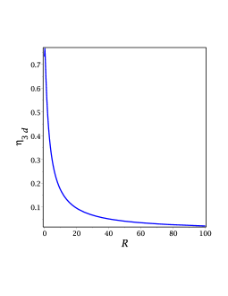
Figure 1: Stability of $3D$ gravastars in massive gravity. We have chosen $\Lambda=-0.1$, $m=1$, $c_{1}=0.1$, $C=0.1$, $R=1$, $A=0$ and $m_{0}=0.01$.

III.5 Some Features of Intermediate Thin Shell of $3D$ Gravastars

This section aims to examine the impact of massive parameter on $3D$ gravastar’s physical properties in the presence of massive gravity. In this context, we examine the proper length of the thin shell and the energy of the relativistic structure of $3D$ gravastars in massive gravity. Then, we will calculate the entropy of the thin shell of $3D$ gravastars in this theory of gravity, too. Also, we will present our results through diagrams.

III.5.1 Proper Length of the Thin Shell

Since the radius of an interior region of gravastar is $r_{1}=R$, while the radius of the exterior region is $r_{2}=R+\epsilon$, where $\epsilon$ is the thickness of the intermediate thin shell which is assumed to be very small (i.e., $\epsilon<<1$). So, the stiff perfect fluid propagates between two boundaries of the thin shell region of the gravastar. Now, the proper thickness between two surfaces can be described mathematically as 29f ; 30f

$$l=\int_{R}^{R+\epsilon}\sqrt{\frac{1}{g(r)}}dr,$$ (32)

whereas in the shell region, the expression of $g(r)$ is complicated, so the analytic solution of the above expression is not possible. So, we will solve it by numerical method and examine the behavior of massive parameters. let us assume $\sqrt{\frac{1}{g(r)}}=\frac{dF(r)}{dr}$, based on the integral above, we can write

$$l = \int_{R}^{R+\epsilon}\frac{dF(r)}{dr}dr=[F(R+\epsilon)-F(R)]$$ (33)

$$\approx \epsilon\frac{dF(r)}{dr}\mid_{R}=\epsilon\sqrt{\frac{1}{g(r)}}\mid_{R}.$$

Since $\epsilon<<1$, so $O(\epsilon^{2})\approx 0$. Therefore in the above manipulation, we considere only the first-order term of $\epsilon$. Thus for this approximation, the proper length will be

$$l\approx\frac{\epsilon}{\sqrt{B+2\Lambda R^{2}-2m^{2}c_{1}CR}}.$$ (34)

The above result shows that the proper length of the thin shell of $3D$ gravastar in massive gravity is proportional to the thickness $\epsilon$ of the shell. We observe that the proper length of the thin shell depends on the massive parameters as well. The behavior of the shell length against its thickness for different values of $m^{2}c_{1}$ and $C$ is shown in Fig. 2 and Fig. 3, respectively.

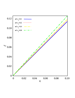
Figure 2: Proper length $l$ of the shell vs thickness of the shell $\epsilon$ for different values of $m^{2}c_{1}$. We have chosen $\Lambda=-0.1$, $C=0.1$, $R=1$ and $B=1$.

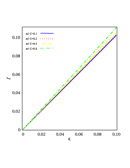
Figure 3: Proper length $l$ of the shell vs thickness of the shell $\epsilon$ for different values of $m^{2}C$. We have chosen $\Lambda=-0.1$, $c_{1}=0.1$, $R=1$ and $B=1$.

Our results in the above figures show that there is a linear relationship between the proper length and thickness of the shell, while the proper length of the system tends to increase by increasing the corresponding $m^{2}c_{1}$, and $C$ values.

III.5.2 Energy

The energy content within the shell region of $3D$ gravastar is given as 29f ; 30f

$$E=2\pi\int_{R}^{R+\epsilon}\rho rdr.$$ (35)

By expanding $F(R+\epsilon)$ binomially about $R$ and taking first order of $\epsilon$, we get

$$E\approx\frac{2\pi\epsilon p_{0}R^{2}}{2\Lambda R-m^{2}c_{1}C}.$$ (36)

The behavior of the shell energy against its thickness for different values of $m^{2}c_{1}$ and $C$ is shown in Fig. 4 and Fig. 5, respectively.

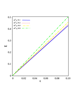
Figure 4: Energy $E$ with thickness of the shell $\epsilon$ for different values of $m^{2}c_{1}$. We have chosen $\Lambda=-0.1$, $C=0.1$, $R=1$ and $P_{0}=1$.

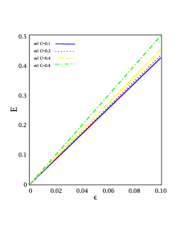
Figure 5: Energy $E$ vs thickness of the shell $\epsilon$ for different values of $m^{2}C$. We have chosen $\Lambda=-0.1$, $c_{1}=0.1$, $R=1$ and $P_{0}=1$.

The results in Fig. 4 and Fig. 5 reveal the same behavior for the shell energy. In other words, there is a linear relationship between the energy and the thickness of the shell. In addition, this energy of the system increases by increasing $m^{2}c_{1}$, and $C$, similar to the proper length of the thin shell.

III.5.3 Entropy

Mazur and Mottola have shown that the entropy density in the interior region of the gravastar is zero 29f ; 30f . To calculate the entropy relation for the shell of $3D$ gravastar, we need to use the following equation 29f ; 30f ,

$$S=\int_{R}^{R+\epsilon}4\pi r^{2}s(r)\sqrt{\frac{1}{g(r)}}dr,$$ (37)

where $s(r)$, describes the entropy density corresponding to a specific temperature $T(r)$, is given by

$$s(r)=\frac{\alpha^{2}k_{B}^{2}T(r)}{4\pi\hbar^{2}}.$$ (38)

Here $\alpha^{2}$ is a dimensionless constant, due to the fact that we are using Planck units $(K_{B}=\hbar=1)$ in our computation. Using Eqs. (37) and (38), the entropy inside a thin shell of $3D$ gravastar in massive gravity can be written as

$$S=\frac{\alpha k_{B}\sqrt{2\pi p_{0}}\int_{R}^{R+\epsilon}\frac{rdr}{\sqrt{(B+2\Lambda r^{2}-2m^{2}c_{1}Cr)(2\Lambda-\frac{m^{2}c_{1}C}{r})}}}{\hbar}.$$ (39)

By expanding $F(R+\epsilon)$ binomially about $R$ and taking the first order of $\epsilon$, we get

$$S\approx\frac{\alpha k_{B}\sqrt{2\pi p_{0}}\epsilon R}{\hbar\sqrt{(B+2\Lambda R^{2}-2m^{2}c_{1}CR)(2\Lambda-\frac{m^{2}c_{1}C}{R})}}.$$ (40)

The behavior of shell entropy against its thickness for different values of $m^{2}c_{1}$ and $C$ is shown in Fig. 6 and Fig. 7, respectively.

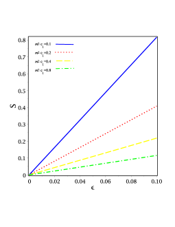
Figure 6: Entropy $S$ vs thickness of the shell $\epsilon$ for different values of $m^{2}c_{1}$. We have chosen $\Lambda=-0.1$, $C=1$, $R=1$, $P_{0}=1$ and $B=1$.

Figure 7: Entropy $S$ vs thickness of the shell $\epsilon$ for different values of $m^{2}C$. We have chosen $\Lambda=-0.1$, $c_{1}=1$, $R=1$, $P_{0}=1$ and $B=1$.

Fig. 6 and Fig. 7 show the linear relationship between entropy and thickness of the shell of $3D$ gravastars. Also, the entropy of the system decreases by increasing $m^{2}c_{1}$ and $C$.

It is notable that the mass of graviton, one of the physical principles of massive gravity, causes such a sensitive effect on astrophysical consequences such as proper length, energy, and entropy.

IV CONCLUSION

In this work, we have investigated a new model of $3D$ gravastar with an isotropic matter distribution AdS spacetime in massive gravity. Gravastars are the same gravitational vacuum stars that define a new idea in the gravitational system. Gravastar consists of three regions, the first is the inner region, the second is the middle thin shell with a thickness of $\epsilon$, and the third is the outer region. Each of these regions is described and investigated by a specific EoS. We found a set of singularity-free solutions of gravastars and hence interesting results that can be viewed as alternatives to BTZ black holes in massive gravity. In the interior region, we observed that the spacetime is the free singularity. The physical parameters, such as density, pressure, and gravitational mass in no way are dependent on the massive parameters ($m^{2}c_{1}$, and $C$) in the interior region, but the quantities $g(r)$ and $f(r)$ depend on the massive parameters. The exterior region with EOS $p=\rho=0$ is defined by the static BTZ black hole in massive gravity, which can be seen in Eq. (21). At the junction interface, the interior region joins with the exterior region with smooth matching at $r=R$. We derived some aspects like surface energy density, surface pressure, EoS, and stability. The EoS parameter depends upon the massive parameters, mass, and radius of the metric. Fig. 1 describes the stability of $3D$ gravastar structures in massive gravity. It was not easy to find the exact solution in the shell region with EoS, $p=\rho$. For this purpose, we used the thin shell approximation as $0<g(r)\equiv h<<1$ to extract the proper length, energy, and entropy for the shell region. Figs. 2, and 3 are plotted between the proper length of the shell and the thickness of the shell. These figures indicate the linear relationship between the proper length, and thickness of the shell, while the proper length of the system increases by increasing $m^{2}c_{1}$, and $C$. Our results in Figs. 4, and 5 reveal that the energy and thickness of the shell are directly proportional to each other, and also, the energy of the system increases by increasing the value of $m^{2}c_{1}$ and $C$. To see the role of entropy, thickness, and massive parameters, we drew Fig. 6, and Fig. 7. These figures indicate that there is a linear relationship between entropy and the thickness of the shell as well. In addition, the entropy of the system decreases by increasing $m^{2}c_{1}$ and $C$.

- (1) B. P. Abbott et al. (LIGO Scientific and Virgo Collaborations), Phys. Rev. Lett. 116, 061102 (2016).
- (2) B. P. Abbott et al. (LIGO Scientific and Virgo Collaborations), Phys. Rev. Lett. 116, 221101 (2016).
- (3) L. S. Finn and P. J. Sutton, Phys. Rev. D 65, 044022 (2002).
- (4) A. Gruzinov, New Astron. 10, 311 (2005).
- (5) A. S. Goldhaber and M. M. Nieto, Rev. Mod. Phys. 82, 939 (2010).
- (6) J. B. Jimenez, F. Piazza, and H. Velten, Phys. Rev. Lett. 116, 061101 (2016).
- (7) C. de Rham, J. T. Deskins, A. J. Tolley, and S.-Y. Zhou, Rev. Mod. Phys. 89, 025004 (2017).
- (8) K. Hinterbichler, Rev. Mod. Phys. 84, 671 (2012).
- (9) W. Pauli, and M. Fierz, Phys. 12, 297 (1939).
- (10) W. Pauli, and M. Fierz, Phys. 12, 3 (1939).
- (11) H. van Dam, and M. J. G. Veltman, Nucl. Phys. B 22, 397 (1970).
- (12) V. I. Zakharov, JETP Lett. 12, 312 (1970).
- (13) Y. Iwasaki, Phys. Rev. D 2, 2255 (1970).
- (14) A. I. Vainshtein, Phys. Lett. B 39, 393 (1972) .
- (15) E. Babichev, and C. Deffayet, Class. Quantum Gravit. 30, 184001 (2013).
- (16) D. G. Boulware, and S. Deser, Phys. Rev. D 6, 3368 (1972).
- (17) C. de Rham, G. Gabadadze, and A. J. Tolley, Phys. Rev. Lett. 106, 231101 (2011).
- (18) C. de Rham, and G. Gabadadze, Phys. Rev. D 82, 044020 (2010).
- (19) S. F. Hassan, R. A. Rosen, and A. Schmidt-May, JHEP 1202, 026 (2012).
- (20) S. F. Hassan, A. Schmidt-May and M. von Strauss, Phys. Lett. B 715, 335 (2012).
- (21) S. F. Hassan, and R. A. Rosen, Phys. Rev. Lett. 108, 041101 (2012).
- (22) D. Vegh, [arXiv:1301.0537].
- (23) M. Fasiello, and A. J. Tolley, JCAP 12, 002 (2013).
- (24) Y. -F. Cai, D. A. Easson, C. Gao, and E. N. Saridakis, Phys. Rev. D 87, 064001 (2013).
- (25) K. Bamba, M. W. Hossain, R. Myrzakulov, S. Nojiri, and M. Sami, Phys. Rev. D 89, 083518 (2014).
- (26) Y. -F. Cai, and E. N. Saridakis, Phys. Rev. D 90, 063528 (2014).
- (27) G. Goon, A. E. Gumrukcuoglu, K. Hinterbichler, S. Mukohyama, and M. Trodden, JCAP 08, 008 (2014).
- (28) L. Heisenberg, R. Kimura, and K. Yamamoto, Phys. Rev. D 89, 103008 (2014).
- (29) H. Kodama, and I. Arraut, Prog. Theor. Exp. Phys. 2014, 023E02 (2014).
- (30) E. Babichev, and A. Fabbri, Phys. Rev. D 90, 084019 (2014).
- (31) A. R. Solomon, J. Enander, Y. Akrami, T. S. Koivisto, F. Konnig, and E. Mortsell, JCAP 04, 027 (2015).
- (32) S. Pan, and S. Chakraborty, Ann. Phys. 360, 180 (2015).
- (33) E. Babichev, and R. Brito, Class. Quantum Gravit. 32, 154001 (2015).
- (34) S. H. Hendi, B. Eslam Panah, and S. Panahiyan, JHEP 11, 157 (2015).
- (35) A. J. Tolley, D. J. Wu, and S. Y. Zhou, Phys. Rev. D 92, 124063 (2015).
- (36) S. H. Hendi, B. Eslam Panah, and S. Panahiyan, Class. Quantum Gravit. 33, 235007 (2016).
- (37) S. H. Hendi, B. Eslam Panah, and S. Panahiyan, JHEP 2016, 29 (2016).
- (38) P. Li, X. -Z. Li, and P. Xi, Phys. Rev. D 93, 064040 (2016).
- (39) S. H. Hendi, S. Panahiyan, and B. Eslam Panah, JHEP 01, 129 (2016).
- (40) D. J. Wu, and S. Y. Zhou, Phys. Lett. B 757, 324 (2016).
- (41) S. H. Hendi, S. Panahiyan, B. Eslam Panah, and M. Momennia, Ann. Phys. (Berl.) 528, 819 (2016).
- (42) D. C. Zou, R. Yue, and M. Zhang, Eur. Phys. J. C 77, 256 (2017).
- (43) S. H. Hendi, G. H. Bordbar, B. Eslam Panah, and S. Panahiyan, JCAP 07, 004 (2017).
- (44) B. Eslam Panah, and H. L. Liu, Phys. Rev. D 99, 104074 (2019).
- (45) Y. Akrami, T. S. Koivisto, and M. Sandstad, JHEP 03, 99 (2013).
- (46) Y. Akrami, S. F. Hassan, F. Knnig, A. Schmidt-May, and A. R. Solomon, Phys. Lett. B 748, 37 (2015).
- (47) S. Panpanich, and P. Burikham, Phys. Rev. D 98, 064008 (2018).
- (48) E. Babichev, et al., Phys. Rev. D 94, 084055 (2016).
- (49) E. Babichev, et al., JCAP 09, 016 (2016).
- (50) B. Eslam Panah, S. H. Hendi, and Y. C. Ong, Phys. Dark Universe. 27, 100452 (2020).
- (51) M. -S. Hou, H. Xu, and Y. C. Ong, Eur. Phys. J. C 80, 1090 (2020).
- (52) J. Xu, L. M. Cao, and Y. P. Hu, Phys. Rev. D 91, 124033 (2015).
- (53) S. H. Hendi, R. B. Mann, S. Panahiyan, and B. Eslam Panah, Phys. Rev. D 95, 021501(R) (2017).
- (54) A. Dehghani, S. H. Hendi, and R. B. Mann, Phys. Rev. D 101, 084026 (2020).
- (55) P. Mazur, and E. Mottola, Universe. 9, 88 (2023).
- (56) P. Mazur, and E. Mottola, Proc. Natl. Acad. Sci. 101, 9545 (2004).
- (57) Z. Yousaf, K. Bamba, M. Z. Bhatt, and U. Ghafoor, Phys. Rev. D 100, 024062 (2019).
- (58) M. Visser, and D. L. Wiltshire, Class. Quantum Gravit. 21, 1135 (2004).
- (59) C. Cattoen, T. Faber, and M. Visser, Class. Quantum Gravit. 22, 4189 (2005).
- (60) B. M. N. Carter, Class. Quantum Gravit. 22, 4551 (2005).
- (61) D. Horvat, S. Ilijic, and A. Marunovic, Class. Quantum Gravit. 26, 025003 (2009).
- (62) B. V. Turimov, B. J. Ahmedov, and A. A. Abdujabbarov, Mod. Phys. Lett. A 24, 733 (2009).
- (63) G. ’t Hooft, NATO Sci. Ser. B 59, 135 (1980).
- (64) M. Dine, Ann. Rev. Nucl. Part. Sci. 65, 43 (2015).
- (65) S. Carlip, Living Rev. Relativ. 8, 1 (2005).
- (66) J. J. van der Bij, R. D. Pisarski, and S. Rao, Phys. Lett. B 179, 87 (1986).
- (67) E. J. Copeland, and T. W. B. Kibble, Proc. R. Soc. A 466, 623 (2010).
- (68) J. J. Blanco-Pillado, K. D. Olum, and X. Siemens, Phys. Lett. B 778, 392 (2018).
- (69) J. P. Luminet, Universe. 2, 1 (2016).
- (70) J. J. van der Bij, Phys. Rev. D 76, 121702 (2007).
- (71) J. J. van der Bij, Gen. Relativ. Gravit. 43, 2499 (2011).
- (72) M. Banados, C. Teitelboim, and J. Zanelli, Phys. Rev. Lett. 69, 1849(1992) .
- (73) A. Larranaga, Turk. J. Phys. 32, 1 (2008).
- (74) M. Cadoni, and C. Monni, Phys. Rev. D 80, 024034 (2009) .
- (75) M. Akbar, H. Quevedo, K. Saifullah, A. Sanchez, and S. Taj, Phys. Rev. D 83, 084031 (2011).
- (76) S. Carlip, Class. Quantum Gravit. 12, 2853 (1995).
- (77) A. Ashtekar, J. Wisniewski, and O. Dreyer, Adv. Theor. Math. Phys. 6, 507 (2003) .
- (78) T. Sarkar, G. Sengupta, and B. Nath Tiwari, JHEP 11, 015 (2006).
- (79) E. Witten, ”Three-Dimensional Gravity Revisited”, [arXiv:0706.3359].
- (80) E. Witten, Adv. Theor. Math. Phys. 2, 505 (1998).
- (81) A. Larranaga, Commun. Theor. Phys. 50, 1341 (2008).
- (82) H. W. Lee, Y. S. Myung, and J. Y. Kim, Phys. Lett. B 466, 211 (1999).
- (83) M. A. Anacleto, F. A. Brito, and E. Passos, Phys. Lett. B 743, 184 (2015).
- (84) R. Emparan, G. T. Horowitz, and R. C. Myers, JHEP 01, 021 (2000).
- (85) M. R. Setare, Eur. Phys. J. C 49, 865 (2007).
- (86) S. Carlip, Class. Quantum Gravit. 22, 85 (2005).
- (87) P. Caputa, V. Jejjala, and H. Soltanpanahi, Phys. Rev. D 89, 046006 (2014).
- (88) E. Frodden, M. Geiller, K. Noui, and A. Perez, JHEP 05, 139 (2013).
- (89) D. V. Singh, and S. Siwach, Class. Quantum Gravit. 30, 235034 (2013).
- (90) F. Rahaman, A. A. Usmani, S. Ray, and S. Islam, Phys. Lett. B 717, 1 (2012).
- (91) F. Rahaman, S. Ray, A. A. Usmani, and S. Islam, Phys. Lett. B 707, 319 (2012).
- (92) F. S. N. Lobo, and R. Garattini, JHEP 12, 065 (2013).
- (93) A. A. Usmani et al., Phys. Lett. B 701, 388 (2011).
- (94) H. Barzegar, M. Bigdeli, G. H. Bordbar, and B. Eslam Panah, Eur. Phys. J. C 83, 151 (2023).
- (95) R. Emparan et al., JHEP 11, 073 (2022).
- (96) G. Darmois, Des Sciences Mathematiques XXV, Fasticule XXV (Gauthier-Villars, Paris, France, 1927), chap. V.
- (97) W. Israel, Nuovo Cimento B 44, 1 (1966).
- (98) W. Israel, Nuovo Cimento B 48, 463 (1967).
- (99) A. A. Usmani et al., Gen. Relativ. Gravit. 42, 2901 (2010).
- (100) F. Rahaman, K. A. Rahman, Sk. A Rakib, and P. K. F. Kuhfittig, Int. J. Theor. Phys. 49, 2364 (2010).
- (101) F. Rahaman et al., Gen. Relativ. Gravit. 38, 1687 (2006).
- (102) F. Rahaman et al., Class. Quantum Gravit. 28, 155021 (2011).
- (103) G. P. Perry, and R. B. Mann, Gen. Relativ. Gravit. 24, 305 (1992).
- (104) C. Bejarano, E. F. Eiroa, and C. Simeone, Eur. Phys. J. C 74, 3015 (2014).
- (105) E. Poisson, M. Visserti, Phys. Rev. D 52, 12 (1995).
- (106) U. Debnath, Eur. Phys. J. C 136, 442 (2021).
- (107) F. S. N. Lobo, and P. Crawford, Class. Quantum Gravit. 21, 391 (2004)