Impact of Property Covariance on Cluster Weak lensing Scaling Relations

Abstract

We present an investigation into a hitherto unexplored systematic that affects the accuracy of galaxy cluster mass estimates with weak gravitational lensing. Specifically, we study the covariance between the weak lensing signal, $\Delta\Sigma$, and the “true” cluster galaxy number count, $N_{\rm gal}$, as measured within a spherical volume that is void of projection effects. By quantifying the impact of this covariance on mass calibration, this work reveals a significant source of systematic uncertainty. Using the MDPL2 simulation with galaxies traced by the SAGE semi-analytic model, we measure the intrinsic property covariance between these observables within the 3D vicinity of the cluster, spanning a range of dynamical mass and redshift values relevant for optical cluster surveys. Our results reveal a negative covariance at small radial scales ($R\lesssim R_{\rm 200c}$) and a null covariance at large scales ($R\gtrsim R_{\rm 200c}$) across most mass and redshift bins. We also find that this covariance results in a $2-3\%$ bias in the halo mass estimates in most bins. Furthermore, by modeling $N_{\rm gal}$ and $\Delta\Sigma$ as multi-(log)-linear equations of secondary halo properties, we provide a quantitative explanation for the physical origin of the negative covariance at small scales. Specifically, we demonstrate that the $N_{\rm gal}$–$\Delta\Sigma$ covariance can be explained by the secondary properties of halos that probe their formation history. We attribute the difference between our results and the positive bias seen in other works with (mock)-cluster finders to projection effects. These findings highlight the importance of accounting for the covariance between observables in cluster mass estimation, which is crucial for obtaining accurate constraints on cosmological parameters.

1 Introduction

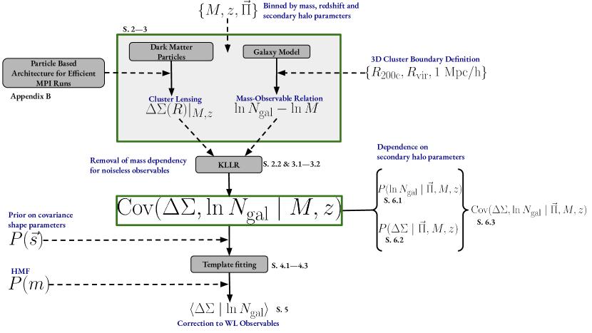
Figure 1: Graphic representation of the modeling of $\text{Cov}(\Delta\Sigma,\ln N_{\rm gal}\mid M,z)$ — the covariance between the halo weak lensing signal $\Delta\Sigma(R)$ and log-richness $\ln N_{\rm gal}$ conditioned on mass and redshift — and its dependence with secondary halo parameters $\Pi$. The labels marked S. XX point to the location in the text. A full list of the notations used in this paper is introduced in Table 1 & 2.

Cluster abundance and its evolution with redshift are linked to the constituents of the Universe through the growth of cosmic structure. (Allen et al., 2011, for a review). Cluster abundance measured in large-scale galaxy surveys offers power constraints on cosmological parameters (e.g., Vikhlinin et al., 2009; Mantz et al., 2015; de Haan et al., 2016; Mantz et al., 2016a; Dark Energy Survey Collaboration et al., 2016; Pierre et al., 2016; Costanzi et al., 2021). These constraints are based on accurate cluster mass measurements, which are not directly observable and must be inferred. Cluster mass calibration has been identified as one of the leading systematic uncertainties in cosmological constraints using galaxy cluster abundance (Mantz et al., 2010; Rozo et al., 2010; von der Linden et al., 2014; Applegate et al., 2014; Dodelson et al., 2016; Murata et al., 2019; Costanzi et al., 2021). Accurate mappings between a population of massive clusters and their observables are thus critical and essential in cluster cosmology. Considerable effort has been put into measuring the statistical relationships between masses and observable properties that reflect their baryon contents (see Giodini et al., 2013, for a review) and quantifying the sources of uncertainties.

The Dark Energy Survey (DES) cluster cosmology from the Year 1 dataset (Costanzi et al., 2021) reported tension in $\Omega_{m}$ — the mean matter density of the universe — with the DES 3x2pt probe that utilizes three two-point functions from the DES galaxy survey (Abbott et al., 2018). The tension between these two probes that utilize the same underlying dataset may be attributed to systematics that bias the weak lensing mass of clusters low at the low mass end (To et al., 2021; Costanzi et al., 2021). Similarly, there is a discrepancy in the measurements of matter density fluctuations between the cosmic microwave background (CMB) measurements and late-time cosmological probes such as cluster abundances (Planck Collaboration et al., 2020; Qu et al., 2023). Commonly referred to as the “$S_{8}$” tension, a possible origin for this discrepancy is that cluster masses are biased low (Blanchard & Ilić, 2021) due to systematics in cluster mass calibration. On the other hand, the tension can also originate from new physics that extends the Standard Cosmological model. Thus, it is important to understand the systematics of cluster mass calibration. Cluster masses estimated from X-ray and SZ data are known to suffer from hydrostatic bias (Pratt et al., 2019). Conversely, cluster masses estimated from weak lensing have the potential to be more accurate compared to X-ray and SZ cluster masses. The systematics in the weak lensing mass calibration has just started to be explored recently (Applegate et al., 2014; Schrabback et al., 2018; McClintock et al., 2019; Kiiveri et al., 2021; Wu et al., 2022).

A relatively unexplored category of cluster systematics is the covariance between different cluster properties, including cluster observables and mass proxies. In cluster mass calibration, it is often assumed that this property covariance is negligible. However, as initially pointed out by Nord et al. (2008) and later shown in Evrard et al. (2014) and Farahi et al. (2018), non-zero property covariances between cluster observables can induce non-trivial, additive bias in cluster mass. As property covariance is additive, the systematic uncertainties that it induces will not be mitigated with the reduction of statistical errors as the sample size of the cluster increases. To achieve accurate cosmological constraints with the next generation of large-scale cluster surveys, it is imperative that systematic uncertainties in the property covariance be accurately and precisely quantified (Rozo et al., 2014).

Although the property covariance linking mass to observable properties is becoming better understood and measured (Wu et al., 2015; Mantz et al., 2016a; Farahi et al., 2018; Farahi et al., 2019; Sereno et al., 2020), studies that specifically investigate weak lensing property covariance are scarce, which poses a challenge for upcoming lensing surveys of galaxy clusters such as the Rubin (Ivezić et al., 2019) observatories. To achieve the percentage-level lensing mass calibration goals for the upcoming observations, the property covariance of weak lensing must be quantified.

The physical origins of property covariance in lensing signals of galaxy clusters can be attributed to the halo formation history of the cluster and baryonic physics (Xhakaj et al., 2022). Developing a first-principle physical model for the property covariance as a function of halo formation history and baryonic physics is a daunting task due to the highly non-linear and multi-scale physics involved in cluster formation. To make progress, in this paper, we adopt a simulation-based, data-driven approach whereby we develop semi-analytical parametric models of property covariance, which we then calibrate with cosmological simulations. We then apply our model to quantify the bias induced due to a non-zero property covariance in the expected weak lensing signal and the mass-observable scaling relation.

As will be presented in §3, a key element of this analysis is the estimation of true cluster richness by encircling clusters within a 3D radius within the physical vicinity of the halo center, as opposed to a 2D projected radius used by cluster finders as redMaPPer (Rykoff et al., 2014a) by identifying galaxies within the red-sequence band in the color-magnitude space — the major difference being the removal of projection effects, or the mis-identification of non-cluster galaxies in the 2D projected radius from the photometric redshift uncertainty of the red-sequence when estimating the true richness from a gravitationally bound region around the halo. Furthermore, as this simulation-based study does not introduce other observational systematics as shape noise of galaxies, point spread function, miscentering etc., this study can be used to explore the intrinsic covariance between observables prior to the addition of extrinsic systematics as projection effects. Our results will not only provide insight into the physical origin of the covariance, the difference between the total covariance as measured by observations and the intrinsic covariance will provide estimates on the amplitude of the extrinsic component.

The goals of this work are to (i) develop an analytical model that accounts for and quantifies the effect of non-zero covariance on cluster mass calibration, (ii) quantify this property covariance utilizing cosmological simulations, (iii) update uncertainties on inferred cluster mass estimates, and (iv) explain the physical origin of the covariance using secondary halo parameters. The rest of this paper is organized as follows. In §2, we present a population-based analytical framework. In §3, we describe the simulations and data-vector employed in this work. In §4, we present our measurements and the covariance model. In §5, we present the impact of the covariance on weak lensing mass calibration. In §6, we quantify the physical origin of the covariance by parameterizing it using secondary halo parameters. In §7, we compare our work with those that employ realistic cluster finders. we conclude in §8.

2 Theoretical Framework

This section presents a theoretical framework that examines the impact of covariance on mass-observable scaling relations. In §2.1 we introduce the definitions of richness and weak lensing excess surface mass density and their scaling relations with cluster mass. We then describe the model of property covariance of richness and excess surface mass density in §2.2. In §2.3, we model the impact of covariance on stacked observable scaling relations. Finally, in §2.4, we develop a theoretical framework that explains the covariance based on a set of secondary halo parameters. A graphic representation of the outline of the paper is shown in Figure 1.

Table 1: Notations employed in our framework for the covariance in §2.3

Parameter	Explanation
$\Delta\Sigma$	Weak lensing signal
$M$	halo mass in $M_{\odot}h^{-1}$
$N_{\rm gal}$	optical richness enclosed inside 3D radius
$z$	redshift
$r_{p}$	projected and normalised radius

Table 2: Scaling Relation Conventions.

Parameter	Explanation
$\pi_{a}$	normalization in scaling relation $\langle a\mid M\rangle$
$\alpha_{a}$	slope in scaling relation $\langle a\mid M\rangle$
$\sigma_{a}$	scatter about $\langle a\mid M\rangle$
$r_{a,b}$	correlation between $a$ and $b$ at fixed $M$
$\pi_{a\mid b}$	normalisation in scaling relation $\langle a\mid b\rangle$
$\alpha_{a\mid b}$	slope in scaling relation $\langle a\mid b\rangle$
$\sigma_{a\mid b}$	scatter about $\langle a\mid b\rangle$
$a,b$	$a,b\in\{\Delta\Sigma,\ln N_{\rm gal}\}$

2.1 Observable-Mass Relations

2.1.1 Excess Surface Mass Density $\Delta\Sigma$ from Weak Lensing

In weak lensing measurements of galaxy clusters, the key observable is the excess surface mass density, denoted $\Delta\Sigma$. The excess surface mass density is defined as

$$\Delta\Sigma(M,z,r_{p})=\overline{\Sigma}(M,z,<r_{p})-\Sigma(M,z,r_{p}),$$ (1)

where $\overline{\Sigma}(M,z,<r_{p})$ denotes the average surface mass density within projected radius $r_{p}$, and $\Sigma(M,z,r_{p})$ represents the average of the surface mass density at $r_{p}$. We model the average surface mass density $\Sigma$ as

$$\Sigma(r_{p})=\rho_{m}\int^{+\infty}_{-\infty}\Bigg{(}1+\xi_{hm}\Big{(}r=\sqrt{r_{p}^{2}+z^{2}}\Big{)}\Bigg{)}dz,$$ (2)

where $\rho_{m}$ is the mean matter density at the redshift of the cluster, $R$ is the projected radius in the plane of the sky, $z$ is the length along the line of sight, and $\xi_{hm}(r)$ is the halo-matter correlation function which characterises the total mass density within a halo. Under the halo model, the halo-matter correlation function consists of a “one-halo” term:

$$\xi_{\rm 1h}(r|M)=\frac{\rho_{\rm NFW}(r|M)}{\rho_{m0}}-1,$$ (3)

and a “two-halo" term:

$$\xi_{\rm 2h}(r|M)=b^{2}(M)\xi_{\rm lin}(r),$$ (4)

where $\rho_{\rm NFW}$ is the NFW density profile, and $\xi_{\rm lin}$ is the linear matter correlation function, and $b$ is the halo bias parameter.

In weak lensing, the excess surface density $\Delta\Sigma$ is tied to the tangential shear $\gamma_{t}$ of the galaxies relative to the center of each foreground halo by the relation

$$\Sigma_{\rm crit}\gamma_{t}=\overline{\Sigma}(<R)-\Sigma(R)\equiv\Delta\Sigma(R),$$ (5)

where the critical surface density $\Sigma_{\rm crit}$ defined as

$$\Delta\Sigma_{\rm crit}=\frac{c^{2}}{4\pi G}\frac{D_{s}}{D_{l}D_{ls}},$$ (6)

and where $D_{s}$, $D_{l}$, and $D_{ls}$ refer to the angular diameter distances to the source, the lens, and between the lens and source, respectively.

In this work, for each halo of mass $M$ at redshift $z$, we compute the corresponding $\Delta\Sigma$ profile. We model the two-halo term using different halo bias models of Tinker et al. (2010), Pillepich et al. (2010), and Bhattacharya et al. (2011). At the transition radius between the one- and two-halo regimes, we follow SDSS (Zu et al., 2014) in setting the halo–matter correlation to the maximum value of the two terms, i.e.,

$$\xi_{hm}(r|M)=\max\{\xi_{\rm 1h}(r|M),~{}\xi_{\rm 2h}(r|M)\}.$$ (7)

In Fig. 2, the theoretical models described above are compared with our measurements of $\Delta\Sigma$ in cosmological simulations to validate our data product.

2.1.2 Optical Richness $N_{\rm gal}$

Optical richness $N_{\rm gal}$ is an observable measure of the abundance of galaxies within a galaxy cluster. It is often defined as the number of detected member galaxies brighter than a certain luminosity threshold within a given aperture or radius around the cluster centre. Richness is often used as a proxy for cluster mass, as more massive clusters are expected to have more member galaxies (e.g., Rozo et al., 2014; Rykoff et al., 2014a). The richness-mass scaling relation relates the richness of a galaxy cluster to its mass. In this work, we consider $N_{\rm gal}$-$M_{\Delta}$ scaling relation expressed as

$$\langle\ln N_{\rm gal}\mid M_{\Delta},z\rangle=\pi_{N_{\rm gal}}(M,z)+\alpha_{N_{\rm gal}}(M,z)\ln M_{\Delta}.$$ (8)

where $M_{\Delta}$ is the mass of the halo within a radius where the mean density is $\Delta$ times the critical density of the universe, $\alpha_{N_{\rm gal}}(M,z)$ is the power-law slope of the relation, $\pi_{N_{\rm gal}}(M,z)$ is a normalisation that is a function of redshift and mass.

2.1.3 Halo Mass and Radius Definitions

A common approach to defining a radial boundary of a galaxy cluster is such that the average matter density inside a given radius is the product of a reference overdensity $\Delta_{\rm ref}$ times the critical ($\rho_{c}$) or mean density ($\rho_{m}$) of the universe at that redshift. The critical density is defined as

$$\rho_{c}=\frac{3H_{0}^{2}}{8\pi G}E(z),$$ (9)

where $E(z)^{2}=\Omega_{m,0}(1+z)^{3}+\Omega_{\Lambda,0}$, $\Omega_{m,0}$ is the present day matter fraction of the universe, $\Omega_{\Lambda,0}$ is the dark energy fraction at the present age such that $\Omega_{m,0}+\Omega_{\Lambda,0}=1$ for a flat universe ignoring the minimal contribution from the radiation fraction. The mean (background) density is defined as

$$\rho_{b}=\frac{3H_{0}^{2}}{8\pi G}(\Omega_{m,0}(1+z)^{3}).$$ (10)

The overdensity $\Delta_{c}=200$ is commonly chosen as the reference overdensity in optical weak lensing studies and is closely related to the virial radius. Another radius definition is the virial radius $R_{\rm vir}$, with overdensity values calibrated from cosmological simulations (Bryan & Norman, 1998). In this work, we use $R_{\rm 200c}$ and $R_{\rm vir}$ to scale various observations, including the $\Delta\Sigma$ measurements and richness. Since the covariance is close to zero at the outskirts $R\gtrsim R_{\rm 200c}$ as shown in §4, we adopt $r_{p}=R/R_{\rm 200c}$ and $r_{p}=R/R_{\rm vir}$ as our normalised radii, as the cluster properties are more self-similar with respect to $\rho_{c}(z)$ compared to $\rho_{b}(z)$ (Diemer & Kravtsov, 2014; Lau et al., 2015). To test for the robustness of our covariance against different radii definitions, we also introduce a physical radius of a toy model of a constant $R=1$ Mpc/h; here $h=0.6777$ is the reduced Hubble constant used in this study.

2.2 Covariance between $\Delta\Sigma$ and $N_{\rm gal}$

In optical surveys, we cannot expect the covariance between richness $N_{\rm gal}$ and the excess surface mass density $\Delta\Sigma$ to be zero. Ignoring this covariance will lead to bias in cluster mass inferred from the excess surface mass density of the cluster selected based on richness. This work aims to quantify and analyse this covariance and its impact on the mass calibration relation. To achieve this objective, we must first specify the joint probability distribution of excess surface mass density and richness, $p(\Delta\Sigma,\ln N_{\rm gal}\mid M,z,r_{p})$. In this work, we assume that the joint distribution follows a multivariate normal distribution (Stanek et al., 2010; Evrard et al., 2014; Mulroy et al., 2019; Miyatake et al., 2022), which is fully specified with two components, the mean vector and the property covariance.

The mean vectors here are the scaling relations of the expected richness $\langle\ln N_{\rm gal}\mid M,z\rangle$ and weak lensing signal $\langle\Delta\Sigma\mid M,z,r_{p}\rangle$ at fixed mass $M$, redshift $z$, and projected radius $r_{p}$ with cluster mass are given by

$$\langle\ln N_{\rm gal}\mid M,z\rangle = \pi_{N_{\rm gal}}(M,z)+\alpha_{N_{\rm gal}}(M,z)\ln M,$$ (11)

$$\langle\Delta\Sigma\mid M,z,r_{p}\rangle = \pi_{\Delta\Sigma}(M,r_{p},z)+\alpha_{\Delta\Sigma}(M,r_{p},z)\ln M,$$ (12)

where $\alpha_{i}$ is the power-law slope of the relation and $\pi_{i}$ is a normalization that is a function of redshift and mass, for $i\in\{\Delta\Sigma,\ln N_{\rm gal}\}$.

From these mean relations, the scaling between these two observables can be modeled as a local linear relation where the slope and normalization are functions of halo mass $M$, redshift $z$, and projected radius $r_{p}$ from the halo center:

$$\langle\Delta\Sigma\mid N_{\rm gal},z,r_{p}\rangle=\pi_{\Delta\Sigma\mid N_{\rm gal}}(N_{\rm gal},z,r_{p})+\alpha_{\Delta\Sigma\mid N_{\rm gal}}(N_{\rm gal},z,r_{p})\ln N_{\rm gal},$$ (13)

where $\pi$ and $\alpha$ are the normalization and slope of the model.

The property covariance matrix is a combination of scatter and correlation between the scatter of $\Delta\Sigma$ and $\ln N_{\rm gal}$ at a fixed halo mass, redshift, and projected radius. We use $\sigma_{N_{\rm gal}}(M,z)$ and $\sigma_{\Delta\Sigma}(M,z,r_{p})$ to denote the scatter of the observable-mass relation for $\ln N_{\rm gal}$ and $\Delta\Sigma$, respectively, and use $r_{N_{\rm gal},\Delta\Sigma}(M,z,r_{p})$ to denote the correlation between these scatters. The covariance matrix is then given by

$${\rm Cov}_{i,j}(M,z,r_{p})=r_{i,j}(M,z,r_{p})\ \sigma_{i}(M,z,r_{p})\ \sigma_{j}(M,z,r_{p}),$$ (14)

where $i$ and $j\in\{\Delta\Sigma,\ln N_{\rm gal}\}$. Specifically, the covariance between $\Delta\Sigma$ and $N_{\rm gal}$ can be expressed in terms of the residuals about the mean quantities

$${\rm Cov}_{\Delta\Sigma,N_{\rm gal}}(M,z,r_{p})={\rm Cov}({\rm res}_{\Delta\Sigma}(M,z,r_{p}),{\rm res}_{N_{\rm gal}}(M,z)),$$ (15)

where the residuals of the $\Delta\Sigma$ and $N_{\rm gal}$ are, respectively, are given by

$${\rm res}_{\Delta\Sigma}(M,z,r_{p})=\Delta\Sigma-\langle\Delta\Sigma\mid M,z,r_{p}\rangle,$$ (16)

$${\rm res}_{N_{\rm gal}}(M,z)=\ln N_{\rm gal}-\langle\ln N_{\rm gal}\mid M,z\rangle.$$ (17)

To model the mass dependencies of the mean profiles of $\Delta\Sigma$ and $\ln N_{\rm gal}$, we employ the Kernel Localised Linear Regression (KLLR, Farahi et al., 2022a) method. This regression method fits a locally linear model while capturing globally non-linear trends in data has shown to be effective in modelling halo mass dependencies in scaling relations (Farahi et al., 2018; Wu et al., 2022; Anbajagane et al., 2022). By developing a local-linear model of $\Delta\Sigma-\ln N_{\rm gal}$ with respect to the halo mass and computing the residuals about the mean relation, we remove bias in the scatter due to mass dependence and reduce the overall size of the scatter.

2.3 Corrections to the $\Delta\Sigma-N_{\rm gal}$ relation due to Covariance

The shape of the halo mass function plays an important role in evaluating the conditional mean value of $\langle\Delta\Sigma\mid N_{\rm gal},z,r_{p}\rangle$ where the scatter between two observables with a fixed halo mass is correlated. This is also true when the observables are the excess surface mass density $\Delta\Sigma$ and the richness $N_{\rm gal}$. Ignoring the contribution from the correlated scatter, to the zeroth order, the expected $\Delta\Sigma$ evaluated at fixed richness is

$$\langle\Delta\Sigma\mid N_{\rm gal},z\rangle_{0}=\pi_{\Delta\Sigma}+\alpha_{\Delta\Sigma}\langle\ln M\mid N_{\rm gal}\rangle,$$ (18)

where $\langle\ln M\mid N_{\rm gal}\rangle$ is the mass-richness scaling relation. Here $\alpha_{\Delta\Sigma}$ and $\pi_{\Delta\Sigma}$ are evaluated at $\ln N_{\rm gal}$. This is the model that has been used in mass calibration with stacked weak lensing profiles (Johnston et al., 2007; Kettula et al., 2015; McClintock et al., 2019; Chiu et al., 2020; Lesci et al., 2022).

The first- and second-order approximations of the scaling relation are given by

$$\langle\Delta\Sigma\mid N_{\rm gal},z\rangle_{1} =\langle\Delta\Sigma\mid N_{\rm gal},z\rangle_{0}+\frac{\gamma_{1}}{\alpha_{N_{\rm gal}}}\times{\rm Cov}(\Delta\Sigma,\ln N_{\rm gal}),$$ (19)

and

$$\langle\Delta\Sigma |N_{\rm gal},z\rangle_{2}=\langle\Delta\Sigma\mid N_{\rm gal},z\rangle_{\rm fid}+$$ (20)

$${\rm Cov}(\Delta\Sigma,\ln N_{\rm gal})\times\Big{[}\frac{x_{s}}{\alpha^{2}_{N_{\rm gal}}}(\alpha_{N_{\rm gal}}\gamma_{1}+\gamma_{2}(\ln N_{\rm gal}-\pi_{N_{\rm gal}}))\Big{]},$$

where $\langle\Delta\Sigma\mid N_{\rm gal},z\rangle_{\rm fid}$ is the fiducial relation taking into account the curvature of the HMF but independent of the covariance; $x_{s}=(1+\gamma_{2}\sigma^{2}_{M|N_{\rm gal},1})^{-1}$ is the compression factor due to curvature of the HMF, the subscript 1 denoting that the scatter is taken from the HMF expanded to first order; here we omit the $(M,z)$ dependence of the covariance as a shorthand notation.

Here $\gamma_{1}$ and $\gamma_{2}$ are the parameters for the first and second-order approximations to the mass dependence of the halo mass function (e.g., Evrard et al., 2014):

$$\frac{{\rm d}n_{\rm hmf}(M,z)}{{\rm d}\ln M}\approx A(z)\exp\left[-\gamma_{1}(M,z)\ln M-\frac{1}{2}\gamma_{2}(M,z)(\ln M)^{2}\right].$$ (21)

where $A(z)$ is the normalisation of the mass function due to the redshift alone. In deriving the above approximations, we have made use of the fact that ${{\rm Cov}}(\Delta\Sigma,\ln N_{\rm gal}|M,z)\equiv r_{\Delta\Sigma,N_{\rm gal}}\sigma_{\Delta\Sigma}\sigma_{N_{\rm gal}}$. The terms $\sigma_{\Delta\Sigma}$, $\sigma_{N_{\rm gal}}$, $r_{N_{\rm gal},\Delta\Sigma}$, $\gamma_{1}$ and $\gamma_{2}$ are evaluated at the mass implied by $\langle\ln M\mid N_{\rm gal}\rangle$.

These property covariance correction terms are absent in the current literature. A key feature of this approximation method is that the second-order solution has better than percent-level accuracy when the halo mass function is known (Farahi et al., 2016). In Figure 9, we demonstrate that the statistical uncertainties for the first-order correction in Eq. (19) is larger than the uncertainty in the halo mass function and the uncertainty induced due to the second-order halo mass approximation.

2.4 Secondary halo parameter dependence of ${\rm Cov}(\Delta\Sigma,\ln N_{\rm gal}|M,z)$

Table 3: Notations employed in exploring the secondary halo parameter dependence

Parameter	Explanation
$\Pi$	Set of secondary halo parameters
$\Gamma_{\rm inst}$	instantaneous mass accretion rate (MAR)
$\Gamma_{\rm 100Myr}$	mean MAR over the past 100 Myr
$\Gamma_{\rm dyn}$	mean MAR over virial dynamical time
$\Gamma_{\rm 2dyn}$	mean MAR over two virial dynamical time
$\Gamma_{\rm peak}$	Growth rate of peak mass from current z to z+0.5
$a_{1/2}$	Half mass scale factor
$c_{\rm vir}$	$R_{\rm vir}$ concentration
T/|U|	Absolute value of the kinetic to potential energy ratio
$X_{\rm off}$	Offset of density peak from mean particle position (kpc $h^{-1}$)

We elucidate the physical origin of the covariance between $\Delta\Sigma$ and $\ln N_{\rm gal}$ by developing a phenomenological model based on the secondary halo parameters listed in Table 3. These parameters capture the halo’s mass accretion history, which we hypothesise is the driving force behind the observed covariance. To incorporate these parameters into our model, we extend Equations (11) and (12) by introducing multi-linear terms that include the secondary halo parameters denoted by the vector $\Pi$:

$$\langle\ln N_{\rm gal}\mid\Pi,M,z\rangle =\pi_{N_{\rm gal}}(M,z)+\alpha_{N_{\rm gal}}(M,z)\ln M$$

$$+\vec{\beta}_{N_{\rm gal}}^{\intercal}(M,z)\cdot\Pi+\epsilon_{N_{\rm gal}}.$$ (22)

$$\langle\Delta\Sigma\mid\Pi,M,z\rangle =\pi_{\Delta\Sigma}(M,z)+\alpha_{\Delta\Sigma}(M,z)\ln M$$

$$+\vec{\beta}_{\Delta\Sigma}^{\intercal}(M,z)\cdot\Pi+\epsilon_{\Delta\Sigma},$$ (23)

where $\Pi$ is a vector of secondary halo parameters of potential interest listed in Table 3, and $\epsilon_{\Delta\Sigma}$ and $\epsilon_{N_{\rm gal}}$ are Gaussian white noise terms with zero means and fixed variances. Additionally, we assume $\langle\epsilon_{N_{\rm gal}}\epsilon_{\Delta\Sigma}\rangle=0$, which implies that the scatter about the mean relations is uncorrelated after factoring in the secondary properties.

Due to bilinearity and distributive properties of covariance, combining Equation (22) and (23) yields:

$$\text{Cov}(\Delta\Sigma, \ln N_{\rm gal}\mid M,z)=\text{Cov}(\langle\Delta\Sigma\rangle,\langle N_{\rm gal}\rangle)+\text{Cov}(\langle\Delta\Sigma\rangle,\vec{\beta}_{N_{\rm gal}}^{\intercal}\cdot\Pi)$$

$$\ \ +\text{Cov}(\langle\Delta\Sigma\rangle,\epsilon_{N_{\rm gal}})+\text{Cov}(\vec{\beta}_{\Delta\Sigma}^{\intercal}\cdot\Pi,\langle\ln N_{\rm gal}\rangle)$$

$$\ \ +\text{Cov}(\vec{\beta}_{\Delta\Sigma}^{\intercal}\cdot\Pi,\vec{\beta}_{N_{\rm gal}}^{\intercal}\cdot\Pi)+\text{Cov}(\vec{\beta}_{\Delta\Sigma}^{\intercal}\cdot\Pi,\epsilon_{N_{\rm gal}})$$

$$\ \ +\text{Cov}(\epsilon_{\Delta\Sigma},\langle\ln N_{\rm gal}\rangle)+\text{Cov}(\epsilon_{\Delta\Sigma},\vec{\beta}_{N_{\rm gal}}^{\intercal}\cdot\Pi)$$

$$\ \ +\text{Cov}(\epsilon_{N_{\rm gal}},\epsilon_{\Delta\Sigma}),$$ (24)

where we omit the explicit $(M,z)$ dependence in $\langle\Delta\Sigma\mid M,z\rangle$, $\langle\ln N_{\rm gal}\mid M,z\rangle$, $\vec{\beta}_{\Delta\Sigma}^{\intercal}(M,z)$, $\vec{\beta}_{N_{\rm gal}}^{\intercal}(M,z)$, $\epsilon_{N_{\rm gal}}(M,z)$ and $\epsilon_{\Delta\Sigma}(M,z)$ to simplify the notation. The KLLR method is utilised to estimate these mass-dependent parameters. All terms involving $\langle\Delta\Sigma\rangle$ and $\langle\ln N_{\rm gal}\rangle$ vanish, as these terms are independent of $\Pi$ by definition. Terms involving $\epsilon_{N_{\rm gal}}$ and $\epsilon_{\Delta\Sigma}$ also go to zero, as they are uncorrelated Gaussian scatters. Only the term ${\rm Cov}(\vec{\beta}_{\Delta\Sigma}^{\intercal}\cdot\Pi,\vec{\beta}_{N_{\rm gal}}^{\intercal}\cdot\Pi)$ remains, and hence our final expression for the covariance is

$${\rm Cov}(\Delta\Sigma,\ln N_{\rm gal}\mid M,z) ={\rm Cov}(\vec{\beta}_{\Delta\Sigma}^{\intercal}\cdot\Pi,\vec{\beta}_{N_{\rm gal}}^{\intercal}\cdot\Pi)$$ (25)

$$=\vec{\beta}_{\Delta\Sigma}^{\intercal}{\rm Cov}(\Pi,\Pi)\vec{\beta_{N_{\rm gal}}}.$$ (26)

To estimate the error in covariance due to each of the secondary halo parameters, we compute ${\rm Cov}(\Delta\Sigma,\Pi_{i}|M,z)$ for each secondary halo parameter $i$ in each ($r_{p}$, $M$, $z$) bin and take their standard deviations as the error measurement. In this way, we bypass the need to model $\Delta\Sigma$ as a linear combination of $\Pi$, and its dependence on $\Pi$ is no longer encapsulated in $\vec{\beta_{\Delta\Sigma}}$ but directly through ${\rm Cov}(\Delta\Sigma,\Pi_{i}|M,z)$. Using the same derivation as in Equation (2.4), we arrive at the expression

$${\rm Cov}(\Delta\Sigma,\ln N_{\rm gal}|M,z)=\sum_{i}\beta_{N_{\rm gal},i}(M,z)\ {\rm Cov}(\Delta\Sigma,\Pi_{i}|M,z).$$ (27)

We test the validity of this model by checking how well the secondary halo parameters can explain covariance between lensing and richness in §6. After subtracting the covariance from each of the $\Pi_{i}$ terms, the full covariance should be consistent with null, given the uncertainty. Our results confirm that the dependency of secondary halo parameters can indeed explain the covariance.

3 Dataset and measurements

In this section, we describe the measurements on the individual ingredients that make up the covariance — $\Delta\Sigma$ the lensing signal in §3.1 and $\ln{N_{\rm gal}}$ the log-richness measurement in §3.2.

3.1 Measurements of $\Delta\Sigma$

We employ the MultiDark Planck 2 (MDPL2) cosmological simulation (Klypin et al., 2016) to measure halo properties. The MDPL2 is a gravity-only $N$-body simulation, consisting of $3840^{3}$ particles in a periodic box with a side length of $L_{\rm box}=1~{}h^{-1}{\rm Gpc}$, yielding a particle mass resolution of approximately $m_{\rm p}\approx 1.51\times 10^{9}h^{-1}M_{\odot}$. The simulation was conducted with a flat cosmology similar to Planck Collaboration et al. (2014), with the following parameters: $h=0.6777$, $\Omega_{\rm m}=0.307115$, $\Omega_{\Lambda}=0.692885$, $\sigma_{8}=0.829$, and $n_{\rm s}=0.96$. We use the surface over-density of down-sampled dark matter particles to measure the weak lensing signal. We selected cluster-sized halos using the ROCKSTAR (Behroozi et al., 2013) halo catalogue, which includes the primary halo property of mass and redshift and a set of secondary halo properties listed in Table 3 that we utilise in this analysis. To capture the contribution of both the one- and two-halo terms to $\xi_{hm}$, we use a projection depth of $D_{p}=200$ Mpc $h^{-1}$ to calculate $\Delta\Sigma$ (e.g., Costanzi et al., 2019; Sunayama et al., 2020). The MDPL2 data products are publicly available through the MultiDark Database (Riebe et al., 2013) and can be downloaded from the CosmoSim website.

The excess overdensity, $\Delta\Sigma$, is calculated by integrating the masses of the dark matter particles in annuli of increasing radius centred around the halo centre. However, since clusters do not have a well-defined boundary, we compare the results of two radial binning schemes. The first scheme uses 20 equally log-spaced ratios between 0.1 and 10 times $R_{\rm vir}$, while the second scheme spans 0.1 to 10 times $R_{\rm 200c}$. We consider the measurements binned at $R_{\rm 200c}$ as our final results to be consistent with the weak lensing literature. More details on defining the galaxy number count inside a 3D radius can be found in §3.2. Figure 2 shows that our measurements are consistent with most models of the concentration-mass and halo-bias models at a $1\sigma$ level.

At a projection depth of $D_{p}=200$ Mpc $h^{-1}$, the projection effects can be modelled as a multiplicative bias (Sunayama, 2023). In Sunayama (2023) the projection effects on $\Delta\Sigma$ are modelled as $\Delta\Sigma_{\rm obs}=(1+\alpha)\Delta\Sigma_{\rm true}$, where $\alpha=18.4\pm 8.6\%$. Although the multiplicative bias of projection effects may increase the amplitude of ${\rm Cov}(\Delta\Sigma,\ln N_{\rm gal})$ by a factor of $(1+\alpha)$, we argue that it does not introduce an additive bias into our model for ${\rm Cov}(\Delta\Sigma,\ln N_{\rm gal})$. This is because, under the richness model and $\Delta\Sigma$ in Equations (22) and (23), only terms in richness that are correlated with projection effects will contribute to the covariance. As demonstrated in §3.2, we enclose the halo within a 3D physical radius, so the number count $N_{\rm gal}$ of galaxies should not include projection effects. Therefore, projection effects should not introduce an additive bias to our covariance.

To remove the 2D integrated background density, we first computed the background density of the universe ($\rho_{b}$) at the cluster redshift using the cosmological parameters of the MDPL2 simulation. The integrated 2-D background density is given by $\Sigma_{b}=2D_{p}\rho_{b}$, where factor 2 comes from the integration of the foreground and background densities.

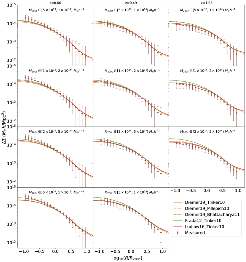
Figure 2: The measured $\Delta\Sigma$ profiles using downsampled particles for every 10 particles and theoretical $\Delta\Sigma$ as computed from the NFW profile using different concentration-mass relations (LHS in legend) in the one-halo regime and different halo-bias models (RHS in legend) in the two halo regimes, with errors taken to be $1-\sigma$ standard deviations; the measurements are consistent with theoretical predictions and the size of the errors is too large to distinguish between models. The same conclusion (not shown) holds for $\Delta\Sigma$ binned by $R_{\rm vir}$.

3.2 Measurements of $N_{\rm gal}$

3.2.1 Dataset for $N_{\rm gal}$ — SAGE galaxy catalog

The Semi-Analytic GALAXY Evolution (SAGE) is a catalogue of galaxies within MDPL2, generated through a post-processing step that places galaxies onto N-body simulations. This approach, known as a semi-analytic model (SAM), is computationally efficient compared to hydrodynamical simulations with fully self-consistent baryonic physics. SAMs reduce the computational time required by two to three orders of magnitude, allowing us to populate the entire 1 (Gpc/h)³ simulation volume with galaxies. SAGE’s statistical power enables us to conduct stacked weak lensing analyses.

The baryonic prescription of SAGE is based on the work of Croton et al. (2016), which includes updated physics in baryonic transfer processes such as gas infall, cooling, heating, and reionization. It also includes an intra-cluster star component for central galaxies and addresses the orphan galaxy problem by adding the stellar mass of disrupted satellite galaxies as intra-"cluster" mass. SAGE’s primary data constraint is the stellar mass function at $z=0$. Secondary constraints include the star formation rate density history (Somerville et al., 2001), the Baryonic Tully-Fisher relation (Stark et al., 2009), the mass metallicity relation of galaxies (Tremonti et al., 2004), and the black hole–bulge mass relation (Stark et al., 2009).

3.2.2 Model for $N_{\rm gal}$

To determine the number of galaxies inside a cluster-sized halo, we utilise the SAGE semi-analytic model and compute the total number of galaxies within a 3D radius around the halo centre. We compare the true richness ($N_{\rm gal}$) to $M_{\rm 200c}$ scaling relations between different models and the observed richness-mass relations from Costanzi et al. (2021) using data from the Dark Energy Survey (DES) Year-1 catalogue and mass-observable-relation from the South Pole Telescope (SPT) cluster catalogue (see Figure 3). The observed richness-mass relation is fitted as a log-linear model with $2-\sigma$ error bars that trace the posterior of the best-fit richness-mass model parameters. The $M_{\rm 500c}$ mass definition in the catalogue is converted to $M_{\rm 200c}$ using an NFW profile for the surface density of the cluster and adopting the Diemer & Joyce (2019) concentration-mass relation anchored at $z=0.35$, which is roughly the median redshift of the cluster sample.

We use the KLLR method to determine the local linear fit for our $N_{\rm gal}$-mass model, which relaxes the assumption of global log-linearity (Anbajagane et al., 2020). Realistic cluster finders, such as redMaPPer (Rykoff et al., 2014a), impose a colour-magnitude cut or a stellar mass cut, which are highly dependent on the red-sequence model or the spectral energy density model. We found that imposing a stellar mass cut of $10.5\log(M/M_{\odot})$ would correspond roughly to the bottom 5% percentile of SDSS detected galaxies (Maraston et al., 2013). However, this drastically decreases the number of galaxies in a halo, with most having $N_{\rm gal}$ in the single digits. As we are interested in the intrinsic covariance from the physical properties of the halo, we do not impose additional magnitude or stellar mass cuts. We confirm that, as described in Croton et al. (2016), the galaxy stellar mass distribution at $z=0$ is consistent with the best-fit double Schechter function calibrated with low-redshift galaxies from the Galaxy and Mass Assembly (GAMA) (Baldry et al., 2012) down to stellar masses of $\mathcal{M}<10^{8.5}M_{\odot}$.

Figure 3: Using different prescriptions of the richness count, we compare with the SPT-DES data (Costanzi et al., 2021). The richness estimator, with no stellar or color-magnitude cut, shows a similar trend with the data. In §4, we show that the results are robust to changes in the definition of the number count estimator.

Figure 3 illustrates that our $N_{\rm gal}$-mass models, which count the number of galaxies within a physical 3D radius and impose no colour-magnitude cut as redMaPPer does, resemble the observed richness-mass relations in terms of both slope and intercept when compared. However, we acknowledge that redMaPPer may suffer from projection effects that artificially inflate the number count of red-sequence galaxies within its aperture because of line-of-sight structures. Additionally, the $N_{\rm gal}$ count within the $R_{\rm vir}$ radius exceeds that of $R_{\rm 200c}$ as $R_{\rm vir}$ is greater than $R_{\rm 200c}$. In the toy model scenario, where we use a constant $1$ Mpc $h^{-1}$ radius, the slope of the mass-richness relation starts to decrease as the mass increases due to the increasing physical size of the clusters, as expected. The diversity of cluster radii and the resulting variation in the local slope and intercept of the $N_{\rm gal}$-mass relations demonstrate the robustness of our covariance model. In Section 4, we show that different radii/mass definitions have little impact on the parameters of our covariance model, thus establishing its independence from different reference radii, the definitions of cluster edges, and the resulting richness-mass relations.

4 Results: Covariance Shape and Evolution

In this section, we report the measurements for our covariance. In Figure 4, we find an anti-correlation between $N_{\rm gal}$ and $\Delta\Sigma$ at small scales across most redshift and mass bins spanned by our dataset, which we fit with the best-fit “Sigmoid” functional form of the expression

$$\rm{Cov}(\tilde{x})=s\Big{(}{\rm erf}(\frac{\sqrt{\pi}}{2}\tilde{x})+g\Big{)},$$ (28)

with $x\equiv\log{R/R_{\rm 200c}}$ the log-radius and $\tilde{x}\equiv(x-\gamma)/\tau$ the scaled and offset log-radius. In Appendix A, we offer statistical verification of the best-fit functional form.

We first describe the evolution of the covariance in §4.1 by binning across the $(M,z)$ bins. Next, in §4.2, we present an alternative binning scheme based on halo peak height that can provide insight into the dependence of the time formation history of the covariance scale.

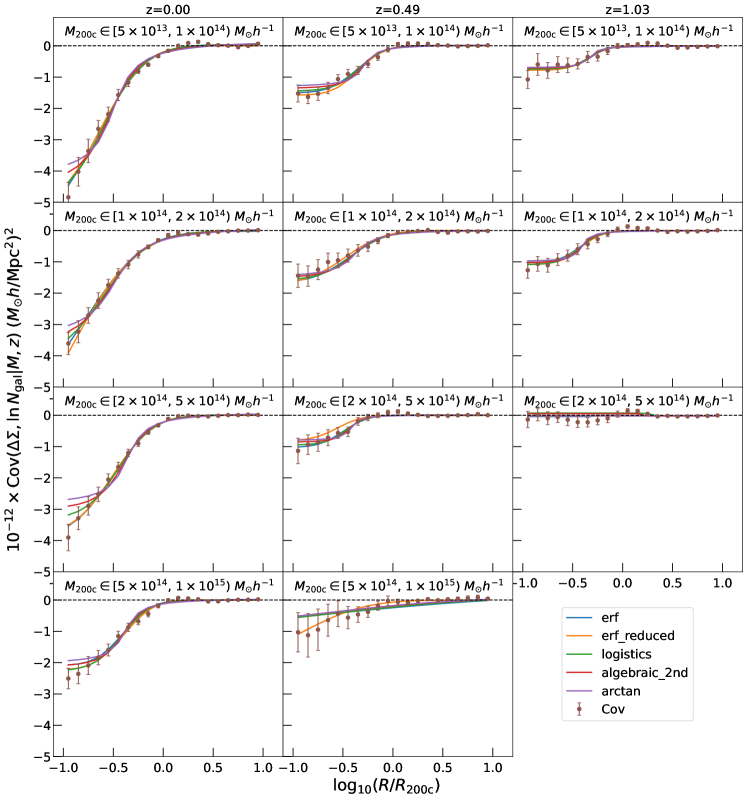
Figure 4: Comparison of Cov($\Delta\Sigma$, $N_{\rm gal}$) and different functional forms using the full model. The functions are classes of "Sigmoid" functions. In all bins, the error function outperforms other functional forms in their DIC parameters, providing good $\chi^{2}$ values. For $M_{\rm 200c}\in[5\times 10^{14},1\times 10^{15})$ at $z=0.49$ and $M_{\rm 200c}\in[2\times 10^{14},5\times 10^{15})$ at $z=1.03$, the posteriors of the full models do not converge as the size of the covariance is too small.

4.1 Binned in $(M,z)$

Our best-fit parameters in Table 6 indicate that in 9 out of 12 $(M,z)$ bins, the Cov($\Delta\Sigma,\ln N_{\rm gal}\mid M,z)$ rejects the null-correlation hypothesis with high statistical significance ($p-{\rm value}<0.01$). However, in two bins, specifically $M_{\rm 200c}\in[5\times 10^{14},1\times 10^{15})\ M_{\odot}h^{-1}$ at $z=0.49$ and $M_{\rm 200c}\in[2\times 10^{14},5\times 10^{15})\ M_{\odot}h^{-1}$ at $z=1.03$, the magnitude of the covariance is relatively small compared to the size of their errors. Consequently, it becomes challenging to constrain the shape parameters in these two bins, and the covariance is consistent with the null hypothesis. Furthermore, we exclude the bin $M_{\rm 200c}\in[5\times 10^{14},1\times 10^{15})\ M_{\odot}h^{-1}$, $z=1.03$ due to the limited number of halos it contains.

Our results suggest that the shape of the covariances can be accurately described by the full error function. This is evident from the right tail $p$-value for $\chi^{2}$, which exceeds the statistical significance level of $0.05$ for all bins except one with constrained shape posteriors. Additionally, for $R\geq R_{\rm vir}$ or $R\geq R_{\rm 200c}$, the covariance aligns with the null-correlation hypothesis. This alignment is reflected in the fact that all 9 bins with constrained posterior shape have best-fit $g$ values within $2\sigma$ of $g=-1$. Deviations from $g=-1$ can be interpreted as evidence of disagreements with the Press-Schechter formalism (Press & Schechter, 1974) of spherical collapse halos, which can be originated from the presence of anisotropic or non-Gaussian matter distribution around halos at large scales (Lokken et al., 2022), or it can be an indicator of an open-shell model of halos that allows for the bulk transfer of baryonic and dark matter in and out of the halo potential well during the non-linear collapse.

With $g=-1$ fixed, the reduced error function marginally improves the constraints in most bins. However, with the reduced model, we can provide posterior constraints for $M_{\rm 200c}\in[5\times 10^{14},1\times 10^{15})M_{\odot}h^{-1}$ at $z=0.49$ and $M_{\rm 200c}\in[2\times 10^{14},5\times 10^{15})M_{\odot}h^{-1}$ at $z=1.03$, which the full model failed to constrain but with very loose posterior constraints. The estimated parameters for both the full and reduced models are presented in Table 6 and Table 7, respectively.

To assess the impact of varying the definition of the halo radius on our measurements of the shape of the covariance, we considered two factors: the scale dependence of $\Delta\Sigma$ discussed in §2.1.3 and §3.1, and the alteration of the richness-mass relation as shown in Figure 3 in §3.2. Figure 5 demonstrates that there is no apparent evolution of the shape parameters $\boldsymbol{\theta}\in\{\tau,\gamma,g\}$ when altering the scale dependence for $\Delta\Sigma$ or the true richness count. However, we find marginal $3\sigma$ evidence of a difference in the vertical scale of the covariance $s$ when changing the scale normalisation from $r_{p}=R/R_{\rm 200c}$ to $r_{p}=R/R_{\rm vir}$ while using the same true richness count. As halos exhibit more self-similarity in the inner regions when scaled by $R_{\rm 200c}$ (Diemer & Kravtsov, 2014), we adopt this as our radius normalisation and use the number of galaxies enclosed within $R_{\rm 200c}$ as our true richness count.

Subsequently, we explored the evolution of the shape parameters with respect to $(M,z)$ and found no strong mass dependence. However, we observed a monotonically decreasing redshift dependence of the vertical scale parameter $s$, as illustrated in Figure 6. To explain both the halo mass and the redshift dependence, we used the peak height of the halo, $\nu(M,z)$.

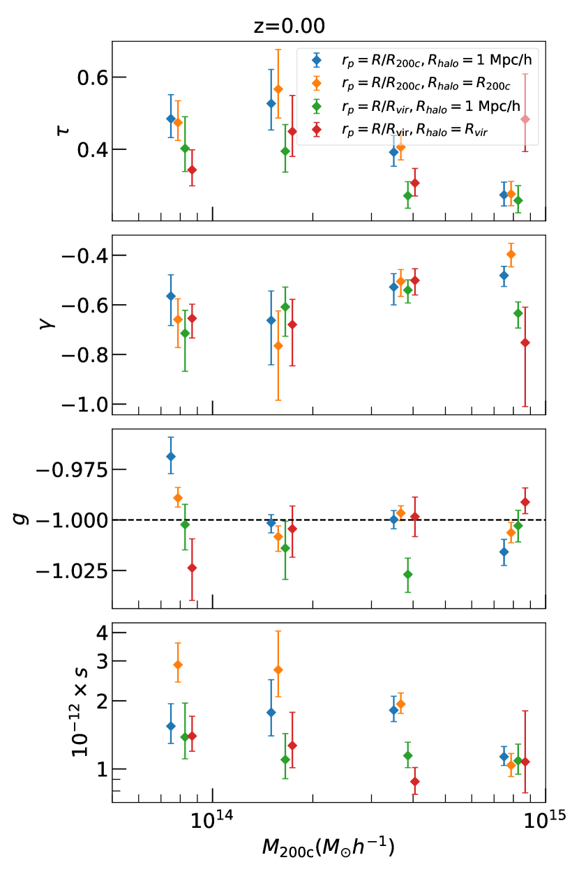
Figure 5: Evolution of Cov($\Delta\Sigma$, $N_{\rm gal}\mid M,z$) shape parameters with respect to mass and radial binning schemes and $N_{\rm gal}$ definition at fixed redshift at z=0. $\Delta\Sigma$ is binned in equal log-space radial bins in $R/R_{\rm 200c}$ or $R/R_{\rm vir}$; for each radial binning, the number count of galaxies inside the cluster is given by a constant radius of $1\ {\rm Mpc}h^{-1}$ or $R_{\rm 200c}$ when binned by $R_{\rm 200c}$ and $R_{\rm vir}$ when binned by $R_{\rm vir}$. We find no strong evolution in the shape or scale of the covariance under different binning schemes or $N_{\rm gal}$ definitions. The trend is consistent across different redshift bins and demonstrates the robustness of the covariance under different true richness definitions.

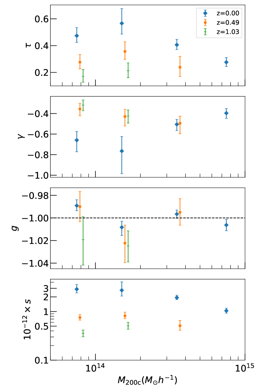
Figure 6: Evolution of Cov($\Delta\Sigma$, $N_{\rm gal}\mid M,z$) shape parameters of the error function with respect to mass and redshift, binned in units of $R_{\rm 200c}$ and with $N_{\rm gal}$ taken to be the number of clusters inside the $R_{\rm 200c}$ radius of the cluster. There is no strong dependence of $\tau$, $\gamma$, and $g$ with respect to mass and redshift and a strong monotonically decreasing $s$ with respect to redshift. At $M_{\rm 200c}\in[5\times 10^{14},1\times 10^{15})$, $z=0.49$ and $M_{\rm 200c}\in[2\times 10^{14},5\times 10^{15})$, $z=1.03$ the covariance is consistent with null at $p=0.01$ and $p=0.05$ levels, respectively.

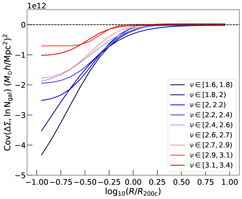
Figure 7: Best-fit “full” error function model for ${\rm Cov}(\Delta\Sigma,\ln N_{\rm gal}\mid M,z)$ when binned in deciles of halo peak height. The first nine bins reject the null hypothesis at a $p<0.01$ level, and the highest decile rejects the null hypothesis at a $p<0.05$ level. We can provide posterior constraints for all bins in peak height except for the one with the highest peak height value.

4.2 Binned by peak height

An alternative binning scheme that encapsulates both the halo mass and redshift information is to bin halos by the peak height parameter, defined as

$$\nu=\frac{\delta_{c}}{\sigma(R,a)},$$ (29)

where $\delta_{c}(z)$ is the collapse overdensity at which gravitational collapses enter the non-linear regime and $\sigma(R,a)$ is the smoothing scale seen in Equation (36) at the radius of the cluster. For an Einstein-de Sitter universe ($\Omega_{m}=1$, $\Omega_{\Lambda}$ = 0) $\delta_{c}\approx 1.686$ at the epoch of collapse and is weakly dependent on cosmology and redshift (Percival, 2005). $\sigma(R,a)$ scales as $\sigma(M,a)=\sigma(M,a=1)D_{+0}(a)$ at the linear collapse regime, where $D_{+0}(a)\equiv D_{+}(a)/D_{+}(a=1)$. Here $D_{+}(a)$ is the linear growth factor defined as

$$D_{+}(a)=\frac{5\Omega_{M}}{2}E(a)\int^{a}_{0}\frac{da^{\prime}}{[a^{\prime}E(a^{\prime})]^{3}},$$ (30)

for a $\Lambda$CDM cosmology, where $E(a)\equiv H(a)/H_{0}$ is the normalised Hubble parameter. $\sigma(R,z)$ depends strongly on redshift, and hence, the peak height $\nu$ strongly depends on the halo radius and the redshift of non-linear collapse.

The peak height has been adopted to simplify the mass and redshift dependence in various halo properties, such as halo concentration (Prada et al., 2012) and halo triaxiality (Allgood et al., 2006). Here, we explore whether the peak height can serve as a universal parameter to explain the scale and shape of ${\rm Cov}(\Delta\Sigma,\ln N_{\rm gal}\mid M,z)$. We bin the halos into deciles of $\nu$ and set posterior constraints on the shape of the covariance using our erf model in the full model case. In the highest decile (90%-100% percentile), we reject the null-correlation hypothesis at the $p=0.01$ level, but due to the size of the error bars, the shape of the parameters $\tau$, $\gamma$, and $g$ and largely unconstrained and $s=10^{12}\times 0.16^{+0.34}_{-0.12}$. Due to the large degeneracy, we exclude the highest decile from our dataset and limit the range of our model to $\nu\in[1.57,3.40)$, which spans 0% to 90% of our sample set. The large error bars may be due to the fact that the halo abundance as a function of $\nu$ falls precipitously around $\nu\sim 4$, so the highest decile spans a wide tail of high $\nu\in[3.4,4.6)$. The plots in Figure 7 are the best-fit templates when binned by peak height, and Figure 8 shows the best-fit parameters and peak height dependence as a function of peak height. We do not see a strong dependence on the peak height for $\tau$, $\gamma$ and $g$. For $s$, its dependence on $\nu$ can be modelled as a log-linear relation of the form

$$\log_{10}(s)=C_{s}+\alpha\nu,$$ (31)

with $C_{s}=13.07^{+0.26}_{-0.26}$ and $\alpha=-0.44^{+0.11}_{-0.11}$. At the highest decile, the $s=10^{12}\times 0.16^{+0.34}_{-0.12}$ falls within the $1\sigma$ confidence band of the log-linear fit. Compared to the first 9 deciles, the fit yields a $\chi^{2}$ $p$-value of 0.73. The negative slope between $s$ and $\nu$ indicates that more massive halos at the cosmic era of their formation exhibit a lesser anti-correlation between $\Delta\Sigma$ and $\ln N_{\rm gal}$.

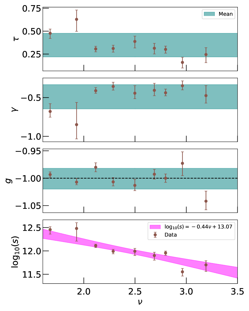
Figure 8: The evolution of shape parameters for ${\rm Cov}(\Delta\Sigma,\ln N_{\rm gal}\mid M,z)$ binned in deciles of the peak height $\nu$, excluding the highest decile. The parameters $\tau$, $\gamma$, and $g$ show little dependency with $\nu$ while the vertical scale $s$ exhibits a log-linear relationship with $\nu$ of the form shown in Equation (31). The mean $g$ is consistent with -1. The horizontal teal bands fill the $1\sigma$ range around the mean, and the pink line is the best log-linear fit between $s$ and $\nu$ with $1\sigma$ confidence bands.

5 Impact of ${\rm Cov}(\Delta\Sigma,\ln N_{\rm gal}\mid M,z)$ on weak lensing measurements

Figure 9: The percent level change in stacked $\Delta\Sigma$ measurements after including the covariance terms in Equations (19) and (20). The slope and curvature of the halo mass function are calculated numerically from the Tinker et al. (2008) halo mass function in our nominal correction. The errors are taken from bootstrapped errors of the covariance. We compare the results with first-order corrections from other halo mass functions using Watson et al. (2013); Bocquet et al. (2016); Despali et al. (2016). We find that the percentile difference in $\Delta\Sigma$ owns the choice of halo mass functions, and the first and second order corrections are subdominant to the first order correction itself, which is at a $\sim 1\%$ level at small scales for $\Delta\Sigma$ and propagates into an upward correction of stacked halo mass of $\delta M/M\sim 2-3\%$ for most bins after applying the correction.

To assess the impact of ${\rm Cov}(\Delta\Sigma,\ln N_{\rm gal}\mid M,z)$ on the scaling relation $\langle\Delta\Sigma\mid N_{\rm gal},z\rangle$, we utilise Equation (19) for the first-order correction and Equation (20) for the 2nd order. The mean mass of the halos in each $(M,z)$ bin is chosen as the pivot mass, and the intercept $\pi_{N_{\rm gal}}$ and slope $\alpha_{N_{\rm gal}}$ for the richness-mass scaling relation shown in Equation (11) are computed locally at the pivot point in each bin $(M,z)$ bin. Our mock data, binned in $R_{\rm 200c}$, yields results that are consistent with the global richness-mass relation found in the literature (Bocquet et al., 2016; Costanzi et al., 2021; To et al., 2021), as shown in Figure 3.

For the correction terms, we adopt the Tinker et al. (2008) halo mass function as our nominal model and compute the numeric log-derivative for values of $\gamma_{1}$ and $\gamma_{2}$, the log-slope and curvature of the halo mass function around the pivot mass. We compare the Tinker mass function results with others, including Watson et al. (2013); Bocquet et al. (2016); Despali et al. (2016), and find that the difference is subdominant to the first-order correction, which is at a $\sim 1\%$ level at small scales, as shown in Figure 9.

To estimate the mass bias, we use the same modelling approach for individual halos to propagate the stacked $\langle\Delta\Sigma\mid N_{\rm gal}\rangle$ signal. Specifically, we assume an NFW profile using the concentration-mass model of Diemer & Joyce (2019) in the one-halo regime. We convert the 3D overdensity of the modelled halo $\xi_{hm}$ to $\Delta\Sigma$ using Equations (2) and (5), and then apply the first-order correction in Equation (19). Using a Monte Carlo method, we estimate the expected mass after this correction and report the change in the halo mass with this correction for each $(M,z)$ bin. As shown in Figure 9, we find that adding the correction leads to an upward correction of the stacked halo mass of approximately $\delta M/M\sim 2-3\%$ for most $(M,z)$ bins.

6 Explaining the covariance

6.1 Secondary Halo Parameter Dependence of $\ln N_{\rm gal}$

We employed a multi-variable linear regression model to determine the best-fit when incorporating secondary properties in the regression. Initially, considering the full set of parameters listed in Table 3, we applied a backward modelling scheme to identify the relevant parameters of interest. Details of this process can be found in Appendix D, which led to the selection of the following secondary halo parameters for our model: $\Pi\subset\{\Gamma_{\rm 2dyn},a_{\rm 1/2},c_{\rm vir},T/|U|,X_{\rm off}\}$. The resulting model demonstrated good explanatory power, as indicated by a high $R^{2}$ coefficient. Additionally, the model passed various tests, including variance inflation, global F-statistic, partial F-statistic, T-statistic, scatter heteroscedasticity, and scatter normality in most cases. Specifically, through a comparison of $F_{\rm partial}$ values, we found that richness could be modelled by a multi-linear equation involving all secondary halo parameters. Further information can be found in Table 8, where the F-statistic demonstrates that all parameters are statistically significant. Only when considered collectively can they accurately reflect the dependence of richness on halo formation history.

To establish informative priors for upcoming weak lensing surveys such as HSC and LSST, we examined whether the dependence of $N_{\rm gal}$ on secondary halo properties, as inferred from the slope $\beta_{N_{\rm gal}}$, aligns with arguments based on halo formation physics. We expected that $\beta_{{N_{\rm gal},c_{\rm vir}}}$ resulting from the formation of satellite galaxies (equivalent to $N_{\rm gal}-1$ in the presence of a central galaxy) within halos would exhibit a negative relation, i.e., $\beta_{{N_{\rm gal},c_{\rm vir}}}<0$. Simulation-based studies have suggested that early-forming halos possess higher concentrations (Wechsler et al., 2002), and correspondingly, high-concentration halos (which form early) have fewer satellite galaxies due to galaxy mergers within the halos (Zentner et al., 2005). This effect is known as galaxy assembly bias (Wechsler & Tinker, 2018) — the change in galaxy properties inside a halo at fixed mass due to the halo formation history. There is marginal evidence of the existence of assembly bias from recent observations using galaxy clustering techniques (Zentner et al., 2019; Wang et al., 2022), as well as measurements of the magnitude gap between the brightest central galaxy (BCG) and a neighbouring galaxy as a proxy for formation time (Hearin et al., 2013; Golden-Marx & Miller, 2018; Farahi et al., 2020).

As noted in Table 8, the signs of $\beta_{N_{\rm gal},i}$ for $i\in\{a_{1/2},c_{\rm vir},T/|U|,\Gamma_{\rm 2dyn},X_{\rm off}\}$ align with our expectations of assembly bias in most bins. However, the sign of $\beta_{{N_{\rm gal},c_{\rm vir}}}$ changes from negative ($<0$) at low redshifts to positive ($>0$) in some mass bins at medium and high redshifts. On the contrary, we observe a diminishing impact of secondary halo properties on richness (indicated by a smaller absolute value for $\beta_{N_{\rm gal},c_{\rm vir}}$), the reversal of the coefficient’s sign cannot be solely attributed to statistical fluctuations around zero, as some values are inconsistent with zero at levels exceeding $3\sigma$.

This issue can be attributed to the effect of major mergers on concentration. Recent studies (Ludlow et al., 2012; Wang et al., 2022; Lee et al., 2023) have shown that halos, during major merger events, experience a transient fluctuation in concentration before returning to the mean relation over a time period slightly less than the dynamical time of the halo. The measured concentration spike during major mergers, particularly prominent at higher redshifts, could explain a positive $\beta_{\{N_{\rm gal},c_{\rm vir}\}}$.

To test this hypothesis, we employ a toy model that divides halos in each $(M,z)$ bin based on the median $\Gamma_{\rm 1dyn}$ into low-$\Gamma_{\rm 1dyn}$ and high-$\Gamma_{\rm 1dyn}$ subsamples. Figure 10 displays the halo concentration plotted against the richness residuals, separated by $\Gamma_{\rm 1dyn}$, at three benchmark bins of $M_{\rm 200c}\in[5\times 10^{13},1\times 10^{14})\ M_{\odot}h^{-1}$ and three different redshift snapshots of $z=0,0.49,1.03$. At $z=0$, we observe a negative slope as expected from halo formation physics for both low-$\Gamma_{\rm 1dyn}$ and high-$\Gamma_{\rm 1dyn}$ subsamples, as well as for the overall sample. Furthermore, we observe a change in the slope between the low-$\Gamma_{\rm 1dyn}$ and high-$\Gamma_{\rm 1dyn}$ sub-samples, which can be explained by the gradual increase (or decrease) in concentration ($\Gamma_{\rm 1dyn}$) over time, even without major merger events (Wechsler et al., 2002; Zhao et al., 2003; Lu et al., 2006). At redshifts of $z=0.49,1.03$, we observe a positive slope in the overall and/or high-$\Gamma_{\rm 1dyn}$ samples, which contradicts the scaling relations between HOD and concentration in models that track their gradual evolution over $T\gg T_{\rm 1dyn}$. However, in the presence of major mergers, when $\Gamma_{\rm 1dyn}$ is significantly enhanced, the halo concentration may also experience a transient spike after the merger. The deviation from hydrostatic equilibrium provides a plausible explanation for a positive $\beta{\{N_{\rm gal},c_{\rm vir}\}}$, which could be fully tested on MDPL2 through the reconstruction of halo merger trees, an analysis beyond the scope of this paper.

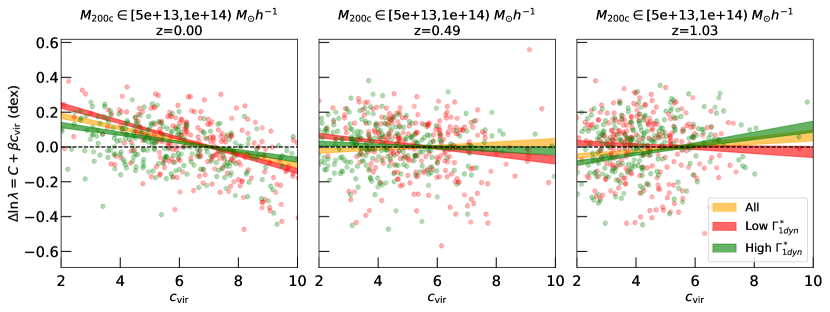
Figure 10: Residual log-richness versus concentration relation in subsets of halo mass accretion rate (MAR). The figure consists of three panels, left, middle, and right, corresponding to $z=0$, $z=0.49$, and $z=1.03$, respectively, each focuses on a benchmark mass bin of $M_{\rm 200c}\in[5\times 10^{13},1\times 10^{14})M_{\odot}h^{-1}$. The sample is split into low and high $\Gamma_{\rm 1dyn}$ based on their median values. The scatter plot illustrates the data points, while the shaded regions show the best-fit linear fit with $1\sigma$ confidence interval for the main sample and each sub-sample. At $z=0$, the richness-concentration relation exhibits a negative slope, consistent with our expectations of halo formation physics. The slopes for the low and high $\Gamma_{\rm 1dyn}$ subsamples diverge due to the negative correlation between concentration and MAR. However, at $z=0.49$ and $z=1.03$, the slopes for the entire sample and/or the high $\Gamma_{\rm 1dyn}$ subsample become positive, contrary to our observations of the richness-concentration relation. In contrast, the low $\Gamma_{\rm 1dyn}$ subsample still shows a negative slope. These findings suggest that at medium to high redshifts, a subset of unrelaxed and recently merged halos with high MAR could elevate the concentration from its expected value at hydrostatic equilibrium.

6.2 Secondary Halo Parameter Dependence of $\Delta\Sigma$

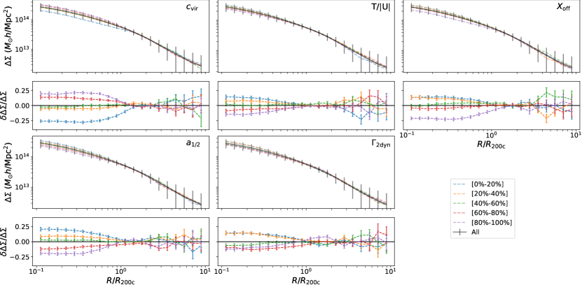
Figure 11: The dependence of $\Delta\Sigma$ on accretion history parameters in $M_{\rm 200c}\in[2\times 10^{14},5\times 10^{14})M_{\odot}h^{-2}$, $z=0$. In each of the 5 panels is plotted the $\Delta\Sigma$ in different quintiles of the accretion history parameter $\Pi\in\{a_{1/2},c_{\rm vir},T/|U|,\Gamma_{\rm 2dyn},X_{\rm off}\}$ compared to the mean $\Delta\Sigma$. For $\{a_{1/2},T/|U|,\Gamma_{\rm 2dyn},X_{\rm off}\}$ there is a strong negative correlation at small scales at $R\lesssim R_{\rm 200c}$ and for $c_{\rm vir}$ we find a strong positive correlation at $R\lesssim R_{\rm 200c}$. Comparing the width of $\Delta\Sigma$ binned at different quintiles of $\Pi$ with the standard deviation of the profiles, we find that accretion history parameters account for much of the variance at small scales and play a negligible role at large scales.

In this section, we employ a multi-linear regression approach to model the richness, similar to the methodology described in §6.1. We extend this approach to the model $P(\Delta\Sigma|N_{\rm gal}(\Pi),M,z)$ as a linear function of $\Pi$. Upon analysing different $(M,z,r_{p})$ bins, we observe that the reduced parameters $\Pi\subset\{a_{1/2},c_{\rm vir},T/U,\Gamma_{\rm 2dyn},X_{\rm off}\}$ pass the VIF test for multi-collinearity. This indicates that $\ln N_{\rm gal}$ can be described without redundancy by a linear decomposition of these reduced parameters. Furthermore, most bins exhibit homoscedasticity, as confirmed by passing the Breusch-Pagan Lagrange Multiplier test. This implies that the scatter terms $\sigma_{\Delta\Sigma}$ and $\sigma_{\Pi_{i}}$ remain constant within each bin, with a few exceptions. Lastly, the scatter $\sigma_{\Delta\Sigma|N_{\rm gal}}$ in most bins (with a few exceptions) meets the criteria of the Shapiro-Wilk test for Gaussianity, suggesting that the distribution closely resembles a Gaussian distribution.

Assuming that $P(\ln N_{\rm gal}|M,z)$ and $P(\Delta\Sigma|M,z)$ can be modelled with a normal distribution (e.g., Anbajagane et al., 2020; Costanzi et al., 2021; To et al., 2021), then $P(\Delta\Sigma\mid N_{\rm gal},\Pi,M,z)$ is another normal distribution with mean

$$\langle\Delta\Sigma|N_{\rm gal},\Pi,M,z\rangle~{}= ~{}\langle\Delta\Sigma|N_{\rm gal},M,z\rangle$$ (32)

$$+ C_{1}\sigma_{\Delta\Sigma}\Big{(}\sum_{i}\frac{\beta_{N_{\rm gal},i}}{\sigma_{\Pi_{i}}}\rho_{\Delta\Sigma-\Pi_{i}}\times(\Pi_{i}-\langle\Pi_{i}|M,z\rangle)\Big{)}$$

and variance

$$\qquad\sigma^{2}_{\Delta\Sigma|\ln{N_{\rm gal}}}\quad= ~{}\sigma^{2}_{0}+C_{2}\sum_{i}{\beta_{N_{\rm gal},i}^{2}\sigma^{2}_{\Pi_{i}}(1-\rho^{2}_{\Delta\Sigma-\Pi_{i}})}+$$ (33)

$$C_{3}\sum^{j\neq i}_{i,j}{\rho_{\Pi_{i}-\Pi_{j}}\sigma_{\Pi_{i}}\sigma_{\Pi_{j}}}.$$

Parameters $C1$, $C2$, $C3$, and $\sigma_{0}$ can be explicitly derived where $P(\ln N_{\rm gal}|M,z)$ and $P(\Delta\Sigma|M,z)$ are known by the exercise of completing the squares inside the exponents, but the exact values are not essential for this paper.

We note that only in bins of $R\lesssim R_{\rm 200c}$ do the multilinear regression models pass the global F-statistic test and the T-statistic test for each parameter. This result suggests that at $R\gtrsim R_{\rm 200c}$, we find little correlation between $\Delta\Sigma$ and $\Pi_{i}$. Because the scatter still passes the Shapiro-Walk test for Gaussanity, the conditional probability $P(\Delta\Sigma|N_{\rm gal},M,z)$ at large scales is still normally distributed, but with $\rho_{\Delta\Sigma-\Pi_{i}}=0$. By setting $\rho_{\Delta\Sigma-\Pi_{i}}=0$ the variance can be reduced to

$$\sigma^{2}_{\Delta\Sigma|N_{\rm gal}}\quad=\sigma^{2}_{0}+\sum_{i}{\beta_{N_{\rm gal},i}^{2}\sigma^{2}_{\Pi_{i}}}+\sum^{j\neq i}_{i,j}{\rho_{\Pi_{i}-\Pi_{j}}\sigma_{\Pi_{i}}\sigma_{\Pi_{j}}}.$$ (34)

We visualise the dependence of $\rho_{\Delta\Sigma-\Pi_{i}}$ on $R/R_{\rm 200c}$ in Figure 11. By binning $\Delta\Sigma$ in quintiles of $\Pi_{i}$ we find a strong correlation for all parameters at $R\lesssim R_{\rm 200c}$ and a null correlation at $R\gtrsim R_{\rm 200c}$. On small scales, our results show a positive correlation for concentration and a negative correlation for $\{a_{1/2},T/U,\Gamma_{\rm 2dyn},X_{\rm off}\}$. We observe that this trend holds for all $(M,z)$ bins plotted for a benchmark bin of $M_{\rm 200c}\in[2\times 10^{14},5\times 10^{14})M_{\odot}h^{-1}$ at $z=0$.

The dependence of $\Delta\Sigma$ on secondary halo parameters qualitatively agrees with Xhakaj et al. (2022) wherein they targeted a narrow mass bin, with residual mass dependency inside the bin resampled so that mass follows the same distribution. In our work, we remove the mass dependency with the KLLR method (Farahi et al., 2022a), which achieves the same effect. We extend their results to mass and redshift bins probed by the optical surveys and quantitatively show that the dependence of $\Delta\Sigma$ on $\Pi$ can be modelled as a multi-linear equation.

6.3 Results: Secondary Halo Parameter Dependence of ${\rm Cov}(\Delta\Sigma,\ln{N_{\rm gal}}\mid M,z)$

In Figure 12, we observe that the total covariance ${\rm Cov}(\Delta\Sigma,\ln N_{\rm gal}|M,z)$, which remains after removing the contribution of each secondary halo parameter $\beta_{N_{\rm gal},i}{\rm Cov}(\Delta\Sigma,\Pi_{i}|M,z)$, is consistent with zero at a significance threshold of $0.05$ in all bins. The errors on the total covariance and individual contributions are computed using bootstrapping, and the errors on the remaining term are determined by adding the errors of the total and individual terms in quadrature.

Based on our hypothesis in Equation (27), we conclude that the set of secondary halo parameters $\Pi$, which are related to the formation time and the mass accretion history of the halos, can fully explain the joint distribution of $\Delta\Sigma$ and $\ln N_{\rm gal}$ given the precision allowed by current errors, limited by the resolution limit (see Appendix B for information on particle resolution and measurement errors).

Since the joint distribution of $\Delta\Sigma$ and $\ln N_{\rm gal}$ follows a multivariate normal distribution, $P(\Delta\Sigma,\ln N_{\rm gal}|M,z)$ is completely characterised by its mean relation and ${\rm Cov}(\Delta\Sigma,\ln N_{\rm gal}\mid M,z)$. It should be noted that the contribution of each individual parameter to the total covariance, $\beta_{N_{\rm gal},i}{\rm Cov}(\Delta\Sigma,\Pi_{i}\mid M,z)$, is determined by the richness dependency captured by the slope $\beta_{N_{\rm gal},i}$ and the $\Delta\Sigma$ dependency represented by ${\rm Cov}(\Delta\Sigma,\Pi_{i}\mid M,z)$. Qualitatively, individual contributions to total covariance maintain their sign when both $\Delta\Sigma$ and $N_{\rm gal}$ contributions preserve their sign. Consistent with the arguments of halo formation, $\Pi$ correlates with $\Delta\Sigma$ at small scales, as demonstrated in Figure 11 across all $(M,z)$ bins. In most cases, the dependence of the richness on secondary halo parameters also maintains its sign across the $(M,z)$ bins. In instances where we encounter a sign reversal in the $\ln N_{\rm gal}-c_{\rm vir}$ relation, we speculate that it is due to a transient increase in concentration following a major merger.

Furthermore, the total and individual contributions to the covariance tend to decrease in magnitude at smaller scales with increasing redshift. This decrease in covariance can be attributed to two factors: the decreasing explanatory power of $\Pi$ on richness, as indicated by the decreasing values of $R^{2}$ and $F_{\rm partial}$ values in Table 8, and the decreasing absolute value of ${\rm Cov}(\Delta\Sigma,\Pi_{i}\mid M,z)$. This trend aligns with the idea that as halos have more time to form, the secondary halo properties related to the mass accretion history become more significant both in richness and in $\Delta\Sigma$. As discussed in §4, the dependence of the mass and redshift on covariance can be explained by the halo peak height, $\nu(M,z)$.

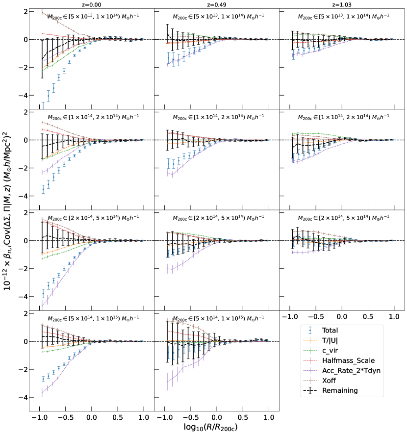
Figure 12: The dependence of ${\rm Cov}(\Delta\Sigma,\ln N_{\rm gal})$ on secondary halo parameters $\Pi$. The solid blue line is the total covariance. The dashed lines of the lines represent the covariance contribution coming from each of the secondary halo parameters modelled and governed by Equation 27, where ${\rm Cov}(\Delta\Sigma,\Pi|M,z)$ comes from the dependence of $\Delta\Sigma$ and the slope $\beta_{i}$ is the dependency of richness. The thick black dashed line is the remaining covariance after removing the contribution from each $\Pi_{i}$ term; the errors are obtained by adding the total and individual errors in quadrature without considering the correlations between terms. In agreement with our hypothesis in Equation 27, the remaining term is consistent with null at a $p<0.01$ level for all bins.

7 Discussions

Intrinsic vs. Extrinsic Covariance.

Our study distinguishes between the intrinsic covariance investigated here and that observed in empirical cluster data sets. This distinction arises from systematic biases introduced by the cluster finder algorithm (extrinsic component) and the underlying physics governing halo formation (intrinsic component). Specifically, our analysis involves counting galaxies in 3D physical space. In contrast, a realistic cluster finder like redMaPPer (Rykoff et al., 2014b) employs a probabilistic assignment of galaxies to halos in 2D physical space, considering projected radii and redshift through color matching onto the red sequence. Our study does not account for the observational systematics in redMaPPer associated with uncertainties in photometric redshifts and projection effects (Rozo et al., 2015; Farahi et al., 2016).

We find that the fractional amplitude of the bias and the scale dependence observed in our results are comparable to those reported by Farahi et al. (2022b), who measured the covariance between halo galaxy number count after applying a realistic stellar mass cut. The enclosed mass within a 3D radius using the IllustrisTNG100 simulation is anchored at $z=0.24$. By comparing our findings to those obtained using a realistic cluster finder such as redMaPPer, we can unravel intrinsic and extrinsic contributions to the covariance between weak lensing observables (Wu et al., 2022). This work provides more profound insights into the distinct effects originating from the underlying physics and the methodology employed in cluster-finding algorithms (Euclid Collaboration et al., 2019).

Projection Effects.

A noteworthy distinction arises regarding the covariance observed in our study compared to others examining projected space clusters. Projection effects can potentially introduce a sign flip in the covariance, as they can positively bias both $\Delta\Sigma$ and richness (Costanzi et al., 2019; Wu et al., 2022; Zhang & Annis, 2022). Wu et al. (2022) detected a positive correlation between $\Delta\Sigma$ and $\ln N_{\rm gal}$ employing Buzzard simulations, where $\Delta\Sigma$ were measured using dark matter particles and galaxy counts were performed within a cylindrical region of depth $60$ Mpc/h. Their investigation revealed that the positive correlation primarily stems from galaxy number counts beyond the halo’s virial radius and within $60$ Mpc/h. On the other hand, using the Dark Quest emulator and HOD-based galaxy catalogues (Nishimichi et al., 2019), Sunayama et al. (2020) found negligible deviations from the mean relation at small scales and an overall reduction in selection bias at large scales, approximately halving the effect observed by Wu et al. (2022). Furthermore, Huang et al. (2022), using data from the Subaru Hyper Suprime-Cam (HSC) survey, observed that the selection bias is most prominent in the vicinity of the transition from the one-halo to the two-halo regime, as evidenced by the comparison between the outer stellar mass proxy and richness. In a study based on the IllustrisTNG300 simulation, Zhang & Annis (2022) discovered a net positive correlation between the fitted weak lensing mass and the projected 2D number count of the halo when conditioned on the halo mass.

These results suggest that projection effects can potentially introduce a positively correlated bias to both $\Delta\Sigma$ and $N_{\rm gal}$. We can estimate the impact of projection effects by comparing the intrinsic covariance measured in our study with the total covariance observed in the projected space. Consequently, our results serve two essential purposes: (i) elucidating the physical origins of the negative covariance and (ii) discerning intrinsic and extrinsic components to determine the covariance attributable to projection effects accurately.

Radial Dependence.

There is a notable difference in the reported amplitude and scale dependence of covariance, which can be attributed to discrepancies in the employed halo occupation density models. Notably, a distinctive scale dependence discrepancy exists between simulation-based investigations of projection effects (Sunayama et al., 2020; Wu et al., 2022; Salcedo et al., 2020) and observational data from the HSC (Huang et al., 2022). In particular, the analysis of observational data reveals a prominent 1 Mpc bump, which could be explained by uncertainties inherent in observations, such as miscentering effects. It is crucial to gain insights into the sensitivity of the covariance with respect to the model parameters and the influence of selection effects. Understanding these factors is essential to comprehensively interpret and account for the observed covariance in galaxy cluster survey studies.

Accuracy vs. Precision.

The statistical power of current and future surveys enables us to determine the normalisation and slope of the mass–observable relations at a few percent levels (e.g., Farahi et al., 2016; Mantz et al., 2016b; Mulroy et al., 2019; To et al., 2021). However, these estimates are susceptible to known and unknown sources of systematic errors that inflate the uncertainties. These uncertainties introduce biases and degrade the accuracy of the results. Therefore, it is essential to carefully identify, quantify, and account for these systematic effects to ensure robust and reliable measurements. In this work, we focus on studying one of these sources of systematic uncertainty that was not considered previously.

8 Summary

This work reveals insights into the scale-dependent covariance between weak lensing observables and the physical properties of the halo. Using the MDPL2 N-body simulation with galaxies painted using the SAGE semi-analytic model, we present several key findings:

• We observe that the intrinsic covariance between $\Delta\Sigma$ and $\ln N_{\rm gal}$ enclosed within a 3D radius is negative at small scales and null at large scales in $(\ln M,z)$ ranges that cover optical surveys.

• We model the shape of the covariance across all bins using an error function that is insensitive to the radius definition used to define halo boundaries.

• We find that the magnitude of the covariance is relatively insensitive to mass and decreases considerably with increasing redshift. The $(M,z)$ dependence of the shape of the covariance can be encapsulated by the peak height parameter $\nu(M,z)$, which suggests that the scale of the covariance is related to the formation history of halos.

• We show that incorporating the covariance into $\langle\Delta\Sigma|N_{\rm gal},z,r_{p}\rangle$ using the first-order expansion of the halo mass function yields about $>1\%$ bias on $\langle\Delta\Sigma|N_{\rm gal},z,r_{p}\rangle$ at small scales, which implies a mass bias of $>2\%$ in the halo mass estimates in most bins.

• Our analysis reveals that the covariance between $\ln N_{\rm gal}$ and $\Delta\Sigma$ can be fully explained by secondary halo parameters related to the history of the halo assembly. This finding provides strong evidence that the non-zero covariance results from the variation in the formation history of dark matter halos.

This work underscores the importance of accounting for covariance in cluster mass calibration. Incorporating the covariance between richness and the weak lensing signal and its characterisation should be an essential component of weak lensing cluster mass calibration in upcoming optical cluster surveys. The results of this work can be introduced as a simulation-based prior for the forward modelling of scaling relations used by cluster cosmological analyses pipelines. Within the LSST-DESC framework, this systematic bias would be implemented in the CLMM pipeline (Aguena et al., 2021) to update the best-fit weak lensing mass in each richness bin. Considering this covariance paves the path toward percent-level accuracy cosmological constraints, thereby enhancing the precision and reliability of our scientific conclusions. Moving forward, it is imperative to integrate this understanding into the design and analysis of future optical cluster surveys.

Data Availability

Raw data from the MDPL2 simulation are publicly available at CosmoSim. Derived data products are available upon request. Our code is made publicly available at https://github.com/BaryonPasters/BP_CorrelatedScatter_MDPL2.

Appendix A Functional form

This section aims to characterize the shape of the covariance across mass and redshift bins by fitting a template curve. The process involves several transformations and adjustments. First, a logarithmic transformation is applied to the radial bins, denoted as $x=\log_{10}(R/R_{\rm 200c})$. Then, a horizontal offset is introduced using a parameter $\gamma$, and scaling is applied using a parameter $\tau$. This results in a transformed variable $\tilde{x}=(x-\gamma)/\tau$.

To analyze the transformed data vector $f(\tilde{x})$, we test a set of functional forms presented in Table 5. The normalization factors and coefficients associated with these functions are chosen in such a way that $f(\tilde{x})$ approaches 1 at large scales, -1 at small scales, and $f(0)=0$.

A linear transformation of $f(\tilde{x})$ is then performed, given by $s\big{(}f(\tilde{x})+g\big{)}$, where $g$ represents a vertical shift and $s$ represents a scaling factor. The magnitude of $s$ is comparable to the magnitude of $\text{Cov}(\Delta\Sigma,\ln N_{\rm gal}\mid M,z)$, while the parameters ${\gamma,\tau,g}$ are of the order of unity. These parameters, along with $s$, form the set of parameters denoted as $\boldsymbol{\theta}\in\{\tau,\gamma,g,s\}$, which define our best-fit model. If $g=-1$, it implies a zero covariance at large scales. We fit two models: a full model with all parameters free, and a reduced model with $g=-1$, and the rest of the parameters free. The priors for the parameters are specified in Table 4.

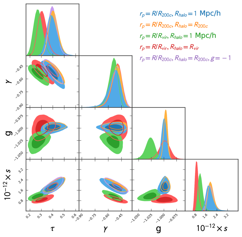
Figure 14: Posterior distribution of shape parameters in a benchmark bin of $M_{\rm 200c}/M_{\rm vir}\in[2\times 10^{14},5\times 10^{14})$ at $z=0.00$ under different binning schemes $r_{p}$ and $N_{\rm gal}$ models with different halo boundaries $R_{\rm halo}$. The marginalized parameter constraints for the full model closely overlap one another, and using the reduced model with $g=-1$ marginally improves the posterior constraints. The plot was generated using pygtc (Bocquet & Carter, 2016).

For the full model, we choose the error function as our fiducial functional form. The estimated parameters for both the full and reduced models are presented in Table 6 and Table 7, respectively. Appendix C provides robustness testing to determine the best-fit model for our covariance. In Table 6, we compare the model parameters, $\chi^{2}$ p-value, and the difference in Deviance Information Criterion (DIC) with our fiducial model using the candidate functions listed in Table 5. The error function generally outperforms other models when all parameters $\boldsymbol{\theta}\in\{\tau,\gamma,g,s\}$ are allowed to vary. Table 7 shows that the DIC of the reduced error function ($g=-1$) marginally outperforms the full error function in most cases, along with the posterior constraints of parameters shown in Figure 14.

Parameters	Priors
	Full	Reduced
$\tau$	Uniform (0, 10)	Uniform (0, 10)
$\gamma$	Uniform (-5, 5)	Uniform (-5, 5)
$g$	Uniform (-2, 1)	Fixed at $g=-1$
$10^{-12}\times s$	Log-uniform (0.01, 10)	Log-uniform (0.01, 10)

Table 4: Priors for the model. We introduce two sets of priors. In the "full" models, the parameters are given physical (i.e., $\tau>0$, $s>0$) but non-informative uniform or log-uniform priors. In the “reduced” case, assuming that Cov$(\Delta\Sigma,\ln N_{\rm gal}\mid M,z)=0$ at large scales, we restrict $g=-1$ while assigning the same set of priors to all other parameters.

Error function (fiducial)	$s\Big{(}{\rm erf}$$(\frac{\sqrt{\pi}}{2}\tilde{x})+g\Big{)}$
Logistics function	$s\Big{(}\frac{2}{1+e^{\tilde{x}}}-1+g\Big{)}$
Inverse tangent	$s\Big{(}\frac{2}{\pi}\arctan\big{(}\frac{\pi}{2}\tilde{x}\big{)}+g\Big{)}$
Algebraic second order	$s(\tilde{x}/(1+\tilde{x}^{2})^{1/2}+g)$

Table 5: Functional forms to model Cov($\Delta\Sigma$, $\ln N_{\rm gal}$). The radius in log-space $x$ is transformed to $\tilde{x}\equiv(x-\gamma)/\tau$ by a horizontal offset $\gamma$ and a characteristic scale $\tau$. The functions $f(\tilde{x})$ are normalized so that $f(\tilde{x})$ asymptotically goes to 1 at $+\infty$, -1 at $-\infty$, $f(0)=0$ and $f^{\prime}(0)=1$. Finally, we wrap $f(\tilde{x})$ by the function $p(f(\tilde{x}))\equiv s(f(\tilde{x}+g)$ to include a vertical offset $g$ and vertical scale $s$. Together $\mathbf{\theta}\in\{\tau,\gamma,g,s\}$ form the set of model parameters that allow us to make apple-to-apple comparisons between models.

Appendix B Particle Resolution and its impact on measurement errors

Using the 300 Cori Haswell node hours allocated by the NERSC to this project, we measured $\Delta\Sigma$ for $\sim 5000$ clusters using dark matter particles downsampled by a factor of 10, in 20 log-spaced radial bins, at a projection depth of $200~{}h^{-1}\rm Mpc$.

At a downsampling rate of 10, our effective dark matter particle resolution is $M_{\rm p}\approx 1.51\times 10^{10}h^{-1}M_{\odot}$. The error in $\Delta\Sigma$ comes from three sources: (i) cosmic variance, (ii) Poisson noise, and (iii) the intrinsic diversity of halos accounted for by secondary halo properties. In §6.2, we presented the contribution to $\Delta\Sigma$ scatter from secondary halo properties. Here, we compare the Poisson noise to the cosmic variance floor.

The cosmic variance introduces fluctuations in a 2D surface density fluctuation, given by

$$\delta\Delta\Sigma(R)=D_{p}\rho_{m}\sigma(R),$$ (35)

where $D_{p}=200h^{-1}\rm Mpc$ is the projection depth, $\rho_{m}(z)$ is the mean density of the universe at that redshift, and $\sigma(R)$ is the root mean squared matter density fluctuation, given by

$$\sigma^{2}(R)=\int\Delta^{2}(k)\Big{(}\frac{3j_{1}(kR)}{kR}\Big{)}^{2}d\ln{k},$$ (36)

which is smoothed over an area of $A=4\pi R^{2}$, $\Delta^{2}(k)$ is the matter power spectrum for a wavenumber $k$, and $j_{1}$ is the Bessel function of the first order.

Figure 13 shows the standard error of $\Delta\Sigma$ at a benchmark bin $M_{\rm 200c}\in[1\times 10^{14},2\times 10^{14})M_{\odot}h^{-1}$ at z=0.00. At particle downsampling factors of 200, 100, and 10, the reduction in error is consistent with the Poisson term of $\sqrt{N}$, indicating that at these sampling rates, Poisson noise dominates. At our current downsampling rate of nth=10, the standard error is just above the cosmic variance floor at small scales and drops below the cosmic variance floor at large scales. In the ideal case that Poisson noise accounts for all the standard error, fully sampling all particles (nth=1, red dotted line) will reduce the standard error by a factor of $\sqrt{10}$, rendering it just below the cosmic variance floor at small scales. In the realistic case that the standard error for $\Delta\Sigma$ contributes from both Poisson noise and the intrinsic diversity of halo profiles, the fully sampled standard error should be on par with the cosmic variance at small scales. A future study with fully sampled particles should yield greater statistical constraints.

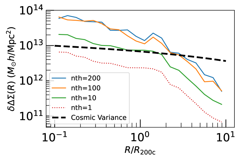
Figure 13: The standard error of $\Delta\Sigma$ measurements tested on a benchmark bin of $M_{\rm 200c}\in[1\times 10^{14},2\times 10^{14})M_{\odot}h^{-1}$ at z=0. The standard error is estimated using the bootstrap method for the $N=500$ clusters with dark matter particles downsampled by a factor of 200, 100, and 10 (solid lines). At our current resolution (nth=10, solid green line), the standard error is just above the cosmic variance at small scales and drops below the cosmic variance at large scales. The solid black line is density fluctuation estimated from the cosmic variance floor, as described in Equations (36) and (35). In the ideal case that Poisson noise accounts for all the standard error, fully sampling all particles ($n{\rm th}=1$, red dotted line) will reduce the standard error by a factor of $\sqrt{10}$, rendering it just below the cosmic variance floor at small scales. In the realistic case that the standard error for $\Delta\Sigma$ contributes from both Poisson noise and the intrinsic diversity of halo profiles, the fully sampled standard error should be on par with the cosmic variance at small scales.

Appendix C Robustness testing of Covariance Modeling

The shape posterior is sampled by a Monto Carlo Markov Chain (MCMC) using the emcee package (Foreman-Mackey et al., 2013). We test for convergence by ensuring that the number of steps exceeds $t_{\rm auto}/100$ for all parameters, where $t_{\rm auto}$ is the integrated autocorrelation time as defined by Goodman & Weare (2010) and by ensuring that the convergence diagnostic denoted with $R$ (Gelman & Rubin, 1992) across all walkers satisfy $R<1.05$.

The posterior distribution according to Bayes theorem is given as:

$$p(\boldsymbol{\theta}|\{y_{i}\}) \propto p({\{y_{i}\}|\boldsymbol{\theta}})p({\boldsymbol{\theta}})$$ (37)

$$=\prod_{i}p({y_{i}|\boldsymbol{\theta}})p({\boldsymbol{\theta}}),$$ (38)

where the second line assumes independent and identical distribution ($\mathrm{i.i.d}$) for the data vectors. We set uniform priors $p({\boldsymbol{\theta}})$ shown in Table  4 with signs and ranges motivated by the shape of the covariance (i.e., a negative $\gamma$ and positive $\tau$ to offset $f(\tilde{x})$ to the left and a positive $s$ and negative $g$ shifts the fitted curve downwards).

We measure the goodness of fit using the left-tail $p$-value for the $\chi^{2}$ with $N_{\rm data}-N_{\rm dim}=20-4=16$ degrees of freedom. We compare between models by the Deviance Information Criterion defined as

$$\mathrm{DIC}=2\overline{D(\boldsymbol{\theta})}-D(\boldsymbol{\overline{\theta}}),$$ (39)

where $\overline{\theta}$ is the best-fit parameters, and $D(\boldsymbol{\theta})$ is defined as

$$D(\boldsymbol{\theta})\equiv-2\log{(P({\{x_{i}\}|\boldsymbol{\theta}}))}.$$ (40)

The performance between different functional forms (Table 5) is reported in Table 4.

The summary statistics for the posterior distribution of the covariance models are listed in Table 6 as plotted against measurements in Figure 4. Among the functions, the error function has either a better or comparable fit to all other functions in all other bins, as indicated by their DIC parameters. In two bins $M_{\rm 200c}\in[5\times 10^{14},1\times 10^{15})$ at $z=0.49$ and $M_{\rm 200c}\in[2\times 10^{14},5\times 10^{15})$ at $z=1.03$, the amplitude of the covariance is too small relative to their errors for shape parameters to be well-constrained. The right tail $p$-value for $\chi^{2}$ is $p>0.05$ for all but one bin. For this reason, we take the full error function as the nominal functional form.

For $R\geq R_{\rm vir}$ or $R\geq R_{\rm 200c}$, we find the covariance to be null at $p$-values $>0.01$. A zero covariance at large scales implies $g=-1$ which coincides with the reduced model. We compare the results of the error function of the reduced model to the full model and find their performance varies from bin to bin as indicated by the DIC (Table  7). The posteriors of the reduced model provide marginally tighter constraints than the full model (Figure 14).

Mass & redshift	Error function (full): $s\Big{(}{\rm erf}(\frac{\sqrt{\pi}}{2}\tilde{x})+g\Big{)}$
	$\tau$	$\gamma$	$g$	$10^{12}\times s$	$\Delta\rm DIC_{\rm log}$	$\Delta\rm DIC_{\rm alg}$	$\Delta\rm DIC_{\rm arctan}$	$p$-value
$[5\times 10^{13},1\times 10^{14})$, $z=0.00$	$0.47^{+0.06}_{-0.05}$	$-0.66^{+0.08}_{-0.11}$	$-0.99^{+0.005}_{+0.004}$	$2.88^{+0.71}_{-0.47}$	4.8	17.8	31.5	0.27
$[1\times 10^{14},2\times 10^{14})$, $z=0.00$	$0.57^{+0.11}_{-0.08}$	$-0.76^{+0.14}_{-0.22}$	$-1.008^{+0.0005}_{-0.0007}$	$2.73^{+0.13}_{-0.65}$	-2.9	-1.7	2.8	0.88
$[2\times 10^{14},5\times 10^{14})$, $z=0.00$	$0.41^{+0.04}_{-0.04}$	$-0.51^{+0.05}_{-0.06}$	$-0.997^{+0.004}_{-0.0004}$	$1.93^{+0.24}_{-0.18}$	4.4	17.4	35.0	0.79
$[5\times 10^{14},1\times 10^{15})$, $z=0.00$	$0.27^{+0.03}_{-0.03}$	$-0.40^{+0.04}_{-0.05}$	$-1.006^{+0.005}_{-0.0005}$	$1.03^{+0.13}_{-0.11}$	-0.27	14.3	29.1	0.0009
$[5\times 10^{13},1\times 10^{14})$, $z=0.49$	$0.28^{+0.6}_{-0.05}$	$-0.36^{+0.05}_{-0.07}$	$-0.990^{+0.013}_{-0.013}$	$0.75^{+0.11}_{-0.09}$	2.7	9.0	15.1	0.72
$[1\times 10^{14},2\times 10^{14})$, $z=0.49$	$0.35^{+0.07}_{-0.06}$	$-0.43^{+0.07}_{-0.09}$	$-1.022^{+0.016}_{-0.017}$	$0.81^{+0.15}_{-0.10}$	1.7	5.4	9.3	0.97
$[2\times 10^{14},5\times 10^{14})$, $z=0.49$	$0.24^{+0.08}_{-0.07}$	$-0.49^{+0.07}_{-0.10}$	$-0.995^{+0.012}_{-0.011}$	$0.51^{+0.14}_{-0.01}$	0.6	2.4	4.0	0.63
$[5\times 10^{14},1\times 10^{15})$, $z=0.49$	NA
$[5\times 10^{13},1\times 10^{14})$, $z=1.03$	$0.17^{+0.05}_{-0.04}$	$-0.31^{+0.05}_{-0.05}$	$-1.019^{+0.020}_{-0.022}$	$0.35^{+0.06}_{-0.05}$	4.3	6.5	8.3	0.05
$[1\times 10^{14},2\times 10^{14})$, $z=1.03$	$0.21^{+0.06}_{-0.05}$	$-0.42^{+0.05}_{-0.06}$	$-1.024^{+0.013}_{-0.0014}$	$0.51^{+0.09}_{-0.07}$	-0.3	3.3	6.1	0.01
$[2\times 10^{14},5\times 10^{14})$, $z=1.03$	NA

Table 6: Summary statistics for Cov($\Delta\Sigma$, $N_{\rm gal}\mid M,z$) binned by $R_{\rm 200c}$ and $M_{200c}$, with $N_{\rm gal}$ defined inside the halo $R_{\rm 200c}$. Columns 2-5 are the best-fit parameters for the nominal error function and their $1\sigma$ ranges. Columns 6-8 are the difference between the DIC of the logistics, algebraic, and inverse tangent models with the nominal error function, respectively. Column 9 is the right-tail p-value as measured by the $\chi^{2}$ statistic with 20-4 = 16 degrees of freedom. Across all bins with applicable posterior constraints, the error function out-performs or is comparable to alternative functional forms as indicated by the difference in DIC, and has $p\geq 0.01$ in all but one bin. In two bins $M_{\rm 200c}\in[5\times 10^{14},1\times 10^{15})$ at $z=0.49$ and $M_{\rm 200c}\in[2\times 10^{14},5\times 10^{15})$ at $z=1.03$ the size of the covariance is too small relative to the size of their errors for shape parameters to be constrained. The covariance in these two bins is consistent with null at $p=0.01$ and $p=0.05$ levels, respectively.

Mass & redshift	Error function (reduced): $s\Big{(}{\rm erf}(\frac{\sqrt{\pi}}{2}\tilde{x})-1\Big{)}$
	$\tau$	$\gamma$	$10^{12}\times s$	$\Delta\rm DIC_{\rm erf-full}$	$p$-value
$[5\times 10^{13},1\times 10^{14})$, $z=0.00$	$0.44^{+0.04}_{-0.04}$	$-0.63^{+0.07}_{-0.09}$	$2.66^{+0.56}_{-0.39}$	-5.2	0.06
$[1\times 10^{14},2\times 10^{14})$, $z=0.00$	$0.69^{+0.11}_{-0.09}$	$-0.98^{+0.20}_{-0.27}$	$4.10^{2.31}_{1.19}$	4.5	0.96
$[2\times 10^{14},5\times 10^{14})$, $z=0.00$	$0.40^{+0.04}_{-0.03}$	$-0.50^{+0.05}_{-0.06}$	$1.90^{+0.26}_{-0.20}$	0.2	0.78
$[5\times 10^{14},1\times 10^{15})$, $z=0.00$	$0.29^{+0.04}_{-0.04}$	$-0.40^{+0.04}_{-0.04}$	$1.12^{+0.13}_{-0.11}$	6.1	0.005
$[5\times 10^{13},1\times 10^{14})$, $z=0.49$	$0.25^{+0.04}_{-0.03}$	$-0.35^{+0.04}_{-0.04}$	$0.79^{+0.08}_{-0.07}$	6.2	0.57
$[1\times 10^{14},2\times 10^{14})$, $z=0.49$	$0.38^{+0.14}_{-0.09}$	$-0.48^{+0.12}_{-0.24}$	$0.85^{+0.46}_{-0.19}$	-6.9	0.81
$[2\times 10^{14},5\times 10^{14})$, $z=0.49$	$0.25^{+0.21}_{-0.12}$	$-0.55^{+0.14}_{-0.42}$	$0.40^{+0.69}_{-0.13}$	NA	0.48
$[5\times 10^{14},1\times 10^{15})$, $z=0.49$	$0.61^{+0.27}_{-0.24}$	$-0.90^{+0.49}_{-0.76}$	$1.01^{+3.05}_{-0.60}$	-5.7	0.99
$[5\times 10^{13},1\times 10^{14})$, $z=1.03$	$0.20^{+0.06}_{-0.05}$	$-0.35^{+0.06}_{-0.08}$	$0.38^{+0.07}_{-0.06}$	-0.75	0.04
$[1\times 10^{14},2\times 10^{14})$, $z=1.03$	$0.22^{+0.06}_{-0.05}$	$-0.42^{+0.06}_{-0.8}$	$0.54^{+0.11}_{-0.09}$	3.9	0.3
$[2\times 10^{14},5\times 10^{14})$, $z=1.03$	$5.97^{+2.76}_{-3.01}$	$-0.55^{+3.30}_{-2.99}$	$0.02^{+0.02}_{-0.008}$	NA	0.15

Table 7: Summary statistics for Cov($\Delta\Sigma,N_{\rm gal}\mid M,z$) binned by $R_{\rm 200c}$ and $M_{200c}$ with $N_{\rm gal}$ defined inside the halo $R_{\rm 200c}$ for the reduced error function model. Compared with the full error function model, the performance of the reduced model varies from bin to bin – using $\Delta{\rm DIC}>3$ as a statistically significant result, it outperforms the full model in 5/9 overlapping bins, under-performs in 3/9 bins, and is comparable in 2 bins. The reduced model is able to yield convergent chains for $M_{\rm 200c}\in[5\times 10^{14},1\times 10^{15})$ at $z=0.49$ and $M_{\rm 200c}\in[2\times 10^{14},5\times 10^{15})$ at $z=1.03$ but with poor constraints on the parameters.

Redshift	$R^{2}$	Const	$c_{\rm vir}$		T/|U|		$a_{1/2}$		$\Gamma^{*}_{\rm 2dyn}$		$X_{\rm off}$
& $M_{\rm 200c}$ ($M_{\odot}h^{-1}$)			$\beta_{N_{\rm gal}}$	$F$	$\beta_{N_{\rm gal},}$	$F$	$\beta_{N_{\rm gal}}$	$F$	$10^{6}\times\beta_{N_{\rm gal}}$	$F$	$10^{3}\times\beta_{N_{\rm gal}}$	$F$
$z=0.00$
$[5\times 10^{13},1\times 10^{14})$	0.45	-0.69	-0.035(0.004)	171	1.448(0.135)	185	0.103(0.084)	166	2.743(1.68)	134	-1.62(0.23)	69
$[1\times 10^{14},2\times 10^{14})$	0.48	-0.46	-0.033(0.003)	217	1.086(0.120)	179	-0.198(0.071)	170	2.668(0.628)	206	-0.76(0.15)	86
$[2\times 10^{14},5\times 10^{14})$	0.49	-0.41	-0.029(0.003)	196	-0.794(0.086)	145	0.292(0.007)	213	-0.722(0.223)	167	0.57(0.11)	67
$[5\times 10^{14},1\times 10^{15})$	0.46	-0.32	-0.019(0.002)	119	1.503(0.068)	111	0.148(0.054)	201	0.483(0.096)	226	-0.25(0.06)	51
$z=0.49$
$[5\times 10^{13},1\times 10^{14})$	0.25	-0.71	0.006(0.005)	24	0.325(0.125)	69	0.188(0.101)	142	3.90(1.64)	102	-0.3(0.19)	35
$[1\times 10^{14},2\times 10^{14})$	0.21	-0.45	-0.450(0.082)	27	0.314(0.135)	46	-0.353(0.158)	107	1.80(0.71)	89	-0.37(0.13)	14
$[2\times 10^{14},5\times 10^{14})$	0.13	-0.56	-0.003(0.004)	0	0.323(0.110)	26	0.670(0.155)	51	0.388(0.108)	26	-0.27(0.11)	2
$[5\times 10^{14},1\times 10^{15})$	0.13	-0.32	-0.010(.008)	0	0.007(0.286)	0	0.697(.309)	5	-0.538(0.331)	3	-0.41(.14)	3
$z=1.03$
$[5\times 10^{13},1\times 10^{14})$	0.27	-1.12	0.015(0.005)	6	0.471(0.136)	21	0.569(0.269)	116	2.7(1.2)	63	-0.81(0.18)	0
$[1\times 10^{14},2\times 10^{14})$	0.22	-0.84	0.016(0.004)	10	0.374(0.135)	36	-0.233(0.234)	83	1.076(0.478)	36	-0.35(0.12)	2
$[2\times 10^{14},5\times 10^{14})$	0.20	-0.6	0.0015(0.005)	10	0.284(0.185)	1	-0.157(0.266)	15	0.160(0.213)	6	-0.55(0.11)	13

Table 8: Best-fit parameters, global $R^{2}$, and explanatory power indicators for log-richness modeled in Equation (22). Values in parentheses represent $1\sigma$ confidence intervals to the partial slopes $\beta$. The partial $F$-statistic, defined in Equation (41), is used to quantify the explanatory power of each variable. A higher partial F-statistic indicates a greater amount of predictive power uniquely attributed to that variable. Statistical significance is determined by an F-statistic of $F>10$.

Appendix D Modeling Secondary Properties

We describe the linear regression model for richness used in §6.1. The same methodology is applied to $\Delta\Sigma$ in §6.2.

To model the expected natural logarithm of galaxy count ($\ln N_{\rm gal}$), we decompose it linearly using secondary halo parameters listed in Table 3, as shown in Equation (22). We employ the least squares method for linear regression and examine parameter redundancies. For over half of the bins, the parameters $\Gamma_{\rm inst}$, $\Gamma_{\rm 100Myr}$, $\Gamma_{\rm 2dyn}$, and $\Gamma_{\rm peak}$ exhibit collinearity, with Variance Inflation Factors (VIF) exceeding 5. This outcome is expected, as these quantities represent the same physical quantities smoothed over different time scales. As for the reduced set of non-collinear parameters, their correlation coefficient are quantified in Shin & Diemer (2023) using the Erebos simulation suite. To determine which parameters to retain, we utilize the partial F-statistic.

Table 8 demonstrates the diminishing explanatory power of $\Pi$ on the richness as seen by the diminishing $R^{2}$ and $F_{\rm partial}$. We consider the partial F-statistic serves as a heuristic measure for the explanatory power of a variable, defined as:

$$F_{\rm partial}=\frac{({\rm RSSE_{\rm reduced}-RSSE_{\rm full}})/p}{{\rm RSSE_{\rm full}}/(n-k)},$$ (41)

where RSSE is the residual sum of squared errors for the reduced model after removing the parameter in question and the full model containing $\Pi\subset~{}\{a_{1/2},c_{\rm vir},T/U,\Gamma_{\rm 2dyn},X_{\rm off}\}$, $p$ is the number of parameters removed from the full model which in our case is by construction set to $p=1$, $n$ the number of data points, and $k$ is the number of parameters in the full backward model. This statistic can be shown to be proportional to the contribution to the total $R^{2}$ uniquely explained by this parameter alone.

A partial F-statistic test reveals that $\Gamma_{\rm 2dyn}$ exhibits the highest partial F-statistic. Therefore, we retain this parameter in the reduced dimensional linear regression. The final model includes the following parameters $\Pi\subset\{a_{1/2},c_{\rm vir},T/U,\Gamma_{\rm 2dyn},X_{\rm off}\}$. To ensure the robustness of the linear model across all bins, we perform the following tests:

• Variance inflation factor (VIF) test with a cutoff of 5 to detect multicollinearity.

• Global F-statistic for the entire model with a significance level of $0.05$ to examine the correlation between the dependent variable and all parameters.

• Partial F-statistic for the entire parameter set to compare the relative importance of each parameter. The Partial F-statistic measures the additional contribution of each parameter to the multi-linear fit by estimating its corresponding $R^{2}$ value.

• T-statistic for each parameter to verify that the coefficients significantly deviate from zero at a significance level of $0.05$.

• Breusch-Pagan Lagrange Multiplier test (Breusch & Pagan, 1979) at a significance level of $0.05$ to assess heteroscedasticity.

• Shapiro-Wilk test (Shapiro & Wilk, 1965) at a significance level of $0.05$ to evaluate the Gaussianity of residuals.

Across all bins, the reduced model successfully satisfies the first four tests. However, some bins fail the Shapiro-Wilk test due to a negative skew and positive kurtosis. Nonetheless, a visual examination of Q-Q plots indicates that the residuals predominantly follow a Gaussian distribution, except for deviations at the tail ends. Q-Q plots, quantile-quantile plots, are visualization tools used to compare the quantiles of a dataset to the quantiles of a theoretical distribution, typically a normal distribution. They provide a visual assessment of how well the data aligns with the assumed distribution.

References

- Abbott et al. (2018) Abbott T., et al., 2018, Physical Review D, 98
- Aguena et al. (2021) Aguena M., et al., 2021, Monthly Notices of the Royal Astronomical Society, 508, 6092
- Allen et al. (2011) Allen S. W., Evrard A. E., Mantz A. B., 2011, ARA&A, 49, 409
- Allgood et al. (2006) Allgood B., Flores R. A., Primack J. R., Kravtsov A. V., Wechsler R. H., Faltenbacher A., Bullock J. S., 2006, MNRAS, 367, 1781
- Anbajagane et al. (2020) Anbajagane D., Evrard A. E., Farahi A., Barnes D. J., Dolag K., McCarthy I. G., Nelson D., Pillepich A., 2020, MNRAS, 495, 686
- Anbajagane et al. (2022) Anbajagane D., Evrard A. E., Farahi A., 2022, MNRAS, 509, 3441
- Applegate et al. (2014) Applegate D. E., et al., 2014, MNRAS, 439, 48
- Baldry et al. (2012) Baldry I. K., et al., 2012, Monthly Notices of the Royal Astronomical Society, pp no–no
- Behroozi et al. (2013) Behroozi P. S., Wechsler R. H., Wu H.-Y., 2013, ApJ, 762, 109
- Bhattacharya et al. (2011) Bhattacharya S., Heitmann K., White M., Lukić Z., Wagner C., Habib S., 2011, ApJ, 732, 122
- Blanchard & Ilić (2021) Blanchard A., Ilić S., 2021, A&A, 656, A75
- Bocquet & Carter (2016) Bocquet S., Carter F. W., 2016, The Journal of Open Source Software, 1
- Bocquet et al. (2016) Bocquet S., Saro A., Dolag K., Mohr J. J., 2016, MNRAS, 456, 2361
- Breusch & Pagan (1979) Breusch T., Pagan A., 1979, Econometrica, 47, 1287
- Bryan & Norman (1998) Bryan G. L., Norman M. L., 1998, ApJ, 495, 80
- Chiu et al. (2020) Chiu I. N., Umetsu K., Murata R., Medezinski E., Oguri M., 2020, MNRAS, 495, 428
- Costanzi et al. (2019) Costanzi M., et al., 2019, MNRAS, 482, 490
- Costanzi et al. (2021) Costanzi M., et al., 2021, Phys. Rev. D, 103, 043522
- Croton et al. (2016) Croton D. J., et al., 2016, ApJS, 222, 22
- Dark Energy Survey Collaboration et al. (2016) Dark Energy Survey Collaboration et al., 2016, MNRAS, 460, 1270
- Despali et al. (2016) Despali G., Giocoli C., Angulo R. E., Tormen G., Sheth R. K., Baso G., Moscardini L., 2016, MNRAS, 456, 2486
- Diemer & Joyce (2019) Diemer B., Joyce M., 2019, ApJ, 871, 168
- Diemer & Kravtsov (2014) Diemer B., Kravtsov A. V., 2014, ApJ, 789, 1
- Dodelson et al. (2016) Dodelson S., Heitmann K., Hirata C., Honscheid K., Roodman A., Seljak U., Slosar A., Trodden M., 2016, arXiv e-prints, p. arXiv:1604.07626
- Euclid Collaboration et al. (2019) Euclid Collaboration et al., 2019, A&A, 627, A23
- Evrard et al. (2014) Evrard A. E., Arnault P., Huterer D., Farahi A., 2014, MNRAS, 441, 3562
- Farahi et al. (2016) Farahi A., Evrard A. E., Rozo E., Rykoff E. S., Wechsler R. H., 2016, MNRAS, 460, 3900
- Farahi et al. (2018) Farahi A., Evrard A. E., McCarthy I., Barnes D. J., Kay S. T., 2018, MNRAS, 478, 2618
- Farahi et al. (2019) Farahi A., et al., 2019, Nature Communications, 10, 2504
- Farahi et al. (2020) Farahi A., Ho M., Trac H., 2020, MNRAS, 493, 1361
- Farahi et al. (2022a) Farahi A., Anbajagane D., Evrard A. E., 2022a, ApJ, 931, 166
- Farahi et al. (2022b) Farahi A., Nagai D., Anbajagane D., 2022b, ApJ, 933, 48
- Foreman-Mackey et al. (2013) Foreman-Mackey D., Hogg D. W., Lang D., Goodman J., 2013, PASP, 125, 306
- Gelman & Rubin (1992) Gelman A., Rubin D. B., 1992, Statistical Science, 7, 457
- Giodini et al. (2013) Giodini S., Lovisari L., Pointecouteau E., Ettori S., Reiprich T. H., Hoekstra H., 2013, Space Science Reviews, 177, 247
- Golden-Marx & Miller (2018) Golden-Marx J. B., Miller C. J., 2018, ApJ, 860, 2
- Goodman & Weare (2010) Goodman J., Weare J., 2010, Communications in Applied Mathematics and Computational Science, 5, 65
- Hearin et al. (2013) Hearin A. P., Zentner A. R., Newman J. A., Berlind A. A., 2013, MNRAS, 430, 1238
- Huang et al. (2022) Huang S., et al., 2022, MNRAS, 515, 4722
- Ivezić et al. (2019) Ivezić Ž., et al., 2019, ApJ, 873, 111
- Johnston et al. (2007) Johnston D. E., et al., 2007, arXiv e-prints, p. arXiv:0709.1159
- Kettula et al. (2015) Kettula K., et al., 2015, MNRAS, 451, 1460
- Kiiveri et al. (2021) Kiiveri K., et al., 2021, MNRAS, 502, 1494
- Klypin et al. (2016) Klypin A., Yepes G., Gottlöber S., Prada F., Heß S., 2016, MNRAS, 457, 4340
- Lau et al. (2015) Lau E. T., Nagai D., Avestruz C., Nelson K., Vikhlinin A., 2015, ApJ, 806, 68
- Lee et al. (2023) Lee W., et al., 2023, ApJ, 945, 71
- Lesci et al. (2022) Lesci G. F., et al., 2022, A&A, 665, A100
- Lokken et al. (2022) Lokken M., et al., 2022, ApJ, 933, 134
- Lu et al. (2006) Lu Y., Mo H. J., Katz N., Weinberg M. D., 2006, MNRAS, 368, 1931
- Ludlow et al. (2012) Ludlow A. D., Navarro J. F., Li M., Angulo R. E., Boylan-Kolchin M., Bett P. E., 2012, MNRAS, 427, 1322
- Mantz et al. (2010) Mantz A., Allen S. W., Ebeling H., Rapetti D., Drlica-Wagner A., 2010, MNRAS, 406, 1773
- Mantz et al. (2015) Mantz A. B., et al., 2015, MNRAS, 446, 2205
- Mantz et al. (2016a) Mantz A. B., Allen S. W., Morris R. G., Schmidt R. W., 2016a, MNRAS, 456, 4020
- Mantz et al. (2016b) Mantz A. B., et al., 2016b, MNRAS, 463, 3582
- Maraston et al. (2013) Maraston C., et al., 2013, MNRAS, 435, 2764
- McClintock et al. (2019) McClintock T., et al., 2019, MNRAS, 482, 1352
- Miyatake et al. (2022) Miyatake H., et al., 2022, Phys. Rev. D, 106, 083519
- Mulroy et al. (2019) Mulroy S. L., et al., 2019, MNRAS, 484, 60
- Murata et al. (2019) Murata R., et al., 2019, PASJ, 71, 107
- Nishimichi et al. (2019) Nishimichi T., et al., 2019, ApJ, 884, 29
- Nord et al. (2008) Nord B., Stanek R., Rasia E., Evrard A. E., 2008, MNRAS, 383, L10
- Percival (2005) Percival W. J., 2005, A&A, 443, 819
- Pierre et al. (2016) Pierre M., et al., 2016, A&A, 592, A1
- Pillepich et al. (2010) Pillepich A., Porciani C., Hahn O., 2010, MNRAS, 402, 191
- Planck Collaboration et al. (2014) Planck Collaboration et al., 2014, A&A, 571, A16
- Planck Collaboration et al. (2020) Planck Collaboration et al., 2020, A&A, 641, A6
- Prada et al. (2012) Prada F., Klypin A. A., Cuesta A. J., Betancort-Rijo J. E., Primack J., 2012, MNRAS, 423, 3018
- Pratt et al. (2019) Pratt G. W., Arnaud M., Biviano A., Eckert D., Ettori S., Nagai D., Okabe N., Reiprich T. H., 2019, Space Sci. Rev., 215, 25
- Press & Schechter (1974) Press W. H., Schechter P., 1974, ApJ, 187, 425
- Qu et al. (2023) Qu F. J., et al., 2023, The Atacama Cosmology Telescope: A Measurement of the DR6 CMB Lensing Power Spectrum and its Implications for Structure Growth (arXiv:2304.05202)
- Riebe et al. (2013) Riebe K., et al., 2013, Astronomische Nachrichten, 334, 691
- Rozo et al. (2010) Rozo E., et al., 2010, ApJ, 708, 645
- Rozo et al. (2014) Rozo E., Evrard A. E., Rykoff E. S., Bartlett J. G., 2014, MNRAS, 438, 62
- Rozo et al. (2015) Rozo E., Rykoff E. S., Becker M., Reddick R. M., Wechsler R. H., 2015, MNRAS, 453, 38
- Rykoff et al. (2014a) Rykoff E. S., et al., 2014a, ApJ, 785, 104
- Rykoff et al. (2014b) Rykoff E. S., et al., 2014b, ApJ, 785, 104
- Salcedo et al. (2020) Salcedo A. N., Wibking B. D., Weinberg D. H., Wu H.-Y., Ferrer D., Eisenstein D., Pinto P., 2020, MNRAS, 491, 3061
- Schrabback et al. (2018) Schrabback T., et al., 2018, MNRAS, 474, 2635
- Sereno et al. (2020) Sereno M., et al., 2020, MNRAS, 492, 4528
- Shapiro & Wilk (1965) Shapiro S. S., Wilk M. B., 1965, Biometrika, 52, 591
- Shin & Diemer (2023) Shin T., Diemer B., 2023, MNRAS, 521, 5570
- Somerville et al. (2001) Somerville R. S., Primack J. R., Faber S. M., 2001, MNRAS, 320, 504
- Stanek et al. (2010) Stanek R., Rasia E., Evrard A. E., Pearce F., Gazzola L., 2010, ApJ, 715, 1508
- Stark et al. (2009) Stark D. V., McGaugh S. S., Swaters R. A., 2009, AJ, 138, 392
- Sunayama (2023) Sunayama T., 2023, MNRAS, 521, 5064
- Sunayama et al. (2020) Sunayama T., et al., 2020, MNRAS, 496, 4468
- Tinker et al. (2008) Tinker J., Kravtsov A. V., Klypin A., Abazajian K., Warren M., Yepes G., Gottlöber S., Holz D. E., 2008, ApJ, 688, 709
- Tinker et al. (2010) Tinker J. L., Robertson B. E., Kravtsov A. V., Klypin A., Warren M. S., Yepes G., Gottlöber S., 2010, ApJ, 724, 878
- To et al. (2021) To C., et al., 2021, Phys. Rev. Lett., 126, 141301
- Tremonti et al. (2004) Tremonti C. A., et al., 2004, ApJ, 613, 898
- Vikhlinin et al. (2009) Vikhlinin A., et al., 2009, ApJ, 692, 1060
- Wang et al. (2022) Wang K., Mao Y.-Y., Zentner A. R., Guo H., Lange J. U., van den Bosch F. C., Mezini L., 2022, MNRAS, 516, 4003
- Watson et al. (2013) Watson W. A., Iliev I. T., D’Aloisio A., Knebe A., Shapiro P. R., Yepes G., 2013, MNRAS, 433, 1230
- Wechsler & Tinker (2018) Wechsler R. H., Tinker J. L., 2018, ARA&A, 56, 435
- Wechsler et al. (2002) Wechsler R. H., Bullock J. S., Primack J. R., Kravtsov A. V., Dekel A., 2002, ApJ, 568, 52
- Wu et al. (2015) Wu H.-Y., Evrard A. E., Hahn O., Martizzi D., Teyssier R., Wechsler R. H., 2015, MNRAS, 452, 1982
- Wu et al. (2022) Wu H.-Y., et al., 2022, MNRAS, 515, 4471
- Xhakaj et al. (2022) Xhakaj E., Leauthaud A., Lange J., Hearin A., Diemer B., Dalal N., 2022, MNRAS, 514, 2876
- Zentner et al. (2005) Zentner A. R., Berlind A. A., Bullock J. S., Kravtsov A. V., Wechsler R. H., 2005, ApJ, 624, 505
- Zentner et al. (2019) Zentner A. R., Hearin A., van den Bosch F. C., Lange J. U., Villarreal A. S., 2019, MNRAS, 485, 1196
- Zhang & Annis (2022) Zhang Y., Annis J., 2022, MNRAS, 511, L30
- Zhao et al. (2003) Zhao D. H., Jing Y. P., Mo H. J., Brner G., 2003, ApJ, 597, L9
- Zu et al. (2014) Zu Y., Weinberg D. H., Rozo E., Sheldon E. S., Tinker J. L., Becker M. R., 2014, MNRAS, 439, 1628
- de Haan et al. (2016) de Haan T., et al., 2016, ApJ, 832, 95
- von der Linden et al. (2014) von der Linden A., et al., 2014, MNRAS, 439, 2