The Milky Way in Context: Building an integral-field spectrograph data cube of the Galaxy

Abstract

The Milky Way (MW) is by far the best-studied galaxy and has been regarded as an ideal laboratory for understanding galaxy evolution. However, direct comparisons of Galactic and extra-galactic observations are marred by many challenges, including selection effects and differences in observations and methodology. In this study, we present a novel code GalCraft to address these challenges by generating mock integral-field spectrograph data cubes of the MW using simple stellar population models and a mock stellar catalog of the Galaxy derived from E-Galaxia. The data products are in the same format as external galaxies, allowing for direct comparisons. We investigate the ability of pPXF to recover kinematics and stellar population properties for an edge-on mock observation of the MW. We confirm that pPXF can distinguish kinematic and stellar population differences between thin and thick disks. However, pPXF struggles to recover star formation history, where the SFR is overestimated in the ranges between $2-4$ and $12-14$ Gyr compared to the expected values. This is likely due to the template age spacing, pPXF regularization algorithm, and spectral similarities in old population templates. Furthermore, we find systematic offsets in the recovered kinematics, potentially due to insufficient spectral resolution and the variation of line-of-sight velocity with $[\mathrm{M/H}]$ and age through a line-of-sight. With future higher resolution and multi-$[\mathrm{\alpha/Fe}]$ SSP templates, GalCraft will be useful to identify key signatures such as $[\mathrm{\alpha/Fe}]$-$[\mathrm{M/H}]$ distribution at different $R$ and $|z|$ and potentially measure radial migration and kinematic heating efficiency to study detailed chemodynamical evolution of MW-like galaxies.

1 Introduction

How galaxies formed and evolved remains one of the outstanding questions facing astrophysics today. Due to our unique vantage point, the Milky Way (MW) is by far the best-studied galaxy in the Universe. Precise astrometric data from Gaia (Gaia Collaboration et al., 2023) and accurate chemical abundances of individual stars from large spectroscopic surveys such as LAMOST (Zhao et al., 2012), GALAH (Buder et al., 2021) and APOGEE (Majewski et al., 2017) have been conducted in the last decade for Galactic archaeologists to reveal the detailed chemodynamical picture of the Milky Way (Freeman & Bland-Hawthorn, 2002; Bland-Hawthorn & Gerhard, 2016). This includes the accretion history and interplay of chemical and dynamical processes (e.g., Xiang & Rix 2022). Particularly, Hayden et al. (2015) demonstrated two distinct sequences in $[\mathrm{\alpha/Fe}]$-$[\mathrm{Fe/H}]$ distributions with the fractions vary systematically with location $R$ and $|z|$ across the MW (see also Nidever et al. 2014), and the skewness of the outer-disk metallicity distribution function (MDF) indicates the important process of radial migration. The two $[\mathrm{\alpha/Fe}]$ sequences (also called $[\mathrm{\alpha/Fe}]$-bimodality) are associated with the thick and thin disks of the MW and are key diagnostics for understanding the MW’s chemodynamical evolution history.

In the past decades, many efforts have been made to develop Galactic chemical evolution (GCE) models to reproduce the $[\mathrm{\alpha/Fe}]$ bimodality and uncover its origin. The two-infall model (originally from Chiappini et al. 1997 and modified later by Haywood et al. 2018; Spitoni et al. 2019; Lian et al. 2020) assumes two distinct infall episodes with a delay of $4\sim 6$ Gyr. The first episode happens at the beginning of the model and forms metal-poor and $[\mathrm{\alpha/Fe}]$-enhanced stars. When the metallicity is enriched to $\sim 0.4$ dex, the second infall brings in metal-poor gas and resets gas’s chemical composition. Then the chemical enrichment repeats and $[\mathrm{\alpha/Fe}]$-poor stars spread along a wide range of metallicities. On the contrary, another theory by Schönrich & Binney (2009); Sanders & Binney (2015) considers radial migration or radial mixing. They showed that the extended $[\mathrm{Fe/H}]$ distribution in low-$[\mathrm{\alpha/Fe}]$ regime is due to radial migration where stars change their angular momentum or guiding radius with time, and one smooth episode of gas infall is sufficient to produce $[\mathrm{\alpha/Fe}]$-bimodality. The effect of radial migration is also seen in simulations (e.g., Minchev et al. 2013; Kubryk et al. 2015). Sharma et al. (2021b) applied Shu distribution function (Shu, 1969) and extended the model in Sanders & Binney (2015) by adding the distribution of $[\mathrm{\alpha/Fe}]$ and a new prescription for velocity dispersion relation from Sharma et al. (2021a), and successfully reproduced the $[\mathrm{\alpha/Fe}]$-$[\mathrm{Fe/H}]$ bimodality distributions at different $R$ and $|z|$. They are quantitatively consistent with APOGEE observations in Hayden et al. (2015). The relation of chemistry and kinematics is also consistent at all Galactic locations. In this study, we mainly focus on the model from Sharma et al. (2021a) and refer to the above-mentioned publications for details.

Even though specific chemical evolution models can reproduce the chemodynamical distributions of our MW successfully, it is still under debate what is the origin of $[\mathrm{\alpha/Fe}]$-bimodality. Because the MW is only one galaxy, whether these theories apply to other disk galaxies’ formation history or whether the MW is unique in the Universe is still an open question. For example, Mackereth et al. (2018) found $[\mathrm{\alpha/Fe}]$ bimodality is rare in the EAGLE simulation, while Buck (2020) found it to be present due to gas-rich mergers in all simulated MW-like galaxies from the NIHAO-UHD project. Therefore, it is essential to combine both the MW with other galaxies observations to answer these questions.

According to photometric and single-fiber spectroscopic observations on external galaxies, the MW from an extra-galactic view is an Sb-Sbc galaxy positioned at the “green valley" on the color-mass diagram (Mutch et al., 2011; Licquia et al., 2015) and obeys the Tully-Fisher relation (Licquia & Newman, 2016). It has a low star formation rate (SFR) which is not unusual when compared to similar galaxies (Fraser-McKelvie et al., 2019). The MW appears to be a normal spiral galaxy based on its kinematics and intrinsic luminosity (Bland-Hawthorn & Gerhard, 2016), but unusually compact for its stellar mass (e.g. Licquia et al. 2016). Its satellite galaxies are fewer in number and more compactly distributed (e.g. Yniguez et al. 2014) compared to other galaxies with similar total stellar mass. The geometric thin and thick disk structures obtained by vertically fitting the surface brightness profiles are found to be common in most disk galaxies (e.g., Yoachim & Dalcanton 2006; Comerón et al. 2018; Martínez-Lombilla & Knapen 2019), but whether they are related to different $[\mathrm{\alpha/Fe}]$ sequences were not investigated due to the lack of spatially resolved chemistry information.

Over the last decade, integral-field spectroscopy (IFS) instruments have enabled us to obtain integrated light spectra of galaxies across different regions of the same object. Several IFS surveys have already been carried out such as SAMI (Croom et al., 2012), CALIFA (Sánchez et al., 2012), and MaNGA (Bundy et al., 2015) to measure kinematics and chemical compositions of thousands of galaxies. Several studies compared face-on galaxies in these surveys with the MW: Boardman et al. (2020) selected 62 Milky Way analogs (MWAs) from MaNGA with the criteria of stellar masses and bulge-to-total ratios. They found most of these galaxies have flatter stellar and gas-phase metallicity gradients due to different disc scale lengths. A greater consistency can be found when scaling gradients by these lengths; Zhou et al. (2023) revisited 138 MaNGA galaxies by fitting the spectra with a semi-analytic chemical evolution model (Zhou et al., 2022) and measured their star formation and chemical enrichment histories. They detected similar $[\mathrm{\alpha/Fe}]$ bimodality as the Galactic APOGEE observations (Abdurro’uf et al., 2022) in many of the galaxies.

Even though face-on MWAs are ideal for measuring age and metallicity variations crossing different Galactocentric radii $R_{\mathrm{gc}}$, they lack vertical $(|z|)$ information, which is essential to geometrically distinguish the thin and thick disks and study their differences in chemical abundances. Therefore, edge-on MWAs are more useful in this case to provide elemental abundance distributions at different $R$ and $|z|$. Several studies of nearby edge-on MWAs and lenticular galaxies using MUSE found similar kinematics and bimodal distributions to the MW (e.g., Pinna et al. 2019a, b; Scott et al. 2021; Martig et al. 2021). In particular, Scott et al. (2021) demonstrated that UGC 10738 has similar $[\mathrm{\alpha/Fe}]$-$[\mathrm{Fe/H}]$ distributions at different projected $R$ and $|z|$ with the MW observation in Hayden et al. (2015) and model predictions in Sharma et al. (2021b), which supports the commonness of MW’s chemical distributions.

Despite the efforts above, a direct comparison of MW with its analogs in kinematics and chemistry is still challenging because the observables and methods used for studying the MW are different from those for external galaxies, i.e., utilizing properties of individual stars as opposed to integrated quantities with projection effects. Therefore, the comparisons may be impacted by systematics or biases (Boardman et al., 2020). In addition, some key processes such as radial migration and kinematic heating have not been extensively explored like the MW on external galaxies, which are also essential to identify whether the MW’s formation and evolution is distinct from the general population. Therefore, to take the MW as an ideal laboratory and test galaxy evolution theories, one needs to remove these observational and methodological biases, transfer the observables of MW and external systems into the same definition, and apply models that consider both chemical enrichment and kinematic processes. These considerations lead to the development of the tools presented in this work.

In this study, we present a novel code GalCraft to generate mock integral-field spectrograph (IFS) data cubes of the MW with integrated spectra using simple stellar population (SSP) models and mock stellar catalog from E-Galaxia (Sharma et al. 2024, in perp), which is based on the chemodynamical model of Sharma et al. (2021b) (hereafter S21) that is most consistent to the current Galactic observations in both kinematics and chemistry. This mock data cube is in the same format as extragalactic IFS observations. It can be applied to extragalactic data analysis methods (e.g., the GIST pipeline Bittner et al. 2019 with pPXF Cappellari & Emsellem 2004; Cappellari 2017, 2023) to measure directly comparable parameters in (age, $[\mathrm{M/H}]$, $[\mathrm{\alpha/Fe}]$, $V_{\rm LOS}$, $\sigma$, $h_{3}$, $h_{4}$). In addition, GalCraft can also be used to more comprehensively re-investigate the reliability of the above software in measuring kinematic and stellar population properties than before, because the inputs for generating mock data cubes are known. Therefore, we also address this topic in this work.

We describe the ingredients used in GalCraft and detailed procedures of this code in Section 2. In Section 3, we test the ability of spectral fitting tools to recover kinematics, stellar population parameters, and mass fraction distributions by applying it to a mock edge-on data cube and compare to the true values from E-Galaxia catalog. In Section 4, we discuss the causes of deviations between measured and true (input) values and address potential reasons and future improvements on current data reduction pipelines for obtaining better results. We explore the effect of different fitting strategies and provide some references when using spectral fitting tools. We also give some caveats about using GalCraft code. In Section 5, we talk about future plans on the improvements of GalCraft along with spectral fitting codes and prospect some scientific topics that can be done by using GalCraft. A summary is presented in Section 6.

2 Data Cube Generation

The purpose of GalCraft is to take the mock stellar catalog of the Galaxy obtained from E-Galaxia (Sharma et al. 2024, in prep.), and transform it into a mock data cube in three dimensions (two in spatial and one in spectral) as observed by integral-field spectrographs (IFS) such as MUSE (Bacon et al., 2010), SAMI (Croom et al., 2012) or MaNGA (Bundy et al., 2015). The GalCraft code takes as input the following set of user-specified input parameters: galaxy distance ($d$), inclination ($i$), extinction, SSP templates, instrumental properties, as well as a few additional parameters (see the full list in Table 1). The produced mock data cube can be processed in the same way as real IFS observations data by many methods, particularly codes like Voronoi binning (Cappellari & Copin, 2003), Penalized Pixel-Fitting (pPXF, Cappellari & Emsellem 2004; Cappellari 2017, 2023), line-strength indices (e.g., Worthey 1994; Schiavon 2007; Thomas et al. 2011; Martín-Navarro et al. 2018), or a combination of them (e.g., the GIST pipeline, Bittner et al. 2019). The results can be compared directly with those from IFS observations of MWAs in terms of mass- or light-weighted parameter maps, line-of-sight velocity distribution (LOSVD), and mass fraction distributions. The ingredients, flexibility, procedures, and computational expenses of this code are described in detail in the following sub-sections.

2.1 The Ingredients

2.1.1 Galactic Chemical Evolution Model

We apply the analytical chemodynamical model of the Milky Way developed by S21 which can predict the joint distribution of position $(\mathbf{x})$, velocity $(\mathbf{v})$, age $(\tau)$, extinction $E(B-V)$, the photometric magnitude in several bands and chemical abundances ($[\mathrm{Fe/H}]$, $[\mathrm{\alpha/Fe}]$) of stars in the Milky Way. Compared with previous models (e.g., Chiappini et al. 1997; Haywood et al. 2019), this model included a new prescription for the evolution of $[\mathrm{\alpha/Fe}]$ with age and $[\mathrm{Fe/H}]$ and a new set of relations describing the velocity dispersion of stars (Sharma et al., 2021a). This model shows for the first time that it can reproduce the $[\mathrm{\alpha/Fe}]$-$[\mathrm{Fe/H}]$ distribution of APOGEE observed stars (Hayden et al., 2015) at different radius $R$ and height $|z|$ across the Galaxy. In this model, the origin of two $[\mathrm{\alpha/Fe}]$ sequences is due to two key processes: the sharp transition from high-$[\mathrm{\alpha/Fe}]$ to low-$[\mathrm{\alpha/Fe}]$ at around 10.5 Gyr ago that creates a valley between the two sequences, which is likely due to the delay between the first star formation and sequential occurrence of SN Ia; the radial migration or so-called churning is responsible for the large spread of the low-$[\mathrm{\alpha/Fe}]$ sequence along the $[\mathrm{Fe/H}]$ axis. This model also showed that without churning it is not sufficient to reproduce the double sequences (see their Fig. 6). Because this chemical evolution model is purely analytical, it is easy to be inserted into the forward-modeling tool E-Galaxia to generate mock stellar catalogs for further analysis. In addition, several free parameters such as radial migration and heating efficiency are adjustable, which will be useful to implement similar analysis on external galaxies.

2.1.2 E-Galaxia

To mock the Milky Way IFS data cube, we need a comprehensive stellar catalog from observations on the Galaxy with well-measured parameters such as position $(\mathbf{x})$, velocity $(\mathbf{v})$, age $(\tau)$ and chemical abundances. However, this is impractical as the Galaxy has hundreds of billions of stars being unexplored and the dust in the disk obscures distant light. An alternative way is to use particle catalogs from N-body/hydrodynamical simulations (e.g., EAGLE Schaye et al. 2015, FIRE-2 Hopkins et al. 2018), but most of the simulations only contain $\sim 10^{6}$ stellar particles, which is not enough to generate integrated spectra because each spatial bin (spaxel) would only contain less than a hundred particles. This in turn would increase the sampling noise of the integrated spectrum and make observables derived from spectra noise. Even though oversampling can solve this problem, it is still challenging to find a simulation that is observably identical to the MW in all aspects quantitatively, especially the $[\mathrm{\alpha/Fe}]$ bimodal trends.

Therefore, the approach we take here is to generate a mock stellar catalog to represent the MW. We use E-Galaxia (Sharma et al. 2024, in prep.). This tool is in accordance with the chemical evolution model of S21 and can create a catalog with the user-defined number of particles ($N_{p}$) with parameters including position $(\mathbf{x,y,z})$, velocity $(\mathbf{v_{x},v_{y},v_{z}})$, age $(\tau)$, metallicity ($[\mathrm{M/H}]$) and $[\mathrm{\alpha/Fe}]$, where the parameter distributions are chemodynamically consistent to the MW observations. Other codes like TRILEGAL (Girardi et al., 2005), BESANCON (Girardi et al., 2005), and Galaxia (Sharma et al., 2011) can also create mock catalogs. However, compared to E-Galaxia, the underlying models of these codes lack the information of $[\mathrm{Fe/H}]$ and $[\mathrm{\alpha/Fe}]$, and do not have the processes of radial migration and kinematic heating. Furthermore, the ability of E-Galaxia to control the observed properties by regulating the underlying physical process is important for future analysis of external galaxies, whose formation history and dynamical processes are expected to be different from the Milky Way. One caveat is that star particles in the current version of E-Galaxia are distributed only in the disk and there is no bulge, halo, or nuclear disk structure. This is because the chemical and kinematic distribution functions predicted by S21 are extrapolated from observations in the solar neighborhood. Nevertheless, E-Galaxia parameter distributions are still consistent with APOGEE observations in the range of $3<R_{\rm{gc}}<15$ kpc.

2.1.3 Spectral Libraries

To build a mock data cube, one important procedure is to turn particles in E-Galaxia into stellar spectra based on their properties, so a spectra library is needed. Because the integrated light in extra-galactic observations is assumed from stellar populations, in GalCraft, we treat each particle as a single-stellar population (SSP). The SSP spectrum describes the spectral energy distribution (SED) of a stellar population with a single age, metallicity, and chemical abundance patterns. An initial mass function (IMF) is assumed, and the stellar population is evolved using a given isochrone (Conroy, 2013). GalCraft currently supports MILES (Vazdekis et al., 2010; Vazdekis et al., 2015) and PEGASE-HR (Le Borgne et al., 2004), both of which will be used in this study.

The MILES SSP library ($\rm{FWHM}=2.51\Angstrom$, $3500\Angstrom<\lambda<7500\Angstrom$) is based on the model of Vazdekis (1999). It uses Padova 2000 (Girardi et al., 2000) or BaSTI (Pietrinferni et al., 2004, 2006) isochrones and IMF in Unimodal/Bimodal (Vazdekis et al., 1996), Kroupa Universal/Revised (Kroupa, 2001) and Chabrier (Chabrier, 2003) shapes. For Padova 2000 isochrones, the template grids cover 7 metallicity bins between (-2.32, 0.22) dex, 50 age bins between (0.063, 17.78) Gyr and one scaled-solar $[\mathrm{\alpha/Fe}]$ bin (Vazdekis et al., 2010). As for BaSTI isochrones, the template grids cover 12 metallicity bins between (-2.27, 0.40) dex, 53 age bins between (0.03, 14.00) Gyr and two $[\mathrm{\alpha/Fe}]$ bins in 0.0 and 0.4 dex (Vazdekis et al., 2015). Since $[\mathrm{\alpha/Fe}]$ enhancement is essential in this study, for most of the cases we will use the $\alpha$-variable templates.

The PEGASE-HR library ($\rm{FWHM}=0.55\Angstrom$, $3900\Angstrom<\lambda<6800\Angstrom$) is based on the Elodie 3.1 stellar library (Prugniel & Soubiran, 2001; Prugniel et al., 2007). The SSP models are computed using Padova 1994 (Bertelli et al., 1994) isochrones with a Salpeter (Salpeter, 1955), Kroupa, or top-heavy (Elmegreen & Shadmehri, 2003) IMF. The templates grid consists of 7 metallicity bins between (-2.30, 0.70) dex, 68 age bins between (0.001, 20) Gyr, and one scaled-solar $[\mathrm{\alpha/Fe}]$ bin. In this work, the PEGASE-HR templates are mainly used to explore the effect of spectral resolution on pPXF fitting. Therefore, it is still useful even if it lacks variable $[\mathrm{\alpha/Fe}]$. Revised grids interpolated by ULYSS (Koleva et al., 2009) in the same way as Kacharov et al. (2018) for PEGASE-HR are also available. The new grids contain 15 steps in metallicity between -2.3 and 0.7 dex and 50 steps in age between 10 Myr and 14 Gyr.

2.2 Configurations of GalCraft

Table 1: Configuration parameters adjustable in the GalCraft code.

Parameters	Description	Unit
GALPARAMS:	Observation parameters of the Galaxy
distance	Distance of the Galaxy center to the observer	kpc
$\theta_{zx}$	Angles that the Galaxy rotates along the Y axis in the direction from $z$ to $x$	deg
$\theta_{yz}$	Angles that the Galaxy rotates along the X axis in the direction from $y$ to $z$	deg
$l$	Galactic longitude of the center of the Galaxy	deg
$b$	Galactic latitude of the center of the Galaxy	deg
SSPPARAMS:	Parameters of the SSP templates
model	The SSP model to be used for the spectrum (MILES or PEGASE-HR)
isochrone	Isochrones used to generate the SSP templates
IMF	Initial-mass function used to generate the SSP templates
single-alpha	If use single $[\mathrm{\alpha/Fe}]$ or $\alpha$-variable templates for the spectrum	bool
factor	Oversampling factor of the templates
$\rm FWHM_{-}gal$	Spectral resolution in FWHM of the output data cube	$\Angstrom$
dlam	Bin width of the wavelength sampling of the output data cube	$\Angstrom$
age-range	Optional age range (inclusive) in for the SSP models	Gyr
metal-range	Optional metallicity range (inclusive) in for the SSP models	dex
wave-range	Optional wavelength range (inclusive) in for the SSP models	$\Angstrom$
spec-interpolator	Interpolation method to assign the spectrum to the particle given its (age, metallicity, $[\mathrm{\alpha/Fe}]$)
INSPARAMS:	Instrument properties
instrument	Instrument name, when using this parameter, the other parameters will be automatically set
spatial-resolution	Spatial resolution of the data cube	arcsec
spatial-nbin	Number of spatial bins (spaxels) in two coordinates, in the format of [$n_{x}$, $n_{y}$]
FWHM-spatial	Full-Width Half-Maximum of the PSF function to model the atmosphere	arcsec

To meet different research purposes, we incorporated a wide range of adjustable parameters in GalCraft. Specifically, the adjustable parameters are divided into three groups: GALPARAMS, SSPPARAMS and INSPARAMS, as listed with descriptions in Table 1. The user can set up their preferred parameters to obtain the expected data cubes. GALPARAMS is for setting the distance, inclination, and position of the mock MW using coordinates transformation; SSPPARAMS governs the spectral properties, such as the SSP model selection, single or variable $[\mathrm{\alpha/Fe}]$, spectral resolution, age, $[\mathrm{M/H}]$ and wavelength range and the interpolation method to be used to assign each particle a spectrum (details in Section 2.3). Based on particles’ parameters, there are two options to assign them spectra: one is “nearest", which will assign the spectrum of the nearest template grid. The other is “linear", which will assign the spectrum by piece-wise linear interpolation of templates. The INSPARAMS controls the instrument spatial sampling, atmospheric effects (PSF), and the number of spatial bins in each coordinate. We also provide an option to derive the data cube in the format of a specified instrument. Alternatively, the user can also design a hypothetical instrument that does not exist by manually setting up these parameters, which will be useful for future instrument designs.

2.3 Procedures of Making a Mock Data-Cube

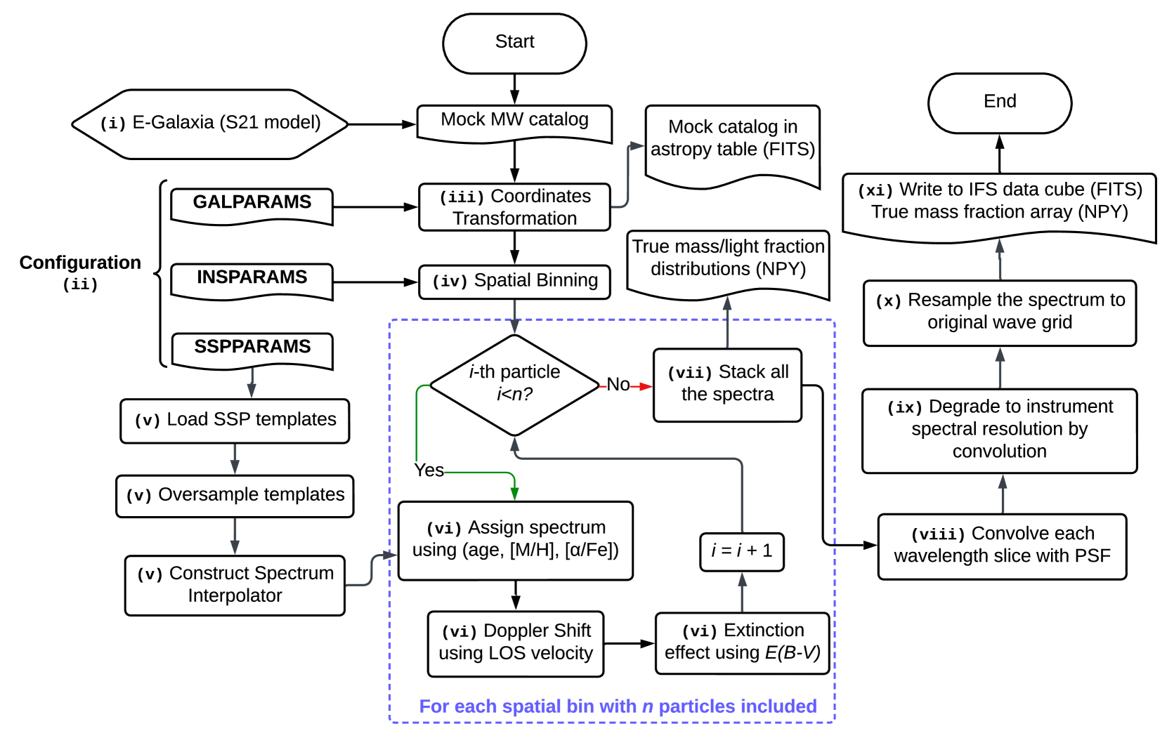
Figure 1: A flowchart that demonstrates the workflow of GalCraft code in this work. The numbers on some processes correspond to the steps listed in Section 2.3.

The procedures of generating mock MW data cubes are described in detail as the following steps, along with a flowchart in Fig. 1:

1. Use E-Galaxia to generate a mock stellar catalog of the MW, with particles’ position $(\mathbf{x})$, velocity $(\mathbf{v})$, age $(\tau)$, extinction $E(B-V)$, metallicity ($[\mathrm{Fe/H}]$) and $[\mathrm{\alpha/Fe}]$, transfer $[\mathrm{Fe/H}]$ to $[\mathrm{M/H}]$.

2. Load the setup parameters of Table 1 provided by the user, as well as a list of data cubes to be generated with their center coordinates in $(l,b)$ or $(ra,dec)$.

3. Apply coordinates transformation based on GALPARAMS parameters to move this Galaxy to a certain distance and rotate it into a defined inclination.

4. Apply the spatial binning based on IFS instrument properties given by INSPARAMS, and find the particles included in each bin, then note the bin index for later use.

5. Load the SSP templates and make the cutoff based on the (age, $[\mathrm{M/H}]$) ranges in SSPPARAMS, then oversample them by a factor of SSPPARAMS:factor using spline interpolation with the order of three. Next, construct the interpolator which will be used to assign the spectrum in the next step.

6. Assign each particle an SSP spectrum based on its age, $[\mathrm{M/H}]$, and $[\mathrm{\alpha/Fe}]$ by interpolating the templates with the method defined by SSPPARAMS:spec_interpolator. Multiply the spectrum by the particle’s stellar mass because SSP spectral templates are normalized to 1 $\mathrm{M}_{{\odot}}$. Shift the spectrum due to its line-of-sight velocity ($V_{\rm LOS}$) using the Doppler equation. Then apply a flux calibration due to the particle’s distance and extinction.

7. Loop over spatial bins to stack all the spectra of particles included and obtain the integrated spectrum for each spatial bin. In the meantime, generate the mass/light-fraction distribution of each spatial bin. The light weights are obtained within the wavelength range given by SSPPARAMS:wave_range. The spatial bin numbers are given by INSPARAMS:spatial_nbin.

8. After generating integrated spectra for all the spatial bins, apply the atmosphere effects by convolving each wavelength slice with a point spread function (PSF), this can be either a Gaussian or Moffat kernel function with the given INSPARAMS:FWHM_spatial.

9. Degraded the stacked spectrum to the instrument resolution given by SSPPARAMS:FWHM_gal using convolution with a Gaussian line-spread-function.

10. Re-bin the oversampled flux array into the original wave grid or the user-defined wavelength interval and wavelength range, according to SSPPARAMS:dlam and SSPPARAMS:wave_range.

11. Create the fits file header of flux arrays, then combine all the results as data cubes in the format of FITS file.

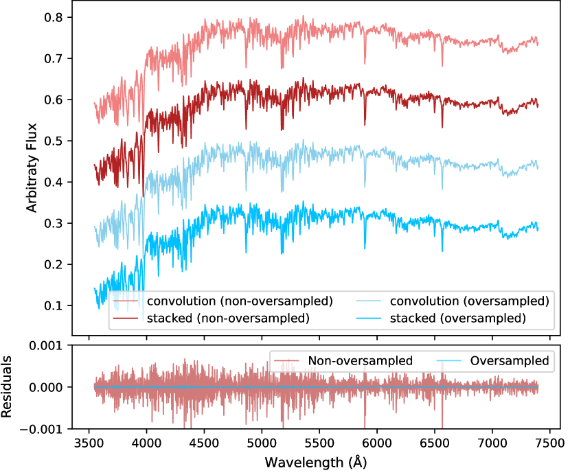
Figure 2: Comparison of the mock integrated spectrum generated by using the non-oversampled (in red and light-red) and the oversampled (in blue and light-blue) MILES templates. The light-color lines are spectra convolved by a Gaussian kernel with given $(\mu,\sigma)$, which is the way of pPXF measuring kinematics. The dark-color lines are spectra stacked by 2000 shifted spectrum with different line-of-sight velocities which follow a Gaussian distribution with the same $(\mu,\sigma)$, which is the manner of GalCraft. The bottom panel shows residuals of convolved and stacked spectra. By calculating the residuals of these two lines (shown in the residual panel), we find that oversampling can reduce the deviation between the convolved and stacked spectrum significantly by a factor of $\sim 25$.

Other than the above procedures, there are a few points that need to be clarified to the users as follows:

• The original mock stellar catalog in step (i) should have two coordinate systems, Cartesian coordinates $(x,y,z)$ and Galactic coordinates $(l,b)$, where $(l,b)$ are overlapped with $(y,z)$, respectively. Therefore, by adjusting $(\theta_{zx},\theta_{yz})$, users can change the inclination of the Galaxy at any angle. This is convenient when compared with real observations.

• The oversampling in step (v) has two purposes: one is to ensure the validity of degrading - when degrading the SSP templates from the original spectral resolution to instrumental resolution (e.g., from MILES to MUSE), the $\sigma$ of the Gaussian kernel to be convolved with the templates will be smaller than wavelength interval $\Delta\lambda$ without oversampling. In this case, the kernel function array becomes invalid with only one element having a value of 1, and the rest having values of 0. Then the degraded spectrum will be still in its original resolution. Another reason is to minimize the sampling error when stacking the spectrum with different line-of-sight velocities. Fig. 2 shows an example mock integrated spectrum generated by using the non-oversampled (in red and light-red) and oversampled (in blue and light-blue) MILES SSP templates. The light-color lines are the spectra convolved with a Gaussian kernel by the given mean velocity and dispersion $(\mu,\sigma)$, which is the manner of pPXF during the kinematics measurements. The dark-color lines are stacked from 2000 spectra shifted by Gaussian distributed line-of-sight velocities using the same $(\mu,\sigma)$, which is the manner of GalCraft. By calculating the residuals of these two lines (shown in the residual panel), we find that oversampling can reduce the deviation between the convolved and stacked spectrum significantly by a factor of $\sim 25$.

• This package can select a portion of particles within the field of view (FoV) of the user-defined instrument to generate the data cube, rather than take a whole catalog into account. It helps to mimic a more realistic IFS observation and reduces computational expenses.

• GalCraft can be executed in the batch mode where users can provide a list of cubes with the central coordinates in $(l,b)$ or $(ra,dec)$, and all the cubes can be automatically generated in one execution;

• Other than the data cube FITS file, this package also generates some by-products (optional), such as mass/light-fraction distributions and number of particles array for each spatial bin, mass/light-weighted $[\mathrm{M/H}]$, $[\mathrm{\alpha/Fe}]$, age and kinematic distribution maps in the Galactic coordinates, etc. These by-products are obtained from E-Galaxia particles’ properties and can be used to calculate the expected true answers that pPXF should recover from spectrum fitting. This will be described in detail in Section 3.

2.4 Estimate the Sampling Error

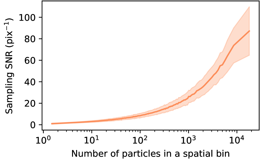
Figure 3: The sampling signal-to-noise ratio (SNR) of an integrated spectrum as a function of the number of particles of a spatial bin. The shaded region is the standard deviation of sampling SNRs for spaxels in the same number of particle bin. This is calculated by using original and bootstrapped mock data cubes later in Section 3.1. This figure provides an estimation of spectral sampling noise due to the limited number of particles.

Compared to the real catalogs of the Milky Way (e.g. Gaia), one shortcoming of the E-Galaxia mock stellar catalog is the limited number of particles. Although there are $10\sim 100$ times more particles $(10^{8})$ in the mock stellar catalog compared to MWAs in N-body/hydrodynamical simulations, it is inevitable that some spatial bins contain too few particles for robust measurements of their properties. Even for spaxels or Voronoi bins containing more than $\sim 10^{4}$ particles, the spectral noise due to finite star particles is still non-negligible. We call this type of spectral noise “sampling error" $(e_{f,S})$. One way to reduce sampling error is to generate more particles from E-Galaxia. However, this will increase the computational expenses and memory usage of GalCraft significantly, and exceed most of the HPCs’ limitation ($\sim 22$ GB for a catalog containing $10^{8}$ particles, hence $\sim 220$ GB for $10^{9}$ particles). Therefore, when mocking IFS observations, one has to ensure that for each integrated spectrum, the sampling error is smaller than the observational flux error ($e_{f,M}$ assuming MUSE observations) due to instrument conditions and exposure time. In this way, it is safe to apply the data reduction pipeline on this mock data cube and allow pPXF to derive mathematically reasonable results. This is particularly important in kinematics because the LOSVD effect in GalCraft integrated spectra is implemented by stacking individual spectra of particles with each shifted by its own $V_{\rm LOS}$. But pPXF employs the Gauss-Hermite function to convolve with SSP templates and determines the kinematics moments. In Section 3.2, we will provide a detailed example of how to deal with the sampling error for each Voronoi bin.

To estimate the sampling error, the GalCraft code provides an option to apply bootstrapping. First, it randomly re-selects particles from the original E-Galaxia catalog and generates a bootstrapped catalog with the same particle number ($N_{p}$). Then, GalCraft uses this catalog to generate bootstrapped data cubes. Repeating the above procedures a certain number of times, then the sampling error for each spaxel can be represented by the standard deviation of these bootstrapped fluxes. This sampling flux error will be used as the lower limit of the acceptable Gaussian noise when mimicking the real observations and obtaining the final integrated spectra of Voronoi bins. Fig. 3 illustrates how the sampling $\rm{SNR}$ (flux divided by sampling noise) varies as a function of the number of particles in a spatial bin. The shaded region is the standard deviation of sampling SNRs for spaxels having the same number of particles. We obtain this figure by using the original and bootstrapped mock data cubes later in Section 3.1. It can be seen that a spatial bin with $\sim 10^{3}$ particles can generate a spectrum with sampling $\rm{SNR}\sim 25$ $\text{pix}^{-1}$, and a spatial bin with $\sim 10^{4}$ particles can generate a spectrum with sampling $\rm{SNR}\sim 80$ $\text{pix}^{-1}$.

2.5 Computational Expenses and Multiprocessing Strategy

The execution time of GalCraft to generate mock data cubes depends mostly on the number of particles included in the instrument FoV and the spectral interpolation method. In general, the execution time is proportional to the number of particles used, and the “nearest" interpolation is three times faster than the “linear" interpolation. In this code, we apply python-multiprocessing techniques to speed up the computing. For a typical MUSE FoV containing $6\times 10^{6}$ particles, the execution time spent with a 24-core CPU (2.50GHz) is $\sim 1.4$ hour. Based on this, the users can roughly estimate the execution time they will spend. If taking into account the bootstrapped cubes, the total execution time will be multiplied by the number of bootstrapping times plus 1. Therefore, it is highly recommended to run it on high-performance computers (HPC) or a Cluster where these 21 jobs can be executed simultaneously.

3 Recovery of the Galaxy Chemodynamical Properties

In this section, we test the ability of pPXF to recover galaxy properties by applying it to mock cubes generated using GalCraft. We measure kinematics ($V_{\rm LOS}$, $\sigma$, $h_{3}$, $h_{4}$), stellar population parameters (age, $[\mathrm{M/H}]$, $[\mathrm{\alpha/Fe}]$) and mass fraction distributions of different structural components. The analysis is performed in the same way as extra-galactic studies. Then we compare the results with the input true values that are obtained by stellar parameters in E-Galaxia catalog. This test allows us to access the consistency of parameters measured via broadly applied software in other studies (e.g. Pinna et al. 2019a, b; Scott et al. 2021; Martig et al. 2021), which was not possible previously as the true values of external galaxies are unknown. Furthermore, it also provides standard references for the future to better understand extra-galactic results (e.g., gradient, flaring) by distinguishing real distributions from artificial effects due to the measuring method (e.g., pPXF), projected view, and integrated light.

3.1 Mock Cube Generation for MUSE Instrument

We generate a mock MUSE observation by GalCraft, using the E-Galaxia catalog that contains $10^{8}$ particles. We removed particles with stellar age less than 0.25 Gyr because their position and kinematics are erroneous in the current version of E-Galaxia, and we confirmed that removing these particles does not affect our conclusions. The mock MW catalog is assumed to have a distance of $26.5$ Mpc and inclination of $86^{\circ}$ to the observer. The selected distance and inclination are the same as the projection of NGC 5746, which was observed by MUSE and has comprehensive analysis in Martig et al. 2021 (hereafter M21). We use MILES $\alpha$-variable SSP templates (Vazdekis et al., 2015) with the BaSTI stellar isochrones (Pietrinferni et al., 2004) and Kroupa Universal IMF (Kroupa, 2001). The templates have 53 bins in age, 12 bins in $[\mathrm{M/H}]$ and 2 bins in $[\mathrm{\alpha/Fe}]$ and we apply a “linear" interpolation to assign each particle a spectrum based on its age, $[\mathrm{M/H}]$ and $[\mathrm{\alpha/Fe}]$, and then degrade the stacked spectra to MUSE spectral resolution ($\mathrm{FWHM}\sim 2.65\Angstrom$). Following procedures in Section 2.3, we obtain two mock cubes focusing on the central $(N_{p}=61575676)$ and the disk $(N_{p}=7379847)$ regions, as shown in Fig. 4. This observation strategy is also the same as NGC 5746 in M21. The total execution time spent by GalCraft on a 24-core CPU for these two cubes is $\sim 14.5$ hours. We also generate $2\times 20$ bootstrapped cubes and use 16% and 84% percentiles to calculate the sampling error of each spaxel. We do not apply extinction in these cubes because here we only focus on the pPXF recovery ability. Adding extinction would blend all the effects and make it difficult to differentiate their individual impacts. Therefore, we reserve this topic for future studies.

Figure 4: Two mock data cube positions (in purple) relative to the number distribution of particles in E-Galaxia mock stellar catalog. The model was set with a distance of 26.5 Mpc and inclination of $86^{\circ}$. This observation strategy is the same as the MUSE observation on NGC 5746 by Martig et al. 2021.

The next procedure is to add Gaussian flux error to the spectra. We first derive the MUSE flux error $(e_{f,M})$ of the mock cubes. The flux error depends on many aspects but can be classified into two main categories: the observation conditions (seeing, air-mass, exposure time, etc.) and the instrumental properties (telescope aperture, system efficiency, dark current, read-out noise, etc). For simplicity, we ignore the sky conditions, dark current, and read-out noise which only contribute a few percent to total received photons, and assume the MUSE SNR and received photons are defined by

$$\begin{split}&\mathrm{SNR}=\frac{f}{e_{f,M}}=\sqrt{N},\\ &N=aft,\end{split}$$ (1)

where $f$ is the flux of the target; $e_{f,M}$ is the MUSE flux error; $N$ is the received number of photons; $t$ is the exposure time; $a$ is an overall reaction of sky transmission, efficiency and telescope aperture. Therefore, $a$ should be only dependent on wavelength for the same instrument. By substituting the above equations, the parameter $a$ can be calculated using $f$, $e_{f,M}$ and $t$ from an observation by

$$a=\frac{f}{e^{2}_{f,M}\times t}.$$ (2)

In this work, we take all the bulge and disk observations of NGC 5746 from M21 and fit equation 3 as a function of wavelength $(\lambda)$ using a 4-degree polynomial, which is described by

$$\begin{split}a(\lambda)&=4.34274826^{-18}\lambda^{4}-1.43263443^{-13}\lambda^{3}+1.61141240^{-9}\lambda^{2}\\ &-7.29164505^{-6}\lambda+1.17213217^{-2},\end{split}$$ (3)

where $a(\lambda)$ is in the unit of $1/10^{-20}~{}\rm{erg}~{}\rm{cm}^{-2}~{}\mbox{\AA}^{-1}$. Next, we set the bulge and disk mock cubes to have an exposure time of 1729.39 s and 6221.84 s, respectively, and use the equation 2 and 3 to estimate the flux error $e_{f,M}$ of each spaxel. Then we use this error to add Gaussian noise to all the spaxels. Finally, the two mock cubes are stitched together.

3.2 Extracting Galaxy Properties

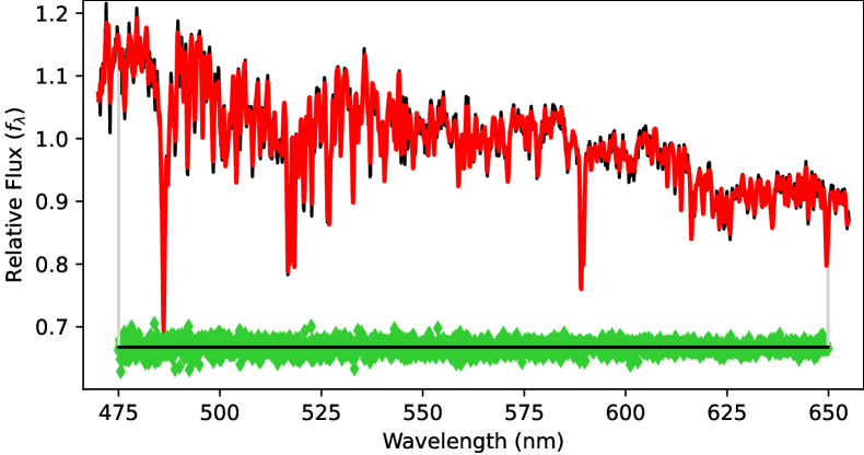
Figure 5: A spectral fit example of a Voronoi bin by pPXF in Section 3.2. The “observed" spectrum is in black while the best-fit spectrum is in red. Residuals are in green. The fitting area is within the grey lines on both sides.

We apply the GIST pipeline (Bittner et al., 2019) on the stitched mock cube to measure the kinematics and stellar population parameters. The GIST pipeline combines all the tools needed to process the data and the user can obtain final results in a single execution. Here we use a modified version to implement some functionalities that the current public version (v3.1.0) does not have but are needed in this work. A detailed list of added features is given in Appendix A.

We run the GIST pipeline in the following steps: First, we apply the Voronoi tessellation software (Cappellari & Copin, 2003) to spatially re-bin the mock cube and increase the SNR to 80 $\text{pix}^{-1}$, which results in 1477 Voronoi bins. Most of the Voronoi bins contain $N_{p}>10^{4}$. For the other Voronoi bins, $N_{p}$ is also very close to this number. To ensure the sampling noise $e_{f,S}$ is less than the MUSE flux error $e_{f,M}$, we apply the same Voronoi binning arrangement to all 20 bootstrapped cubes. Then we calculate the sampling noise $e_{f,S}$ of each Voronoi by taking half of the difference between the 16th and 84th percentiles of its 20 bootstrapped integrated spectra. We confirm that on average $e_{f,M}>e_{f,S}$ applies for all the Voronoi bins.

Next, we apply the full-spectrum fitting method pPXF (Cappellari, 2017) to measure the stellar kinematics of each Voronoi bin. Here we use the same MILES $\alpha$-variable templates (Vazdekis et al., 2015) as when we generated the mock cubes and degraded them to the same MUSE spectral resolution. Since there is no emission line or atmosphere effect, we use a wide wavelength range of $(4750,6550)\Angstrom$ to fit with the Voronoi binned spectra and remove the first and last $75\Angstrom$ to avoid effects caused by spectral oversampling, rebinning and Doppler shifting, etc. During the fitting, the MILES templates are convolved with a line-of-sight velocity distribution (LOSVD) described by a Gauss-Hermite equation to match the Voronoi binned spectrum. We parameterize the LOSVD using four moments, which are mean line-of-sight velocity $V_{\rm LOS}$, line-of-sight velocity dispersion $\sigma$, and the third- and fourth-order moments $h_{3}$, $h_{4}$. No regularization is applied in this process, and we include a fourth-order multiplicative Legendre polynomial.

After measuring kinematics, we employ pPXF again to obtain the stellar population parameters for each Voronoi bin. We choose the same templates, spectral resolution, and fitting wavelength range as the previous step. Each template is normalized to one solar mass ($\mathrm{M}_{{\odot}}$). We use the LOSVDs ($V_{\rm LOS}$, $\sigma$, $h_{3}$, $h_{4}$) measured in the last step as input, and fix them during the fitting to obtain the weight of each template. The best-fit spectrum is the weighted sum of all the templates. For the initial fitting, we set no regularization to obtain the initial $\chi^{2}$. Then we follow the approach in McDermid et al. (2015) and iterate the fitting by increasing $R$ until $\chi^{2}$ is increased by $\Delta\chi^{2}=\sqrt{2N}$, where $N$ is the number of wavelength pixels considered for the fit. This iteration process allows us to obtain the smoothest solution that is still compatible with the data within $1\sigma$ level. At this stage, we note $R$ reaches the maximum regularization $R_{max}$. Next, we choose $R=5$ which is between 0 and $R_{max}$ $(30\sim 100)$ to keep smooth solutions while still allowing for a variation on short timescales of the star formation, which will disappear if $R$ is too large (see similar discussions in Pinna et al. 2019a and M21). Fig. 5 is an example of the fitting results for the spectrum of one Voronoi bin. Finally, using the weights, we can calculate mass-weighted age, $[\mathrm{M/H}]$, $[\mathrm{\alpha/Fe}]$, and mass fraction distributions.

In addition, we also apply the LS module in the GIST pipeline to compute line-strength indices of each Voronoi bin spectrum in the LIS system (Vazdekis et al., 2010) choosing the definitions provided at a spectral resolution of 8.4 Å. This routine was presented by Kuntschner et al. (2006) and Martín-Navarro et al. (2018). Next, given the relationship between templates’ properties (age, $[\mathrm{M/H}]$, $[\mathrm{\alpha/Fe}]$) and line strengths, the measured line strengths can be matched to SSP-equivalent parameters by using the MCMC implementation from the package emcee (Foreman-Mackey et al., 2013). In this work, we follow M21 and use $\mathrm{H}\beta_{\mathrm{o}}$ as an age indicator and Fe5015, Fe5270 and Fe5335, and $\mathrm{Mg}b$ to trace metallicity and $[\mathrm{\alpha/Fe}]$. The Monte-Carlo simulation is run 15 times and each one uses 100 walkers and 1000 iterations to obtain uncertainties.

After measuring all the parameters, in the next sub-sections, we compare the kinematics, mass-weighted stellar population parameters, and mass fraction distributions of the mock cube with the true values to verify the recovery ability of pPXF.

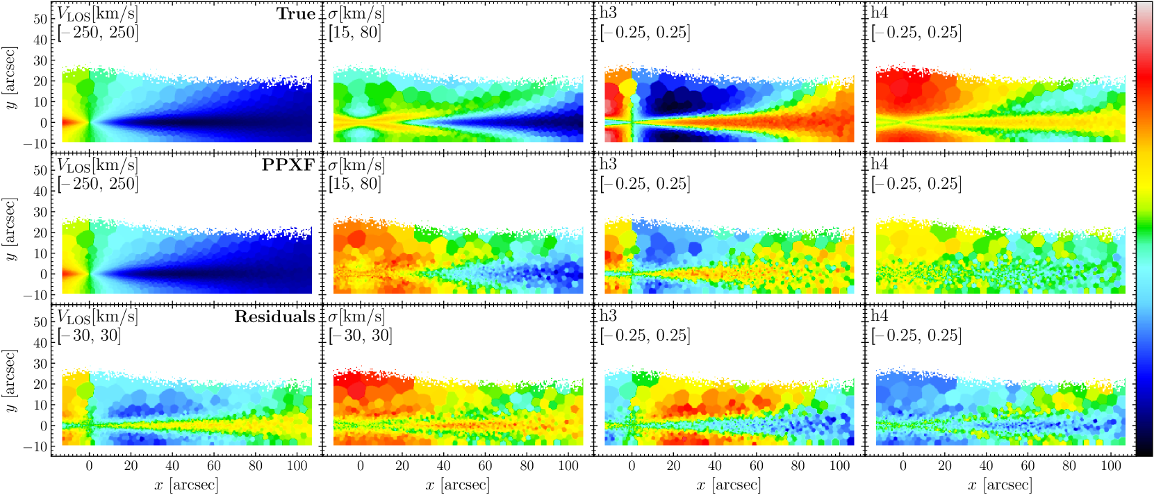
Figure 6: Stellar kinematic maps ($V_{\rm LOS}$, $\sigma$, $h_{3}$, $h_{4}$) of the mock MUSE cube generated in Section 3.1. The scale of the color bar is given in the second row of the upper left corner for each panel. Top row: True values calculated by fitting a Gauss-Hermite function with particles’ velocity distribution weighted by their total flux in pPXF fitted wavelength region for each Voronoi bin. Middle row: Results from pPXF. Bottom row: Residuals of the pPXF results and the true values for each moment. The residual panels indicate results from pPXF have systematic offsets compared to true values.

3.3 Kinematic Maps

Fig. 6 shows the kinematics maps in four moments ($V_{\rm LOS}$, $\sigma$, $h_{3}$, $h_{4}$) of the mock MUSE cubes. The scale of the color bar is given in the second row of the upper left corner of each panel. We calculate the true values in the first with the following procedures: First, for each Voronoi bin, we calculate the total flux of each particle in the pPXF fitted wavelength region. Then we plot flux-weighted $V_{\rm LOS}$ histogram distribution using all the particles included in this bin. Next, we fit this histogram with a Gauss-Hermite function and obtain four best-fit moments ($V_{\rm LOS}$, $\sigma$, $h_{3}$, $h_{4}$). This method is consistent with the definition of light-weighted kinematics which pPXF is expected to recover during the fitting process. The middle row is the results from pPXF and the bottom rows are residuals of the pPXF results and the true values.

In this figure, the kinematic moments obtained by pPXF have the same trend compared to the true values. Both show two kinematically distinct components: one is aligned to $y\sim 0$ and the thickness increases with $x$, which has larger absolute $V_{\rm LOS}$ and $h_{3}$, and smaller $\sigma$; the other is in a similar projected radius but vertically higher and thicker, and it has smaller absolute $V_{\rm LOS}$ and $h_{3}$, but larger $\sigma$. An anti-correlation of $h_{3}$ with $V_{\rm LOS}$ which are usually associated with disk-like components (e.g. Krajnović et al. 2008; Guérou et al. 2016; van de Sande et al. 2017) is seen and are similar to MUSE edge-on galaxies studies of Pinna et al. (2019a, b) and M21. In Section 3.6, we will define these two components as thin and thick disks.

However, in the residual panels, all these four moments show systematic offsets. Compared to the true values, $V_{\rm LOS}$ from pPXF is around $17$ km s^-1 lower above and below the very thin mid-plane ($y\sim 0$) and shows an overestimation around $x\sim[10,30]$ arcsec. Around the galaxy center, the residual of $V_{\rm LOS}$ also shows a continuous decrease from negative to positive $x$; $\sigma$ is generally overestimated everywhere in the galaxy with few light blue residuals. $h_{3}$ is overestimated in regions of $x\sim[20,60]$ arcsec and $y\sim[10,25]$ arcsec and underestimated in the outer region of $x\sim[60,110]$ arcsec; $h_{4}$ from pPXF has no significant structures like $\sigma$ and $h_{3}$ maps, which is also seen in real galaxies results (e.g., Pinna et al. 2019a, b and M21), but the true $h_{4}$ map clearly shows kinematic differences. The clear structures in these residual panels indicate that it is not because of the fitting uncertainties. We will discuss this issue in detail and provide our investigations in Section 4.1.

3.4 Mass-weighted Stellar Population Parameter Maps

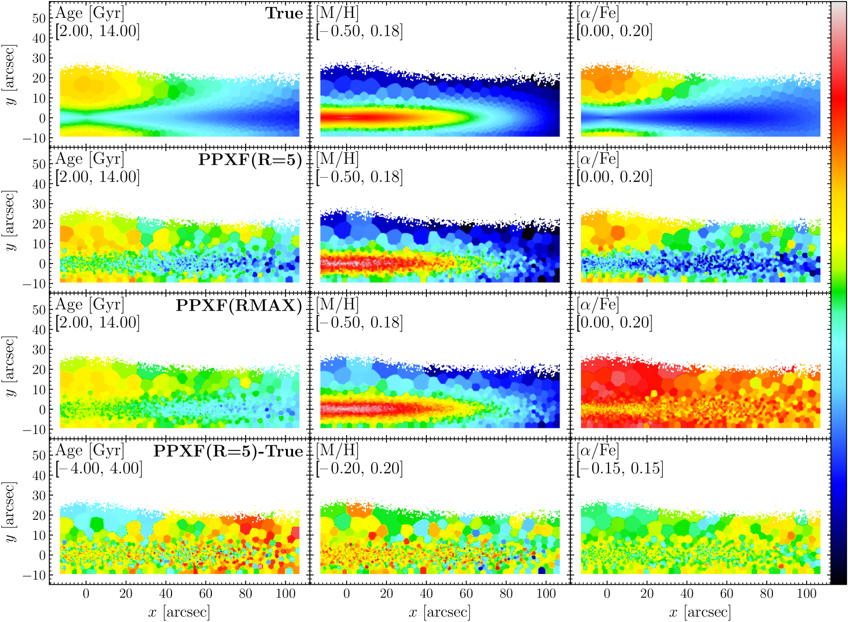
Figure 7: Stellar population maps (age, $[\mathrm{M/H}]$ and $[\mathrm{\alpha/Fe}]$) of the mock MUSE cube generated in Section 3.1. The scale of the color bar is given in the second row of the upper left corner for each panel. First row: True values calculated by the mass-weighted average of particles’ age, $[\mathrm{M/H}]$ and $[\mathrm{\alpha/Fe}]$ for each Voronoi bin. Second row: Results from pPXF via full-spectrum fitting with regularization $R=5$. Third row: Results from pPXF with $R=R_{max}$, calculated using strategies of McDermid et al. 2015. Last row: Residuals of pPXF results with $R=5$ and the true values. This figure indicates that pPXF results with proper regularization can identify different galaxy components by their stellar population parameters, which are consistent with true values. Applying $R=R_{max}$ during the fitting can smooth the distribution and make different $[\mathrm{\alpha/Fe}]$ components indistinguishable. According to residuals, stellar age in the outer region and $[\mathrm{M/H}]$ in the center region are overestimated.

Fig. 7 shows the mass-weighted age, $[\mathrm{M/H}]$ and $[\mathrm{\alpha/Fe}]$ maps of the mock MUSE cubes. The first row is the true values by calculating the particles’ median age, $[\mathrm{M/H}]$ and $[\mathrm{\alpha/Fe}]$ for each Voronoi bin, which are equivalent to mass-weighted values since each particle is weighted as $1$ $\mathrm{M}_{{\odot}}$. The second row is the results from pPXF with regularization $R=5$. The third row is the results from pPXF with $R=R_{max}$. The last row shows the residuals of the pPXF results with $R=5$ and the true values. The overall distributions of these three parameters obtained by pPXF are very close to the true values. This confirms the reliability of using pPXF to measure the weighted chemical compositions. Especially, the $[\mathrm{\alpha/Fe}]$ map from pPXF with $R=5$ indicates the capability of pPXF to identify $[\mathrm{\alpha/Fe}]$-rich and $[\mathrm{\alpha/Fe}]$-poor populations in the thick and thin disk, respectively, even though only two $[\mathrm{\alpha/Fe}]$ bins are available. The residuals of $[\mathrm{\alpha/Fe}]$ from pPXF with $R=5$ and the true values are flat and no systematic pattern is found.

However, minor offsets appear in age and $[\mathrm{M/H}]$ residual panels: age from pPXF is mostly overestimated in the outer regions while $[\mathrm{M/H}]$ is overestimated in the inner center regions. This means the age gradient from pPXF is underestimated but the $[\mathrm{M/H}]$ gradient is overestimated. In addition, the $[\mathrm{\alpha/Fe}]$ distribution from pPXF results with $R=R_{max}$ is almost uniformly high and much larger than the true values for all the Voronoi bins. This is because when $R$ is very large, the pPXF algorithm forces the result to have very smooth template weights in three parameter dimensions (age, $[\mathrm{M/H}]$, $[\mathrm{\alpha/Fe}]$). Since there are only two $[\mathrm{\alpha/Fe}]$ grids, regularization will force them to have similar weights to achieve smoothness and does not permit large deviations (e.g., more than 0.1 dex). Therefore, it will be challenging to identify $[\mathrm{\alpha/Fe}]$ bimodality. Results from pPXF with $R=R_{max}$ also show much underestimation for age gradients than results with $R=5$. The age and $[\mathrm{M/H}]$ gradients are essential properties to help understand the star formation and chemical enrichment processes. Therefore, a wrong choice of regularization will then easily lead to wrong conclusions. We will explore these offsets in more detail in Section 3.6 using mass fraction distributions and the effect of regularization in Section 4.3.

3.5 SSP-equivalent Maps from Line-Strength Indices

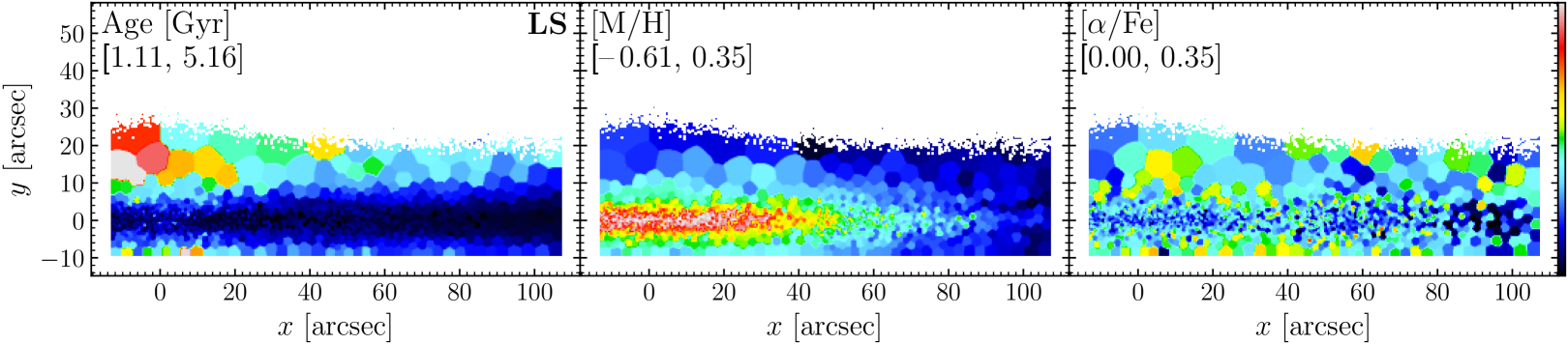
Figure 8: SSP-equivalent age, $[\mathrm{M/H}]$ and $[\mathrm{\alpha/Fe}]$ maps of the mock MUSE cube generated in Section 3.1. The parameters are measured by line-strength indices. The scale of the color bar is given in the second row of the upper left corner for each panel. Similar to Fig. 7, galaxy components with different ages, $[\mathrm{M/H}]$, and $[\mathrm{\alpha/Fe}]$ can be identified. However, the parameter ranges differ from pPXF results and the true values.

Fig. 8 shows the SSP-equivalent age, $[\mathrm{M/H}]$ and $[\mathrm{\alpha/Fe}]$ maps of the mock MUSE cubes measured by line-strength indices. This figure shows that the main structures we derived from pPXF are also recovered by the line-strength analysis with consistent trends. In the age panel, young populations are closer to the mid-plane, and old populations are further to the mid-plane or above/below the central region. In the $[\mathrm{M/H}]$ panel, we see the metallicity gradient from the inner center to the outer Galaxy. In the $[\mathrm{\alpha/Fe}]$ panel, we see the $\alpha$-rich bins in the center and $\alpha$-poor bins in the outer region. The main difference compared with pPXF results is that the age panel shows a very low range of $[1\sim 5]$ Gyr. This is also seen in M21 (Fig. B1) and because of the Balmer line indices being dominated by young stars. Therefore, the SSP-equivalent ages only reflect the fraction of stars formed within the past Gyr (Serra & Trager, 2007; Trager & Somerville, 2009). The SSP-equivalent $[\mathrm{M/H}]$ and $[\mathrm{\alpha/Fe}]$ range are much closer compared to pPXF results because young populations do not contribute much to the metal lines, which is also indicated in M21. This figure confirms that both line-strength indices and pPXF analysis can identify $\alpha$-rich (thick disk) and $\alpha$-poor (thin disk) populations.

3.6 Mass Fraction Distributions of Different Galaxy Components

Figure 9: Demonstration of the projected thin disk (blue), thick disk (red), upper central (purple), and inner central (orange) regions on top of a grey-scale image of the mock data cube generated in Section 3.1. These regions will be used to study the mass fraction distribution of different galaxy components later.

In addition to calculating the mass-weighted parameters, we can also study the mass fraction distribution of stellar populations along the age and $[\mathrm{M/H}]$ space. This is done by using weights of templates from pPXF. Because the flux of each template is normalized to 1 $\mathrm{M}_{{\odot}}$, the weights array from pPXF outputs in our tests are equivalent to stellar population mass fractions. Therefore, we can study the mass distribution of any component of the Galaxy. M21 employed multiple components morphological fitting to a Spitzer 3.6 micron image to obtain regions dominated by the boxy/peanut bulge, nuclear disk, and thin and thick disks. In Fig. 9, we artificially select similar regions based on the locations $(x,y)$, kinematics, and stellar population parameters of different components of M21, and name them “upper central", “inner central", “thin disk" and “thick disk", as shown in different colors. We call them “upper central" and “inner central" because there is no boxy/peanut bulge and nuclear disk in the GCE of S21. Note these component definitions are purely following those in M21 to mock their data analysis. In reality, radial scale lengths of the thin disk $(R^{t})$ and thick disk $(R^{T})$ in NGC 5746 and the MW are very different ($R^{t}_{\mathrm{MW}}=2.6\pm 0.5$ kpc and $R^{T}_{\mathrm{MW}}=2.0\pm 0.2$ kpc from Bland-Hawthorn & Gerhard 2016; $R^{t}_{\mathrm{NGC~{}5746}}=6.1$ kpc and $R^{T}_{\mathrm{NGC~{}5746}}=8.2$ kpc from M21). For each component, the mass weights of all the Voronoi bins are combined to represent its mass fraction distribution.

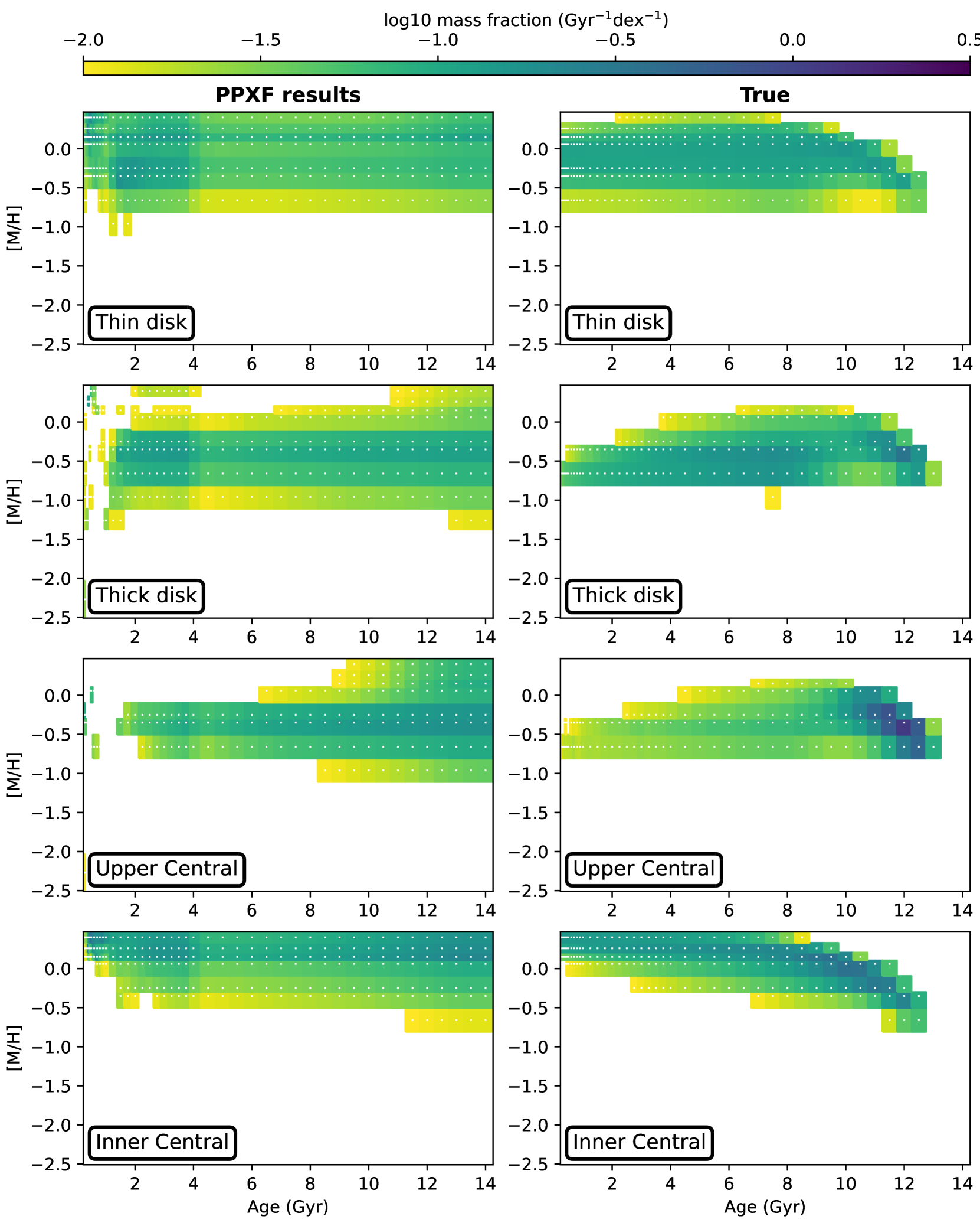
Figure 10: Mass fraction distributions of the thin disk, thick disk, inner central, and upper central of the mock data cube generated in Section 3.1. Mass fraction weights are normalized to one for each panel. Left-hand column: Results from pPXF with $R=5$. Right-hand column: True values calculated using particles’ properties in mock E-Galaxia catalog. The color bar is shown on the top. We only plot the weights above 0.001 $\text{Gyr}^{-1}\text{dex}^{-1}$. This figure indicates the broad trends of results from pPXF are consistent with the true values. However, there is an overdensity in $2\sim 4$ Gyr, and populations around 12 Gyr are smoothed towards older, more metal-rich regions, which are not seen in the true values. We present detailed discussions about this figure in Section 4.2.

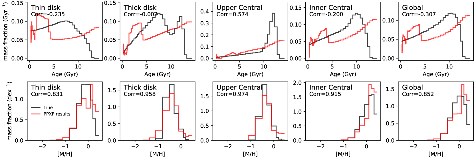
Figure 11: Age distribution (top row) and $[\mathrm{M/H}]$ distribution (bottom row) of the thin disk, thick disk, inner central, and upper central of the mock data cube generated in Section 3.1. These panels are obtained by integrating the mass fraction distributions in Fig. 10 along $[\mathrm{M/H}]$ and age axis, respectively. Red lines are results from pPXF with $R=5$. Black lines are the true values calculated using particles’ properties in the mock E-Galaxia catalog. The correlation coefficient of these two lines is texted in the left top corner. Especially, the correlation of age distributions is calculated after evenly re-binning the age grid into linear space. The overall trends from pPXF are consistent with the true values for $[\mathrm{M/H}]$. However, same as Fig. 10, the mass fraction is overestimated in $2\sim 4$ Gyr and $12\sim 14$ Gyr and underestimated in $5\sim 12$ Gyr for all the components, and the coefficients indicate inconsistency for age distributions. We also find peaky features in regions less than 1 Gyr. The mass weights of the most metal-rich bin are overestimated for all the components.

Fig. 10 shows the mass fraction distributions of these four components, respectively. The total weights are normalized to one for each panel. The left column is the results from pPXF with $R=5$, and the right column shows the true values calculated using particles’ properties in the mock stellar catalog. We only plot the weights above 0.001 $\text{Gyr}^{-1}\text{dex}^{-1}$. For the thin disk, true values indicate a rapid metallicity enrichment history $\sim 10$ Gyr ago, and it slowly increases later on. While from pPXF results, mass fraction weights are dominated by two regions, which are relatively young ($2\sim 4$ Gyr) and old ($12\sim 14$ Gyr) stellar populations and the metallicity enrichment trend is indistinguishable. The same features are also seen in other Galaxy components. For the overdensity region of $2\sim 4$ Gyr, we think this is due to the decrease in template age bin size from old to young population. For the region of $12\sim 14$ Gyr, we think this is because at the level of $\rm{SNR}\sim 80$ $\text{pix}^{-1}$, the differences between nearby old, metal-rich templates are smaller than the Gaussian noise added on the spectra, causing the degeneracy in this parameter region. More details will be discussed in Section 4.2. For the thick disk, true values also show the metallicity enrichment trend, but the populations born less than $1$ Gyr are more metal-poor than the thin disk; This is due to the geometrical definition of the thick disk, which contains younger and relatively more metal-poor stars that are flared in the outer disk ($x\sim[60,80]$ arcsec). Given that NGC 5746 from M21 is four times more massive than the MW, it has a larger scale length and the definition of its thick disk might not apply to the MW. Another reason is due to the projection effect, where young stars flared in the outer disk could appear at the front and back of the line of sight in the region of $x\sim[30,60]$ arcsec. The upper central shows a similar trend with the thick disk but is more dominated in the old populations, but this domination is smoothed out in the pPXF results; For the inner central, true values are showing a clearer chemical enrichment trend and there is no new population born with $[\mathrm{M/H}]{}<-0.2$ dex in the young region, while the pPXF results show again two regions with higher mass fractions, one at $\sim 2$ Gyr and the other at $12\sim 14$ Gyr. Therefore, except for the overestimation in the young and old regions, the mass fraction distributions of pPXF are generally in agreement with true values.

In Fig. 11, we integrate the mass fraction distributions in Fig. 10 along the two axes and derive age and $[\mathrm{M/H}]$ distributions for each component. The top panels are mass distributions as a function of age which is the definition of star formation history or star formation rate, and the bottom panels are as a function of $[\mathrm{M/H}]$. Results from pPXF are in red lines and the true values are in black lines. For each panel, we calculate the correlation between these two lines to quantify their similarity. For the age distributions, we find the same as in Fig. 10. Compared to the true values, the pPXF results of all the components demonstrate an overestimation of weights in the ranges of $2\sim 4$ Gyr and $12\sim 14$ Gyr and underestimation in the range of $4\sim 11$ Gyr. The underestimated regions seem to compensate for the overestimated regions. And the thin disk, inner central, and global panels show a peaky feature with age $<1$ Gyr. For the $[\mathrm{M/H}]$ distributions, pPXF results are consistent with true values for most regions, as indicated by the correlation coefficients. However, weights in the metal-rich region are overestimated by pPXF. Other than that, the overall trend of results from pPXF is consistent with true values.

In conclusion, we find that pPXF can recover the broad trends of 2-D mass fraction distributions for different components, but with overestimation in $2\sim 4$ Gyr, $12\sim 14$ Gyr and most metal-rich regions. When integrating into 1-D age and metallicity distributions, these inconsistencies are significant. According to correlation coefficients, $[\mathrm{M/H}]$ distributions are more consistent with the true values than age distributions. We will investigate the reasons for such differences in detail in Section 4.2.

3.7 Distributions of $[\mathrm{\alpha/Fe}]$-$[\mathrm{M/H}]$ along Different Galaxy Locations $(R,z)$

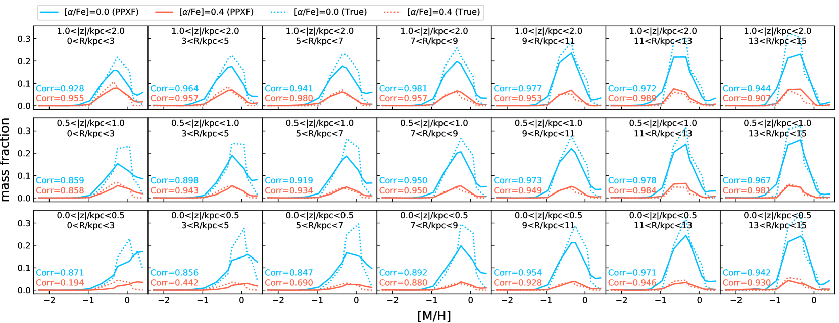
Figure 12: $[\mathrm{M/H}]$ distributions for different $[\mathrm{\alpha/Fe}]$ components distributed along projected $R$ and $|z|$ of the mock cube generated in Section 3.1. For each panel, the total mass fractions of true (dotted lines) and pPXF (solid lines) are normalized to 1, respectively. Blue lines represent mass fraction distributions for $[\mathrm{\alpha/Fe}]$ $=0.0$ dex while red lines represent the component with $[\mathrm{\alpha/Fe}]$ $=0.4$ dex. Solid lines represent the results from pPXF and dotted lines are the true values. This figure is similar to the $[\mathrm{\alpha/Fe}]$-$[\mathrm{Fe/H}]$ distributions in Hayden et al. 2015 and Scott et al. 2021. The correlation coefficient of the dotted and solid lines are texted in the same color in the left bottom panel. For most of the panels, pPXF results are consistent with the true values. The discrepancy happens on the inner central and thin disk, where both lines show a mass fraction underestimation at $[\mathrm{M/H}]$ $\sim 0.0$ dex and overestimation at the most metal-rich regions.

According to S21, different radial migration and kinematic heating rates will cause different fractions of stars in the distinct $[\mathrm{\alpha/Fe}]$-rich and $[\mathrm{\alpha/Fe}]$-poor sequences. A recent study by Scott et al. (2021) derived this distribution from an external galaxy UGC 10738 using MILES $\alpha$-variable templates (Vazdekis et al., 2015) and concluded it has similar bimodality distributions to the MW. Since we know the true values from the mock stellar catalog particles, here we explore the recovery ability of pPXF on measuring the changes of this bimodality at different projected $R$ and $|z|$. Different from Scott et al. (2021) where they compared integrated values of UGC 10738 with individual stellar values of the MW, our integrated-to-integrated value comparison is more direct and there is no systematic bias due to different methodologies. This direct comparison also provides an example for future studies on comparing an integrated version of the MW $[\mathrm{\alpha/Fe}]$ bimodality with MW-like edge-on galaxies from MUSE observations (e.g., GECKOS survey van de Sande et al. 2023).

The results are shown in Fig. 12 where we separate different locations in the same way as Hayden et al. (2015). For each panel, the total mass fraction given by true (dotted lines) and pPXF (solid lines) is normalized to 1, respectively. Blue lines are mass fraction distributions for $[\mathrm{\alpha/Fe}]{}=0.0$ dex while red lines represent $[\mathrm{\alpha/Fe}]{}=0.4$ dex. The overall trends for $[\mathrm{\alpha/Fe}]$-rich and $[\mathrm{\alpha/Fe}]$-poor sequences from pPXF are consistent with the true values for most of the panels, which indicates both sequences are well recovered by pPXF, as also shown by correlation coefficients. However, there are some discrepancies such as in the inner regions ($R<5$ kpc) and thin disk ($|z|$<0.5 kpc), where pPXF show smoother metallicity distributions in both the blue and red lines compared to true values. In addition, the mass fraction is underestimated at $-1<[\mathrm{M/H}]<0.0$ dex and overestimated at the most metal-rich regions, which is also seen in metallicity distributions in Fig. 11. Because we do not see the tail at the most metal-rich regions in the true values for both $[\mathrm{\alpha/Fe}]$ sequences, this difference is more likely due to the degeneracy of metal-rich populations; these spectra are very similar which means that pPXF will obtain more uncertain results.

When comparing different $[\mathrm{\alpha/Fe}]$ sequences, the metallicity positions with the highest mass fraction are identical in both pPXF and true values. This differs from our understanding of $[\mathrm{\alpha/Fe}]$-$[\mathrm{M/H}]$ relation of the Milky Way. It is more likely due to the limited number of $[\mathrm{M/H}]$ and $[\mathrm{\alpha/Fe}]$ bins in MILES templates that cause the differences of metallicity distribution in different $[\mathrm{\alpha/Fe}]$ bins to be indistinguishable. Similar findings are also mentioned by Scott et al. (2021) when they analyzed the $[\mathrm{\alpha/Fe}]$-bimodality of UGC 10738. Therefore, we emphasize that more $[\mathrm{M/H}]$ and $[\mathrm{\alpha/Fe}]$ bins in the spectral templates are necessary to obtain more detailed distributions of this bimodality. It can help to make it more feasible to identify the effect of different radial migration and kinematic heating efficiency from the relative fractions of these two sequences when compared with other IFS observations.

4 Discussion

4.1 Systematic Offsets in the Kinematics Recovery

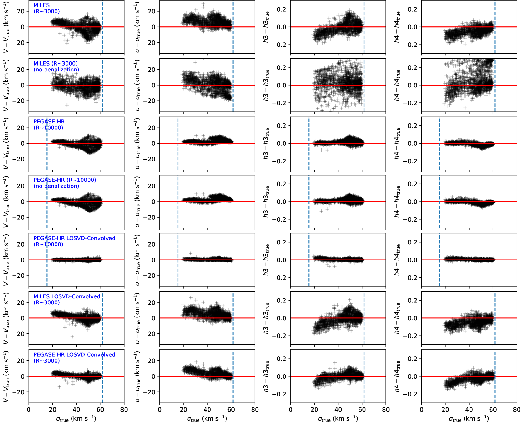
Figure 13: Stellar kinematics recovery of four Gauss-Hermite moments $\Delta$($V_{\rm LOS}$, $\sigma$, $h_{3}$, $h_{4}$) as a function of true velocity dispersion. Each data point represents a Voronoi bin. The red line represents zero to guide the eyes. The vertical dashed line indicates the instrumental dispersion $\sigma_{\rm inst}$. First row: Results from pPXF using MILES templates in MUSE spectral resolution ($\sigma_{\rm inst}$ $\sim 62$ km s^-1), same as the residual panels in Fig. 6. Second row: Similar to the first row but results are fitted by pPXF with no penalization on $h_{3}$ and $h_{4}$. Third row: Results from pPXF on a mock cube similar to Section 3 but generated and fitted using PEGASE-HR (Le Borgne et al., 2004) templates ($\sigma_{\rm inst}$ $\sim 15$ km s^-1). Fourth row: Similar to the third row but penalization was turned off during pPXF fitting. Fifth row: Similar to the second row but for LOSVD-Convolved mock cubes. Sixth row: Similar to the first row but for LOSVD-Convolved mock cubes. Seventh row: Similar to the fourth row but all the analysis is in MUSE resolution to eliminate the effects of different SSP templates. This figure indicates that both the spectral resolution and the relation between LOSVD and age, $[\mathrm{M/H}]$ affect the kinematics recovery.

In Fig. 6, we show the deviations between the kinematics map from pPXF and the true values. To better illustrate the offsets of each moment, we plot their residuals as a function of true velocity dispersion $\sigma_{\rm{true}}$ in Fig. 13, in which the y-axis value is calculated by pPXF fitted value subtracting the true value. Each data point represents one Voronoi bin. The blue dotted lines represent the instrumental dispersion ($\sigma_{\rm inst}$) in MUSE spectral resolution. We also plot the zero-line in red to guide the eyes. The first row demonstrates the results in Fig. 6, and it clearly shows the systematic offsets for each moment: $\Delta$$V_{\rm LOS}$ increases with $\sigma_{\rm{true}}$, and $\sigma$ is overestimated for most of the Voronoi bins; as for $h_{3}$ and $h_{4}$, the residuals have a slight positive slope with $\sigma_{\rm{true}}$.

From Fig. 6, we find that several Voronoi bins have large absolute $h_{3}$ and $h_{4}$ true values (e.g., central region and the thick disk). These higher-order moments are not well constrained when SNR is relatively low (Cappellari & Emsellem, 2004; Pinna et al., 2021). Therefore, pPXF with keyword bias will penalize them towards lower absolute values during the fitting to make the LOSVD towards a Gaussian. However, using different penalizations can result in different kinematic measurements (see full analysis using SAMI galaxies by van de Sande et al. 2017). In our case, when $h3$ and $h4$ are larger than 0.15/0.2 the Gauss-Hermite approximation no longer works well, so differences are expected. Therefore, we turn off the penalization of these higher-order moments and re-measure the kinematics, and show the results in the second row of Fig. 13. A spatially distributed map can also be seen in Fig. 20 of the Appendix B. After turning off penalization, both $h_{3}$ and $h_{4}$ from pPXF are visually closer to the true values in Fig. 20. However, the second row of Fig. 13 still shows similar trends of $V_{\rm LOS}$ and $\sigma$, and $h_{3}$ and $h_{4}$ are very scattered, which indicates penalization is not the cause of the systematic offsets.

Another possible reason causing the kinematic inconsistency could be the low spectral resolution of the MUSE instrument. As shown in the first row of Fig. 13, $\sigma_{\rm{true}}$ values for most of the Voronoi bins are smaller than the MUSE instrumental dispersion $\sigma_{\rm inst}$$\sim 62$ km s^-1. In this case, the recovery of kinematics will be uncertain. This has been pointed out in Fig. 3 of Cappellari (2017), and the only way to avoid it is to increase the instrumental spectral resolution. The explanation is when $\sigma$ $<$ $\sigma_{\rm inst}$, during pPXF fitting, the broadening of one sharp spectral feature is less than the distance to its nearby wavelength pixels In this case, the nearby wavelength pixels have minor changes and this brings difficulties for pPXF to measure $\sigma$ correctly, and $h_{3}$ and $h_{4}$ will go towards zero because there are also not enough pixels to identify the skewness.

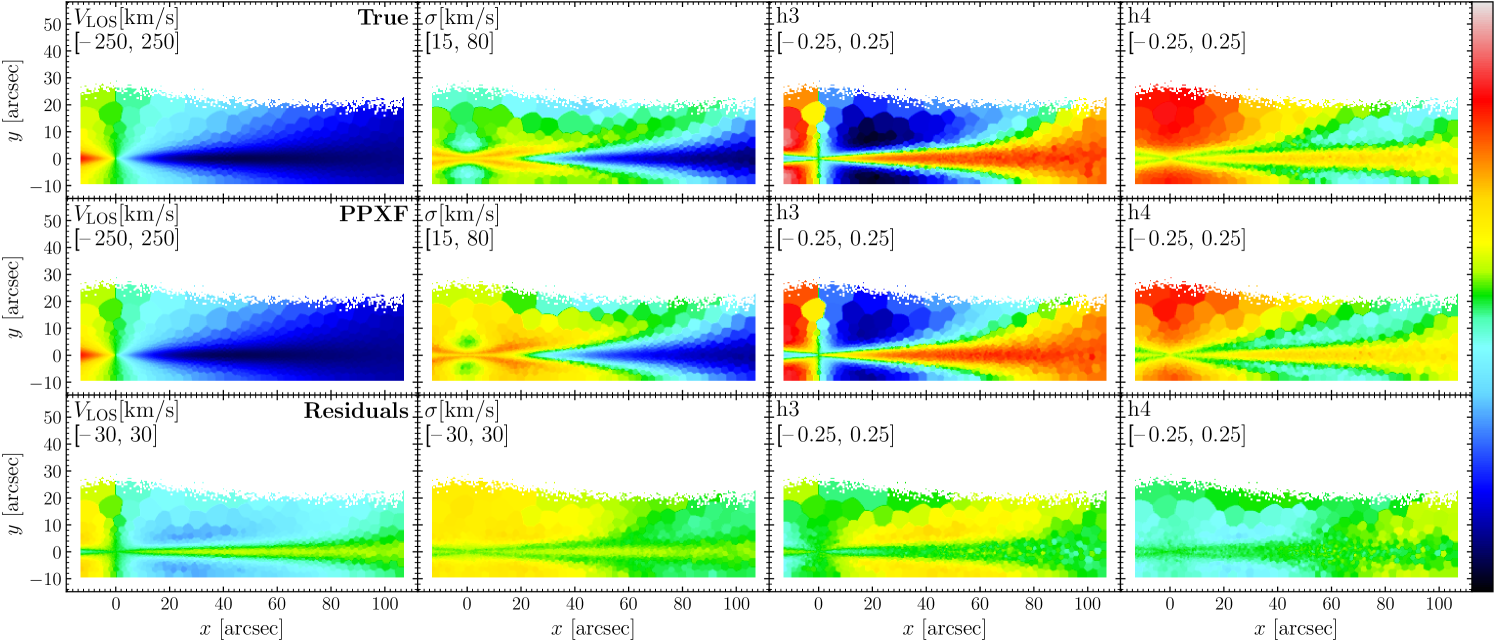
Figure 21: Same as Fig. 6 but for the mock cube generated and fitted by PEGASE-HR templates in PEGASE-HR spectral resolution ($\rm{FWHM}=0.55\Angstrom$).

To remove the effect of low spectral resolution, we tested the kinematics recovery again by using PEGASE-HR templates (Le Borgne et al., 2004) generated by Kroupa IMF and PADOVA 1994 isochrones, which has a higher spectral resolution ($\rm{FWHM}=0.55\Angstrom$) than MUSE ($\mathrm{FWHM}\sim 2.65\Angstrom$). The instrumental velocity scale of PEGASE-HR is $\sigma_{\rm inst}$$\sim 15$ km s^-1, which is smaller than the minimum $\sigma_{\rm{true}}$ of our Voronoi bins. We repeat all the procedures in Section 3.2 to generate new cubes using PEGASE-HR, and then apply them to the GIST pipeline to measure the kinematics. We keep the original PEGASE-HR spectral resolution throughout the whole process. The third row of Fig. 13 shows the kinematics recovery using PEGASE-HR (also see the kinematics map in Fig. 21). Compared to the first row, the residuals of each panel are slightly better or clearer when using higher spectral resolution templates. However, all these four moments from pPXF still have the same systematic offsets to the true values. Most improvements are for $h_{3}$ and $h_{4}$, with less bias to zero values because the higher spectral resolution helps identify skewness and kurtosis. We also show the results by turning off penalization in the fourth row (also see the kinematics map in Fig. 22), and find the $h_{3}$ and $h_{4}$ residuals are identical. Therefore, turning off penalization helps with low-spectral-resolution kinematics measurements, but does not affect higher-resolution spectra. The higher spectral resolution improves the kinematics recovery but does not fix the systematics offsets.

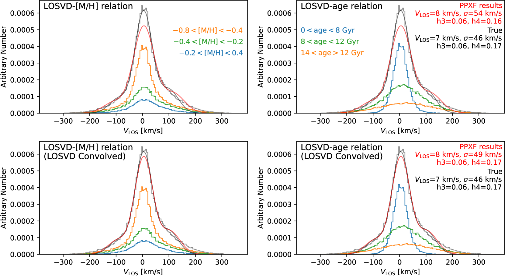
Figure 14: LOSVD of particles with different ages and $V_{\rm LOS}$ in one Voronoi bin. Particles are divided into three $[\mathrm{M/H}]$ and age groups, then their $V_{\rm LOS}$ histograms are plotted on the left and right panels in different colors, respectively. The grey histograms are the total $V_{\rm LOS}$ distributions of the three groups. The top rows are results using the original E-Galaxia catalog. The bottom rows are results from LOSVD-Convolved mock cubes. The red lines are pPXF results for mock cubes generated and fitted using PEGASE-HR templates in PEGASE-HR spectral resolution ($\rm{FWHM}=0.55\Angstrom$). The black lines are the true values calculated by fitting the Gauss-Hermite function with particles’ LOSVD in the black histogram. The kinematic parameters for these two lines are texted in the right top corner. This figure indicates LOSVD changes with age and $[\mathrm{M/H}]$, which disagrees with pPXF assuming LOSVD is a constant in a Voronoi bin. After using LOSVD-Convolved cubes, this relationship can be artificially eliminated, and pPXF can measure kinematic parameters accurately.

Fundamentally, during pPXF fitting process, SSP templates are loaded and convolved with a Gauss-Hermite function by FFT to match the observed spectrum (Cappellari, 2017), then it returns one series of LOSVD moments which are best fitted to the observed spectrum of each Voronoi bin. This means pPXF assumes all the templates having the same kinematics ($V_{\rm LOS}$, $\sigma$, $h_{3}$, $h_{4}$) in a line-of-sight, i.e., stellar populations with different $[\mathrm{M/H}]$ and ages are assumed to have the same LOSVD. But in real galaxies, due to the joint process of chemical enrichment and dynamical movements of stars, populations with different $[\mathrm{M/H}]$ and ages are different in LOSVDs. This effect is non-negligible for edge-on projected galaxies because metallicity and age gradients along the disk are the strongest. Therefore, $V_{\rm LOS}$ should change with $[\mathrm{M/H}]$ and age, which disagrees with the analysis used in most of the previous studies when employing pPXF. Because of the relation between $[\mathrm{\alpha/Fe}]$ and $[\mathrm{M/H}]$, stars with different $[\mathrm{\alpha/Fe}]$ should also have different $V_{\rm LOS}$.

To investigate it in our mock stellar catalog, we select one Voronoi bin and split the included particles into three groups using $[\mathrm{M/H}]$ and age, respectively. We reserve this investigation on $[\mathrm{\alpha/Fe}]$ for the future due to the limited number of $[\mathrm{\alpha/Fe}]$ templates. Then, we plot the LOSVDs of these groups of particles, weighted by each particle’s total flux, and show them in the first row of Fig. 14. In the top-left panel, particles with $-0.8<[\mathrm{M/H}]{}<-0.4$ dex have the sharpest distribution, while particles with $-0.2<[\mathrm{M/H}]{}<0.4$ dex show a nearly normal distribution. In the top-right panel, particles with $12<\rm{age}<14$ Gyr have the broadest distribution, while particles with $0<\rm{age}<8$ Gyr have the narrowest and most peaked distribution. The red line and black line represent pPXF fitted and the true LOSVD for this Voronoi bin, with kinematic parameters texted in the top right corner, respectively. Compared to the true LOSVD, the width of pPXF fitted curve in red is close to the youngest populations ($0<\rm{age}<8$ Gyr), which is reasonable because these populations dominate the light. However, the top right panel shows that pPXF tends to also care for the oldest populations by having a more skewed tail of their LOSVD at $V_{\rm LOS}$ around $150\sim 300$ km s^-1. Even though the youngest populations dominate the spectral light, the old populations have the most features along the whole fitted wavelength region. Therefore, the differences of the skewness in the region of $V_{\rm LOS}$ at $150\sim 300$ km s^-1 indicate the effect caused by different spectral features having different LOSVDs. This figure strongly suggests there are limitations on current techniques to obtain unbiased kinematics due to the dependence of $V_{\rm LOS}$ on age and $[\mathrm{M/H}]$.

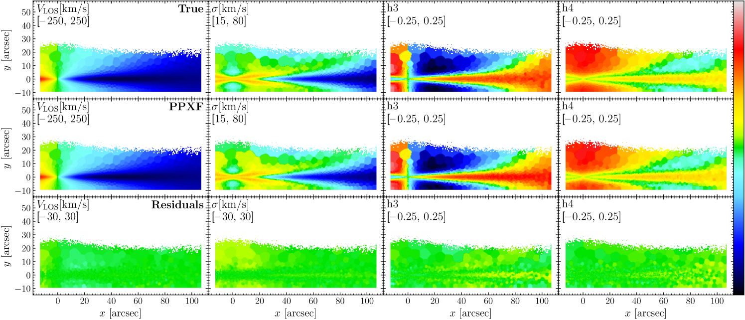
Figure 23: Same as Fig. 6 but for LOSVD-Convolved mock cubes generated and fitted by PEGASE-HR templates in PEGASE-HR spectral resolution ($\rm{FWHM}=0.55\Angstrom$).

We made a new experiment to verify this effect on pPXF results. Firstly, we re-generate mock MUSE cubes following the same procedures as above, but not using each particle’s $V_{\rm LOS}$ to shift the spectrum. In this way, we obtain non-kinematics mock data cubes. Next, for each Voronoi bin, we select all the particles included and obtain its $V_{\rm LOS}$ histogram, which is the true LOSVD as shown in grey in Fig. 14. Then, we directly use this histogram as the LOSVD kernel function and convolve it with all the spectra in this Voronoi bin to add kinematics. We do it for all the Voronoi bins and obtain new mock cubes, where spectral templates with different $[\mathrm{M/H}]$ and age have the same LOSVDs. Therefore, in this way, we eliminated the relation between $[\mathrm{M/H}]$ and ages as mentioned above. Finally, we employ pPXF to the new cubes (hereafter LOSVD-Convolved cubes) and measure the kinematics. The fifth row of Fig. 13 shows the kinematics recovery results. It is clear that all the Gauss-Hermite moments are well recovered with all the data points aligned to the zero line. The red and black lines in the bottom row of Fig. 14 also indicate the correction of pPXF measurements. We also plot the kinematics maps in the same way as Fig. 6 in Appendix (Fig. 23) to better demonstrate the consistency.

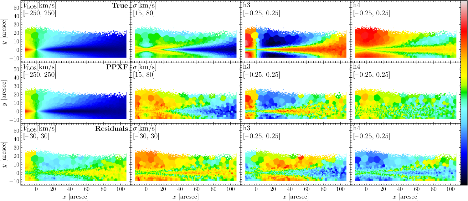
Figure 24: Same as Fig. 6 but for LOSVD-Convolved mock cubes generated and fitted using MILES templates in MUSE spectral resolution ($\rm{FWHM}=2.65\Angstrom$).

We also tested the kinematics recovery on LOSVD-Convolved cubes generated using MILES templates, as shown in the sixth row of Fig. 13 (see also Fig. 24). In this low spectral resolution, even though we make different populations have the same LOSVD for the spectra, there are still systematic offsets appearing in all the panels. We also demonstrate in the last row the results on LOSVD-Convolved cubes generated using PEGASE-HR templates, but in MUSE spectral resolution to remove the effects of different templates (see kinematics maps in Fig. 25). The appearance of offsets indicates the effect purely due to insufficient spectral resolution.

In conclusion, all these results strongly suggest that potentially both the low spectral resolution and variant LOSVD contribute to the systematic offsets we see in residual panels of Fig. 6. In the future, to remove the systematic offsets of stellar kinematics measured by pPXF, one needs to use an instrument with higher spectral resolution than MUSE. This means it is necessary to also increase the exposure time to achieve the same SNR. As we know $V_{\rm LOS}$ changes with $[\mathrm{M/H}]$ and age in the line-of-sight of real galaxy observations, it might be necessary to allow different templates to have different LOSVDs during the pPXF spectrum fitting to obtain more accurate results. However, since kinematic and stellar populations measurements via full spectrum fitting have already been a highly degenerate problem. Allowing variable LOSVDs will increase the degeneracy by a factor of the number of templates. In this case, the algorithm is easy to obtain incorrect results. One possible way would be simply assuming a quantitative relation between LOSVD and metallicity and age at different locations of the galaxy and that this relation can be expressed by an analytical equation. This is equivalent to adding a prior to the pPXF fitting process to improve the accuracy of kinematics measurement without adding degeneracy. Even though this way has many limitations, it will be still useful for the analysis of Milky-Way-like galaxies, and GalCraft can help provide this prior for galaxies in different projections.

Apart from the above analysis on pPXF inconsistencies with the true values, Fig. 14 also shows the disagreements between $V_{\rm LOS}$ histogram (grey line) and the parametrically best-fitted true LOSVD (black line). Even though it does not affect our conclusions above, we indicate the need for non-parametric techniques (e.g., BAYES-LOSVD Falcón-Barroso & Martig 2021) to measure kinematics rather than using Gauss-Hermite equation, especially for the $V_{\rm LOS}$ region of $150\sim 300$ km s^-1.

4.2 Inconsistency of Mass Fraction Distributions Recovery

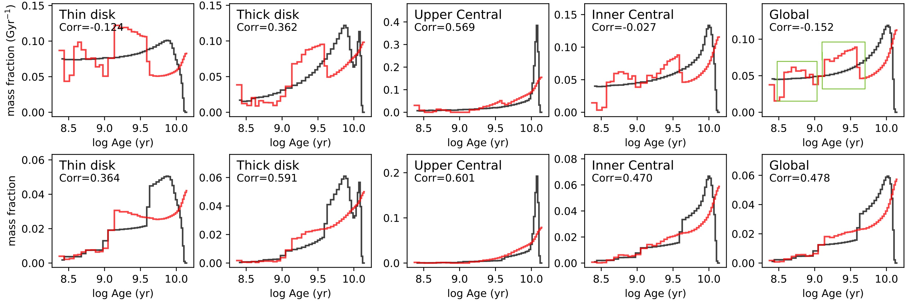
Figure 15: Age distribution recovery of different components of the galaxy from pPXF on the mock MUSE cube generated in Section 3.1. This figure is similar to Fig. 11 but the x-axis is in logarithmic scale. Black lines are the true values and red lines are the results from pPXF. The first row shows mass fraction $\text{Gyr}^{-1}$, which is the representation of star formation history, and the two green boxes in the “Global" panel are the two overdensity regions. The second row shows just the mass fraction, which is the direct output from pPXF. The correlation coefficients of the red and black lines are texted on the top right corner for each panel.

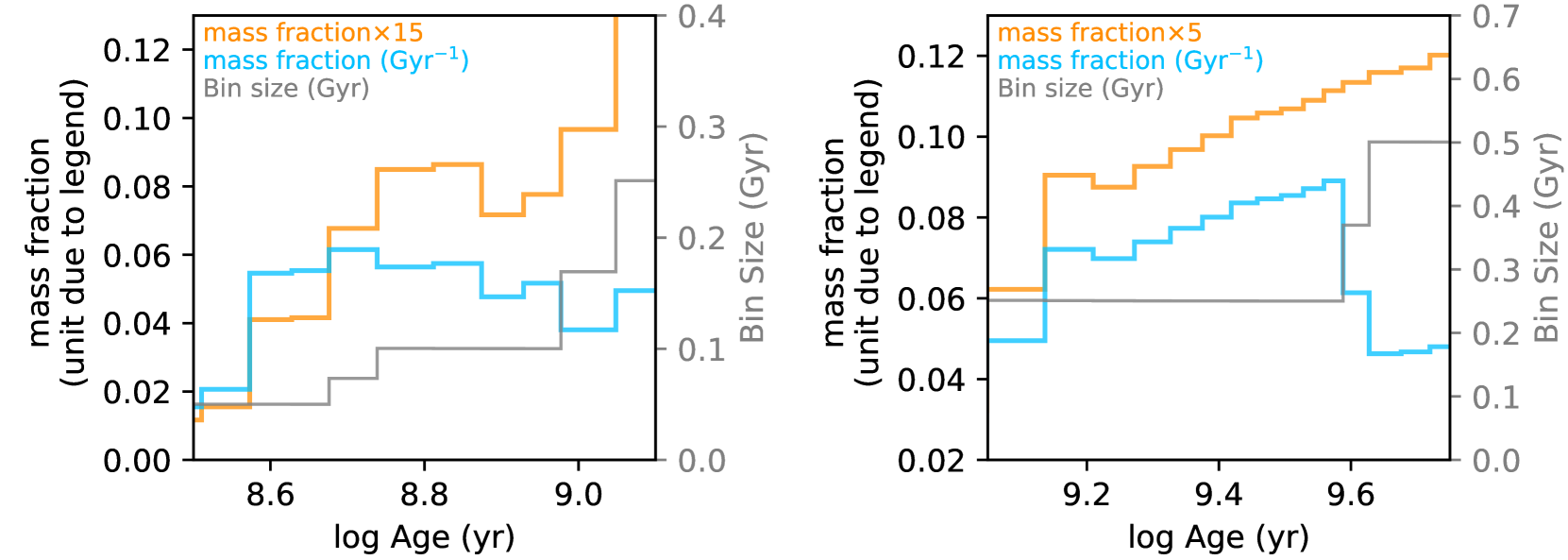
Figure 16: Zoom-in of the two overdensity regions pointed out in Fig. 15. The blue and orange lines are mass fraction ($\text{Gyr}^{-1}$) and mass fraction distributions, equivalent to the first and second row of Fig. 15, respectively. The mass fraction for each panel is multiplied by a factor for visualization. We also plot MILES templates’ age bin size as the grey line and the scale in the right y-axis.

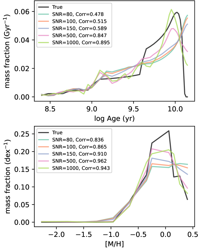
Figure 17: Global age (top panel) and $[\mathrm{M/H}]$ (bottom panel) distributions recovery at different SNRs, which are obtained by running pPXF on the mock MUSE cube generated in Section 3.1 with each target SNR of Voronoi bins, and then the mass fraction of all the bins are added together to represent the global mass distributions of the galaxy. Black lines are the true values. This figure indicates that increasing SNR can help obtain better mass distributions compared to the true values, especially the issue of metal-rich, old stellar population overestimation is alleviated.

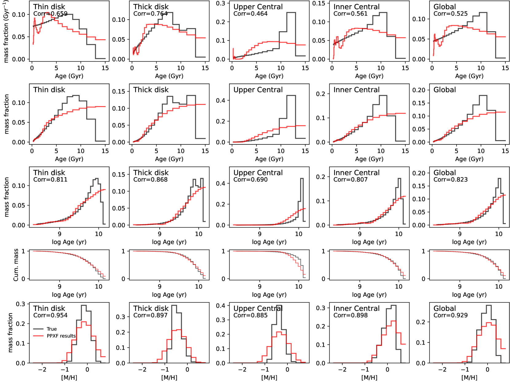
Figure 18: Age and $[\mathrm{M/H}]$ distributions of each component for the mock cubes generated using PEGASE-HR templates and degraded to MUSE resolution ($\rm{FWHM}=2.65\Angstrom$). The first row demonstrates mass fraction ($\text{Gyr}^{-1}$) changes with age (star formation history). The second row shows the mass fraction changes with age. The third row shows mass fraction changes with $\log\rm{age}$. The fourth row shows cumulative mass fraction distributions and the fifth row shows metallicity distributions.

In general spectral fitting, measuring mass fraction distributions of stellar populations is a highly degenerate problem, especially when one wants to obtain the star formation history of the Galaxy at different components. We follow the data analysis procedures in M21 to divide the template’s age and metallicity bin size. However, most of the previous studies did not consider the bin size. Nevertheless, the mass fractions increasing from young to old and metal-poor to metal-rich populations found in Fig. 11 is still seen in some components of the galaxies (e.g., Pinna et al. 2019a, b). In the mock and real data tests of Kacharov et al. (2018), the mass fraction distributions are also smoothed towards old and metal-rich regions (see their Fig. 5). The over-dense feature of young populations at around $2\sim 4$ Gyr in our Fig. 11 is also seen in some of the above-mentioned studies. In this section, we re-investigate all these tests more comprehensively using mock cubes of GalCraft and discuss the differences in the mass fraction distribution from pPXF, including whether or not to divide the templates’ age and metallicity bin size, and try to address potential reasons causing the inconsistency to the true values.

We first convert the age distribution x-axis of Fig. 11 from linear to log-scale, because MILES templates are almost evenly scaled in $\log\rm{age}$, then the width of each step is close to be equal. Next, we re-plot the age distribution recovery in Fig. 15 and calculate the correlation coefficients using the original age grids. The first row shows age distribution in mass fraction $\text{Gyr}^{-1}$, which is the representation of the star formation history of each component. The thin disk, inner central, and global panels clearly show two overdensity regions, which are pointed out by two green boxes. The thick disk and upper central panels also have peaky features in these boxes, but not significant. The second row shows just the mass fraction, which is the direct output from pPXF. Opposite the first row, all the panels in the second row show relatively smooth distributions. Therefore, given the differences between the first and second rows are whether or not dividing bin size, we speculate the two overdensity regions are artifacts due to the bin size arrangements to the template grids.

To verify our speculation, we plot in Fig. 16 a zoom-in of the two overdensity regions pointed out in the top right panel of Fig. 15. The blue and orange lines are mass fraction ($\text{Gyr}^{-1}$) and mass fraction distributions, equivalent to the first and second row of Fig. 15, respectively. The mass fraction for each panel is multiplied by a factor for better visualization. We also plot the age bin size of MILES templates as the grey line and the scale in the right y-axis. From these two panels, we find the peaky features of mass fraction ($\text{Gyr}^{-1}$) (blue line) appear when the age bin size experiences a decrease from old to young ages, and the mass fraction distribution (orange line) is still relatively smooth. Therefore, we can confirm the peaky features of star formation history from pPXF are due to the age bin size of templates. This also explains the better recovery of $[\mathrm{M/H}]$ distributions (bottom row of Fig. 11) which is due to the almost linearly spaced $[\mathrm{M/H}]$ grids.

Previous studies applied regularization (McDermid et al., 2015) in pPXF to obtain smooth mass fraction distributions. The regularization works as an extra term in the equation to be minimized during the optimization to damp high-frequency variations in the mass weights distribution along spectral templates grid (see details in Section 3.5 of Cappellari 2017) and leads to smooth mass weights distributions. However, the source code of pPXF indicates that this smoothness has an effect on mass weights rather than mass weights per bin size. This explains why mass fraction distributions are smooth in our results, and whether mass fraction ($\text{Gyr}^{-1}$) distributions are smooth depends on how the template grids are spaced. A further test by modifying pPXF and taking into account the bin size during regularization is needed to verify in the future. From now on, we only use the mass fraction without dividing the bin size to justify the recovery consistency, because this is expected to be achieved by pPXF.

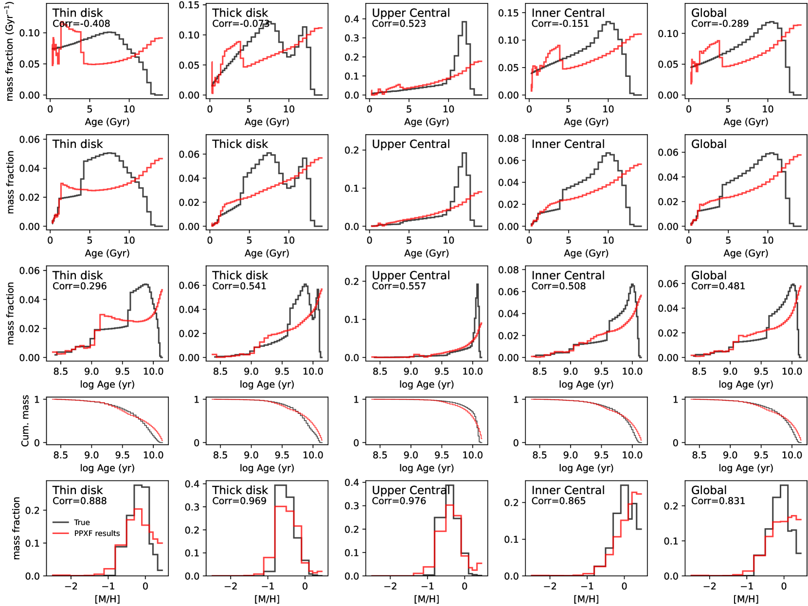
Figure 26: Same as Fig. 11 and Fig. 15 but for LOSVD-Convolved mock cubes generated using MILES templates in MUSE spectral resolution ($\rm{FWHM}=2.65\Angstrom$).

Although the current pPXF regularization algorithm does not consider the bin size of the template age grid and different regularization strategies (e.g., $R$ values, order of regularization) can affect the mass fraction recovery (will be discussed in Section 4.3), we still see the inconsistency between pPXF and true mass fraction distributions of the oldest populations in the bottom row of Fig. 15. The main reason is that spectral templates in the oldest and metal-rich regions are very similar and indistinguishable at the current SNR level. Therefore, the pPXF algorithm may get trapped into the local minimum when measuring mass fraction weights in these age-$[\mathrm{M/H}]$ regions. We also confirm in the Appendix (Fig. 26) that using LOSVD-Convolved cubes does not improve the results significantly.

One way to increase the quality of the mass fraction recovery in old and metal-rich population regions might be to increase the SNR of the spectrum. This can be achieved by requiring a higher target SNR during the process of Voronoi binning but with the cost of reducing the number of Voronoi bins, i.e., details in the parameter distributions. We show in Fig. 17 the age and $[\mathrm{M/H}]$ distributions at different SNRs (shown in different colors), compared to the true values shown in black lines. This figure is obtained by running the GIST pipeline on the mock MUSE cube generated in Section 3.1 with different target SNRs during Voronoi binning, and then the mass fraction distributions of all the Voronoi bins are added together to represent the global mass distributions of the galaxy, and finally integrated through age and $[\mathrm{M/H}]$ axes, respectively. To make it a fair comparison, we make sure that the spatial pixels used to generate Voronoi bins are the same. According to the correlation coefficients, this figure indicates that with the increase of Voronoi bin SNR, the global mass fraction distributions in both panels are more consistent with the true values. Specifically, the weights of metal-rich and old stellar populations are going lower with higher SNR. Therefore, Fig. 17 indicates that increasing SNR can improve SFH recovery. However, we note that in reality, an integrated spectrum with SNR larger than 1000 is impractical. In addition, even with SNR at 200 $\text{pix}^{-1}$ is pointless because in this case numerical issues, spectral library uncertainty, etc become the dominant factor.

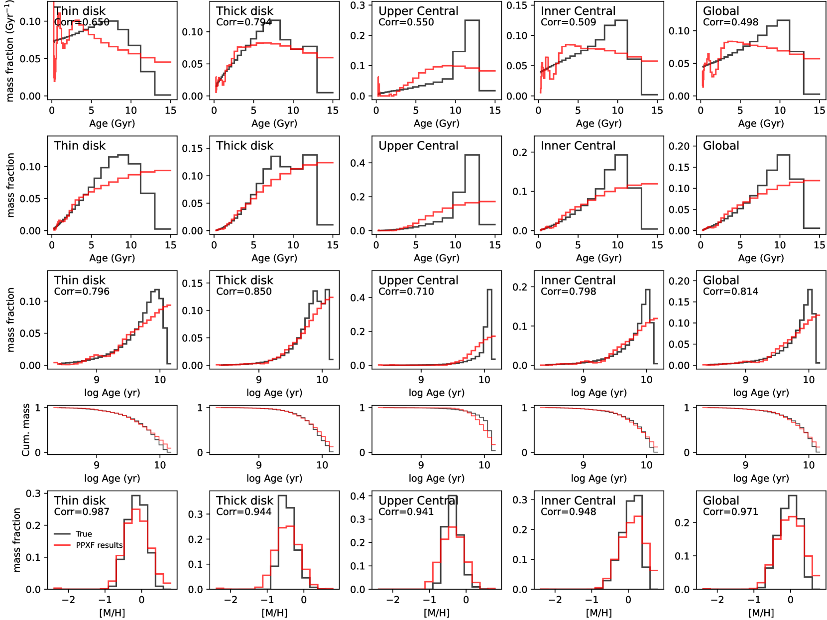
Figure 27: Same as Fig. 18 but for the mock cube generated using PEGASE-HR templates in PEGASE-HR spectral resolution ($\rm{FWHM}=0.55\Angstrom$).

To study the effect of different templates, we re-plot age and $[\mathrm{M/H}]$ distributions of mock cubes generated by PEGASE-HR templates in Fig 18. PEGASE-HR templates are evenly spaced in $\log\rm{age}$. During the pPXF fitting, we use the same templates and fitting strategies (fitting wavelength region, regularization, etc.) as those in Section 3.2 and also degrade to MUSE spectral resolution to remove the resolution differences (even though we find increasing spectral resolution does not improve the recovery significantly after comparing to Figure 27 of a PEGASE-HR spectral resolution version). The Voronoi bin allocation is the same as mock cubes generated by MILES templates. According to the correlation coefficients, mass fraction distribution using PEGASE-HR in Fig. 18 are more consistent than those using MILES in Fig. 11 and Fig. 15 for both age and $[\mathrm{M/H}]$. Moreover, the mass fraction - $\log\rm{age}$ panels (second row) have almost no blobs than the results using MILES (second row of Fig. 15), and the oldest populations have a more modest increase. Therefore, in our test, PEGASE-HR performs better during the mass fraction recovery and could provide more consistent mass fraction distributions than MILES. We think this is likely due to the templates’ perfectly even spacing in $\log\rm{age}$, which leads to smoother input and is preferred by pPXF during regularization. However, the PEGASE-HR templates used in our tests are generated using PADOVA 1994 (Bertelli et al., 1994) isochrones but MILES are generated using BASTI isochrones (Pietrinferni et al., 2004, 2006). Whether isochrones differences can affect mass fraction distribution recovery ability requires further investigations. Moreover, the current limitation of PEGASE-HR templates is they only have one bin in $[\mathrm{\alpha/Fe}]$, we emphasize here again the need for multiple $[\mathrm{\alpha/Fe}]$-grid templates.

In the future, non-parametrically, it is worthwhile to test the mass fraction recovery ability using a linearly spaced template grid or modifying pPXF to regularize the fitting in terms of mass weights per Gyr or dex. Parametrically, one can try to recover both chemical enrichment history and star formation history by taking into account chemical evolution theories, which will help remove counter-intuitive features in the mass fraction distributions. One approach is to use Bayesian spectral fitting codes, such as Prospector (Leja et al., 2017) or BAGPIPES (Carnall et al., 2018). Another example is the semi-analytic spectral fitting method from Zhou et al. (2022). This method applies full spectrum fitting with the predicted best-fit spectrum from chemical evolution models, which is similar to adding a prior on pPXF during the fitting. Fig. 6 of Zhou et al. (2022) showed that this method has better consistency on mass fraction recovery than pPXF, and the over-estimations in metal-rich, $2\sim 4$ and $12\sim 14$ Gyr regions are removed successfully. Therefore, it provides a way to measure chemical enrichment and SFH for future studies accurately. One important caveat is that their chemical evolution model is a close-box model, which does not apply to galaxies dominated by frequent passive merger events (e.g. NGC 7793 in Kacharov et al. 2018). In addition, this method does not take into account the relation of chemical abundances with velocity, which are important indicators for radial migration and kinematic heating.

4.3 Effect of Regularization

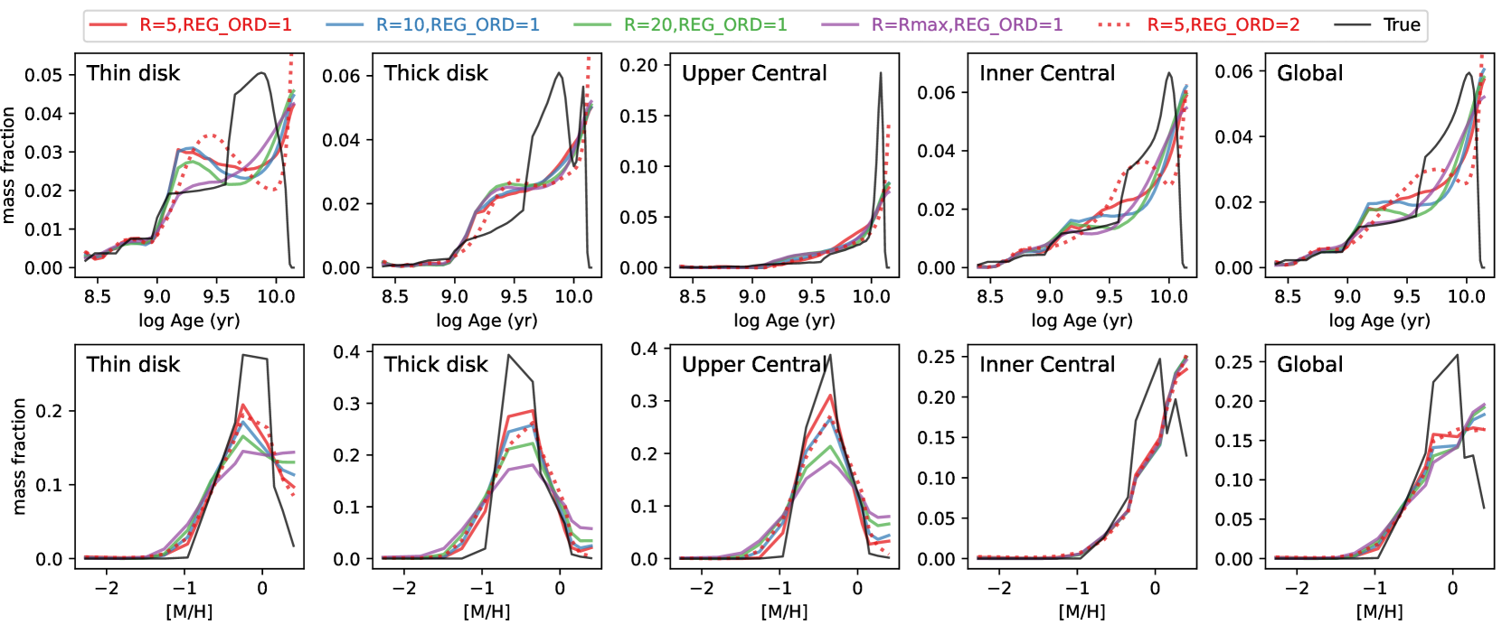
Figure 19: Age (top panel) and $[\mathrm{M/H}]$ (bottom panel) distributions recovery for different components of the galaxy by running pPXF on the mock MUSE cube generated in Section 3.1 with different regularization strategies (shown in different colors). Black lines are the true values. The last column shows global age and $[\mathrm{M/H}]$ distributions. This figure indicates that results using the first order of regularization are better than results using the second order of regularization; increasing $R$ can help obtain smoother results but the weights will go towards metal-rich regions for all the components.

In this section, we focus on the effects of different regularization strategies on mass fraction distributions. There are two parameters controlling the regularization in pPXF, which are regul and reg_ord, where regul or $R$ applies linear regularization to the weights during the pPXF fit and reg_ord controls the order of regularization. Kacharov et al. (2018) investigated mass fraction differences of mock data with different order of regularization (see their Fig. 5 and Fig. C2) and concluded that the choice of order of regularization does not affect the results over a significant level. Boecker et al. (2020) tested the mass fraction distributions recovery of the second- and third-order of regularization and compared them to the true values using stellar particles from an EAGLE simulated galaxy. They found results from third-order regularization are more consistent with the true values. Cappellari (2023) compared the mass fraction recovery consistency of non-regularized pPXF fit, an average of 100 pPXF fits to Montecarlo realizations, and single regularized pPXF fit (see their Fig. 1), and concluded that regularized results are comparable to that of the average of multiple realizations.

The selection of $R$ value was briefly discussed in Section 3.2. Here we re-investigate this question in detail by applying different regul and reg_ord strategies on our mock cubes generated in Section 3.1. The results are shown in Fig. 19, where we plot the age distributions on the top panels and $[\mathrm{M/H}]$ distributions on the bottom panels for different components of the galaxy. We also plot the global mass distributions in the last column. We apply five different strategies during the fitting: the first three cases use first-order regularization with $R=5$, $R=10$, $R=20$, and $R=R_{max}(30\sim 100)$, respectively; the last uses $R=5$ and second-order regularization. Black lines are the true values. When comparing results with the same order of regularization but different $R$, we find results with larger $R$ are smoother, and their weights at old populations are relatively smaller than results with smaller $R$. However, in the $[\mathrm{M/H}]$ distribution panels, weights are going more toward metal-rich populations and the distributions become less consistent with the true values for all the components. For results with the same $R$ but different orders of regularization, we see results with reg_ord $=1$ show better consistency with the true values than those with reg_ord $=2$. Specifically, results with reg_ord $=2$ have more mass fractions in the oldest populations.

In conclusion, Fig. 19 indicates that for this mock cube, results using the first order of regularization are better than results using the second order of regularization; increasing $R$ can help obtain smoother results but the weights will go towards metal-rich regions. Given we do not have the codes to perform third-order regularization, it is hard to say which order is the best. Intuitively, it seems higher-order regularization tends to have more mass fraction in the old populations. Therefore, we think the third-order regularization is preferred for EAGLE simulated galaxy test (Boecker et al., 2020) because the particles’ mass weights from the EAGLE simulations are naturally dominated by old and metal-rich populations, then the third-order regularization tends to fit better in this region. Our E-Galaxia mocked catalog has no particle in the metal-rich and oldest regions, so the first-order regularization is better. However, all the above discussions need further verification and we will test the third-order results in the future. For the real galaxy fitting results of Pinna et al. (2019a, b) and M21, they all used second-order regularization and showed an overdensity of mass weights in the oldest, metal-rich populations for different components of the galaxies, which makes it difficult to discuss differences in the formation epoch between these components, and it is not possible to tell if the overdensity is true or instead from pPXF artifacts.

4.4 Caveats when using GalCraft

In this section, we give some caveats when using the GalCraft code. Since this code is using the mock stellar catalog from E-Galaxia which embedded the GCE model of S21. The success of this model is that it can reproduce $[\mathrm{\alpha/Fe}]$-$[\mathrm{Fe/H}]$ bimodality which is quantitatively consistent with the APOGEE observations of the MW in Hayden et al. (2015). In reality, a more complex process is likely to exist as non-asymmetric perturbations such as spiral arms, bars, interlopers, etc. The current model does not have these features but can be added in the future; In addition, S21 suggests the $[\mathrm{\alpha/Fe}]$ bimodality is a natural result of radial migration and kinematic heating of stars, which is opposite to some clarifications by simulations which indicated that a merger is needed to contribute to the formation of bimodality (e.g., Clarke et al. 2019; Buck 2020), and this model lacks stars in the Galactic halo. Therefore, this code is not applicable for comparing the merger features or the halo distributions; This model also lacks descriptions of parameter distributions in the bulge, especially the nuclear disk in the MW center (e.g., Schultheis et al. 2021) and chemodynamics of the B/P bulge (e.g.. Wylie et al. 2021), which could be improved in the future.

5 Future Studies

In this study, we did not apply extinction on the mock data cube because this is the work purely on testing the kinematic and stellar populations recovery via full-spectrum fitting. In real edge-on galaxies, extinction can have an essential effect because it can obscure nearly 50% of the total light from stars in the thin disk, making SNR in this region lower. With the GalCraft code, we can test the kinematics and stellar population recovery of mock cubes with extinction. The extinction model in E-Galaxia is assumed as a double exponential distribution mainly in the thin disk, which can be integrated through the line-of-sight, and each particle will have a $E(B-V)$ value. Then, we can add the extinction effect to the spectrum by using a specific reddening curve (e.g., Cardelli et al. 1989; Calzetti et al. 2000), which is also the strategy that pPXF applies to estimate extinction. Ge et al. (2018) has already tested the effect of extinction on full-spectrum fitting results using one stellar population template, we can re-investigate it with a realistic E-Galaxia model and also study how different extinction models can affect the results. In addition, several non-asymmetric features should be added to the chemical evolution model like the spiral arms, bars, mergers, and halo particles to mimic a more realistic MW. It is also necessary to add gas emissions to GalCraft.

There are several improvements can be made to the choice of SSP models. The current version of GalCraft has embedded MILES and PEGASE-HR templates. In the future, we will add other empirical models such as BC03 (Bruzual & Charlot, 2003), X-Shooter (Verro et al., 2022), and theoretical models like STARBURST99 (Leitherer et al., 1999) and BPASS (Eldridge et al., 2017), which can satisfy different science goals since different models have different advantages. Some interesting tests can also be executed, e.g., using one SSP model to generate mock cubes and fit them with another model, which can help study the effect of SSP template uncertainties on full-spectrum fitting results.

In addition, even though we showed in Section 3.4 that the $[\mathrm{\alpha/Fe}]$-rich and $[\mathrm{\alpha/Fe}]$-poor populations can be well identified using two $[\mathrm{\alpha/Fe}]$ bins, it is still essential to add more bins to obtain detailed $[\mathrm{\alpha/Fe}]$ distributions. The Milky Way results in Hayden et al. (2015) have shown that stars in the thin and thick disk have $[\mathrm{\alpha/Fe}]$ values about $0.0$ and $0.2$ dex, respectively, and there are some stars with negative $[\mathrm{\alpha/Fe}]$, which is also shown in the E-Galaxia catalog. However, it is challenging to use current MILES $\alpha$-variable templates to identify these two $[\mathrm{\alpha/Fe}]$ sequences because most of the weights are in the bin of $[\mathrm{\alpha/Fe}]$ $=0$, and it is also difficult to assign a spectrum to particles with negative $[\mathrm{\alpha/Fe}]$. More $[\mathrm{\alpha/Fe}]$ bins (e.g., sMILES Knowles et al. 2023) will help on the study of $[\mathrm{\alpha/Fe}]$-$[\mathrm{M/H}]$ distributions for external galaxies at different components.

According to Section 4.1, given that spectral resolution is important in stellar kinematics measurements, it is also necessary to increase both the instruments’ and stellar population models’ spectral resolution. Current IFS observations such as MUSE perform well on kinematics measurements of the galaxies’ central region. However, to go deeper and obtain distributions of the outer regions, especially the outer thin disk, which normally has lower dispersion, one might need to use instruments and SSP templates with a higher spectral resolution to obtain more accurate kinematics maps.

Other than increasing spectral resolution. As discussed in Section 4.1, a prior can be added to the pPXF fitting process which assumes the relation between LOSVD and metallicity and age at different locations of the galaxy can be expressed by a function. Then it can allow templates to have different LOSVDs and the degeneracy is not increased. The other way is to add the evolution of stellar kinematics to the semi-analytic model like the one in Zhou et al. (2022) and make it derive the chemical evolution histories along with kinematic processes directly by fitting with the integrated spectra, where the fitting process is constrained by several model parameters and more physical. We will test the feasibility of these methods in the future.

As for mass fraction distributions, Section 4.2 demonstrated how the bin size can artificially create peaky features in the star formation history. In the future, it is worthwhile to test fitting results using linearly spaced template grids or modifying the pPXF algorithm on regularizing the fitting and considering the bin size in age and metallicity. Parametrical methods like Zhou et al. (2022) can also be used to test recovery abilities. Moreover, in this work, we inputted a smooth SFH for the tests. Whether the mass fraction distribution inconsistencies we found also apply to merger-dominated galaxies with multiple starburst phases can be investigated using GalCraft generated mock cubes of N-body/hydrodynamical simulations.

The aim of GalCraft code is to apply the knowledge we learned from the Milky Way to other Milky-Way-like galaxies by mocking the IFS observations as a bridge. Especially, we want to interpret physical processes such as radial migration, kinematic heating, and $[\mathrm{\alpha/Fe}]$-$[\mathrm{M/H}]$ distributions of other galaxies to answer the question of whether all the Milky Way analogs have similar processes to the MW, and if not, how much difference they can be. Therefore, when templates with more $[\mathrm{\alpha/Fe}]$ bins are available, we will perform a comparison of a mock Milky Way data cube from GalCraft with a real galaxy observation from the GECKOS survey (van de Sande et al., 2023), which will observe 35 edge-on Milky-Way-like galaxies, and see the feasibility of identifying these processes.

6 Summary and Conclusions

In this work, we present the GalCraft code which uses simple-stellar population models and the mock Milky Way catalog from E-Galaxia to generate a mock Milky Way data cube in the same data format as integral-field spectrograph (IFS) extra-galactic observations. We aim to eliminate the differences in analysis techniques between the Galactic and extra-galactic studies such as the use of individual stars vs. integrated stellar populations, the number density distributions of stars’ parameters vs. mass- or light-weighted distributions, the results with or without projection effect, etc. The mock data cube can be put into the GIST pipeline to perform data analysis in the same way as extra-galactic observations and the results can be compared directly to external galaxies to study the similarities and differences between the Milky Way and its analogs. Therefore, this code is a bridge to link the Galactic and extra-galactic studies to understand the formation and evolution of disk galaxies.

The GalCraft code is flexible, allowing users to choose their preferred SSP templates, galaxy distance and inclination, spatial/spectral resolution, and field-of-view of the instrument. GalCraft is also designed to mock current existing instrumental observations such as MUSE, SAMI, or MaNGA, as well as test the performance of future instrument designs. Moreover, it can also be applied to N-body/hydrodynamical simulations to generate mock observations.

For the rest of the paper, we applied pPXF on GalCraft generated mock cubes to test the ability of pPXF to recover the stellar kinematics and stellar population parameters. The mock MUSE data cubes have a distance of $26.5$ Mpc and inclination $86^{\circ}$, which is the same as NGC 5746 observations from M21.

After comparing the true values calculated from E-Galaxia particles’ properties with pPXF results, we found that there are systematic offsets between pPXF-recovered kinematic moments ($V_{\rm LOS}$, $\sigma$, $h_{3}$, $h_{4}$) and the true values. We confirm there are two reasons causing these offsets:

• The velocity dispersion $\sigma$ of most Voronoi bins are smaller than the instrument velocity dispersion $\sigma_{\rm inst}$ in MUSE spectral resolution ($\rm{FWHM}=2.65\Angstrom$).

• $V_{\rm LOS}$ changes with age and $[\mathrm{M/H}]$ for particles through the line-of-sight, but most previous studies assumed all stellar population templates have the same LOSVD during the pPXF fitting.

By using the higher spectral resolution templates PEGASE-HR ($\rm{FWHM}=0.55\Angstrom$) and applying the LOSVD-Convolved cubes which eliminate degeneracies of $V_{\rm LOS}$ with age and $[\mathrm{M/H}]$, we can obtain consistent kinematic results with the true values. Therefore, we indicate the need to allow different templates to have different LOSVDs or assume a quantitative relation between LOSVD and metallicity and age at different locations of the galaxy, where the equation coefficients can be measured during pPXF fitting. The latter method is equivalent to adding a prior to the pPXF fitting process to measure kinematics without adding degeneracy. We will perform tests on them and verify if kinematics recovery can be improved. In addition, our tests also indicate the need to use non-parametric methods such as BAYES-LOSVD (Falcón-Barroso & Martig, 2021) rather than Gauss-Hermite equation for more accurate measurements of $V_{\rm LOS}$ distributions.

In terms of stellar population parameters, we verified that pPXF can recover mass-weighted age, $[\mathrm{M/H}]$, and $[\mathrm{\alpha/Fe}]$ with good consistency. Both the $[\mathrm{\alpha/Fe}]$-rich and $[\mathrm{\alpha/Fe}]$-poor populations can be identified with reasonable regularization values during the fitting. Using line-strength indices can also identify these structures. We found mass fraction distributions of stellar populations from pPXF using MILES templates on MILES-generated mock cubes show deviations compared to the true values, where mass weights normalized by the bin size are overestimated in regions of $2\sim 4$ Gyr, $12\sim 14$ Gyr, the most metal-rich regions, and underestimated in regions of $5\sim 10$ Gyr. This could be due to many reasons including having low SNR that the flux error is larger than templates’ similarities in the region of old and metal-rich populations, the uneven spacing of age grids in MILES templates, current pPXF algorithm in regularization. These findings can be a reference for future extra-galactic data analysis of pPXF results on real galaxy observations. When repeating the test by employing pPXF and PEGASE-HR on PEGASE-HR-generated mock cubes, the mass fraction distributions are better with larger correlation coefficients between pPXF and true results, but differences still exist. In addition, we found using first-order regularization can obtain better mass fraction distributions than the second-order. Our tests and conclusions are helpful in identifying the limitations of studying some galaxy evolution processes using current methods and provide direction for potential improvements in the future.

Even though GalCraft provides a bridge to link the Galactic and extragalactic studies by transferring MW to mock IFS observations, there remains a need for future improvements to facilitate more accurate measurements of external galaxy properties such as $[\mathrm{\alpha/Fe}]$-bimodality and to enable detailed comparisons of the MW with MW-like galaxies. These improvements include more accurate SSP models with higher spectral resolution and more $[\mathrm{\alpha/Fe}]$ grids, more advanced spectral fitting algorithms, and instruments with deeper observations. Future tests using GalCraft are required including modifying pPXF codes to improve the recovery ability of kinematics and stellar population models, using templates with more $[\mathrm{\alpha/Fe}]$ grids, and adding extinction, to achieve measurements of known parameters such as radial migration and kinematic heating efficiencies of the MW in external galaxies.

Data Availability

GalCraft source code is publicly available via https://github.com/purmortal/galcraft. All the pPXF recovery test data and figures can be shared with reasonable requests.

Appendix A Modifications of the GIST pipeline

We provide a list of modifications on the GIST pipeline (Bittner et al., 2019) to improve the flexibility of this software: We add more templates such as the original and interpolated PEGASE-HR (Le Borgne et al., 2004) to the software and allow the option to oversample the spectra when degrading to lower observation spectral resolution, which is for the same reason as we do for the GalCraft code in Section 2.3; We also added the option to select SSP templates with a certain age and $[\mathrm{M/H}]$ range in some special cases. When measuring stellar kinematics and stellar population properties, we add the options to choose velscale_ratio, reg_ord, and use real spectra noise during the fitting and normalizing the integrated spectrum and noise by the median of the spectrum, which will be important to perform the iteration for estimating $R_{max}$; For regularization, we add an option to estimate $R_{max}$ following the procedures in McDermid et al. (2015) and save the stellar population results with $R=R_{max}$. We also allow further degrading to lower spectral resolution during the fitting when measuring SFH, which is mainly for the reduction procedures in M21 where they wanted to compare the mass-weighted stellar population parameters from pPXF with the SPP-equivalent parameters from line-strength indices in the same spectral resolution; We add the option to change the penalization value bias during pPXF fitting and measure mass weights uncertainties using bootstrapping following procedures in Kacharov et al. (2018).

Appendix B More Chemodynamic Parameters Recovery Results

Figure 20: Same as Fig. 6 but turning off the kinematics penalization during pPXF fitting.

Figure 22: Same as Fig. 21 but turning off the kinematics penalization during pPXF fitting.

Figure 25: Same as Fig. 6 but for LOSVD-Convolved mock cubes generated and fitted by PEGASE-HR templates in MUSE spectral resolution ($\rm{FWHM}=2.65\Angstrom$).

References

- Abdurro’uf et al. (2022) Abdurro’uf et al., 2022, ApJS, 259, 35
- Astropy Collaboration et al. (2013) Astropy Collaboration et al., 2013, A&A, 558, A33
- Astropy Collaboration et al. (2018) Astropy Collaboration et al., 2018, AJ, 156, 123
- Bacon et al. (2010) Bacon R., et al., 2010, in McLean I. S., Ramsay S. K., Takami H., eds, Society of Photo-Optical Instrumentation Engineers (SPIE) Conference Series Vol. 7735, Ground-based and Airborne Instrumentation for Astronomy III. p. 773508 (arXiv:2211.16795), doi:10.1117/12.856027
- Bertelli et al. (1994) Bertelli G., Bressan A., Chiosi C., Fagotto F., Nasi E., 1994, A&AS, 106, 275
- Bittner et al. (2019) Bittner A., et al., 2019, A&A, 628, A117
- Bland-Hawthorn & Gerhard (2016) Bland-Hawthorn J., Gerhard O., 2016, ARA&A, 54, 529
- Boardman et al. (2020) Boardman N., et al., 2020, MNRAS, 491, 3672
- Boecker et al. (2020) Boecker A., Leaman R., van de Ven G., Norris M. A., Mackereth J. T., Crain R. A., 2020, MNRAS, 491, 823
- Bruzual & Charlot (2003) Bruzual G., Charlot S., 2003, MNRAS, 344, 1000
- Buck (2020) Buck T., 2020, MNRAS, 491, 5435
- Buder et al. (2021) Buder S., et al., 2021, MNRAS, 506, 150
- Bundy et al. (2015) Bundy K., et al., 2015, ApJ, 798, 7
- Calzetti et al. (2000) Calzetti D., Armus L., Bohlin R. C., Kinney A. L., Koornneef J., Storchi-Bergmann T., 2000, ApJ, 533, 682
- Cappellari (2017) Cappellari M., 2017, MNRAS, 466, 798
- Cappellari (2023) Cappellari M., 2023, MNRAS, 526, 3273
- Cappellari & Copin (2003) Cappellari M., Copin Y., 2003, MNRAS, 342, 345
- Cappellari & Emsellem (2004) Cappellari M., Emsellem E., 2004, PASP, 116, 138
- Cardelli et al. (1989) Cardelli J. A., Clayton G. C., Mathis J. S., 1989, ApJ, 345, 245
- Carnall (2017) Carnall A. C., 2017, arXiv e-prints, p. arXiv:1705.05165
- Carnall et al. (2018) Carnall A. C., McLure R. J., Dunlop J. S., Davé R., 2018, MNRAS, 480, 4379
- Chabrier (2003) Chabrier G., 2003, PASP, 115, 763
- Chiappini et al. (1997) Chiappini C., Matteucci F., Gratton R., 1997, ApJ, 477, 765
- Clarke et al. (2019) Clarke A. J., et al., 2019, MNRAS, 484, 3476
- Comerón et al. (2018) Comerón S., Salo H., Knapen J. H., 2018, A&A, 610, A5
- Conroy (2013) Conroy C., 2013, ARA&A, 51, 393
- Croom et al. (2012) Croom S. M., et al., 2012, MNRAS, 421, 872
- Eldridge et al. (2017) Eldridge J. J., Stanway E. R., Xiao L., McClelland L. A. S., Taylor G., Ng M., Greis S. M. L., Bray J. C., 2017, Publ. Astron. Soc. Australia, 34, e058
- Elmegreen & Shadmehri (2003) Elmegreen B. G., Shadmehri M., 2003, MNRAS, 338, 817
- Falcón-Barroso & Martig (2021) Falcón-Barroso J., Martig M., 2021, A&A, 646, A31
- Foreman-Mackey et al. (2013) Foreman-Mackey D., Hogg D. W., Lang D., Goodman J., 2013, PASP, 125, 306
- Fraser-McKelvie et al. (2019) Fraser-McKelvie A., Merrifield M., Aragón-Salamanca A., 2019, MNRAS, 489, 5030
- Freeman & Bland-Hawthorn (2002) Freeman K., Bland-Hawthorn J., 2002, ARA&A, 40, 487
- Gaia Collaboration et al. (2023) Gaia Collaboration et al., 2023, A&A, 674, A1
- Ge et al. (2018) Ge J., Yan R., Cappellari M., Mao S., Li H., Lu Y., 2018, MNRAS, 478, 2633
- Girardi et al. (2000) Girardi L., Bressan A., Bertelli G., Chiosi C., 2000, A&AS, 141, 371
- Girardi et al. (2005) Girardi L., Groenewegen M. A. T., Hatziminaoglou E., da Costa L., 2005, A&A, 436, 895
- Guérou et al. (2016) Guérou A., Emsellem E., Krajnović D., McDermid R. M., Contini T., Weilbacher P. M., 2016, A&A, 591, A143
- Harris et al. (2020) Harris C. R., et al., 2020, Nature, 585, 357
- Hayden et al. (2015) Hayden M. R., et al., 2015, ApJ, 808, 132
- Haywood et al. (2018) Haywood M., Di Matteo P., Lehnert M., Snaith O., Fragkoudi F., Khoperskov S., 2018, A&A, 618, A78
- Haywood et al. (2019) Haywood M., Snaith O., Lehnert M. D., Di Matteo P., Khoperskov S., 2019, A&A, 625, A105
- Hopkins et al. (2018) Hopkins P. F., et al., 2018, MNRAS, 480, 800
- Hunter (2007) Hunter J. D., 2007, Computing in Science and Engineering, 9, 90
- Kacharov et al. (2018) Kacharov N., Neumayer N., Seth A. C., Cappellari M., McDermid R., Walcher C. J., Böker T., 2018, MNRAS, 480, 1973
- Knowles et al. (2023) Knowles A. T., Sansom A. E., Vazdekis A., Allende Prieto C., 2023, MNRAS, 523, 3450
- Koleva et al. (2009) Koleva M., Prugniel P., Bouchard A., Wu Y., 2009, A&A, 501, 1269
- Krajnović et al. (2008) Krajnović D., et al., 2008, MNRAS, 390, 93
- Kroupa (2001) Kroupa P., 2001, MNRAS, 322, 231
- Kubryk et al. (2015) Kubryk M., Prantzos N., Athanassoula E., 2015, A&A, 580, A126
- Kuntschner et al. (2006) Kuntschner H., et al., 2006, MNRAS, 369, 497
- Le Borgne et al. (2004) Le Borgne D., Rocca-Volmerange B., Prugniel P., Lançon A., Fioc M., Soubiran C., 2004, A&A, 425, 881
- Leitherer et al. (1999) Leitherer C., et al., 1999, ApJS, 123, 3
- Leja et al. (2017) Leja J., Johnson B. D., Conroy C., van Dokkum P. G., Byler N., 2017, ApJ, 837, 170
- Lian et al. (2020) Lian J., et al., 2020, MNRAS, 497, 2371
- Licquia & Newman (2016) Licquia T. C., Newman J. A., 2016, ApJ, 831, 71
- Licquia et al. (2015) Licquia T. C., Newman J. A., Brinchmann J., 2015, ApJ, 809, 96
- Licquia et al. (2016) Licquia T. C., Newman J. A., Bershady M. A., 2016, ApJ, 833, 220
- Mackereth et al. (2018) Mackereth J. T., Crain R. A., Schiavon R. P., Schaye J., Theuns T., Schaller M., 2018, MNRAS, 477, 5072
- Majewski et al. (2017) Majewski S. R., et al., 2017, AJ, 154, 94
- Martig et al. (2021) Martig M., et al., 2021, MNRAS, 508, 2458
- Martín-Navarro et al. (2018) Martín-Navarro I., Vazdekis A., Falcón-Barroso J., La Barbera F., Yıldırım A., van de Ven G., 2018, MNRAS, 475, 3700
- Martínez-Lombilla & Knapen (2019) Martínez-Lombilla C., Knapen J. H., 2019, A&A, 629, A12
- McDermid et al. (2015) McDermid R. M., et al., 2015, MNRAS, 448, 3484
- Minchev et al. (2013) Minchev I., Chiappini C., Martig M., 2013, A&A, 558, A9
- Mutch et al. (2011) Mutch S. J., Croton D. J., Poole G. B., 2011, ApJ, 736, 84
- Nidever et al. (2014) Nidever D. L., et al., 2014, ApJ, 796, 38
- Pietrinferni et al. (2004) Pietrinferni A., Cassisi S., Salaris M., Castelli F., 2004, ApJ, 612, 168
- Pietrinferni et al. (2006) Pietrinferni A., Cassisi S., Salaris M., Castelli F., 2006, ApJ, 642, 797
- Pinna et al. (2019a) Pinna F., et al., 2019a, A&A, 623, A19
- Pinna et al. (2019b) Pinna F., et al., 2019b, A&A, 625, A95
- Pinna et al. (2021) Pinna F., et al., 2021, ApJ, 921, 8
- Prugniel & Soubiran (2001) Prugniel P., Soubiran C., 2001, A&A, 369, 1048
- Prugniel et al. (2007) Prugniel P., Soubiran C., Koleva M., Le Borgne D., 2007, arXiv e-prints, pp astro–ph/0703658
- Salpeter (1955) Salpeter E. E., 1955, ApJ, 121, 161
- Sánchez et al. (2012) Sánchez S. F., et al., 2012, A&A, 538, A8
- Sanders & Binney (2015) Sanders J. L., Binney J., 2015, MNRAS, 449, 3479
- Schaye et al. (2015) Schaye J., et al., 2015, MNRAS, 446, 521
- Schiavon (2007) Schiavon R. P., 2007, ApJS, 171, 146
- Schönrich & Binney (2009) Schönrich R., Binney J., 2009, MNRAS, 396, 203
- Schultheis et al. (2021) Schultheis M., et al., 2021, A&A, 650, A191
- Scott et al. (2021) Scott N., van de Sande J., Sharma S., Bland-Hawthorn J., Freeman K., Gerhard O., Hayden M. R., McDermid R., 2021, ApJ, 913, L11
- Serra & Trager (2007) Serra P., Trager S. C., 2007, MNRAS, 374, 769
- Sharma et al. (2011) Sharma S., Bland-Hawthorn J., Johnston K. V., Binney J., 2011, ApJ, 730, 3
- Sharma et al. (2021a) Sharma S., et al., 2021a, MNRAS, 506, 1761
- Sharma et al. (2021b) Sharma S., Hayden M. R., Bland-Hawthorn J., 2021b, MNRAS, 507, 5882
- Shu (1969) Shu F. H., 1969, ApJ, 158, 505
- Spitoni et al. (2019) Spitoni E., Silva Aguirre V., Matteucci F., Calura F., Grisoni V., 2019, A&A, 623, A60
- Thomas et al. (2011) Thomas D., Maraston C., Johansson J., 2011, MNRAS, 412, 2183
- Trager & Somerville (2009) Trager S. C., Somerville R. S., 2009, MNRAS, 395, 608
- Vazdekis (1999) Vazdekis A., 1999, ApJ, 513, 224
- Vazdekis et al. (1996) Vazdekis A., Casuso E., Peletier R. F., Beckman J. E., 1996, ApJS, 106, 307
- Vazdekis et al. (2010) Vazdekis A., Sánchez-Blázquez P., Falcón-Barroso J., Cenarro A. J., Beasley M. A., Cardiel N., Gorgas J., Peletier R. F., 2010, MNRAS, 404, 1639
- Vazdekis et al. (2015) Vazdekis A., et al., 2015, MNRAS, 449, 1177
- Verro et al. (2022) Verro K., et al., 2022, A&A, 661, A50
- Virtanen et al. (2020) Virtanen P., et al., 2020, Nature Methods, 17, 261
- Worthey (1994) Worthey G., 1994, ApJS, 95, 107
- Wylie et al. (2021) Wylie S. M., Gerhard O. E., Ness M. K., Clarke J. P., Freeman K. C., Bland-Hawthorn J., 2021, A&A, 653, A143
- Xiang & Rix (2022) Xiang M., Rix H.-W., 2022, Nature, 603, 599
- Yniguez et al. (2014) Yniguez B., Garrison-Kimmel S., Boylan-Kolchin M., Bullock J. S., 2014, MNRAS, 439, 73
- Yoachim & Dalcanton (2006) Yoachim P., Dalcanton J. J., 2006, AJ, 131, 226
- Zhao et al. (2012) Zhao G., Zhao Y.-H., Chu Y.-Q., Jing Y.-P., Deng L.-C., 2012, Research in Astronomy and Astrophysics, 12, 723
- Zhou et al. (2022) Zhou S., Merrifield M., Aragón-Salamanca A., 2022, MNRAS, 513, 5446
- Zhou et al. (2023) Zhou S., Aragón-Salamanca A., Merrifield M., Andrews B. H., Drory N., Lane R. R., 2023, MNRAS, 521, 5810
- van de Sande et al. (2017) van de Sande J., et al., 2017, ApJ, 835, 104
- van de Sande et al. (2023) van de Sande J., Fraser-McKelvie A., Fisher D. B., Martig M., Hayden M. R., the GECKOS Survey collaboration 2023, arXiv e-prints, p. arXiv:2306.00059