Collisional shift and broadening of Rydberg states in nitric oxide at room temperature

Abstract

We report on the collisional shift and line broadening of Rydberg states in nitric oxide (NO) with increasing density of a background gas at room temperature. As a background gas we either use NO itself or nitrogen (N₂). The precision spectroscopy is achieved by a sub-Doppler three-photon excitation scheme with a subsequent readout of the Rydberg states realized by the amplification of a current generated by free charges due to collisions. The shift shows a dependence on the rotational quantum state of the ionic core and no dependence on the principle quantum number of the orbiting Rydberg electron. The experiment was performed in the context of developing a trace–gas sensor for breath gas analysis in a medical application.

I Introduction

By the end of the 1980s it was known, that NO plays an important role in the mammalian system [1, 2, 3]. This lead to the Nobel prize in Physiology or Medicine being awarded to Murad, Furchgott and Ignarro in 1998 for their discovery [4], which ultimately paved the way to a broad field of research [5], involving results on different forms of cancer [6, 7, 8, 9] and the role of NO in immunological responses such as inflammation [10]. That NO is also part of the exhaled breath, was shown in 1991 by Gustafsson et al. [11], and subsequent research revealed a change in the NO concentration when diseases like asthma, atopy and others are present [12]. The NO concentration in the exhaled breath is in the low ppb–regime, and a guideline [12] suggests that a sensor for breath–gas analysis must be calibrated with samples in the range of $10\text{\,}\mathrm{ppb}$ to $100\text{\,}\mathrm{ppb}$. Such a requirement is challenging when considering, that low gas volumes are preferred. For example, [12] states, that a patient has to exhale for $10\text{\,}\mathrm{s}$ at a constant flow to gain about $300\text{\,}\mathrm{ml}$ of air volume for sensors readily available. In the context of medical research such volumes are expected to be way lower.

We demonstrated a proof–of–concept experiment for a sensor based on the Rydberg excitation of NO in [13], capable of detecting NO concentrations less than $10\text{\,}\mathrm{ppm}$ limited by preparation, and yet operable at ambient pressure. The extrapolated sensitivity already reached the $10\text{\,}\mathrm{ppb}$ range. Here, only pulsed laser systems were used. In the experiment presented in this work only continuous–wave (cw) laser systems are used for the excitation of NO. This ensures selective detection due to the linewidth of cw systems. Our goal in this work is to learn about consequences for the sensor application. As such we investigate collisional shifts and broadening of the Rydberg line with increasing density of the background gas. This allows us to compare our results with previous results gained in the scope of the investigation of elastic scattering as theoretically introduced by Fermi [14] and investigated within the scope of the scattering length [15, 16]. In a wider context, the consequential improvement in sensitivity may enable us to detect Rydberg bimolecules of NO in the future, which have been predicted theoretically [17].

II Methods

Setup

A sketch of the main components of the experimental setup is shown in figure 1.

Figure 1: Sketch of the setup and measurement principle used throughout this work. Gas mixtures of a certain concentration of NO diluted in N₂, or pure NO enter the measurement cell on the left. Excitation of NO to a Rydberg state is achieved by a cw three–laser excitation scheme shown on the upper left. Subsequent collisions ionize these molecules. Charges are collected via electrodes, and the current is amplified and converted to a voltage by employing a transimpedance amplifier (TIA). A lock-in amplifier referenced on the modulated second transition improves the signal–to–noise ratio (SNR). The cell’s cuboid has a width of $35\text{\,}\mathrm{mm}$, a depth of $13.5\text{\,}\mathrm{mm}$, and a height of $8.4\text{\,}\mathrm{mm}$. Pictures are shown in figure 2.

All measurements are performed at room temperature, $T\approx$293\text{\,}\mathrm{K}$$. The detection of Rydberg states in NO is realized by the electronic detection of free charges. As such the central part of our setup is a custom designed glass cell with built–in readout electronics.

The cell’s glass frame has a copper plate glued to the bottom, whereas the top holds a printed-circuit board (PCB) with an electrode pointing towards the cell’s interior and amplification electronics on the other side. Pictures are shown in figure 2. Gas may flow through the cell as flange connectors are to the left and right of the frame. Applying a (possibly small) potential to bottom and top electrodes collects free charges within the cell, and the needed amplification and conversion to a voltage of the current is achieved by the use of a transimpedance amplifier (TIA) with an overall feedback resistance of $1\text{\,}\mathrm{G\SIUnitSymbolOhm}$. The electrodes have an area of about $472\text{\,}{\mathrm{mm}}^{2}$.

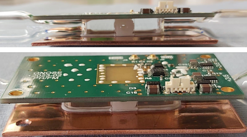
Figure 2: Pictures of the readout cell. In the center of the upper photo we can see the quartz windows, which are glued to the glass frame, such that the UV–light may pass through. On the left and right are the attachments to the MFCs and pumps. The lower photo shows the PCB with readout electronics on top, as well as a copper plate on the bottom, which realizes the counterelectrode.

While a constant and homogeneous field between the electrodes is desirable, a large area of the upper electrode connected to the TIA’s input results in a large antenna collecting noise from surrounding sources. Thus, a trade-off has to be made between the two. Our solution is to divide the electrode up into sections, which are all hold at the same potential. This is indicated in figure 1 on the top electrode. In our setup, the outermost part is a solder-resist free ground plane, then an actively driven guard ring follows, and the innermost area centered above the excitation volume is connected to the TIA. This area has dimensions $$13.5\text{\,}\mathrm{mm}$\times$10\text{\,}\mathrm{mm}$$, where the longer side is parallel to the laser beams.

Pressure stability is achieved by using mass-flow controllers (MFC) between the gas bottles and the experimental cell. Two MFCs are used for the experiment, one allows to regulate the flow of NO in the range of $0.1\text{\,}\mathrm{sccm}$ to $5\text{\,}\mathrm{sccm}$, and the other regulates the (optional) flow of N₂ in a range of $1.6\text{\,}\mathrm{sccm}$ to $100\text{\,}\mathrm{sccm}$. If only pure NO is used, the other MFC is closed off by valves. The pressure is constantly monitored at both ends of the cell by pressure gauges.

The NO molecules are excited to a Rydberg state by a three-photon excitation scheme solely by continuous-wave (cw) laser systems shown on the top left in figure 1. We only operate on transitions, where the vibrational quantum $v$ is $v=0$. While the ultraviolet (UV) beam enters the cell on the rear, the two other lasers are counter-propagating entering from the front. Subsequent collisions of the excited NO molecules with other particles yield free charges, which are electronically detected. The UV system, a frequency-quadrupled titanium-sapphire laser (Ti:sa), was already introduced in our previous work [18], and is used to drive the first transition, $\text{A}\,{}^{2}\Sigma^{+}\leftarrow\text{X}\,{}^{2}\Pi_{3/2}$. The $1/e^{2}$ beam waist $w$ is about $940\text{\,}\mathrm{\SIUnitSymbolMicro m}$, and the mean intensity $I=P/\pi w^{2}$ is on average $1.8\text{\,}\mathrm{mW}\text{\,}{\mathrm{mm}}^{-2}$. The cw light for the second transition $\text{H}\,{}^{2}\Sigma^{+}\leftarrow\text{A}\,{}^{2}\Sigma^{+}$ is generated by a $1080\text{\,}\mathrm{nm}$ diode laser, which is fiber–amplified and finally frequency-doubled via a single-pass periodically-poled lithium niobate crystal (PPLN). The beam has a waist of about $640\text{\,}\mathrm{\SIUnitSymbolMicro m}$ and an intensity of on average $480\text{\,}\mathrm{mW}\text{\,}{\mathrm{mm}}^{-2}$. The light for the Rydberg transition $n(N^{+})\leftarrow\text{H}\,{}^{2}\Sigma^{+}$ is another Ti:sa with a beam waist of $1220\text{\,}\mathrm{\SIUnitSymbolMicro m}$ used at an intensity ranging from $47\text{\,}\mathrm{mW}\text{\,}{\mathrm{mm}}^{-2}$ to $66\text{\,}\mathrm{mW}\text{\,}{\mathrm{mm}}^{-2}$. Note that all beam waist measurements are the average value of values gathered $10\text{\,}\mathrm{cm}$ in front and after the cell. The intensities are measured directly before entering the cell.

Our setup consists of a separate stabilization setup based on a reference laser at $780\text{\,}\mathrm{nm}$ locked to an ultra-low expansion cavity and then used to stabilize the length of transfer cavities. This allows to lock the fundamental beams of our excitation lasers to their respective transfer cavities. The Rydberg laser is not locked but scanned during the experiment, and its locked transfer cavity serves as a relative frequency reference. The whole stabilization setup is based on several Red Pitaya STEMlab 125-14A and a self-written lock software built on top of PyRPL [19]. A thorough walkthrough is given in [20]. Additionally, all fundamental beams are sent to a wavemeter (HighFinesse WS-6) for monitoring.

An improvement in the signal–to–noise ratio (SNR) is gained by using a lock-in amplifier referenced by the modulation frequency of the second transition. Modulation of the second transition itself is achieved by an acousto-optic modulator (AOM), which is driven by the amplified signal of a Red Pitaya STEMlab 125-14A.

Experimental procedure

After evacuating the cell by using a backing pump and a turbo pump to about $1\text{\cdot}{10}^{-5}\text{\,}\mathrm{mbar}$ a constant flow of gas and thus a constant pressure is ensured by the MFCs. Two measurement types are performed, either using pure NO or with mixtures of NO and N₂. As soon as a stable pressure is achieved, the lasers for $\text{A}\,{}^{2}\Sigma^{+}\leftarrow\text{X}\,{}^{2}\Pi_{3/2}$ and $\text{H}\,{}^{2}\Sigma^{+}\leftarrow\text{A}\,{}^{2}\Sigma^{+}$ are locked to their respective branches. For the UV transition this is the $\text{P}_{12}(6.5)$ branch at roughly $226.982\text{\,}\mathrm{nm}$, and for the intermediate transition the $R_{11}(5.5)$ at about $540.494\text{\,}\mathrm{nm}$ is used. The wavelengths given are the wavemeter’s readout, which has an inaccuracy of $600\text{\,}\mathrm{MHz}$. The initial value of the UV transition was at first simulated with PGOPHER [21] by using constants from [22]. The initial wavelength of the branch $R_{11}(5.5)$ of the second transition was taken from [23].

Finding the locked transitions is achieved by scanning and electronically reading out the signal as well. Here, we use higher pressures, about $1\text{\,}\mathrm{mbar}$, and higher fields, about $10\text{\,}\mathrm{V}\text{\,}{\mathrm{cm}}^{-1}$. As soon as both transitions are locked the pressure is set a little lower to about $60\text{\,}\mathrm{\SIUnitSymbolMicro bar}$ to ease finding the Rydberg signal, since this avoids significant broadening. On top, we set the applied field low to about $-0.8\text{\,}\mathrm{V}\text{\,}{\mathrm{cm}}^{-1}$, thus no significant splitting of the state due to the Stark effect occurs. The Rydberg signal is obtained by scanning the Ti:sa operating on $n(N^{+})\leftarrow\text{H}\,{}^{2}\Sigma^{+}$. Throughout the whole measurement we scan the Rydberg laser and trigger the scope on its ramp. Finally, the pressure is set via the MFC to the desired start pressure. Due to positions of the gauges, the pressure inside the cell cannot be known exactly. However, a bypass of the cell allows setting inbound and outbound pressure close to each other. Thus, we assume the pressure inside the cell to be the mean of both measured values.

For our measurements we are able to choose the principal quantum number $n$ as well as the rotational quantum number of the ionic core $N^{+}$ of Rydberg states in NO. A state is denoted by $n(N^{+})$, and we omit specifying the ionic part $\text{X}^{+}\,{}^{1}\Sigma^{+}$, as it remains the same. When a state is selected and all starting conditions are met the experimental data is acquired automatically. Broken down to steps the procedure is:

1. Set the applied field to $E_{\text{field}}\approx$-11.9\text{\,}\mathrm{V}\text{\,}{\mathrm{cm}}^{-1}$$.

2. Adjust the measured frequency range such that the high-$l$-manifolds of the Stark effect are clearly visible.

3. Wait for $45\text{\,}\mathrm{s}$ to allow the flow (or pressure, respectively) to settle.

4. During the scan the lock–in amplifiers output, the transmission signal of the transfer cavity of the Rydberg laser and, for checking, the trigger is recorded.

5. When the scan is complete the flow is changed to the next value.

6. Steps 3 to 5 are repeated.

The measurement series has to be aborted if the reference cavity of the Rydberg laser goes out of lock, since we do not have an absolute frequency reference at hand. Everything is acquired in ‘single-shot’, i.e. there is no averaging involved. A single shot takes about $13\text{\,}\mathrm{s}$. Additionally, we made sure to never reach the electronic limits, i.e. keeping the scan velocity of the Rydberg laser such that it never outperforms the rise time of the electronic circuit and adjusting the lock–in amplifier’s time constant accordingly.

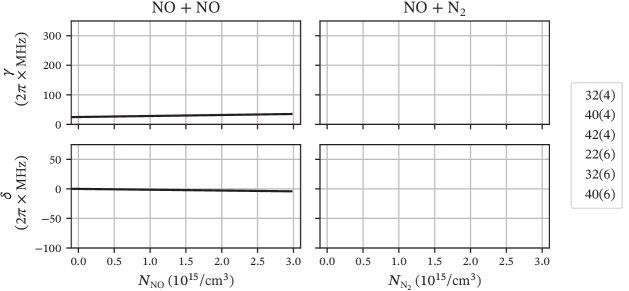
Figure 3: FWHM $\gamma$ and relative shift $\delta$ for NO being subject to an increasing density $N$ of the background gas, either NO itself on the left or N₂ on the right. Plotted are the results for different principle quantum numbers $n$ and rotational quantum numbers $N^{+}$ of the ionic core (Hund’s case (d)), and the notation $n(N^{+})$ is used in the legend. The relative shift is moved such that the first measurement points are referenced to zero. The black line indicates possible contributions by effects on the $\text{H}\,{}^{2}\Sigma^{+}$–state as explained in the text.

III Results

For the evaluation of our measurements we start by calculating the frequency axis out of the time axis by using the known free–spectral range of the Rydberg laser’s transfer cavity. The peak distances are fitted against the position in time by using a third–order polynomial function. The voltage signal is smoothed by a filter such that a following data reduction is not affecting the quality. Note that the TIA converts and amplifies from current to voltage, and the signal we process here is the lock–in amplifiers output signal. For each trace the most dominant center peak of the high–$l$–manifold, i.e. the peak not affected by the Stark effect, and the left and right of it are fitted using individual Voigt functions of the form

$$f(\omega)=A\cdot f_{\text{Voigt}}\left(\omega,\omega_{0},\gamma_{\text{L}},\sigma\right)+\mathcal{P}_{3}(\omega)\quad,$$ (1)

where $\mathcal{P}_{3}(\omega)$ is a polynomial function of third order to account for the baseline, $A$ is the amplitude, $\gamma_{\text{L}}$ is the Lorentzian part of the full width at half maximum (FWHM), $\gamma_{\text{G}}=2\sqrt{2\log(2)}\sigma$ is the Gaussian part of the FWHM, and $\omega_{0}$ is the center position relevant to extract the shift. The Voigt function $f_{\text{Voigt}}$ is normalized to its amplitude. Special care is taken for the polynomial bounds such that the effects on the parameters of interest are negligible. While we only look at the center peak, the side peaks are fitted for consistency checking. We use

$$\gamma\approx\frac{1}{2}\left[1.0692\frac{\gamma_{\text{L}}}{2}+\sqrt{0.86639\left(\frac{\gamma_{\text{L}}}{2}\right)^{2}+4\gamma_{\text{G}}^{2}}\right]$$ (2)

from [24] to calculate the overall FWHM $\gamma$. Note that we would expect a Lorentzian shape due to the homogeneity of collisional broadening. However, as we will see later, additional contributions such as the small pressure shift of the second transition $\text{H}\,{}^{2}\Sigma^{+}\leftarrow\text{A}\,{}^{2}\Sigma^{+}$ are present in our experiment. During the evaluation we verified that a fit with a Voigt function suits our results best. In figure 3 we show our results for the FWHM $\gamma$ and the relative shift $\delta$.

We start by considering the pressure broadening of the selected Rydberg state $n(N^{+})$. In general, several mechanisms contribute to the broadening of the linewidth $\gamma$ of the Rydberg line, namely residual Doppler broadening, power broadening, transit-time broadening and broadening due to polarization effects. In the case of NO it is hard to give numbers to Doppler broadening, power broadening or polarization effects as literature values cannot be easily determined. However, in the case of Doppler broadening, a lower bound can be given by taking the linewidth of $2\pi\times$15\text{\,}\mathrm{MHz}$$ as seen in [18] of the UV transition and accounting for $k$–vector mismatch, which yields around $2\pi\times$8\text{\,}\mathrm{MHz}$$. Additionally, the linear behavior shown in figure 3 suggests that collisional effects are dominating. In the case of collisions of NO with NO or NO with N₂ the broadening is basically the same with increasing density of the perturber. N₂ and NO differ only by a single electron when considering the orbital structure. For NO only one of the two levels of the $\pi^{*}_{2\text{p}}$ is occupied with a single electron [25], whereas for N₂ all are empty. This makes the broadening contributions similar. On top the Boltzmann distribution, describing the population of the rotational levels for a diatomic molecule, is given by Herzberg as [26]

$$P(J)=hcB_{v}\frac{2J+1}{k_{\text{B}}T}\exp\left[-hc\frac{B_{v}J(J+1)}{k_{\text{B}}T}\right]\quad,$$ (3)

where $P(J)$ is the population probability of having a rotational state with total angular momentum $J$ at temperature $T$ occupied. The Planck constant is denoted by $h$, $k_{\text{B}}$ is the Boltzmann constant and $c$ is the speed of light. For NO the rotational constant $B_{v}$, as given in [22] yields, that rotational levels from $J=0.5$ to $J=19.5$ have a population probability above $1\text{\,}\mathrm{\char 37\relax}$, suggesting significant contribution to the broadening. In contrast, any alkali being a simple atom, lacks these additional contributions [15, 16]. Consider the relative shift $\delta$ next. Based on Fermi’s work [14] elastic collisions between the Rydberg electron and perturbing atoms or molecules lead to a frequency shift $\delta$ of

$$\delta=\frac{\hbar}{m_{e}}a\cdot N,$$ (4)

where $N$ denotes the density, $m_{e}$ is the electronic mass, $a$ is the scattering length, and $\hbar$ is the reduced Planck constant. In the case of NO perturbed by NO a red shift can be seen. In the case of perturbations by N₂ the considered density range indicates a slight shift to the blue less than the scattering of the measured values. Inelastic collisions do not lead to a phase shift in the Rydberg electron’s wavefunction but change the state of the Rydberg atom or molecule itself. While both collision types may occur, this gives an indication in likeliness. For a rare gas such elastic collisions are expected due to the closed–shell structure [15, 16]. Interestingly our results show similar results for perturbations of NO with NO itself. A possible explanation for this is that NO has a degenerate level in the $\pi^{*}_{2\text{p}}$ available, suggesting that elastic collisions may occur despite the rotational and vibrational freedom. This explanation is supported by the fact that the molecule NO^-, though short-lived, even exists in biological processes [27]. However, when looking at N₂, a similar argument could be made. From our measurements it is undecidable, if a particular collision type is dominating in the case of perturbations by N₂.

Similar measurements have been performed without the Rydberg laser to investigate the effect on the $\text{H}\,{}^{2}\Sigma^{+}$–state. While a broadening and shift could be observed, its contribution is negligible. We show this in an added black line to figure 3, where we scaled a linear fit to these measurements by the wavevector mismatch as was done in equation (4) in [28]:

$$\frac{k_{1}-k_{2}-k_{3}}{k_{1}-k_{2}}\approx$0.53$$$ (5)

The resulting scaled functions are

$$\gamma(N)/2\pi \approx$3.41\text{\cdot}{10}^{15}\text{\,}\mathrm{MHz}\text{\,}{\mathrm{cm}}^{3}$\cdot N+$24.87\text{\,}\mathrm{MHz}$,$$ (6a)

$$\delta(N)/2\pi \approx$-1.38\text{\,}\mathrm{MHz}\text{\,}{\mathrm{cm}}^{3}$\cdot N.$$ (6b)

While we do not have to consider this contribution for the overall behavior, the contribution by the intermediate transition $\text{H}\,{}^{2}\Sigma^{+}\leftarrow\text{A}\,{}^{2}\Sigma^{+}$ partly explains the necessity of using a Voigt function for fitting rather than a Lorentzian. Further inhomogeneities might arise from the already introduced available degrees of freedom in a molecule.

In a next step we compare our results with results from the literature. Füchtbauer et al. [15] and Weber et al. [16] both investigated the shift of spectroscopic lines of alkalis being subject to a perturbing rare gas. In Füchtbauer’s experiment the alkalis sodium and potassium were subject to collisions with three different rare gases, helium, neon and argon. In Weber’s experiment the rubidium $n$D and $n$S transitions were shifted by helium, xenon and argon. In contrast to Füchtbauer, Weber was able to analyze the broadening as well. Comparison is easiest when using the broadening rate $\gamma/N$ and shift rate $\delta/N$ as introduced by Weber. In table 1 we list some exemplary literature values. We give both values extracted from a fit to the data plotted in figure 3 and listed in table 2. The fit of the shift against the density is done by a linear function in accordance with equation 4.

Table 1: Selected examplary values at different principle quantum numbers $n$ of Rydberg states in alkalis from measurements taken by Weber et al. [16] and Füchtbauer et al. [15]. For measurements by Füchtbauer, Rydberg states of potassium (K) are perturbed by argon (Ar), and for measurements by Weber we take their values of rubidium (Rb) Rydberg $n$S–states perturbed by argon. In the case of Füchtbauer we calculated the rates by using the ideal gas law.

	Füchtbauer et al.	Weber et al.
	K + Ar	($n$S) Rb + Ar
$n$	$\delta/N$	$\delta/N$	$\gamma/N$
21	-10.97	-4.76	1.46
23	-10.94	-4.94	1.56
25	-11.34	-5.02	1.66
27		-5	1.77
29		-5	1.8
33		-5.16	1.36
35		-5.04	1.36

Table 2: Broadening and shift rate, $\gamma/N$ and $\delta/N$, extracted from a fit to the measurement results shown in figure 3. The fit functions are explained in the text. The unit for all values is $10^{15}\cdot 2\pi\times\text{MHz}\,\text{cm}^{3}$. The main error contribution to the values is the absolute pressure uncertainty of $30\text{\,}\mathrm{\char 37\relax}$ of the used gauges.

State	NO + NO		NO + N2
$n(N^{+})$	$\gamma/N$	$\delta/N$	$\gamma/N$	$\delta/N$
$32(4)$	$130(39)$	$-28(8)$	$55(16)$	$2.5(0.8)$
$40(4)$	$106(32)$	$-25(7)$	$40(12)$	$5.7(1.7)$
$42(4)$	$91(27)$	$-21(6)$	$40(12)$	$1.9(0.6)$
$22(6)$	$75(23)$	$-27(8)$	$92(28)$	$5.2(1.6)$
$32(6)$	$148(44)$	$-14(4)$	$49(15)$	$8.2(2.5)$
$40(6)$	$103(31)$	$-23(7)$	$61(18)$	$0.89(0.27)$

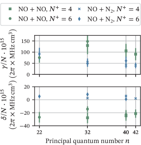
Figure 4: Broadening rate $\gamma/N$ and shift rate $\delta/N$ of the perturbation of Rydberg states in NO. We explain the high broadening rate in comparison to alkalis as seen in [15, 16] by the additional degrees of freedom in a molecule. Some exemplary alkali values are given in 1. An uncertainty of $30\text{\,}\mathrm{\char 37\relax}$ in the measured pressure is indicated by error bars. For some measurement points the marker covers the error bar. Within the error the values are constant, which is expected when compared to alkalis. The individual values are given in table 2.

For the broadening we use

$$f_{\text{fit}}(N)=\sqrt{\text{offset}^{2}+\left(\frac{\gamma}{N}\cdot N\right)^{2}}\quad,$$ (7)

as a fit function to account for the additional broadening contribution in the low densities by an offset. We give an error estimate to all fitted values as well. The largest contribution to our errors has its origin in the absolute pressure given by our pressure gauges (Pfeiffer PKR 251) and amounts to $30\text{\,}\mathrm{\char 37\relax}$. In contrast, as seen in [18], the uncertainty of our frequency axis, $2\pi\times$2.5\text{\,}\mathrm{MHz}$$, can in this case be neglected. As such the error given is based solely on the pressure uncertainty. In comparison with [16, 15] our broadening rate $\gamma/N$ is several times higher than their values. The shift rate $\delta/N$ deviates by one order of magnitude, when comparing measurements of NO and alkalis, which indicates that additional processes are present in molecules.

IV Summary

We showed the collisional shift and broadening of Rydberg states in NO with increasing density of two background gases. The detection of the Rydberg states was realized by an electrical readout of the current generated by free charges resulting from collisions. The linear shift of elastic collisions can be understood as introduced by Fermi [14].

The measurement was either performed on NO being perturbed by itself or N₂. Comparison to literature values [15, 16] of the experiment was achieved by extracting the broadening rate $\gamma/N$ and shift rate $\delta/N$ using fits to our experimental data. The analysis showed that for perturbations by NO elastic collisions dominate, yet it is impossible to give such a clear statement in the case of collisions with N₂. In any case our rates are orders of magnitude higher when compared to measurements done in alkalis. We attribute this to the additional degrees of freedom in NO.

The overall project’s goal is to realize a breath-gas sensor for NO in the context of a possible medical application. In this context, the main effect to consider is the broadening rate, since it is larger than the shift rate.

References

- Arnold et al. [1977] W. P. Arnold, C. K. Mittal, S. Katsuki, and F. Murad, Nitric oxide activates guanylate cyclase and increases guanosine 3':5'-cyclic monophosphate levels in various tissue preparations, Proceedings of the National Academy of Sciences 74, 3203 (1977).
- Furchgott and Zawadzki [1980] R. F. Furchgott and J. V. Zawadzki, The obligatory role of endothelial cells in the relaxation of arterial smooth muscle by acetylcholine, Nature 288, 373 (1980).
- Ignarro et al. [1987] L. J. Ignarro, G. M. Buga, K. S. Wood, R. E. Byrns, and G. Chaudhuri, Endothelium-derived relaxing factor produced and released from artery and vein is nitric oxide., Proceedings of the National Academy of Sciences 84, 9265 (1987).
- The Nobel Foundation [1998] The Nobel Foundation, The nobel prize in physiology or medicine (1998).
- Ignarro [2018] L. J. Ignarro, Nitric oxide is not just blowing in the wind, British Journal of Pharmacology 176, 131 (2018).
- Haklar et al. [2001] G. Haklar, E. Sayin-Özveri, M. Yüksel, A. Aktan, and A. Yalçin, Different kinds of reactive oxygen and nitrogen species were detected in colon and breast tumors, Cancer Letters 165, 219 (2001).
- [7] S. K. (Choudhari), G. Sridharan, A. Gadbail, and V. Poornima, Nitric oxide and oral cancer: A review, Oral Oncology 48, 475 (2012).
- Xu et al. [2002] W. Xu, L. Z. Liu, M. Loizidou, M. Ahmed, and I. G. Charles, The role of nitric oxide in cancer, Cell Research 12, 311 (2002).
- Khan et al. [2020] F. H. Khan, E. Dervan, D. D. Bhattacharyya, J. D. McAuliffe, K. M. Miranda, and S. A. Glynn, The role of nitric oxide in cancer: Master regulator or NOt?, International Journal of Molecular Sciences 21, 9393 (2020).
- Thomas et al. [2008] D. D. Thomas, L. A. Ridnour, J. S. Isenberg, W. Flores-Santana, C. H. Switzer, S. Donzelli, P. Hussain, C. Vecoli, N. Paolocci, S. Ambs, C. A. Colton, C. C. Harris, D. D. Roberts, and D. A. Wink, The chemical biology of nitric oxide: Implications in cellular signaling, Free Radical Biology and Medicine 45, 18 (2008).
- Gustafsson et al. [1991] L. Gustafsson, A. Leone, M. Persson, N. Wiklund, and S. Moncada, Endogenous nitric oxide is present in the exhaled air of rabbits, guinea pigs and humans, Biochemical and Biophysical Research Communications 181, 852 (1991).
- American Thoracic Society and European Respiratory Society [2005] American Thoracic Society and European Respiratory Society, ATS/ERS recommendations for standardized procedures for the online and offline measurement of exhaled lower respiratory nitric oxide and nasal nitric oxide, 2005, American Journal of Respiratory and Critical Care Medicine 171, 912 (2005).
- Schmidt et al. [2018] J. Schmidt, M. Fiedler, R. Albrecht, D. Djekic, P. Schalberger, H. Baur, R. Löw, N. Fruehauf, T. Pfau, J. Anders, E. R. Grant, and H. Kübler, Proof of concept for an optogalvanic gas sensor for NO based on rydberg excitations, Applied Physics Letters 113, 10.1063/1.5024321 (2018).
- Fermi [1934] E. Fermi, Sopra lo spostamento per pressione delle righe elevate delle serie spettrali, Il Nuovo Cimento 11, 157 (1934).
- Füchtbauer et al. [1934] C. Füchtbauer, P. Schulz, and A. F. Brandt, Verschiebung von hohen Serienlinien des Natriums und Kaliums durch Fremdgase, Berechnung der Wirkungsquerschnitte von E delgasen gegen sehr langsame Elektronen, Zeitschrift für Physik 90, 403 (1934).
- Weber and Niemax [1982] K. H. Weber and K. Niemax, Impact broadening and shift of Rb nS and nD levels by noble gases, Zeitschrift für Physik A Atoms and Nuclei 307, 13 (1982).
- González-Férez et al. [2021] R. González-Férez, J. Shertzer, and H. Sadeghpour, Ultralong-range rydberg bimolecules, Physical Review Letters 126, 10.1103/physrevlett.126.043401 (2021).
- Kaspar et al. [2022] P. Kaspar, F. Munkes, P. Neufeld, L. Ebel, Y. Schellander, R. Löw, T. Pfau, and H. Kübler, Phys. Rev. A 106, 062816 (2022).
- Neuhaus et al. [2017] L. Neuhaus, R. Metzdorff, S. Chua, T. Jacqmin, T. Briant, A. Heidmann, P.-F. Cohadon, and S. Deléglise, Pyrpl (python red pitaya lockbox) — an open-source software package for fpga-controlled quantum optics experiments, in 2017 Conference on Lasers and Electro-Optics Europe & European Quantum Electronics Conference (CLEO/Europe-EQEC) (2017) pp. 1–1.
- Mäusezahl et al. [tion] M. Mäusezahl, F. Munkes, and R. Löw, Tutorial on locking techniques and the manufacturing of vapor cells for spectroscopy (in preparation).
- Western [2017] C. M. Western, PGOPHER: A program for simulating rotational, vibrational and electronic spectra, Journal of Quantitative Spectroscopy and Radiative Transfer 186, 221 (2017).
- Danielak et al. [1997] J. Danielak, U. Domin, R. Ke, M. Rytel, and M. Zachwieja, Reinvestigation of the emission band system ( – ) of the no molecule, Journal of Molecular Spectroscopy 181, 394 (1997).
- Ogi et al. [2000] Y. Ogi, M. Takahashi, K. Tsukiyama, and R. Bersohn, Laser-induced amplified spontaneous emission from the 3d and nf rydberg states of NO, Chemical Physics 255, 379 (2000).
- Olivero and Longbothum [1977] J. Olivero and R. Longbothum, Empirical fits to the voigt line width: A brief review, Journal of Quantitative Spectroscopy and Radiative Transfer 17, 233 (1977).
- Schulz-Weiling [2017] M. Schulz-Weiling, Ultracold Molecular Plasma, Ph.D. thesis (2017).
- Herzberg [1950] G. Herzberg, Spectra of Diatomic Molecules, second edition ed., Molecular Spectra and Molecular Structure, Vol. 1 (D. Van Nostrand Company, Inc., 1950).
- Hughes [1999] M. N. Hughes, Relationships between nitric oxide, nitroxyl ion, nitrosonium cation and peroxynitrite, Biochimica et Biophysica Acta (BBA) - Bioenergetics 1411, 263 (1999).
- Kübler and Shaffer [2018] H. Kübler and J. P. Shaffer, A read-out enhancement for microwave electric field sensing with rydberg atoms, in Quantum Technologies 2018, edited by A. J. Shields, J. Stuhler, and M. J. Padgett (SPIE, 2018).