TeV neutrinos and hard X-rays from relativistic reconnection in the corona of NGC 1068
Abstract
The recent discovery of astrophysical neutrinos from the Seyfert galaxy NGC 1068 suggests the presence of non-thermal protons within a compact “coronal” region close to the central black hole. The acceleration mechanism of these non-thermal protons remains elusive. We show that a large-scale magnetic reconnection layer, of the order of a few gravitational radii, may provide such a mechanism. In such a scenario, rough energy equipartition between magnetic fields, X-ray photons, and non-thermal protons is established in the reconnection region. Motivated by recent three-dimensional particle-in-cell simulations of relativistic reconnection, we assume that the spectrum of accelerated protons is a broken power law, with the break energy being constrained by energy conservation (i.e., the energy density of accelerated protons is at most comparable to the magnetic energy density). The proton spectrum is below the break, and above the break, with IceCube neutrino observations suggesting . Protons above the break lose most of their energy within the reconnection layer via photohadronic collisions with the coronal X-rays, producing a neutrino signal in good agreement with the recent observations. Gamma-rays injected in photohadronic collisions are cascaded to lower energies, sustaining the population of electron-positron pairs that makes the corona moderately Compton thick.
1 Introduction
Active galactic nuclei (AGN) are among the most energetic sources in the Universe. They are powered by accreting supermassive black holes (SMBHs), and their main emission features (see, e.g., Marconi et al., 2004; Ghisellini, 2013; Padovani et al., 2017) can be summarized as: (i) an optical-ultraviolet thermal component, often referred to as the “big blue bump”, which is produced by the accretion disk; (ii) a second thermal component radiated by the dusty torus in the infrared; (iii) an X-ray power law extending up to keV, which is believed to be associated with the AGN “coronal” region.
The coronal region of AGN has been proposed as a production site of multi-messenger emission since the late seventies (Berezinsky, 1977; Silberberg & Shapiro, 1979; Eichler, 1979). Very recently, the IceCube collaboration has reported compelling evidence of a high-energy neutrino flux from NGC 1068 (Aartsen et al., 2020; Abbasi et al., 2022), a nearby Seyfert II galaxy located at a distance of 10.1 Mpc (Tully et al., 2008, and Padovani et al., in prep.). This neutrino flux has been measured with a significance of 4.2 in the energy band 1.5–15 TeV, showing a soft neutrino spectrum . A comparable TeV gamma-ray flux, which would be expected for an optically thin source, is not observed, with stringent upper limits set by the MAGIC telescope (Acciari et al., 2019). This suggests that the neutrino source must be located close to the AGN innermost regions, where the dense optical and X-ray radiation would reprocess gamma rays to lower energies (Berezinsky & Ginzburg, 1981). Thus, the GeV gamma rays observed by Fermi-LAT (Abdo et al., 2010) are hard to explain within the coronal model, and are generally attributed to a different region, e.g., the weak jet observed in the core of the galaxy (Lenain et al., 2010), the circumnuclear starburst (Yoast-Hull et al., 2014; Ambrosone et al., 2021; Eichmann et al., 2022), a large scale AGN-driven outflow (Lamastra et al., 2016), a combination of successful and failed line-driven wind (Inoue et al., 2022), or an ultra-fast outflow (Peretti et al., 2023).
Neutrino emission from AGN cores directly points to the presence of a relativistic hadronic population, but the specific particle acceleration mechanism at work remains an open question. Inoue et al. (2020) and Murase et al. (2020) provided the first phenomenological modeling of NGC 1068, prescribing that protons are energized via diffusive shock acceleration (DSA) or stochastic acceleration, respectively. Both models highlighted the importance of Bethe-Heitler (BH) interactions on optical photons as the main mechanism limiting proton acceleration. Kheirandish et al. (2021) discussed magnetic reconnection as a potential mechanism for proton acceleration in a weakly magnetized corona. Assuming a proton power-law spectrum with slope , they computed the neutrino emission from and inelastic collisions, and applied their analysis to NGC 1068. Recently, Murase (2022) provided model-independent multi-messenger constraints on the acceleration processes, as well as on the production mechanism of high-energy neutrinos in AGN coronae. This study highlighted the importance of the electromagnetic cascade for reprocessing the GeV-TeV gamma rays into the MeV band.
The aim of this Letter is to explore the role of reconnection in magnetically-dominated plasmas for powering the X-ray and neutrino emission in AGN coronae. In this scenario, rough energy equipartition between magnetic fields, X-ray radiation, and relativistic protons is established in the reconnection region. Motivated by recent three-dimensional particle-in-cell (PIC) simulations of relativistic reconnection (Zhang et al., 2021, 2023; Chernoglazov et al., 2023), we assume that the spectrum of accelerated protons is a broken power law, with the break energy being constrained by energy conservation (i.e., the energy density of accelerated protons is at most comparable to the magnetic energy density)111As shown below, the break energy is well below the maximum proton energy achievable in reconnection.. The proton spectrum is hard below the break (slope around ), whereas it is softer above the break, which could explain the soft neutrino spectrum of NGC 1068. Our model has only two free parameters, namely the size of the reconnection region, and the number density of non-thermal protons in the coronal region, which directly determines . All other parameters can be either inferred by observations or benchmarked with PIC simulations.
In this Letter we demonstrate that the neutrino emission expected from relativistic reconnection in the coronal region of NGC 1068 is consistent with IceCube observations, and we show that the peak neutrino luminosity scales quadratically with the X-ray luminosity and inversely proportional to the black hole mass. For large X-ray luminosities, protons cool so fast that they lose most of their energy inside the reconnection layer, which effectively becomes a calorimeter: in this regime, the scaling saturates into a linear proportionality with the X-ray luminosity, independently of the black hole mass and layer size. We find that Bethe-Heitler and photohadronic interactions initiate an electromagnetic cascade that ultimately establishes and maintains a population of electron-positron pairs, which naturally makes the corona moderately optically thick for the Comptonization of low-energy photons up to the hard X-ray band.
2 Properties of the reconnection layer
In this section we identify the main properties of the reconnection layer. Assuming that the hard X-ray flux comes from Comptonization within the reconnection layer, we can infer the electron number density, and also provide an estimate for the magnetic field strength in the reconnection layer.
We envision the formation of a reconnection layer in the vicinity of a black hole with mass . In order to maintain our conclusions as general as possible, we do not specify the exact origin and location of this reconnection layer. One possible scenario is the equatorial current sheet that naturally arises in the innermost region of magnetically-arrested disks (Avara et al., 2016; Dexter et al., 2020; Ripperda et al., 2020; Porth et al., 2021; Scepi et al., 2022; Nathanail et al., 2022; Ripperda et al., 2022). Another possibility is the reconnection layer adjacent to the jet boundary (Nathanail et al., 2020; Chashkina et al., 2021; Davelaar et al., 2023), or beyond the Y-point of field lines connected to both the disk and the black hole (El Mellah et al., 2022, 2023). Regardless of its specific origin, the presence of this macroscopic reconnection layer facilitates the rapid conversion of the available magnetic energy into particle energy. A fraction of this energy can be reprocessed into hard X-rays. Traditionally, this has been associated with the Comptonization of low-energy photons from the accretion disk by a population of hot coronal electrons with keV temperature (Sunyaev & Truemper, 1979; Sunyaev & Titarchuk, 1980; Haardt & Maraschi, 1991, 1993). More recently, alternative scenarios have been proposed, in which X-rays are Comptonized by the bulk motions of a turbulent plasma (Groselj et al., 2023) or by the trans-relativistic bulk motions of the stochastic chain of reconnection plasmoids (Beloborodov, 2017; Sironi & Beloborodov, 2020; Sridhar et al., 2021, 2023). We refrain from adopting a specific scenario to describe the X-ray coronal emission of NGC 1068, and use instead some general considerations applicable to accreting systems with magnetically-powered hard X-ray emission.
We consider a reconnection layer of length which we scale with the black hole gravitational radius . The cross-sectional area of the “upstream” plasma flowing into the reconnection layer is estimated as . The characteristic thickness of the layer of reconnected plasma (the reconnection “downstream”) is determined by the size of the largest plasmoids, which can be estimated as . Here, represents the plasma inflow speed into the reconnection layer normalized to the speed of light. Its value is also representative of the ratio between the reconnection electric field and the reconnecting magnetic field . The choice of (Comisso & Bhattacharjee, 2016; Cassak et al., 2017) is appropriate for the collisionless relativistic regime in which the magnetization exceeds unity, where is the plasma mass density. As shown below, this is indeed our regime of interest.
In both X-ray binaries (Reig et al., 2018; Malzac et al., 2001; Zdziarski, 2000) and luminous AGN (Wilkins & Gallo, 2015; Petrucci et al., 2020; Tripathi & Dewangan, 2022), the shape of the X-ray spectrum suggests that the optical depth for Comptonization is moderate (i.e. ). Motivated by radiative PIC simulations (Sridhar et al., 2021, 2023), we use the condition , where is the Thomson cross section and is the cold pair number density (henceforth, the electron density), to infer
| (1) |
where .
The strength of the reconnecting field can be obtained by assuming that the coronal hard X-ray emission comes from dissipation of magnetic energy in reconnection, as argued in Beloborodov (2017). We assume that a fraction of the Poynting flux crossing the reconnection plane is dissipated into Comptonized X-rays (the rest stays in electromagnetic fields, see, e.g., Sironi et al. 2015), namely
| (2) |
Noting that the X-ray flux is related to the intrinsic X-ray luminosity as , where the factor of two accounts for emission from both sides of the layer, the magnetic energy density is written as
| (3) |
where is the bolometric intrinsic X-ray luminosity of NGC 1068. This implies a magnetic field
| (4) |
Taking the pair number density from the optical depth argument presented above, we can estimate the magnetization of the system as
| (5) |
where we have assumed that ions do not appreciably contribute to the mass density, namely the proton number density is . As we discuss in Section 3.4, this condition is supported by neutrino observations. As anticipated above, reconnection in a system with is identified as “relativistic”.
3 Relativistic protons in the reconnection layer
In this section, we first discuss the physics of proton acceleration in relativistic reconnection, and the expected proton spectrum. We then describe the hierarchy of time scales (or equivalently of energy scales), accounting for proton acceleration, escape from the reconnection layer, and various cooling losses. We determine the steady-state proton spectrum and use it to predict the TeV neutrino flux.
3.1 Spectrum of accelerated protons
Our understanding of the physics of particle acceleration in relativistic reconnection has greatly advanced in recent years thanks to first-principles particle-in-cell (PIC) simulations (Werner & Uzdensky, 2017; Zhang et al., 2021, 2023; Chernoglazov et al., 2023). Motivated by 3D PIC simulations of reconnection in the relativistic regime, we assume that, in the absence of proton cooling losses: (i) protons are accelerated linearly in time with an energization rate of approximately , (ii) nearly all protons flowing into the reconnection layer are injected into the acceleration process, and (iii) the proton spectrum can be modeled as a broken power law with below some break energy , and with above the break energy, up to a cutoff energy corresponding to the maximum energy that protons can attain in the absence of cooling losses.
The value of the post-break slope depends on various physical conditions, including the strength of the “guide” field (i.e., the non-reconnecting component orthogonal to the oppositely-directed fields). In fact, Werner & Uzdensky (2017) used 3D PIC simulations to show that, as the guide field strength increases from to , the high-energy spectral slope increases from to (so, the spectrum gets steeper). In the following, we deduce the post-break slope from IceCube neutrino observations, which suggest .
The characteristic energy at the spectral break is associated with the so-called proton magnetization , such that the break energy is of order . This is equivalent to stating that the energy density in the non-thermal proton population, , is comparable to the magnetic energy density, . We will later show that TeV is the ballpark value for the break energy needed to explain the IceCube neutrino observations.
3.2 Proton acceleration, escape and cooling
Zhang et al. (2021) and Zhang et al. (2023) elucidated the physics of particle acceleration in relativistic 3D reconnection. They showed that particles gain most of their energy in the inflow (upstream) region, while meandering between the two sides of the reconnection layer. Here, the timescale for proton acceleration is of the order of
| (6) |
Particles leave the region of active acceleration when they get captured by one of the flux ropes/plasmoids of reconnected plasma. At that point, they are no longer actively accelerated, and they either advect out of the system (on a timescale ), or they cool due to radiative losses. In the discussion that follows, we focus on the proton spectrum in the downstream region of reconnected plasma, assuming—based on PIC simulations (Werner & Uzdensky, 2017; Zhang et al., 2021, 2023; Chernoglazov et al., 2023)—that the prior phase of active energization injects a broken power-law spectrum scaling as below the break and as above the break. Protons escape/advect out of the reconnection region on a typical timescale
| (7) |
The dominant channel of proton energy loss is photohadronic () inelastic scattering on the X-ray photon field; we discuss in App. A additional cooling processes which turn out to be subdominant. To compute the cooling rate we parameterize the X-ray coronal emission as follows. The X-ray energy density is given by . In the optically thick regime, we expect this estimate to be revised by a corrective factor proportional to , but since we neglect the exact numerical factors in what follows. Motivated by spectral modeling of NGC 1068 (Bauer et al., 2015; Marinucci et al., 2016), we adopt a power-law spectrum of photon index between eV and keV,
| (8) |
The frequency range covered by the coronal spectrum is consistent with a scenario in which photons are initially injected in the optical-ultraviolet (OUV) band from the accretion disk, typically at energies even below eV, and subsequently undergo Comptonization in the corona up to keV. We emphasize though that the X-ray spectrum below about keV is not motivated by observations; on the other hand, as we discuss in more detail in Sec. 3.3, a different value of would not alter our results.
We assume an effective cross section that is constant in energy, b, for interaction energies above the center-of-mass energy threshold (in units of ), where is the total cross section, and is the proton inelasticity (Atoyan & Dermer, 2003; Dermer & Atoyan, 2003). Using the X-ray spectrum in Eq. 8, we estimate the energy-loss timescale as
for proton energies , which is defined as
| (10) |
In contrast, for the cooling timescale flattens to the asymptotic energy-independent value
since the scattering does not happen anymore at threshold for pion production, and becomes dominated by multi-pion interactions with the whole X-ray spectrum.
Another relevant energy scale is obtained by equating the cooling timescale with the escape/advection timescale
| (12) |
Above , protons cool much faster than they can escape the reconnection layer, and therefore lose most of their energy while being inside of it.
The maximum energy to which protons can be accelerated is set by the equality between the acceleration and the dominant energy-loss timescale. At very high energies, this can either be synchrotron (estimated in App. A) or , yielding (first and second term in the square bracket, respectively)
| (13) | |||
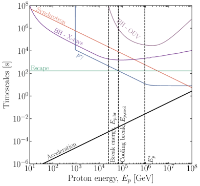
Fig. 1 collects the energy-dependent timescales we have introduced, for a benchmark choice of parameters representative of the likely conditions in NGC 1068 (see Sec. 3.6). We also show the synchrotron energy-loss timescale, and the BH energy-loss timescales due to X-ray and OUV photons separately, as discussed in App. A. We can grasp directly the main features discussed in the text: the acceleration timescale is much faster than all the other timescales up to hundreds of PeV. However, protons cool faster than the escape timescale, due to interactions, already very close to the break energy.
3.3 Steady-state proton spectrum
Here we consider the proton spectrum in the downstream region of reconnected plasma, assuming that the prior phase of active acceleration in the upstream injects a broken power law scaling as below the break and as above the break. When accounting for cooling losses, the steady-state proton spectrum will be composed of several power-law segments that depend on the hierarchy of the proton energy scales. For , as shown in Fig. 1, we expect
| (14) |
Notice that the break at , which is determined by the lower energy of the X-ray target , is typically much above the peak of the proton spectrum, and therefore does not impact the neutrino production close to the peak. Therefore, a lower value for would not significantly affect our results.
The overall normalization of the proton spectrum is determined by the condition of near-equipartition between magnetic field energy density and proton energy density. Specifically, we normalize the spectrum by assuming that the proton energy density is . In the absence of proton cooling losses, PIC simulations indicate that (French et al., 2023; Totorica et al., 2023; Comisso & Jiang, 2023). In what follows, we consider the special case where protons that carry most of the energy (i.e., those at ) are marginally fast-cooling, namely , and use as a typical value. In App. B, we generalize our results to the fast-cooling regime where .
If we take the energy hierarchy , with post-break slope of (motivated by the neutrino observations), we can compute the total proton number density,
| (15) | |||||
where we have replaced the square bracket by its typical order of magnitude value for TeV (i.e. typical value needed to reproduce the IceCube neutrino measurements). Eq. (15) confirms our initial assumption that , see Eq. (1). Charge neutrality therefore requires the largest part of the lepton population in the coronal region to be made of electron-positron pairs.
3.4 Neutrino emission
Photohadronic collisions inject charged pions, which subsequently decay to neutrinos. We estimate the production rate of neutrinos and anti-neutrinos of all flavors as
| (16) |
where is the rate of neutrino production differential in neutrino energy, is the volume of the reconnection region, and the factor is the fraction of proton energy converted to neutrinos. For interactions at -resonance , while for multi-pion interactions . For the target X-ray spectrum we are considering, using the two-bin parameterization for the interaction rate of Dermer & Atoyan (2003), we find that around a reasonable approximation is . We assume here that each neutrino carries on average an energy .
Since for , the neutrino spectrum is hardened by one power of energy as compared to the proton spectrum, whereas it has the same slope as the proton spectrum for . Taking the post-break proton slope to be as in Eq. 14, we expect a broken power law with for ; for ; and for (since the proton spectrum is steepened by photohadronic losses to ), see also Eq. 14. Thus, for our benchmark value of the post-break proton slope, the neutrino spectrum is consistent with IceCube observations. The peak value of , which lies in the energy range , is
| (17) | |||
For , this is comparable with the required luminosity needed to explain the IceCube flux, provided that is in the range TeV.
3.5 Proton-mediated pair enrichment
So far, we have left unspecified the origin of the leptonic population, whose number density we can infer from the Compton opacity. A thrilling possibility is that the proton population itself is responsible for maintaining a steady density of cold pairs in the coronal region. MeV photons, which are primarily emitted by Bethe-Heitler relativistic pairs (as we will show in Sec. 3.6), as well as cascaded from -produced gamma rays, inject pairs almost at rest after their attenuation. Because of the hadronic origin of MeV photons, we argue that the typical luminosity in the MeV band is comparable with the neutrino luminosity (see also Sec. 3.6). An order-of-magnitude estimate of the MeV photon energy density is
| (18) |
and their number density is . While this is only an order-of-magnitude estimate, it captures the expected scaling with the energy injected by hadrons; we validate it by comparing with our numerical simulations in Sec. 3.6. Finally, we can estimate the amount of pairs produced by MeV photon-photon attenuation as
| (19) | |||
For , the attenuation of MeV photons can therefore lead to a pair population that constitutes a sizeable fraction of the pair density inferred from the Compton opacity in Eq. 1. The above estimate should be taken as a lower limit, because we have only considered pair production via attenuation of MeV photons. We have not included, e.g., the contribution of relativistic pairs—produced in photohadronic interactions and from the attenuation of GeV-TeV gamma-ray photons—that cool down to Lorentz factors .
3.6 Neutrino emission from NGC 1068
We propose that reconnection-powered coronal neutrino emission is the dominant source of the neutrino flux observed by IceCube in coincidence with NGC 1068. Results are shown for a luminosity distance Mpc (see Tully et al., 2008, and Padovani et al., in prep.) and a black hole mass (see Greenhill et al., 1996, and Padovani et al., in prep.).
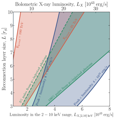
The first requirement is that the neutrino luminosity matches the observed all-flavor luminosity observed by IceCube. Assuming a peak neutrino energy of TeV, corresponding to a proton break energy TeV, the all-flavor neutrino luminosity is erg/s (based on the best-fit value and confidence region shown in Fig. 4 of Abbasi et al. (2022), after accounting for the difference in the luminosity distance used). The second requirement is that the neutrino spectrum observed by IceCube must be sufficiently soft, which can be accommodated in our model if the post-break proton slope is and simultaneously the cooling break is not much larger than the break energy . In this way, the neutrino spectrum is not hardened significantly by the energy dependence of the efficiency ( in Eq. 16), and the reconnection layer acts almost as a proton calorimeter. Therefore, our second constraint is that TeV. We take to lie between 25 TeV and 100 TeV (the fast-cooling case is discussed in more detail in App. B.)

Fig. 2 shows the regions of parameter space where both requirements are simultaneously satisfied, according to our analytical estimates. We consider as independent parameters the size of the reconnection layer and the X-ray luminosity in the keV range; while the latter is in principle observed, there is a relatively large uncertainty on its value erg/s (see Marinucci et al., 2016, and Padovani et al., in prep; we rescaled their luminosity to account for the different choice of luminosity distance), motivating the range chosen for the figure. The axis at the top shows the bolometric (0.1 keV – 100 keV) intrinsic X-ray luminosity , which we have used in our analytical estimates. We also show in green the region where the pairs produced by the attenuation of MeV photons according to Eq. 19 can contribute a sizable fraction, if not the entirety, of the pair population inferred from the Compton opacity argument. The allowed parameter space provides a coherent explanation for both the neutrino signal and the moderate optical depth of coronal regions.
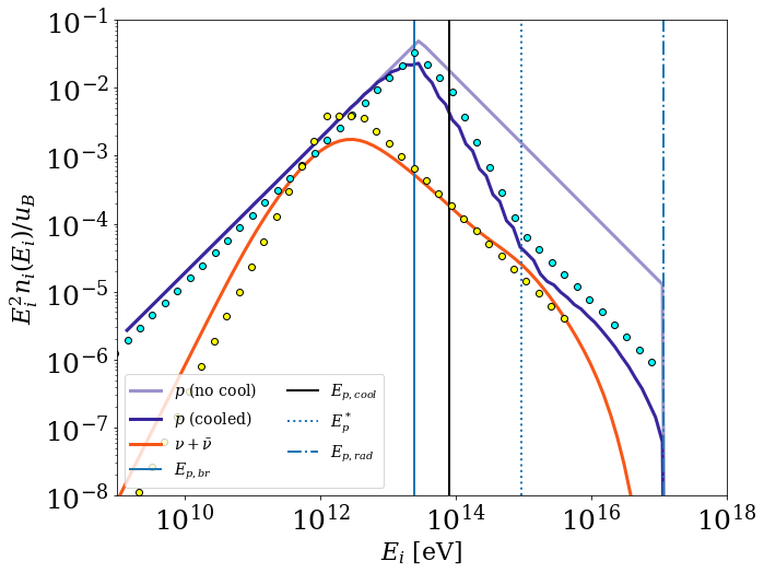
To confirm our analytical estimates, we have also performed numerical calculations of the neutrino and gamma-ray production within a spherical coronal region of size ; we describe in Appendices C and D the relation between the spherical geometry of our numerical calculations and the planar one used in our analytical estimates, as well as the main properties of the numerical code we used. We show the resulting neutrino spectral energy distribution in Fig. 3 (orange solid line), whose peak is in reasonable agreement with the analytical expectation (orange circle)222A comparison of the numerically-computed steady-state proton distribution with the analytical expression of Eq. 14 can be found in App. D.. Our calculations do not account for neutron-photon interactions; we have separately evaluated them numerically, finding that they can account for a increase in the neutrino flux shown in Fig. 3.
The large opacity to photon-photon pair production of the coronal region suppresses the gamma-ray spectrum at energies MeV, making it consistent with the observations. Synchrotron radiation of Bethe-Heitler pairs is an important source of MeV photons, which produce pairs with . Attenuation of more energetic photons arising from interactions leads to the production of relativistic secondary electrons and positrons, which cool down to within a dynamical time due to the strong synchrotron losses. As a result, attenuation of gamma-ray photons produced from photohadronic interactions provides another channel for injecting cold pairs in the system. With our numerical code, we find that the density of pairs resulting from the attenuation of hadronically-produced photons is cm-3, which leads to . This numerical value is also consistent with the analytical estimate computed for a spherical geometry, see Eq. C11.
We note that the radiative calculations we presented have some limitations. First, cold pairs are “passive” (i.e., non-emitting) particles in our code, since radiative processes of non-relativistic electrons (e.g., cyclotron radiation and Compton scattering) are not implemented. Second, we do not account for the energization of leptons due to magnetic reconnection or their synchrotron emission, which might be important for the low-energy end of the photon spectrum. For this reason, we only show the photon spectrum down to 1 eV, and consider the X-ray coronal emission given (i.e., no interaction between cold pairs and X-ray photons is considered).
4 Summary and Discussion
We propose that protons energized by magnetic reconnection in a highly magnetized, pair-dominated plasma interact with hard X-rays from the corona and produce the high-energy neutrinos observed by IceCube from the Seyfert galaxy NGC 1068. The key ingredient of this study—grounded on recent 3D PIC simulations of relativistic reconnection—is that the X-ray coronal emission, the energy density of reconnecting magnetic fields, and the relativistic proton population are all connected with each other.
If hard X-ray photons are produced via Comptonization of lower energy photons by pairs in the reconnection region, as previously proposed, then the energy density of up-scattered photons will be a fraction (of order ) of the energy density of reconnecting magnetic fields. Protons accelerated in the reconnection region will also carry a fraction of the magnetic energy density. To avoid an “energy crisis”, the hard proton spectrum established at low energies must soften (, with ) above a characteristic break energy . From the peak of the observed neutrino flux, we infer TeV. Under these conditions, the neutrino emission can be fully determined by only two parameters: the size of the reconnection region, and the X-ray luminosity of the corona (which is observationally constrained, but with large error bars).
In our scenario, the proton break energy happens to be just below the energy at which photohadronic cooling becomes faster than the proton escape/advection from the reconnection layer. This implies that most of the energy in the accelerated protons is lost to neutrinos and gamma rays. While the latter are not able to escape the optically-thick reconnection layer, and are cascaded down to lower energies, neutrinos carry away a significant fraction of the proton energy, explaining the relatively large flux observed by IceCube. Our scenario naturally leads to a robust scaling of the peak neutrino luminosity with black hole mass and X-ray luminosity, i.e., , which comes from the direct connection between X-ray, magnetic, and non-thermal proton energy density. In the case of fast-cooling, with , the scaling with becomes linear with no dependence on black hole mass and layer size, since the reconnection layer becomes calorimetric.
Intriguingly, we also find that the pair population induced by the cascade initiated by interactions and by the attenuation of Bethe-Heitler-produced MeV photons is comparable with the one inferred from the Compton optical thickness of the corona. Even though this result is not a strict requirement, i.e., the bulk of the pairs might have a different origin, it is a natural outcome of our model, at least for the parameters of NGC 1068. We are therefore prompted to speculate that the non-thermal proton population may play an important role also in maintaining the large lepton density in AGN coronae. A more thorough dynamic study of the interplay between protons and X-ray coronal photons is yet to be carried out.
Based on our findings, reconnection layers in AGN coronae are magnetically-dominated (i.e., the magnetic energy density is much larger than the plasma rest-mass energy density) and significantly pair-enriched, to the point that the upstream mass density is mostly contributed by electron-positron pairs. Equivalently, if the magnetization is normalized to the pair mass density, we have , where the “proton magnetization” is (see Eq. 15)
| (20) |
The low value of the proton number density (equivalently, the high ) seems to be somewhat needed for the observability of the neutrino signal. A much higher proton density would correspond to a much lower break energy (at fixed magnetic energy density), so the neutrino signal would peak in an energy range unobservable by IceCube.
Interestingly, the three scenarios presented in Section 2 for the formation of a large-scale coronal reconnection layer are likely consistent with a pair-dominated, proton-poor composition (in GRMHD simulations, the particle density in the layer is found to be dominated by artificially-injected density floors, rather than by the physical density of the initialized electron-proton torus)333This can also be the case for reconnection layers at the jet/wind boundary (Nathanail et al., 2020; Chashkina et al., 2021; Davelaar et al., 2023), if reconnection occurs because of jet field lines winding up onto themselves due to the underlying velocity shear, see Sironi et al. (2021).. To the best of our knowledge, 3D PIC simulations in this regime () have yet to properly quantify how the post-break proton slope depends on the guide field strength. Werner & Uzdensky 2017 demonstrated that the high-energy spectral slope is steeper for stronger guide fields—with for a guide field comparable to the reconnecting field—but their simulations adopted an electron-positron composition. If our observationally-motivated choice of is indeed to be attributed to a guide field comparable to the reconnecting field, then the reconnection layer at the jet boundary is the most likely scenario (e.g., Sironi et al., 2021). But in general, whether a relatively strong guide field is attained in the three scenarios presented in Section 2 is yet to be robustly assessed. As far as current simulations are concerned (Ripperda et al., 2022), equatorial current sheets do not seem to host a guide field, although this statement has been verified only for a relatively large black hole spin. Finally, for the Y-point of field lines connected to the disk and the black hole, El Mellah et al. (2022) exhibits a low guide field, but the field geometry here is constrained by the boundary conditions to be anchored to the accretion disk. Future simulations, where the disk is not merely a boundary condition but is self-consistently evolved, will be needed to study the properties of the reconnection layer in this case. Such studies will be essential to support our observationally-motivated choice of for NGC 1068.
A direct extrapolation of our results for NGC 1068 to other AGN might suggest that neutrino emission from coronal regions requires the presence of a jet. However, the requirement of a significant guide field, which could be realized in a jet/disk boundary layer, only holds for NGC 1068, for which a soft neutrino spectrum is observed. Harder neutrino spectra can be produced in equatorial current sheets at AGN without jets. In conclusion, steep neutrino spectra () from coronal regions of AGN would typically require reconnection layers in the jet/disk boundary where stronger guide fields may be found, otherwise, a jet is not needed. Future discoveries of other neutrino-emitting Seyfert galaxies with IceCube and KM3Net will critically test our proposed scenario.
Note added. - While we were finalizing this work, the paper by Mbarek et al. (2023) appeared. The two works are independent and complementary. Some arguments are similar—most notably, by assuming that Comptonization happens in a magnetically-dominated corona, one can infer the coronal density and field strength directly from X-ray observations—but there are also important differences. Mbarek et al. (2023) invoked acceleration in reconnection as the injection stage for further acceleration by turbulence. Instead, we propose a simpler, better constrained model based only on reconnection. We also supplement our analytical estimates with numerical calculations of the full electromagnetic cascade, highlighting the importance of reconnection-accelerated protons for sustaining the population of electron-positron pairs that makes the corona moderately Compton thick.
Acknowledgements
This work was supported by a grant from the Simons Foundation (00001470, to L.S.). We are grateful to Paolo Padovani for useful comments on the draft. L.S. acknowledges support from DoE Early Career Award DE-SC0023015. This research was facilitated by the Multimessenger Plasma Physics Center (MPPC), NSF grant PHY-2206609 to L.S. M.P. acknowledges support from the MERAC Fondation through the project THRILL and from the Hellenic Foundation for Research and Innovation (H.F.R.I.) under the “2nd call for H.F.R.I. Research Projects to support Faculty members and Researchers” through the project UNTRAPHOB. DFGF is supported by the Villum Fonden under Project No. 29388 and the European Union’s Horizon 2020 Research and Innovation Program under the Marie Skłodowska-Curie Grant Agreement No. 847523 “INTERACTIONS.” L.C acknowledges support from the NSF grant PHY-2308944 and the NASA ATP grant 80NSSC22K0667. EP acknowledges support from the Villum Fonden (No. 18994) and from the European Union’s Horizon 2020 research and innovation program under the Marie Sklodowska-Curie grant agreement No. 847523 ‘INTERACTIONS’. EP was also supported by Agence Nationale de la Recherche (grant ANR-21-CE31-0028).
References
- Aartsen et al. (2020) Aartsen, M. G., Ackermann, M., Adams, J., et al. 2020, Phys. Rev. Lett., 124, 051103, doi: 10.1103/PhysRevLett.124.051103
- Abbasi et al. (2022) Abbasi, R., et al. 2022, Science, 378, 538, doi: 10.1126/science.abg3395
- Abdo et al. (2010) Abdo, A. A., Ackermann, M., Ajello, M., et al. 2010, ApJS, 188, 405, doi: 10.1088/0067-0049/188/2/405
- Abdollahi et al. (2020) Abdollahi, S., Acero, F., Ackermann, M., et al. 2020, ApJS, 247, 33, doi: 10.3847/1538-4365/ab6bcb
- Acciari et al. (2019) Acciari, V. A., et al. 2019, ApJ, 883, 135, doi: 10.3847/1538-4357/ab3a51
- Ambrosone et al. (2021) Ambrosone, A., Chianese, M., Fiorillo, D. F. G., Marinelli, A., & Miele, G. 2021, Astrophys. J. Lett., 919, L32, doi: 10.3847/2041-8213/ac25ff
- Atoyan & Dermer (2003) Atoyan, A. M., & Dermer, C. D. 2003, Astrophys. J., 586, 79, doi: 10.1086/346261
- Avara et al. (2016) Avara, M. J., McKinney, J. C., & Reynolds, C. S. 2016, MNRAS, 462, 636, doi: 10.1093/mnras/stw1643
- Bauer et al. (2015) Bauer, F. E., Arévalo, P., Walton, D. J., et al. 2015, ApJ, 812, 116, doi: 10.1088/0004-637X/812/2/116
- Beloborodov (2017) Beloborodov, A. M. 2017, Astrophys. J., 850, 141, doi: 10.3847/1538-4357/aa8f4f
- Berezinsky (1977) Berezinsky, V. S. 1977, in Proceedings of the International Conference Neutrino ’77
- Berezinsky & Ginzburg (1981) Berezinsky, V. S., & Ginzburg, V. L. 1981, in International Cosmic Ray Conference, Vol. 1, International Cosmic Ray Conference, 238
- Cassak et al. (2017) Cassak, P. A., Liu, Y. H., & Shay, M. A. 2017, Journal of Plasma Physics, 83, 715830501, doi: 10.1017/S0022377817000666
- Chashkina et al. (2021) Chashkina, A., Bromberg, O., & Levinson, A. 2021, MNRAS, 508, 1241, doi: 10.1093/mnras/stab2513
- Chernoglazov et al. (2023) Chernoglazov, A., Hakobyan, H., & Philippov, A. A. 2023. https://arxiv.org/abs/2305.02348
- Chernoglazov et al. (2023) Chernoglazov, A., Hakobyan, H., & Philippov, A. A. 2023, arXiv e-prints, arXiv:2305.02348, doi: 10.48550/arXiv.2305.02348
- Comisso & Bhattacharjee (2016) Comisso, L., & Bhattacharjee, A. 2016, Journal of Plasma Physics, 82, 595820601, doi: 10.1017/S002237781600101X
- Comisso & Jiang (2023) Comisso, L., & Jiang, B. 2023, arXiv e-prints, arXiv:2310.17560, doi: 10.48550/arXiv.2310.17560
- Davelaar et al. (2023) Davelaar, J., Ripperda, B., Sironi, L., et al. 2023, arXiv e-prints, arXiv:2309.07963, doi: 10.48550/arXiv.2309.07963
- Dermer & Atoyan (2003) Dermer, C. D., & Atoyan, A. 2003, Phys. Rev. Lett., 91, 071102, doi: 10.1103/PhysRevLett.91.071102
- Dexter et al. (2020) Dexter, J., Tchekhovskoy, A., Jiménez-Rosales, A., et al. 2020, MNRAS, 497, 4999, doi: 10.1093/mnras/staa2288
- Dimitrakoudis et al. (2012) Dimitrakoudis, S., Mastichiadis, A., Protheroe, R. J., & Reimer, A. 2012, A&A, 546, A120, doi: 10.1051/0004-6361/201219770
- Eichler (1979) Eichler, D. 1979, ApJ, 232, 106, doi: 10.1086/157269
- Eichmann et al. (2022) Eichmann, B., Oikonomou, F., Salvatore, S., Dettmar, R.-J., & Tjus, J. B. 2022, ApJ, 939, 43, doi: 10.3847/1538-4357/ac9588
- El Mellah et al. (2023) El Mellah, I., Cerutti, B., & Crinquand, B. 2023, A&A, 677, A67, doi: 10.1051/0004-6361/202346781
- El Mellah et al. (2022) El Mellah, I., Cerutti, B., Crinquand, B., & Parfrey, K. 2022, A&A, 663, A169, doi: 10.1051/0004-6361/202142847
- Fiorillo et al. (2021) Fiorillo, D. F. G., Van Vliet, A., Morisi, S., & Winter, W. 2021, JCAP, 07, 028, doi: 10.1088/1475-7516/2021/07/028
- French et al. (2023) French, O., Guo, F., Zhang, Q., & Uzdensky, D. A. 2023, ApJ, 948, 19, doi: 10.3847/1538-4357/acb7dd
- Ghisellini (2013) Ghisellini, G. 2013, Radiative Processes in High Energy Astrophysics, Vol. 873, doi: 10.1007/978-3-319-00612-3
- Greenhill et al. (1996) Greenhill, L. J., Gwinn, C. R., Antonucci, R., & Barvainis, R. 1996, ApJ, 472, L21, doi: 10.1086/310346
- Groselj et al. (2023) Groselj, D., Hakobyan, H., Beloborodov, A. M., Sironi, L., & Philippov, A. 2023, arXiv e-prints, arXiv:2301.11327, doi: 10.48550/arXiv.2301.11327
- Haardt & Maraschi (1991) Haardt, F., & Maraschi, L. 1991, ApJ, 380, L51, doi: 10.1086/186171
- Haardt & Maraschi (1993) —. 1993, ApJ, 413, 507, doi: 10.1086/173020
- Inoue et al. (2022) Inoue, S., Cerruti, M., Murase, K., & Liu, R.-Y. 2022, arXiv e-prints, arXiv:2207.02097, doi: 10.48550/arXiv.2207.02097
- Inoue et al. (2020) Inoue, Y., Khangulyan, D., & Doi, A. 2020, ApJ, 891, L33, doi: 10.3847/2041-8213/ab7661
- Kheirandish et al. (2021) Kheirandish, A., Murase, K., & Kimura, S. S. 2021, ApJ, 922, 45, doi: 10.3847/1538-4357/ac1c77
- Lamastra et al. (2016) Lamastra, A., Fiore, F., Guetta, D., et al. 2016, A&A, 596, A68, doi: 10.1051/0004-6361/201628667
- Lenain et al. (2010) Lenain, J. P., Ricci, C., Türler, M., Dorner, D., & Walter, R. 2010, A&A, 524, A72, doi: 10.1051/0004-6361/201015644
- Lipari et al. (2007) Lipari, P., Lusignoli, M., & Meloni, D. 2007, Phys. Rev. D, 75, 123005, doi: 10.1103/PhysRevD.75.123005
- Malzac et al. (2001) Malzac, J., Beloborodov, A. M., & Poutanen, J. 2001, MNRAS, 326, 417, doi: 10.1046/j.1365-8711.2001.04450.x
- Marconi et al. (2004) Marconi, A., Risaliti, G., Gilli, R., et al. 2004, Monthly Notices of the Royal Astronomical Society, 351, 169, doi: 10.1111/j.1365-2966.2004.07765.x
- Marinucci et al. (2016) Marinucci, A., Bianchi, S., Matt, G., et al. 2016, MNRAS, 456, L94, doi: 10.1093/mnrasl/slv178
- Mastichiadis & Kirk (1995) Mastichiadis, A., & Kirk, J. G. 1995, A&A, 295, 613
- Mastichiadis & Petropoulou (2021) Mastichiadis, A., & Petropoulou, M. 2021, ApJ, 906, 131, doi: 10.3847/1538-4357/abc952
- Mastichiadis et al. (2005) Mastichiadis, A., Protheroe, R. J., & Kirk, J. G. 2005, A&A, 433, 765, doi: 10.1051/0004-6361:20042161
- Mbarek et al. (2023) Mbarek, R., Philippov, A., Chernoglazov, A., Levinson, A., & Mushotzky, R. 2023, arXiv e-prints, arXiv:2310.15222. https://arxiv.org/abs/2310.15222
- Mücke et al. (2000) Mücke, A., Engel, R., Rachen, J. P., Protheroe, R. J., & Stanev, T. 2000, Computer Physics Communications, 124, 290, doi: 10.1016/S0010-4655(99)00446-4
- Murase (2018) Murase, K. 2018, Phys. Rev. D, 97, 081301, doi: 10.1103/PhysRevD.97.081301
- Murase (2022) Murase, K. 2022, ApJ, 941, L17, doi: 10.3847/2041-8213/aca53c
- Murase et al. (2020) Murase, K., Kimura, S. S., & Meszaros, P. 2020, Phys. Rev. Lett., 125, 011101, doi: 10.1103/PhysRevLett.125.011101
- Murase et al. (2020) Murase, K., Kimura, S. S., & Mészáros, P. 2020, Phys. Rev. Lett., 125, 011101, doi: 10.1103/PhysRevLett.125.011101
- Nathanail et al. (2020) Nathanail, A., Fromm, C. M., Porth, O., et al. 2020, MNRAS, 495, 1549, doi: 10.1093/mnras/staa1165
- Nathanail et al. (2022) Nathanail, A., Mpisketzis, V., Porth, O., Fromm, C. M., & Rezzolla, L. 2022, MNRAS, 513, 4267, doi: 10.1093/mnras/stac1118
- Padovani et al. (2017) Padovani, P., et al. 2017, Astron. Astrophys. Rev., 25, 2, doi: 10.1007/s00159-017-0102-9
- Peretti et al. (2023) Peretti, E., Lamastra, A., Saturni, F. G., et al. 2023, MNRAS, doi: 10.1093/mnras/stad2740
- Petropoulou et al. (2014) Petropoulou, M., Dimitrakoudis, S., Mastichiadis, A., & Giannios, D. 2014, MNRAS, 444, 2186, doi: 10.1093/mnras/stu1362
- Petropoulou & Mastichiadis (2015) Petropoulou, M., & Mastichiadis, A. 2015, MNRAS, 447, 36, doi: 10.1093/mnras/stu2364
- Petrucci et al. (2020) Petrucci, P. O., et al. 2020, Astron. Astrophys., 634, A85, doi: 10.1051/0004-6361/201937011
- Porth et al. (2021) Porth, O., Mizuno, Y., Younsi, Z., & Fromm, C. M. 2021, MNRAS, 502, 2023, doi: 10.1093/mnras/stab163
- Protheroe & Johnson (1996) Protheroe, R. J., & Johnson, P. A. 1996, Astroparticle Physics, 4, 253, doi: 10.1016/0927-6505(95)00039-9
- Reig et al. (2018) Reig, P., Kylafis, N. D., Papadakis, I. E., & Costado, M. T. 2018, Mon. Not. Roy. Astron. Soc., 473, 4644, doi: 10.1093/mnras/stx2683
- Ripperda et al. (2020) Ripperda, B., Bacchini, F., & Philippov, A. 2020, Astrophys. J., 900, 100, doi: 10.3847/1538-4357/ababab
- Ripperda et al. (2022) Ripperda, B., Liska, M., Chatterjee, K., et al. 2022, ApJ, 924, L32, doi: 10.3847/2041-8213/ac46a1
- Scepi et al. (2022) Scepi, N., Dexter, J., & Begelman, M. C. 2022, MNRAS, 511, 3536, doi: 10.1093/mnras/stac337
- Silberberg & Shapiro (1979) Silberberg, R., & Shapiro, M. M. 1979, in International Cosmic Ray Conference, Vol. 10, International Cosmic Ray Conference, 357
- Sironi & Beloborodov (2020) Sironi, L., & Beloborodov, A. M. 2020, Astrophys. J., 899, 52, doi: 10.3847/1538-4357/aba622
- Sironi et al. (2015) Sironi, L., Petropoulou, M., & Giannios, D. 2015, MNRAS, 450, 183, doi: 10.1093/mnras/stv641
- Sironi et al. (2021) Sironi, L., Rowan, M. E., & Narayan, R. 2021, ApJ, 907, L44, doi: 10.3847/2041-8213/abd9bc
- Sridhar et al. (2021) Sridhar, N., Sironi, L., & Beloborodov, A. M. 2021, Mon. Not. Roy. Astron. Soc., 507, 5625, doi: 10.1093/mnras/stab2534
- Sridhar et al. (2023) Sridhar, N., Sironi, L., & Beloborodov, A. M. 2023, MNRAS, 518, 1301, doi: 10.1093/mnras/stac2730
- Stepney & Guilbert (1983) Stepney, S., & Guilbert, P. W. 1983, MNRAS, 204, 1269, doi: 10.1093/mnras/204.4.1269
- Sunyaev & Titarchuk (1980) Sunyaev, R. A., & Titarchuk, L. G. 1980, A&A, 86, 121
- Sunyaev & Truemper (1979) Sunyaev, R. A., & Truemper, J. 1979, Nature, 279, 506, doi: 10.1038/279506a0
- Totorica et al. (2023) Totorica, S. R., Zenitani, S., Matsukiyo, S., et al. 2023, ApJ, 952, L1, doi: 10.3847/2041-8213/acdb60
- Tripathi & Dewangan (2022) Tripathi, P., & Dewangan, G. C. 2022, Astrophys. J., 930, 117, doi: 10.3847/1538-4357/ac610f
- Tully et al. (2008) Tully, R. B., Shaya, E. J., Karachentsev, I. D., et al. 2008, ApJ, 676, 184, doi: 10.1086/527428
- Werner & Uzdensky (2017) Werner, G. R., & Uzdensky, D. A. 2017, ApJ, 843, L27, doi: 10.3847/2041-8213/aa7892
- Wilkins & Gallo (2015) Wilkins, D. R., & Gallo, L. C. 2015, Mon. Not. Roy. Astron. Soc., 448, 703, doi: 10.1093/mnras/stu2524
- Yoast-Hull et al. (2014) Yoast-Hull, T. M., Gallagher, J. S., I., Zweibel, E. G., & Everett, J. E. 2014, ApJ, 780, 137, doi: 10.1088/0004-637X/780/2/137
- Zdziarski (2000) Zdziarski, A. A. 2000, in Highly Energetic Physical Processes and Mechanisms for Emission from Astrophysical Plasmas, ed. P. C. H. Martens, S. Tsuruta, & M. A. Weber, Vol. 195, 153, doi: 10.48550/arXiv.astro-ph/0001078
- Zhang et al. (2020) Zhang, B. T., Petropoulou, M., Murase, K., & Oikonomou, F. 2020, ApJ, 889, 118, doi: 10.3847/1538-4357/ab659a
- Zhang et al. (2021) Zhang, H., Sironi, L., & Giannios, D. 2021, Astrophys. J., 922, 261, doi: 10.3847/1538-4357/ac2e08
- Zhang et al. (2023) Zhang, H., Sironi, L., Giannios, D., & Petropoulou, M. 2023. https://arxiv.org/abs/2302.12269
- Zhang et al. (2023) Zhang, H., Sironi, L., Giannios, D., & Petropoulou, M. 2023, arXiv e-prints, arXiv:2302.12269, doi: 10.48550/arXiv.2302.12269
Appendix A Bethe-Heitler energy losses
In the main text, we have considered as a dominant loss channel the photohadronic interaction of reconnection-accelerated protons onto the X-ray photon field. Here we consider additional channels of energy loss.
Other works on the coronal emission, e.g. Murase et al. (2020), have pointed at Bethe-Heitler (BH) interactions with the optical-ultraviolet (OUV) photon field as the dominant energy loss channel. The reason for our different conclusion is the location of the neutrino production site, which in our scenario, is a reconnection region formed much closer to the central black hole. While the X-ray field is directly produced within the reconnection region, the OUV field is thought to be produced in a thin accretion disk lying at larger radii, , and therefore the energy density of optical photons is geometrically diluted within the region of interest. In this section, we explicitly verify these statements.
Let us first consider BH scattering on the X-ray target, to show that it is generally subdominant as compared to interactions. The BH energy loss timescale of a proton with Lorentz factor due to interactions with an isotropic photon field of differential number density distribution reads
| (A1) |
where
| (A2) |
and we take the BH cross section from the numerical fits of Stepney & Guilbert (1983). For the X-ray photon target density given by Eq. 8, which we report here for convenience
| (A3) |
we obtain the energy loss rate as
| (A4) |
where is the dimensionless function defined by
| (A5) |
For comparison, the photohadronic timescale for is
| (A6) |
The ratio between these two timescales does not depend on the X-ray luminosity or the size of the region; noting that the function has a maximum value of about , we easily verify that the ratio between the two timescales is bounded by
| (A7) |
Therefore, BH energy losses from the X-ray field are at most comparable and slightly subdominant with respect to the photohadronic interactions off the same target field for protons with . Nevertheless, the energy lost via interactions is divided into 3 particle species (neutrinos, gamma-rays, and pairs), while the proton energy lost via Bethe-Heitler is channeled to pairs alone. Therefore, the emission of Bethe-Heitler pairs and neutrinos may be comparable, as shown in Fig. 3 (see also, Petropoulou & Mastichiadis, 2015).
The additional target field in the region of interest is the OUV field, which is produced mostly as a multi-temperature spectrum from the geometrically thin, optically thick accretion disk at larger radii. First of all, we provide an estimate of how far away from the central black hole the OUV is mostly produced. We consider an OUV-integrated luminosity , where the dimensionless factor is typically (Murase et al., 2020, and references therein). Assuming an accretion efficiency , this points to a mass accretion rate
| (A8) |
The effective temperature of the produced OUV field as a function of radius is determined by the standard Shakura-Sunyaev theory of geometrically thin accretion disks. The typical energy of the OUV field relevant for BH interactions is of order of eV, so we consider an effective temperature eV; the corresponding radius is
| (A9) |
where is the Stefan-Boltzmann constant. This distance is typically much larger than the one considered for the reconnection region in our scenario, which is already suggestive of the subdominant nature of the OUV field in our region of interest. To prove this conclusively, we explicitly estimate the BH losses on the OUV field.
Since we will conclude that energy losses on this target are not an important energy loss channel, the precise spectral shape is not a decisive feature for our purposes. We model the OUV field as a thermal distribution with a typical temperature eV
| (A10) |
which is valid in the limit . We can now estimate the BH energy loss timescale off the OUV field as
| (A11) |
We can again determine the ratio between this energy loss timescale and the photohadronic timescale, noting that the function has a maximum value of about
| (A12) |
We see that for the typical values considered in this work BH energy losses on the OUV photons are indeed negligible compared to the energy losses. The geometric reduction of the OUV signal inside the corona may raise tensions with the general explanation for the coronal X-rays as coming from the Comptonization of OUV photons. However, in principle X-rays could also originate from the Comptonization of the synchrotron photons from the accelerated electrons or of the low-energy photons injected in the photohadronic cascade that we have examined in the main text.
An additional source of cooling is synchrotron in the strong magnetic field. The typical energy-loss timescale is
| (A13) | |||
which is again much longer that the loss timescale.
Appendix B Impact of fast cooling on the proton distribution
In the main text, we have restricted ourselves to the regime where , so that the protons carrying the most energy are not cooled significantly before escaping the layer. Here, we generalize our treatment to the fast-cooling case as well. For clarity, we denote by the fraction of magnetic energy density that would go into non-thermal protons in the absence of cooling. Thus, in the absence of cooling effects on spectral slopes, we would have
| (B1) |
where as in the main text. Notice that, as compared to Eqs. 14 and 15 that refer to the marginally fast-cooling case with , the numerical factor is different here since the spectrum after the break decreases as rather than . Therefore, in the marginally fast-cooling case with , the relation between the fraction we used there and the fraction defined here is .
Accounting for cooling, the steady-state spectrum can be approximated as
| (B2) |
Therefore, the spectral shape of the protons depends on the hierarchy between and . The case was already discussed in the main text. In the case , protons cool significantly even below the break energy, leading to a typical spectrum
| (B3) |
Therefore, the peak neutrino spectrum, which lies in the range , is
| (B4) |
namely, the neutrino luminosity is a fixed fraction of the X-ray luminosity, independently of the size of the reconnection region. This happens because the region becomes fully calorimetric, converting all of the proton energy via interactions.
The hadronically-produced pair number density would also be affected by the different form of the proton spectrum. Using the proton distribution accounting for cooling, we find
| (B5) | |||||
In the fast-cooling regime , we obtain
| (B6) |
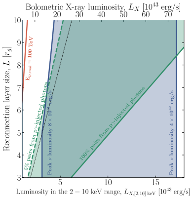
These results allow us to extend the regions in parameter space shown by Fig. 2 to the regime with TeV. We show the corresponding regions in Fig. 4. For large X-ray luminosities, to the right of the thin black dashed line, we enter the fast-cooling regime, where the peak neutrino luminosity scales in proportion to the X-ray luminosity and becomes independent of the size of the reconnection region. This shows that the IceCube neutrino luminosity can also be explained in this fast-cooling regime, and that in fact an even larger amount of pairs can be attained in this regime compared to the marginally-fast cooling.
Appendix C Spherical geometry
The numerical code we use for the radiative calculations (see App. D) is set up for a spherical geometry. Here we discuss the main changes induced by considering a spherical, rather than plane, region. To clearly differentiate between the two cases, we will define as the size of the spherical region. In relating the planar to spherical case, we will choose an effective size for the spherical region by equating the volumes for the sphere and the reconnection region . Therefore, is related to the full-length of the current sheet as .
The energy density of X-rays is now connected to the luminosity by
| (C1) |
From the equality
| (C2) |
we obtain the magnetic energy density
| (C3) | |||
The corresponding magnetic field is
| (C4) |
The acceleration timescale is also changed as
| (C5) |
The escape timescale is left unchanged and is
| (C6) |
For the photohadronic timescale, the change in the X-rays energy density leads to the revised estimate
| (C7) |
Equating this with the escape timescale we find the critical energy
| (C8) |
We similarly find the maximum cooling-limited proton energy as
| (C9) | |||
In the peak neutrino spectrum, we have to account for an additional factor in the denominator coming from the geometrical factors in and in the target photon density, and a correction factor to account for the relative volume factor between the spherical volume and the volume of the layer , leading to the estimate
| (C10) |
Finally, in the estimated number density of pairs, assuming that the fraction of MeV photons can be estimated just as in the planar case, we find
| (C11) |
Notice that in the spherical case, with as discussed above, the pair number density can be much larger compared to the planar case (see Eq. (19)), due to the spherical region being significantly smaller in all directions. Nonetheless, differences found in between the planar and spherical geometry do not affect proton cooling, and in turn our neutrino estimates.
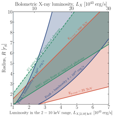
For completeness we show in Fig. 5 the regions of the leading to a pair production comparable with the pair population inferred from Compton opacity, a peak neutrino flux consistent with the IceCube measurements, and TeV. Compared to the planar case of Fig. 2, for a compact enough region () one can simultaneously produce a sizable amount of pairs and saturate the observed neutrino flux, without entering the fast-cooling regime (see also Figs. 3 and 6). This is due to the more compact spherical geometry, which allows for a larger production even at lower luminosities.
Appendix D Numerical approach
We supplement our analytical calculations of the neutrino spectrum with numerical results obtained with the proprietary code athea (Dimitrakoudis et al., 2012). The code solves the kinetic equations for relativistic protons, secondary electrons and positrons, photons, neutrons, and neutrinos. The emitting region is assumed to be spherical with radius . The magnetic field inside the source has strength , and all particle populations inside the source are assumed to be isotropically distributed. The physical processes that are included in athea and couple the various particle species are: electron and proton synchrotron emission, synchrotron self-absorption, electron inverse Compton scattering, pair production, proton-photon (Bethe-Heitler) pair production, proton-photon and neutron-photon pion production. The photomeson interactions are modeled based on the results of the Monte Carlo event generator sophia (Mücke et al., 2000), while Bethe-Heitler production is modeled using the Monte Carlo results of Protheroe & Johnson (1996); see also Mastichiadis et al. (2005). For the modeling of other processes we refer the reader to Mastichiadis & Kirk (1995) and Dimitrakoudis et al. (2012). The code also returns the Thomson optical depth of the source based on the density of electron-positron pairs that cool due to radiative losses down to . We note, however, that these cold pairs are “passive”, because radiative processes of non-relativistic electrons (e.g., cyclotron radiation and Compton scattering) are not included in the numerical code. With the adopted numerical scheme, energy is conserved in a self-consistent way, since all the energy gained by one particle species has to come from an equal amount of energy lost by another particle species. The adopted numerical scheme is ideal for studying the development of in-source electromagnetic cascades in both linear (Zhang et al., 2020) and non-linear regimes where the targets for photohadronic interactions are themselves produced by the proton population (e.g. Petropoulou et al., 2014; Mastichiadis & Petropoulou, 2021).
As discussed in App. C, we consider a spherical region with a radius . All particles escape from the source on an energy-independent timescale . Relativistic protons, after being accelerated into a broken power-law distribution by reconnection (see also Sec. 3.3), are then “injected” into the spherical region at a rate given by
| (D1) |
where , assuming . Here, we introduce to refer to the fraction of energy carried by the proton population in the absence of cooling, as explained in App. B. To compute the steady-state proton distribution and the emerging photon and neutrino emission, we study the system for ; this is also a typical lifetime of the reconnection region, for . Results are shown for , eV, keV, X-ray photon index -2, erg s-1, , , , , , TeV, PeV, G, and cm.
Figure 6 shows the steady-state proton distribution we obtain numerically (thick solid line) and analytically as explained in Sec. 3.3 (cyan markers). The analytical expression describes well the spectral break at , caused by the change in the energy dependence of the photopion loss timescale.
Some key findings from the numerical analysis:
-
•
Protons with energies cool efficiently through photomeson interactions (equivalently, the reconnection region is optically thick to photomeson interactions for protons beyond this energy).
-
•
About 50% of the energy carried initially by the proton population into the radiative zone (i.e., the reconnection downstream) is transferred to secondary particles (resulting in ), with neutrinos taking about 12% of the energy lost by protons.
- •
Appendix E Neutrino emission outside of the reconnection layer
Protons escaping the reconnection layer can provide an additional contribution to the neutrino emission. Photohadronic neutrino production is generally dominated by the reconnection layer, due to the rapid geometric dilution of both the emitted proton population and the X-ray photon field. On the other hand, a reasonable concern is whether proton-proton scattering on the material in the accretion flow can significantly contribute to the neutrino emission. We now show that this is not the case, by estimating the energy-loss timescale due to scattering on the accretion flow gas.
The proton density in the accretion disk can be estimated as
| (E1) |
where denotes the disk’s scale height, and is the radial inflow velocity. Considering that the inner disk is thick, with , due to the disk expansion associated with radiation pressure, and taking and as the azimuthal and the radial velocity, with being the standard parameter from Shakura and Sunyaev theory of accretion disks, we use Eq. A8 and obtain
| (E2) |
where . We can now estimate the energy-loss timescale as (see, e.g., Murase (2018))
| (E3) | |||
where cm2 is the cross section and is the inelasticity. In order to see whether interactions can be fast enough to significantly produce neutrinos, we should compare this timescale with the typical residence time of the protons in the inner region of the accretion disk, after they escape the reconnection layer. If protons are able to freely stream out of the region, such timescale is of the same order of magnitude as the escape timescale from the layer, and therefore the production is negligible. On the other hand, if proton escape is diffusive, their residence time in the disk would be larger, possibly leading to an enhanced production. In any case, since only protons below the cooling energy are able to escape the reconnection layer while still retaining their energy, this additional channel of neutrino production would mostly be relevant at energies near or below the neutrino peak, and therefore would not be observable at IceCube.
A final possibility that one could consider is that neutrons, produced in the reconnection layer by interactions, could escape from it and decay outside, producing neutrinos. However, since the fraction of neutron energy carried by a neutrino in beta decay is typically of the order of (see, e.g., Lipari et al. (2007); Fiorillo et al. (2021)), these neutrinos would appear at much lower energies, in the GeV range. Therefore, we do not account for this contribution in our work.