ZeroNVS: Zero-Shot 360-Degree View
Synthesis from a Single Real Image

Abstract

We introduce a 3D-aware diffusion model, ZeroNVS, for single-image novel view synthesis for in-the-wild scenes. While existing methods are designed for single objects with masked backgrounds, we propose new techniques to address challenges introduced by in-the-wild multi-object scenes with complex backgrounds. Specifically, we train a generative prior on a mixture of data sources that capture object-centric, indoor, and outdoor scenes. To address issues from data mixture such as depth-scale ambiguity, we propose a novel camera conditioning parameterization and normalization scheme. Further, we observe that Score Distillation Sampling (SDS) tends to truncate the distribution of complex backgrounds during distillation of 360-degree scenes, and propose “SDS anchoring” to improve the diversity of synthesized novel views. Our model sets a new state-of-the-art result in LPIPS on the DTU dataset in the zero-shot setting, even outperforming methods specifically trained on DTU. We further adapt the challenging Mip-NeRF 360 dataset as a new benchmark for single-image novel view synthesis, and demonstrate strong performance in this setting. Our code and data are at https://kylesargent.github.io/zeronvs/

1 Introduction

CO3D
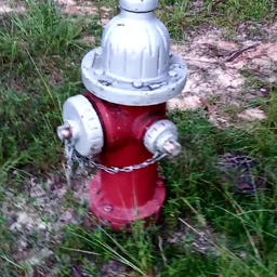
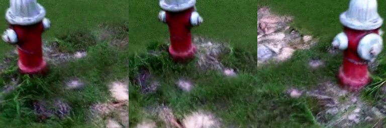
Input view	———————— Novel views ————————	Input view	———————— Novel views ————————
Mip-NeRF 360 (Zero-shot)
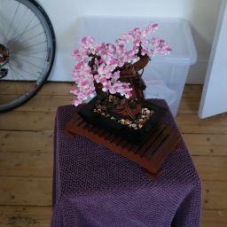
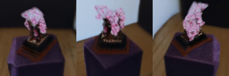
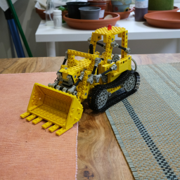
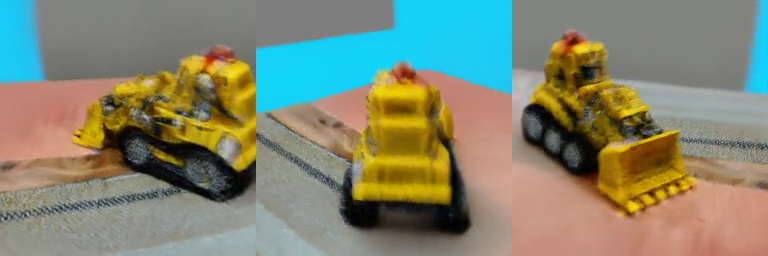
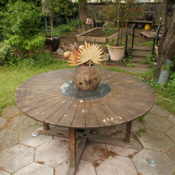
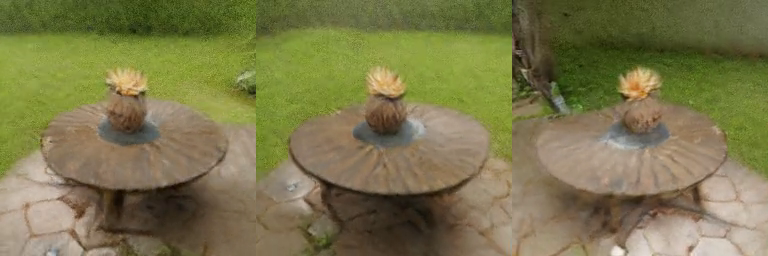
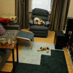
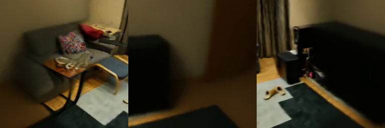
Input view	———————— Novel views ————————	Input view	———————— Novel views ————————
RealEstate10K
Input view	———————— Novel views ————————	Input view	———————— Novel views ————————
DTU (Zero-shot)
Input view	———————— Novel views ————————	Input view	———————— Novel views ————————

Figure 1: Results for view synthesis from a single image. All NeRFs are predicted by the same model.

Models for single-image, 360-degree novel view synthesis (NVS) should produce realistic and diverse results: the synthesized images should look natural and 3D-consistent to humans, and they should also capture the many possible explanations of unobservable regions. This challenging problem has typically been studied in the context of single objects without backgrounds, where the requirements on both realism and diversity are simplified. Recent progresses rely on large datasets of high-quality object meshes like Objaverse-XL (Deitke et al., 2023) which have enabled conditional diffusion models to produce photorealistic images from a novel view, followed by Score Distillation Sampling (SDS; Poole et al., 2022) to improve their 3D consistency. Meanwhile, since image diversity mostly lies in the background, not the object, the ignorance of background significantly lowers the expectation of synthesizing diverse images–in fact, most object-centric methods no longer consider diversity as a metric (Liu et al., 2023b; Melas-Kyriazi et al., 2023; Qian et al., 2023).

Neither assumption holds for the more challenging problem of zero-shot, 360-degree novel view synthesis on real-world scenes. There is no single, large-scale dataset of scenes with ground-truth geometry, texture, and camera parameters, analogous to Objaverse-XL for objects. The background, which cannot be ignored anymore, also needs to be well modeled for synthesizing diverse results.

We address both issues with our new model, ZeroNVS. Inspired by previous object-centric methods (Liu et al., 2023b; Melas-Kyriazi et al., 2023; Qian et al., 2023), ZeroNVS also trains a 2D conditional diffusion model followed by 3D distillation. But unlike them, ZeroNVS works well on scenes due to two technical innovations: a new camera parametrization and normalization scheme for conditioning, which allows training the diffusion model on a collection of diverse scene datasets, and a new “SDS anchoring” mechanism, addressing the limited diversity in scene backgrounds when using standard SDS.

To overcome the key challenge of limited training data, we propose training the diffusion model on a massive mixed dataset comprised of all scenes from CO3D (Reizenstein et al., 2021), RealEstate10K (Zhou et al., 2018), and ACID (Liu et al., 2021), so that the model may potentially handle complex in-the-wild scenes. The mixed data of such scale and diversity are captured with a variety of camera settings and have several different types of 3D ground truth, e.g., computed with COLMAP (Schönberger & Frahm, 2016) or ORB-SLAM (Mur-Artal et al., 2015). We show that while the camera conditioning representations from prior methods (Liu et al., 2023b) are too ambiguous or inexpressive to model in-the-wild scenes, our new camera parametrization and normalization scheme allows exploiting such diverse data sources and leads to superior NVS on real-world scenes.

Building a 2D conditional diffusion model that works effectively for in-the-wild scenes enables us to then study the limitations of SDS in the scene setting. In particular, we observe limited diversity from SDS in the generated scene backgrounds when synthesizing long-range (e.g., 180-degree) novel views. We therefore propose “SDS anchoring” to ameliorate the issue. In SDS anchoring, we propose to first sample several “anchor” novel views using the standard Denoising Diffusion Implicit Model (DDIM) sampling (Song et al., 2021). This yields a collection of pseudo-ground-truth novel views with diverse contents, since DDIM is not prone to mode collapse like SDS. Then, rather than using these views as RGB supervision, we sample from them randomly as conditions for SDS, which enforces diversity while still ensuring 3D-consistent view synthesis.

ZeroNVS achieves strong zero-shot generalization to unseen data. We set a new state-of-the-art LPIPS score on the challenging DTU benchmark, even outperforming methods that were directly fine-tuned on this dataset. Since the popular benchmark DTU consists of scenes captured by a forward-facing camera rig and cannot evaluate more challenging pose changes, we propose to use the Mip-NeRF 360 dataset (Barron et al., 2022) as a single-image novel view synthesis benchmark. ZeroNVS achieves the best LPIPS performance on this benchmark. Finally, we show the potential of SDS anchoring for addressing diversity issues in background generation via a user study.

To summarize, we make the following contributions:

• We propose ZeroNVS, which enables full-scene NVS from real images. ZeroNVS first demonstrates that SDS distillation can be used to lift scenes that are not object-centric and may have complex backgrounds to 3D.

• We show that the formulations on handling cameras and scene scale in prior work are either inexpressive or ambiguous for in-the-wild scenes. We propose a new camera conditioning parameterization and a scene normalization scheme. These enable us to train a single model on a large collection of diverse training data consisting of CO3D, RealEstate10K and ACID, allowing strong zero-shot generalization for NVS on in-the-wild images.

• We study the limitations of SDS distillation as applied to scenes. Similar to prior work, we identify a diversity issue, which manifests in this case as novel view predictions with monotone backgrounds. We propose SDS anchoring to ameliorate the issue.

• We show state-of-the-art LPIPS results on DTU zero-shot, surpassing prior methods finetuned on this dataset. Furthermore, we introduce the Mip-NeRF 360 dataset as a scene-level single-image novel view synthesis benchmark and analyze the performances of our and other methods. Finally, we show that our proposed SDS anchoring is overwhelmingly preferred for diverse generations via a user study.

2 Related work

3D generation. The 3D generative model most relevant to our work is DreamFusion (Poole et al., 2022), which proposed Score Distillation Sampling (SDS) as a way of leveraging a diffusion model to extract a NeRF given a user-provided text prompt. After DreamFusion, follow-up works such as Magic3D (Lin et al., 2023), ATT3D (Lorraine et al., 2023), ProlificDreamer (Wang et al., 2023), and Fantasia3D (Chen et al., 2023) improved the quality, diversity, resolution, or run-time.

Other types of 3D generative models include GAN-based 3D generative models, which are primarily restricted to single object categories (Chan et al., 2021a; Niemeyer & Geiger, 2021; Gu et al., 2022; Chan et al., 2021b; Nguyen-Phuoc et al., 2019; Skorokhodov et al., 2022) or to synthetic data (Gao et al., 2022). Recently, 3DGP (Skorokhodov et al., 2023) adapted the GAN-based approach to train 3D generative models on ImageNet. VQ3D (Sargent et al., 2023) and IVID (Xiang et al., 2023) leveraged vector quantization and diffusion, respectively, to learn 3D-aware generative models on ImageNet. Different from the diffusion work outlined above, IVID used mesh-based warping and diffusion inpainting rather than distillation to achieve high-quality synthesis results.

Single-image novel view synthesis. Prior to diffusion models, works typically focused on learning image-based feature extractors which could be trained end-to-end with some level of 3D supervision. PixelNeRF (Yu et al., 2021) learns a prior over 3D scenes via training a CNN-based feature extractor and differentiable un-projection of a feature frustum inferred from one or more input images. Similarly, DietNeRF (Jain et al., 2021) can infer NeRFs from one or few images via a training strategy geared towards semantic consistency. Different from these works, ZeroNVS infers novel views which resemble crisp natural images, and furthermore is capable of extensive camera viewpoint change, i.e., up to 360 degrees of camera motion.

Several diffusion-based approaches have recently emerged for novel view synthesis of objects. One prominent paradigm separates novel view synthesis into two stages; first, a (potentially 3D-aware) diffusion model is trained, and second, the diffusion model is used to distill 3D-consistent scene representations given an input image via techniques like score distillation sampling (Poole et al., 2022), score Jacobian chaining (Wang et al., 2022), textual inversion or semantic guidance leveraging the diffusion model (Melas-Kyriazi et al., 2023; Deng et al., 2022a), or explicit 3D reconstruction from multiple sampled views of the diffusion model (Liu et al., 2023a; c). Unlike these works, ZeroNVS is trained on large real scene datasets and performs scene-level novel view synthesis.

Other works more explicitly embed a 3D-aware inductive bias into a unified diffusion model architecture; for example, HoloDiffusion (Karnewar et al., 2023) trains a 3D diffusion model to generate 3D objects. Concurrent works include GenVS (Chan et al., 2023), Forward Models (Tewari et al., 2023), and IVID (Xiang et al., 2023). While GenVS and Forward Models train and evaluate models on one scene category, such as fire hydrants or rooms, at a time, ZeroNVS handles both such scene categories and more in a single model.

Depth estimation. Though ZeroNVS estimates depth as part of 3D SDS distillation, depth estimation is not the emphasis of our work. However, our work draws significant philosophical inspiration from the landmark paper MIDAS (Ranftl et al., 2022). MIDAS demonstrated that selecting a training objective (scale- and shift-invariant inverse depth estimation) which is compatible with many different data sources can significantly increase the amount of training data that can be leveraged. Then, even though the model predicts inverse depth maps without a known scale or shift, the strong zero-shot performance from leveraging massive datasets means the model is widely used in practice after finetuning (Bhat et al., 2023) or manually choosing reasonable scale and shift estimates (Jampani et al., 2021). Thus, our technical innovations in camera conditioning representation and scene normalization are motivated by the value demonstrated in MIDAS of being able to leverage multiple diverse data sources.

3 Approach

We consider the problem of scene-level novel view synthesis from a single real image. Similar to prior work (Liu et al., 2023b; Qian et al., 2023), we first train a diffusion model $\mathbf{p}_{\theta}$ to perform novel view synthesis, and then leverage it to perform 3D SDS distillation. Unlike prior work, we focus on scenes rather than objects. Scenes present several unique challenges. First, prior works use representations for cameras and scale which are either ambiguous or insufficiently expressive for scenes. Second, the inference procedure of prior works is based on SDS, which has a known mode collapse issue and which manifests in scenes through greatly reduced background diversity in predicted views. We will attempt to address these challenges through improved representations and inference procedures for scenes compared with prior work (Liu et al., 2023b; Qian et al., 2023).

We shall begin the discussion of our approach by introducing some general notation. Let a scene $S$ be comprised of a set of images $X=\{X_{i}\}_{i=1}^{n}$, depth maps $D=\{D_{i}\}_{i=1}^{n}$, extrinsics $E=\{E_{i}\}_{i=1}^{n}$, and a shared field-of-view $f$. We note that an extrinsics matrix $E_{i}$ can be identified with its rotation and translation components, defined by $E_{i}=(E_{i}^{R},E_{i}^{T})$. We preprocess the datasets to consist of square images and assume intrinsics are shared within a given scene, and that there is no skew, distortion, or off-center principal point.

We will focus on the design of the conditional information which is passed to the view synthesis diffusion model $\mathbf{p}_{\theta}$ in addition to the input image. This conditional information can be represented via a function, $\mathbf{M}(D,f,E,i,j)$, which computes a conditioning embedding given the full sets of depths and extrinsics for the scene, the field of view, and the indices $i,j$ of the input and target view respectively. We learn a generative model over novel views following a parameterized distribution $\mathbf{p_{\theta}}$, so that we have

$$X_{j}\sim\mathbf{p_{\theta}}(X_{j}|X_{i},\mathbf{M}(D,f,E,i,j))~{}.$$

The output of $\mathbf{M}$ and the (single) input image $X_{i}$ are the only information available to the model for view synthesis.

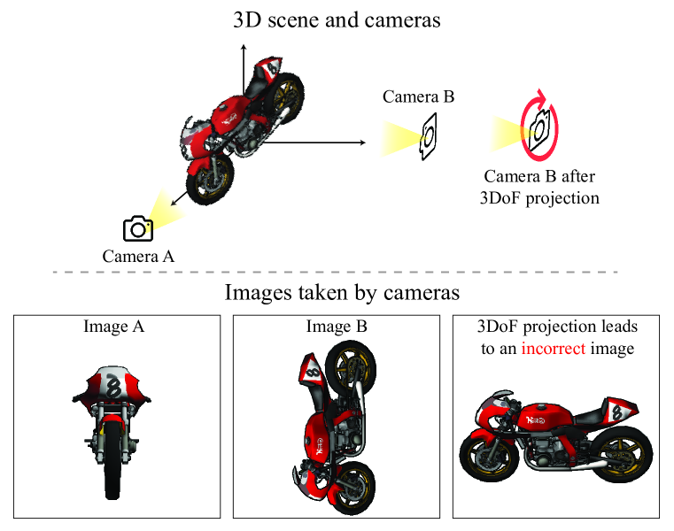
Figure 2: A 3DoF camera pose captures camera elevation, azimuth, and radius for a camera pointed at the origin but is incapable of representing a camera’s roll (pictured) or cameras oriented arbitrarily in space. A model with this parameterization cannot be trained on real-world data, where many of the camera poses are inadequately represented by a 3DoF pose.

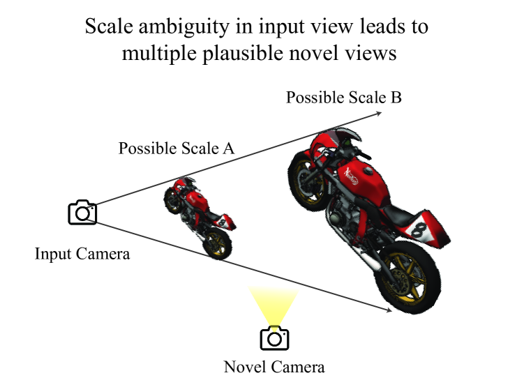
Figure 3: To a monocular camera, a small object close to the camera (left) and a large object at a distance (right) appear identical, despite representing different scenes. Scale ambiguity in the input view causes ambiguity in novel view synthesis. Specifically, even after conditioning on the image taken from the input view, an image taken from the novel camera could either have a small motorcycle on the left (Scale A) or a large motorcycle on the right (Scale B).

Both Zero-1-to-3 (Section 3.1) and our model, as well as several intermediate models that we will study (Sections 3.2 and 3.3), can be regarded as different choices for $\mathbf{M}$. As we illustrate in Figures 3, 3, 5 and 5, and verify later in experiments, different choices for $\mathbf{M}$ can have drastic impacts on the model’s performance.

At inference time, information such as the full set of depth maps $D$ or extrinsics $E$ for a scene may not be known. But, analogous to MIDAS where the scale and shift for predictions may be unknown, we see that in practice, an approximate guess for the evaluation of $\mathbf{M}$ suffices.

3.1 Representing objects for view synthesis

Zero-1-to-3 (Liu et al., 2023b) represents poses with 3 degrees of freedom, given by an elevation angle $\theta$, azimuth angle $\phi$, and radius $z$. Let $\mathbf{P}:\mathrm{SE}(3)\rightarrow\mathbb{R}^{3}$ be the projection to this representation, then

$$\mathbf{M}_{\mathrm{Zero-1-to-3}}(D,f,E,i,j)=\mathbf{P}(E_{i})-\mathbf{P}(E_{j})$$

is the camera conditioning representation used by Zero-1-to-3. For object mesh datasets such as Objaverse (Deitke et al., 2022) and Objaverse-XL (Deitke et al., 2023), this representation is appropriate because the data is known to consist of single objects without backgrounds, aligned and centered at the origin and imaged from training cameras generated with three degrees of freedom. However, such a parameterization limits the model’s ability to generalize to non-object-centric images. Zero-1-to-3 proposed mitigating the distribution mismatch by applying a foreground segmentation model and then centering the content (Qian et al., 2023; Liu et al., 2023a).

While this 3DoF camera parameterization is an effective solution for object-centered and aligned images, it is insufficient for representing cameras for real-world data, where each pose can have six degrees of freedom, incorporating both rotation (pitch, roll, yaw) and 3D translation. An illustration of a failure of the 3DoF camera representation due to the camera’s roll is shown in Figure 3. Moreover, the use of synthetic object datasets limits the applicability of the model to scenes with a foreground object that can be extracted via a segmentation model.

3.2 Representing generic scenes for view synthesis

For scenes, we should use a camera representation with six degrees of freedom that can capture all possible positions and orientations. One straightforward choice for a camera parameterization that captures six degrees of freedom is the relative pose parameterization (Watson et al., 2023). We propose to also include the field of view as an additional degree of freedom. We term this combined representation “6DoF+1”. This gives us

$$\mathbf{M}_{\mathrm{6DoF+1}}(D,f,E,i,j)=[E_{i}^{-1}E_{j},f].$$

One attractive property of $\mathbf{M}_{\mathrm{6DoF+1}}$ is that it is invariant with respect to a rigid transformation $\tilde{E}$ of the scene, so that we have

$$\mathbf{M}_{\mathrm{6DoF+1}}(D,f,\tilde{E}\cdot E,i,j)=[(\tilde{E}\cdot E_{i})^{-1}\tilde{E}\cdot E_{j},f]=[E_{i}^{-1}E_{j},f]~{},$$

implying $\mathbf{M}_{\mathrm{6DoF+1}}$ is invariant to translating the scene center and/or rotating the scene. This is useful given the arbitrary nature of the poses for our datasets, namely CO3D, ACID, and RealEstate10K, which are determined by COLMAP or ORB-SLAM. The poses discovered via these algorithms are not related to any semantically meaningful alignment of the scene’s content, such as a rigid transformation and scale transformation, which align the scene to some canonical frame and unit of scale.

Although we have seen that $\mathbf{M}_{\mathrm{6DoF+1}}$ is invariant to rigid transformations of the scene, it is not invariant to scale. The scene scales determined by COLMAP and ORB-SLAM are also arbitrary, and in practice may vary by orders of magnitude. One solution is to simply normalize the camera locations to have, on average, the unit norm when the mean of the camera locations is chosen as the origin. Let $\mathbf{R}(E,\lambda):\textrm{SE}(3)\times\mathbb{R}\rightarrow\textrm{SE}(3)$ be a function that scales the translation component of the extrinsic matrix $E$ by $\lambda$. Then we define

$$s =\frac{1}{n}\sum\limits_{i=1}^{n}\|E_{i}^{T}-\frac{1}{n}\sum\limits_{j=1}^{n}E_{j}^{T}\|_{2}~{},$$

$$\mathbf{M}_{\mathrm{6DoF+1,~{}norm.}}(D,f,E,i,j) =\Big{[}\mathbf{R}\Big{(}E_{i},\frac{1}{s}\Big{)}^{-1}\mathbf{R}\Big{(}E_{j},\frac{1}{s}\Big{)},f)\Big{]}~{},$$

where $s$ is the average norm of the camera locations when the mean of the camera locations is chosen as the origin. In $\mathbf{M}_{\mathrm{6DoF+1,~{}norm.}}$, the camera locations are normalized via rescaling by $\frac{1}{s}$, in contrast to $\mathbf{M}_{\mathrm{6DoF+1}}$ where the scales are arbitrary. This choice of $\mathbf{M}$ assures that scenes from our mixture of datasets will have similar scales.

3.3 Addressing scale ambiguity with a new normalization scheme

The representation $\mathbf{M}_{\mathrm{6DoF+1,~{}norm.}}$ achieves reasonable performance on real scenes by addressing issues in prior representations with limited degrees of freedom and handling of scale. However, performance can be further improved. In this section, we show that a more effective normalization scheme that better addresses scale ambiguity leads to improved performance.

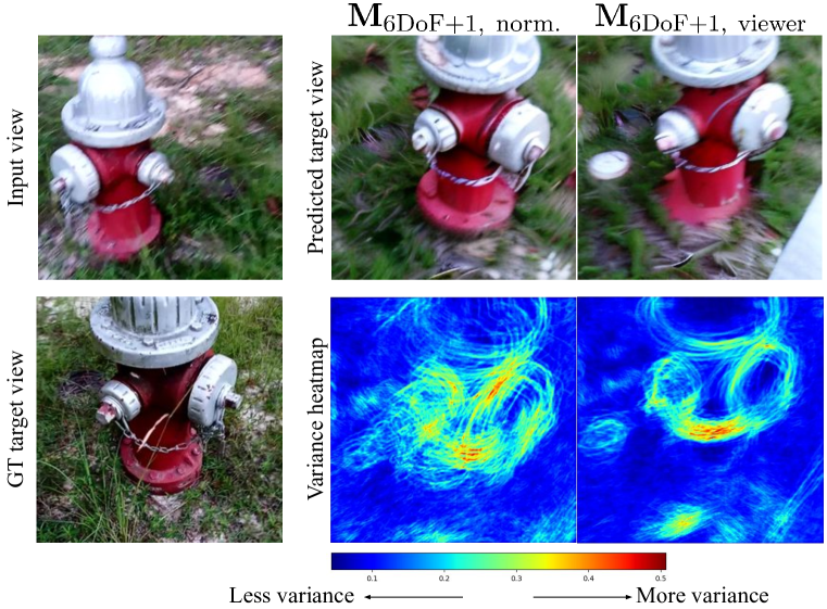
Figure 4: For each normalization scheme, we show heatmaps of the variance of the Sobel edge maps of multiple samples from ZeroNVS. Our proposed scheme $\mathbf{M}_{\mathrm{6DoF+1,~{}viewer}}$ reduces randomness due to scale ambiguity.

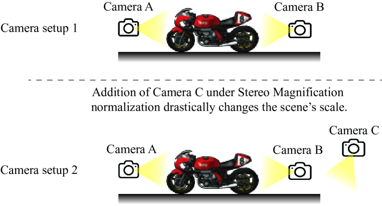
Figure 5: Top: A scene with two cameras facing the object. Bottom: The same scene with a new camera added facing the ground. Aggregating the cameras before computing the scale would lead to different computed scales for each setup. Our proposed viewer-centric normalization avoids this and reduces scale ambiguity.

The scene scale is ambiguous given a monocular input image. This ambiguity has been discussed extensively in the context of monocular estimation (Ranftl et al., 2022; Yin et al., 2022), but is also present in novel view synthesis, as demonstrated by Figure 3. Sampling a novel view via conditioning with a representation like $\mathbf{M}_{\mathrm{6DoF+1,~{}norm.}}$ that contains no information about the scale of visible content in the input image amounts to sampling an image from the distribution of images marginalizing over the unknown scale. This leads to more uncertain novel view synthesis, as can be seen in Figure 5), and additionally to poorer 3D distillation performance, as we show later in experiments.

We instead choose to condition on the scale by introducing information about the scale of the visible content to our conditioning embedding function $\mathbf{M}$. Rather than normalize by camera locations, Stereo Magnification (Zhou et al., 2018) takes the 5-th quantile of each depth map of the scene, and then takes the 10-th quantile of this aggregated set of numbers, and declares this as the scene scale. Let $\mathbf{Q}_{k}$ be a function which takes the $k$-th quantile of a set of numbers, then we define

$$q =\mathbf{Q}_{10}(\{\mathbf{Q}_{5}(D_{i})\}_{i=1}^{n})~{},$$

$$\mathbf{M}_{\mathrm{6DoF+1,~{}agg.}}(D,f,E,i,j) =\Big{[}\mathbf{R}\Big{(}E_{i},\frac{1}{q}\Big{)}^{-1}\mathbf{R}\Big{(}E_{j},\frac{1}{q}\Big{)},f\Big{]}~{},$$

where in $\mathbf{M}_{\mathrm{6DoF+1,~{}agg.}}$, $q$ is the scale applied to the translation component of the scene’s cameras before computing the relative pose. In this way $\mathbf{M}_{\mathrm{6DoF+1,~{}agg.}}$ is different from $\mathbf{M}_{\mathrm{6DoF+1,~{}norm.}}$ because the camera conditioning representation contains information about the scale of the visible content from the depth maps $D_{i}$ in addition to the change in orientation between the input and target view. Although conditioning on the scale in this way improves performance, there are two issues with $\mathbf{M}_{\mathrm{6DoF+1,~{}agg.}}$. The first arises from aggregating the quantiles over all the images. In Figure 5, adding an additional Camera C to the scene changes the value of $\mathbf{M}_{\mathrm{6DoF+1,~{}agg.}}$ despite nothing else having changed about the scene. This makes the view synthesis task from either Camera A or Camera B more ambiguous. To ensure this is impossible, we can simply eliminate the aggregation step over the quantiles of all depth maps in the scene.

The second issue arises from different depth statistics within the mixture of datasets we use for training. Both COLMAP and ORB-SLAM infer sparse point clouds for scenes which are then rendered at the inferred poses to produce the sparse depth maps $D_{i}$. However, ORB-SLAM generally produces sparser depth maps than COLMAP, and therefore the value of $\mathbf{Q}_{k}$ may have different meanings for each dataset. We therefore use an off-the-shelf depth estimator (Ranftl et al., 2021) to fill holes in the depth maps. We denote the depth $D_{i}$ infilled in this way as $\bar{D}_{i}$. We then apply $\mathbf{Q}_{k}$ to dense depth maps $\bar{D}_{i}$ instead. We emphasize that the depth estimator is not used during inference or distillation. Its purpose is only for the model to learn a consistent definition of scale during training, which it may then apply to generate low-variance predictions (see Figure 5).

These two fixes lead to our proposed normalization, which is fully viewer-centric. We define it as

$$q_{i} =\mathbf{Q}_{20}(\bar{D}_{i})~{},$$

$$\mathbf{M}_{\mathrm{6DoF+1,~{}viewer}}(D,f,E,i,j) =\Big{[}\mathbf{R}\Big{(}E_{i},\frac{1}{q_{i}}\Big{)}^{-1}\mathbf{R}\Big{(}E_{j},\frac{1}{q_{i}}\Big{)},f\Big{]}~{},$$

where in $\mathbf{M}_{\mathrm{6DoF+1,~{}viewer}}$, the scale $q_{i}$ applied to the cameras is dependent only on the depth map in the input view $\bar{D}_{i}$, different from $\mathbf{M}_{\mathrm{6DoF+1,~{}agg.}}$ where the scale $q$ computed by aggregating over all $D_{i}$. At inference, analogous to scale and shift for MIDAS, the value of $q_{i}$ can be chosen heuristically without compromising performance. Correcting for the scale ambiguities in this way eliminates one source of randomness for view synthesis. This leads to improved metrics, which we show in Section 4.

3.4 Improving diversity with SDS anchoring

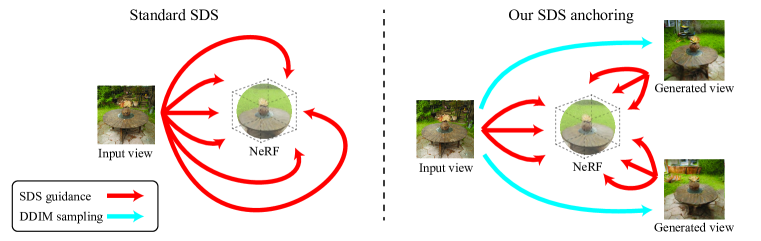
Figure 6: SDS-based NeRF distillation (left) uses the same guidance image for all 360 degrees of novel views. Our “SDS anchoring” (right) first samples novel views via DDIM (Song et al., 2020), and then uses the nearest image (whether the input or a sampled novel view) for guidance.

Diffusion models trained with the improved camera conditioning representation $\mathbf{M}_{\mathrm{6DoF+1,~{}viewer}}$ achieve superior view synthesis results via 3D SDS distillation. However, for large viewpoint changes, novel view synthesis is also a generation problem, and it may be desirable to generate diverse and plausible contents rather than contents that are only optimal on average for metrics such as PSNR, SSIM, and LPIPS. However, Poole et al. (2022) noted that even when the underlying generative model produces diverse images, SDS distillation of that model tends to seek a single mode. For novel view synthesis of scenes via SDS, we observe a unique manifestation of this diversity issue: lack of diversity is especially apparent in inferred backgrounds. Often, SDS distillation predicts a gray or monotone background for regions not observed by the input camera.

To remedy this, we propose “SDS anchoring” (Figure 6). Typically, when using a view-conditioned diffusion model for novel view synthesis, we optimize an SDS objective for renderings $\tilde{X}$ with the diffusion model $\epsilon_{\theta}$ conditioned on the input view $X_{i}$. We have

$$\mathcal{L}_{\text{SDS}}(\tilde{X})=\|w(\sigma)(\epsilon_{\theta}(\tilde{X}+\epsilon,X_{i},\mathbf{M}(D,f,E,i,j))-\epsilon)\|^{2}_{2},$$

where $\sigma\sim\mathcal{U}(\sigma_{\text{min}},\sigma_{\text{max}})$, and $\epsilon\sim\mathcal{N}(0,\sigma^{2}\mathbf{I})$. With SDS anchoring, we first directly sample, via iterative denoising, $k$ novel views $\bm{\hat{X}}_{k}=\{\hat{X}_{j}\}_{j=1}^{k}$ with $\hat{X}_{j}\sim p(X_{j}|X_{i},\mathbf{M}(D,f,E,i,j))$ from poses evenly spaced in azimuth for maximum scene coverage. Each novel view is generated conditional on the input view. Then, when optimizing the SDS objective, we condition the diffusion model not on the input view, but on the nearest view in the geodesic distance on $SO(3)$ from $\bm{\hat{X}}_{k}\cup\{X_{i}\}$, which we define as $X_{i_{\text{nearest}}}$. Then we have

$$\mathcal{L}_{\text{SDS anchoring}}(\tilde{X})=\|w(\sigma)(\epsilon_{\theta}(\tilde{X}+\epsilon,X_{i_{\text{nearest}}},\mathbf{M}(D,f,E,i,j))-\epsilon)\|^{2}_{2}.$$

Although SDS anchoring might in principle produce 3D-inconsistent scenes, we see that in practice it tends to smooth out inconsistencies. As shown in Section 4, SDS anchoring produces more diverse background contents. We provide more details about the setup of SDS anchoring in Appendix B.

4 Experiments

We first describe the setup of our model and experiments. Then we cover our main experimental results on zero-shot 3D consistent novel view synthesis. We conduct extensive ablations and finally provide qualitative analysis of our contributions and design choices.

4.1 Setup

Datasets. Our models are trained on a mixture dataset consisting of CO3D (Reizenstein et al., 2021), ACID (Liu et al., 2021), and RealEstate10K (Zhou et al., 2018). Each example is sampled uniformly at random from the three datasets. We train at $256\times 256$ resolution, center-cropping and adjusting the intrinsics for each image and scene as necessary. We train with our camera conditioning representation $\mathbf{M}_{\mathrm{6DoF+1,~{}viewer}}$ unless otherwise specified, i.e., as in ablation. To train on this large dataset, we implement a high-performance dataloader using WebDataset (Breuel, 2020). We provide more training details in Appendix A.

We evaluate our trained diffusion models on held-out subsets of CO3D, ACID, and RealEstate10K respectively, for 2D novel view synthesis. Our main evaluations are for zero-shot 3D consistent novel view synthesis, where we compare against other techniques on the DTU benchmark (Aanæs et al., 2016) and on the Mip-NeRF 360 dataset (Barron et al., 2022). We evaluate all models at $256\times 256$ resolution except for DTU, for which we use $400\times 300$ resolution to be comparable to prior art.

Implementation details. Our diffusion model training code is written in PyTorch and based on the public code for Zero-1-to-3 (Liu et al., 2023b). We initialize from the pretrained Zero-1-to-3-XL, swapping out the conditioning module to accommodate our novel parameterizations. Our distillation code is implemented in Threestudio (Guo et al., 2023). We use a custom NeRF network combining various features of Mip-NeRF 360 with Instant-NGP (Müller et al., 2022). The noise schedule is annealed following Wang et al. (2023). For details, please consult Appendix B.

4.2 Main results

Input view	GT novel view	ZeroNVS (ours)	PixelNeRF
		PSNR=10.8, SSIM=0.22	PSNR=12.2, SSIM=0.30

Figure 7: Limitations of PSNR and SSIM for view synthesis evaluation. Misalignments can lead to worse PSNR and SSIM values for predictions that are more semantically sensible.

GT novel view	Zero-1-to-3	NerDi	ZeroNVS (ours)

Figure 8: Qualitative comparison between baseline methods and our method.

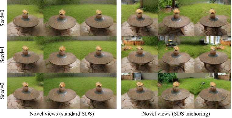
Figure 9: Qualitative depiction of the effects of SDS anchoring. Whereas standard SDS (left) tends to predict monotonous backgrounds, our SDS anchoring (right) generates more diverse background contents. Additionally, SDS anchoring generates different results depending on the random seed, while standard SDS is prone to mode collapse.

NVS on DTU	LPIPS $\downarrow$	PSNR $\uparrow$	SSIM $\uparrow$
$\textrm{DS-NeRF}^{\dagger}$	0.649	12.17	0.410
PixelNeRF	0.535	15.55	0.537
SinNeRF	0.525	16.52	0.560
DietNeRF	0.487	14.24	0.481
NeRDi	0.421	14.47	0.465
ZeroNVS (ours)	0.380	13.55	0.469

Table 1: SOTA comparison. We set a new state-of-the-art for LPIPS on DTU despite being the only method not fine-tuned on DTU. $\dagger=$ Performance reported in Xu et al. (2022).

NVS	LPIPS $\downarrow$	PSNR $\uparrow$	SSIM $\uparrow$
Mip-NeRF 360 Dataset
Zero-1-to-3	0.667	11.7	0.196
PixelNeRF	0.718	16.5	0.556
ZeroNVS (ours)	0.625	13.2	0.240
DTU Dataset
Zero-1-to-3	0.472	10.70	0.383
PixelNeRF	0.738	10.46	0.397
ZeroNVS (ours)	0.380	13.55	0.469

Table 2: Zero-shot comparison. Comparison with baselines trained on our mixture dataset.

We evaluate all methods using the standard set of novel view synthesis metrics: PSNR, SSIM, and LPIPS. We weigh LPIPS more heavily in the comparison due to the well-known issues with PSNR and SSIM as discussed in (Deng et al., 2022a; Chan et al., 2023). We confirm that PSNR and SSIM do not correlate well with performance in our problem setting, as illustrated in Figure 7.

The results are shown in Table 2. We first compare against baseline methods DS-NeRF (Deng et al., 2022b), PixelNeRF (Yu et al., 2021), SinNeRF (Xu et al., 2022), DietNeRF (Jain et al., 2021), and NeRDi (Deng et al., 2022a) on DTU. Although all these methods are trained on DTU, we achieve a state-of-the-art LPIPS zero-shot, having never trained on DTU. We show some qualitative comparisons in Figure 8.

DTU scenes are limited to relatively simple forward-facing scenes. Therefore, we introduce a more challenging benchmark dataset, the Mip-NeRF 360 dataset, to benchmark the task of 360-degree view synthesis from a single image. We use this benchmark as a zero-shot benchmark, and train three baseline models on our mixture dataset to compare zero-shot performance. Restricting to these zero-shot models, our method is the best on LPIPS for this dataset by a wide margin. On DTU, we exceed Zero-1-to-3 and the zero-shot PixelNeRF model on all metrics, not just LPIPS. Performance is shown in Table 2. All numbers for our method and Zero-1-to-3 are for NeRFs predicted from SDS distillation unless otherwise noted.

Limited diversity is a known issue with SDS-based methods, but the long run time makes typical generation-based metrics such as FID cost-prohibitive. Therefore, we quantify the improved diversity from using SDS anchoring via a user study on the Mip-NeRF 360 dataset. A total of 21 users were asked to rate each inferred scene from both ZeroNVS and ZeroNVS with anchoring, based on the scene’s realism, creativity, and their overall preference. The results, shown in Table 4, show a strong human preference for the more diverse scenes generated via SDS anchoring. In addition, Figure 9 includes qualitative examples that show the advantages of SDS anchoring.

User study	% that prefer SDS anchoring
Realism	78%
Creativity	82%
Overall	80%

Table 3: The effectiveness of SDS anchoring. Users prefer scenes distilled with SDS anchoring, especially in terms of creativity.

NVS on DTU	LPIPS $\downarrow$	PSNR $\uparrow$	SSIM $\uparrow$
All datasets	0.421	12.2	0.444
-ACID	0.446	11.5	0.405
-CO3D	0.456	10.7	0.407
-RealEstate10K	0.435	12.0	0.429

Table 4: Ablation study on training data. Training on all datasets improves performance.

4.3 Ablation studies

We verify the benefits of using multiple multiview scene datasets in Table 4. Removing either CO3D, ACID, or RealEstate10K results in a model that performs worse than using all three, even for the DTU dataset, where ACID or RealEstate10K might be expected to be mostly out-of-distribution. This confirms the importance of diverse data.

In Table 5, we analyze the diffusion model’s performance on the held-out subsets of our datasets, with the various parameterizations discussed in Section 3. We see that as the conditioning parameterization is further refined, the performance continues to increase. Due to computational constraints, we train the ablation diffusion models for fewer steps than our main model, hence the slightly worse performance relative to Table 2.

	2D novel view synthesis									3D NeRF distillation
	CO3D			RealEstate10K			ACID			DTU
Conditioning	PSNR	SSIM	LPIPS	PSNR	SSIM	LPIPS	PSNR	SSIM	LPIPS	PSNR	SSIM	LPIPS
$\mathbf{M}_{\mathrm{Zero-1-to-3}}$	12.0	.366	.590	11.7	.338	.534	15.5	.371	.431	10.3	.384	.477
$\mathbf{M}_{\mathrm{6DoF+1}}$	12.2	.370	.575	12.5	.380	.483	15.2	.363	.445	9.5	.347	.472
$\mathbf{M}_{\mathrm{6DoF+1,~{}norm.}}$	12.9	.392	.542	12.9	.408	.450	16.5	.398	.398	11.5	.422	.421
$\mathbf{M}_{\mathrm{6DoF+1,~{}agg.}}$	13.2	.402	.527	13.5	.441	.417	16.9	.411	.378	12.2	.436	.420
$\mathbf{M}_{\mathrm{6DoF+1,~{}viewer}}$	13.4	.407	.515	13.5	.440	.414	17.1	.415	.368	12.2	.444	.421

Table 5: Ablation study on the conditioning representation $\mathbf{M}$. Our conditioning representation ($\mathbf{M}_{\mathrm{6DoF+1,~{}viewer}}$) matches or outperforms other conditioning representations.

We provide more details on experimental setups in Appendix C.

5 Conclusion

We have introduced ZeroNVS, a system for 3D-consistent novel view synthesis from a single image for generic scenes. We showed its state-of-the-art performance on existing scene-level novel view synthesis benchmarks and introduced a new and more challenging benchmark, the Mip-NeRF 360 dataset. ZeroNVS can be easily integrated into the pipelines of existing works that leverage 3D-aware diffusion models for downstream applications.

Appendix A Details: Diffusion model training

A.1 Model

We train diffusion models for various camera conditioning parameterizations: $\mathbf{M}_{\mathrm{Zero-1-to-3}}$, $\mathbf{M}_{\mathrm{6DoF+1}}$, $\mathbf{M}_{\mathrm{6DoF+1,~{}norm.}}$, $\mathbf{M}_{\mathrm{6DoF+1,~{}agg.}}$, and $\mathbf{M}_{\mathrm{6DoF+1,~{}viewer}}$. Our runtime is identical to Zero-1-to-3 (Liu et al., 2023b) as the camera conditioning novelties we introduce add negligible overhead and can be done mainly in the dataloader. We train our main model for $60,000$ steps with batch size $1536$. We find that performance tends to saturate after about $20,000$ steps for all models, though it does not decrease. For inference of the 2D diffusion model, we use $500$ DDIM steps and guidance scale $3.0$.

Details for

$\mathbf{M}_{\mathrm{6DoF+1}}$: To embed the field of view $f$ in radians, we use a $3$-dimensional vector consisting of $[f,\sin(f),\cos(f)].$ When concatenated with the $4\times 4=16$-dimensional relative pose matrix, this gives a $19$-dimensional conditioning vector.

Details for

$\mathbf{M}_{\mathrm{6DoF+1,~{}viewer}}$: We use the DPT-SwinV2-256 depth model (Ranftl et al., 2021) to infill depth maps from ORB-SLAM and COLMAP on the ACID, RealEstate10K, and CO3D datasets. We infill the invalid depth map regions only after aligning the disparity from the monodepth estimator to the ground-truth sparse depth map via the optimal scale and shift following Ranftl et al. (2022). We downsample the depth map $4\times$ so that the quantile function is evaluated quickly.

At inference time, the value of $\mathbf{Q}_{20}(\bar{D})$ may not be known since input depth map $D$ is unknown. Therefore there is a question of how to compute the conditioning embedding at inference time. Values of $\mathbf{Q}_{20}(\bar{D})$ between $.7-1$. work for most images and it can be chosen heuristically. For instance, for DTU we uniformly assume a value of $.7$, which seems to work well. Note that any value of $\mathbf{Q}_{20}(\bar{D})$ is presumably possible; it is only when this value is incompatible with the desired SDS camera radius that distillation may fail, since the cameras may intersect the visible content.

A.2 Dataloader

One significant engineering component of our work is our design of a streaming dataloader for multiview data, built on top of WebDataset (Breuel, 2020). Each dataset is sharded and each shard consists of a sequential tar archive of scenes. The shards can be streamed in parallel via multiprocessing. As a shard is streamed, we yield random pairs of views from scenes according to a “rate” parameter that determines how densely to sample each scene. This parameter allows a trade-off between fully random sampling (lower rate) and biased sampling (higher rate) which can be tuned according to the available network bandwidth. Individual streams from each dataset are then combined and sampled randomly to yield the mixture dataset. We will release the code together with our main code release.

Appendix B Details: NeRF prediction and distillation

B.1 SDS Anchoring

We propose SDS anchoring in order to increase the diversity of synthesized scenes. We sample 2 anchors at 120 and 240 degrees of azimuth relative to the input camera.

One potential issue with SDS anchoring is that if the samples are 3D-inconsistent, the resulting generations may look unusual. Furthermore, traditional SDS already performs quite well except if the criterion is diverse backgrounds. Therefore, to implement anchoring, we randomly choose with probability $.5$ either the input camera and view or the nearest sampled anchor camera and view as guidance. If the guidance is an anchor, we ”gate” the gradients flowing back from SDS according to the depth of the NeRF render, so that only depths above a certain threshold ($1.0$ in our experiments) receive guidance from the anchors. This seems to mostly mitigate artifacts from 3D-inconsistency of foreground content, while still allowing for rich backgrounds. We show video results for SDS anchoring on the webpage.

B.2 Hyperparameters

NeRF distillation via involves numerous hyperparameters such as for controlling lighting, shading, camera sampling, number of training steps, training at progressively increasing resolutions, loss weights, density blob initializations, optimizers, guidance weight, and more. We will share a few insights about choosing hyperparameters for scenes here, and release the full configs as part of our code release.

Noise scheduling:

We found that ending training with very low maximum noise levels such as $.025$ seemed to benefit results, particularly perceptual metrics like LPIPS. We additionaly found a significant benefit on 360-degree scenes such as in the Mip-NeRF 360 dataset to scheduling the noise ”anisotropically;” that is, reducing the noise level more slowly on the opposite end from the input view. This seems to give the optimization more time to solve the challenging 180-degree views at higher noise levels before refining the predictions at low noise levels.

Miscellaneous:

Progressive azimuth and elevation sampling following (Qian et al., 2023) was also found to be very important for training stability. Training resolution progresses stagewise, first with batch size 6 at 128x128 and then with batch size $1$ at $256\times 256$.

Appendix C Experimental setups

For our main results on DTU and Mip-NeRF 360, we train our model and Zero-1-to-3 for $60,000$ steps. Performance for our method seems to saturate earlier than for Zero-1-to-3, which trained for about $100,000$ steps; this may be due to the larger dataset size. Objaverse, with $800,000$ scenes, is much larger than the combination of RealEstate10K, ACID, and CO3D, which are only about $95,000$ scenes in total.

For the retrained PixelNeRF baseline, we retrained it on our mixture dataset of CO3D, ACID, and RealEstate10K for about $560,000$ steps.

C.1 Main results

For all single-image NeRF distillation results, we assume the camera elevation, field of view, and content scale are given. These parameters are identical for all DTU scenes but vary across the Mip-NeRF 360 dataset. For DTU, we use the standard input views and test split from from prior work. We select Mip-NeRF 360 input view indices manually based on two criteria. First, the views are well-approximated by a 3DoF pose representation in the sense of geodesic distance between rotations. This is to ensure fair comparison with Zero-1-to-3, and for compatibility with Threestudio’s SDS sampling scheme, which also uses 3 degrees of freedom. Second, as much of the scene content as possible must be visible in the view. The exact values of the input view indices are given in Table 6.

The field of view is obtained via COLMAP. The camera elevation is set automatically via computing the angle between the forward axis of the camera and the world’s $XY$-plane, after the cameras have been standardized via PCA following Barron et al. (2022).

One challenge is that for both the Mip-NeRF 360 and DTU datasets, the scene scales are not known by the zero-shot methods, namely Zero-1-to-3, our method, and our retrained PixelNeRF. Therefore, for the zero-shot methods, we manually grid search for the optimal world scale in intervals of $.1$ to find the appropriate world scale for each scene in order to align the predictions to the generated scenes. Between five to nine samples within $[.3,.4,.5,.6,.7,.8,.9,1.,1.1,1.2,1.3,1.4,1.5]$ generally suffices to find the appropriate scale. Even correcting for the scale misalignment issue in this way, the zero-shot methods generally do worse on pixel-aligned metrics like SSIM and PSNR compared with methods that have been fine-tuned on DTU.

C.2 User study

We conduct a user study on the seven Mip-NeRF 360 scenes, comparing our method with and without SDS anchoring. We received 21 respondents. For each scene, respondents were shown 360-degree novel view videos of the scene inferred both with and without SDS anchoring. The videos were shown in a random order and respondents were unaware which video corresponded to the use of SDS anchoring. Respondents were asked:

1. Which scene seems more realistic?

2. Which scene seems more creative?

3. Which scene do you prefer?

Respondents generally preferred the scenes produced by SDS anchoring, especially with respect to “Which scene seems more creative?”

C.3 Ablation studies

We perform ablation studies on dataset selection and camera representations. For 2D novel view synthesis metrics, we compute metrics on a held-out subset of scenes from the respective datasets, randomly sampling pairs of input and target novel views from each scene. For 3D SDS distillation and novel view synthesis, our settings are identical to the NeRF distillation settings for our main results except that we use shorter-trained diffusion models. We train them for 25,000 steps as opposed to 60,000 steps for computational constraint reasons.

Scene name	Input view index	Content scale
bicycle	98	.9
bonsai	204	.9
counter	95	.9
garden	63	.9
kitchen	65	.9
room	151	2.
stump	34	.9

Table 6: Setup for the Mip-NeRF 360 dataset

.

References

- Aanæs et al. (2016) Henrik Aanæs, Rasmus Ramsbøl Jensen, George Vogiatzis, Engin Tola, and Anders Bjorholm Dahl. Large-scale data for multiple-view stereopsis. International Journal of Computer Vision, pp. 1–16, 2016.
- Barron et al. (2022) Jonathan T. Barron, Ben Mildenhall, Dor Verbin, Pratul P. Srinivasan, and Peter Hedman. Mip-NeRF 360: Unbounded anti-aliased neural radiance fields. In CVPR, 2022.
- Bhat et al. (2023) Shariq Farooq Bhat, Reiner Birkl, Diana Wofk, Peter Wonka, and Matthias Müller. ZoeDepth: Zero-shot transfer by combining relative and metric depth. arXiv preprint arXiv:2302.12288, 2023.
- Breuel (2020) Thomas Breuel. Webdataset library, 2020.
- Chan et al. (2021a) Eric Chan, Marco Monteiro, Petr Kellnhofer, Jiajun Wu, and Gordon Wetzstein. pi-GAN: Periodic implicit generative adversarial networks for 3D-aware image synthesis. In CVPR, 2021a.
- Chan et al. (2021b) Eric R. Chan, Connor Z. Lin, Matthew A. Chan, Koki Nagano, Boxiao Pan, Shalini De Mello, Orazio Gallo, Leonidas Guibas, Jonathan Tremblay, Sameh Khamis, Tero Karras, and Gordon Wetzstein. Efficient geometry-aware 3D generative adversarial networks. In CVPR, 2021b.
- Chan et al. (2023) Eric R. Chan, Koki Nagano, Matthew A. Chan, Alexander W. Bergman, Jeong Joon Park, Axel Levy, Miika Aittala, Shalini De Mello, Tero Karras, and Gordon Wetzstein. GeNVS: Generative novel view synthesis with 3D-aware diffusion models. In ICCV, 2023.
- Chen et al. (2023) Rui Chen, Yongwei Chen, Ningxin Jiao, and Kui Jia. Fantasia3D: Disentangling geometry and appearance for high-quality text-to-3D content creation. In ICCV, 2023.
- Deitke et al. (2022) Matt Deitke, Dustin Schwenk, Jordi Salvador, Luca Weihs, Oscar Michel, Eli VanderBilt, Ludwig Schmidt, Kiana Ehsani, Aniruddha Kembhavi, and Ali Farhadi. Objaverse: A universe of annotated 3D objects. arXiv preprint arXiv:2212.08051, 2022.
- Deitke et al. (2023) Matt Deitke, Ruoshi Liu, Matthew Wallingford, Huong Ngo, Oscar Michel, Aditya Kusupati, Alan Fan, Christian Laforte, Vikram Voleti, Samir Yitzhak Gadre, Eli VanderBilt, Aniruddha Kembhavi, Carl Vondrick, Georgia Gkioxari, Kiana Ehsani, Ludwig Schmidt, and Ali Farhadi. Objaverse-XL: A universe of 10M+ 3D objects. arXiv preprint arXiv:2307.05663, 2023.
- Deng et al. (2022a) Congyue Deng, Chiyu Jiang, Charles R Qi, Xinchen Yan, Yin Zhou, Leonidas Guibas, Dragomir Anguelov, et al. NeRDi: Single-view NeRF synthesis with language-guided diffusion as general image priors. In CVPR, 2022a.
- Deng et al. (2022b) Kangle Deng, Andrew Liu, Jun-Yan Zhu, and Deva Ramanan. Depth-supervised NeRF: Fewer views and faster training for free. In CVPR, 2022b.
- Gao et al. (2022) Jun Gao, Tianchang Shen, Zian Wang, Wenzheng Chen, Kangxue Yin, Daiqing Li, Or Litany, Zan Gojcic, and Sanja Fidler. GET3D: A generative model of high quality 3D textured shapes learned from images. In NeurIPS, 2022.
- Gu et al. (2022) Jiatao Gu, Lingjie Liu, Peng Wang, and Christian Theobalt. StyleNeRF: A Style-based 3D-aware Generator for High-resolution Image Synthesis. In ICLR, 2022.
- Guo et al. (2023) Yuan-Chen Guo, Ying-Tian Liu, Ruizhi Shao, Christian Laforte, Vikram Voleti, Guan Luo, Chia-Hao Chen, Zi-Xin Zou, Chen Wang, Yan-Pei Cao, and Song-Hai Zhang. threestudio: A unified framework for 3D content generation, 2023.
- Jain et al. (2021) Ajay Jain, Matthew Tancik, and Pieter Abbeel. Putting NeRF on a diet: Semantically consistent few-shot view synthesis. In ICCV, 2021.
- Jampani et al. (2021) Varun Jampani, Huiwen Chang, Kyle Sargent, Abhishek Kar, Richard Tucker, Michael Krainin, Dominik Kaeser, William T. Freeman, David Salesin, Brian Curless, and Ce Liu. SLIDE: Single image 3D photography with soft layering and depth-aware inpainting. In ICCV, 2021.
- Karnewar et al. (2023) Animesh Karnewar, Andrea Vedaldi, David Novotny, and Niloy Mitra. HoloDiffusion: Training a 3D diffusion model using 2D images. In ICCV, 2023.
- Lin et al. (2023) Chen-Hsuan Lin, Jun Gao, Luming Tang, Towaki Takikawa, Xiaohui Zeng, Xun Huang, Karsten Kreis, Sanja Fidler, Ming-Yu Liu, and Tsung-Yi Lin. Magic3D: High-resolution text-to-3D content creation. In CVPR, 2023.
- Liu et al. (2021) Andrew Liu, Richard Tucker, Varun Jampani, Ameesh Makadia, Noah Snavely, and Angjoo Kanazawa. Infinite nature: Perpetual view generation of natural scenes from a single image. In ICCV, 2021.
- Liu et al. (2023a) Minghua Liu, Chao Xu, Haian Jin, Linghao Chen, Mukund Varma T, Zexiang Xu, and Hao Su. One-2-3-45: Any single image to 3D mesh in 45 seconds without per-shape optimization. arXiv preprint arXiv:2306.16928, 2023a.
- Liu et al. (2023b) Ruoshi Liu, Rundi Wu, Basile Van Hoorick, Pavel Tokmakov, Sergey Zakharov, and Carl Vondrick. Zero-1-to-3: Zero-shot one image to 3D object. In CVPR, 2023b.
- Liu et al. (2023c) Yuan Liu, Cheng Lin, Zijiao Zeng, Xiaoxiao Long, Lingjie Liu, Taku Komura, and Wenping Wang. SyncDreamer: Learning to generate multiview-consistent images from a single-view image. arXiv preprint arXiv:2309.03453, 2023c.
- Lorraine et al. (2023) Jonathan Lorraine, Kevin Xie, Xiaohui Zeng, Chen-Hsuan Lin, Towaki Takikawa, Nicholas Sharp, Tsung-Yi Lin, Ming-Yu Liu, Sanja Fidler, and James Lucas. ATT3D: Amortized text-to-3D object synthesis. In ICCV, 2023.
- Melas-Kyriazi et al. (2023) Luke Melas-Kyriazi, Christian Rupprecht, Iro Laina, and Andrea Vedaldi. RealFusion: 360° reconstruction of any object from a single image. In CVPR, 2023.
- Müller et al. (2022) Thomas Müller, Alex Evans, Christoph Schied, and Alexander Keller. Instant neural graphics primitives with a multiresolution hash encoding. ACM Trans. Graph., 41(4):102:1–102:15, July 2022.
- Mur-Artal et al. (2015) Raúl Mur-Artal, J. M. M. Montiel, and Juan D. Tardós. ORB-SLAM: A versatile and accurate monocular SLAM system. IEEE Transactions on Robotics, 31(5):1147–1163, 2015.
- Nguyen-Phuoc et al. (2019) Thu Nguyen-Phuoc, Chuan Li, Lucas Theis, Christian Richardt, and Yong-Liang Yang. HoloGAN: Unsupervised learning of 3D representations from natural images. In ICCV, 2019.
- Niemeyer & Geiger (2021) Michael Niemeyer and Andreas Geiger. GIRAFFE: Representing scenes as compositional generative neural feature fields. In CVPR, 2021.
- Poole et al. (2022) Ben Poole, Ajay Jain, Jonathan T. Barron, and Ben Mildenhall. DreamFusion: Text-to-3D using 2D diffusion. In ICLR, 2022.
- Qian et al. (2023) Guocheng Qian, Jinjie Mai, Abdullah Hamdi, Jian Ren, Aliaksandr Siarohin, Bing Li, Hsin-Ying Lee, Ivan Skorokhodov, Peter Wonka, Sergey Tulyakov, and Bernard Ghanem. Magic123: One image to high-quality 3D object generation using both 2D and 3D diffusion priors. arXiv preprint arXiv:2306.17843, 2023.
- Ranftl et al. (2021) René Ranftl, Alexey Bochkovskiy, and Vladlen Koltun. Vision transformers for dense prediction. In ICCV, 2021.
- Ranftl et al. (2022) René Ranftl, Katrin Lasinger, David Hafner, Konrad Schindler, and Vladlen Koltun. Towards robust monocular depth estimation: Mixing datasets for zero-shot cross-dataset transfer. IEEE Transactions on Pattern Analysis and Machine Intelligence (TPAMI), 44(3), 2022.
- Reizenstein et al. (2021) Jeremy Reizenstein, Roman Shapovalov, Philipp Henzler, Luca Sbordone, Patrick Labatut, and David Novotny. Common objects in 3D: Large-scale learning and evaluation of real-life 3D category reconstruction. In ICCV, 2021.
- Sargent et al. (2023) Kyle Sargent, Jing Yu Koh, Han Zhang, Huiwen Chang, Charles Herrmann, Pratul Srinivasan, Jiajun Wu, and Deqing Sun. VQ3D: Learning a 3D-aware generative model on ImageNet. In ICCV, 2023.
- Schönberger & Frahm (2016) Johannes Lutz Schönberger and Jan-Michael Frahm. Structure-from-motion revisited. In CVPR, 2016.
- Skorokhodov et al. (2022) Ivan Skorokhodov, Sergey Tulyakov, Yiqun Wang, and Peter Wonka. EpiGRAF: Rethinking training of 3D GANs. In NeurIPS, 2022.
- Skorokhodov et al. (2023) Ivan Skorokhodov, Aliaksandr Siarohin, Yinghao Xu, Jian Ren, Hsin-Ying Lee, Peter Wonka, and Sergey Tulyakov. 3D generation on ImageNet. In ICLR, 2023.
- Song et al. (2020) Jiaming Song, Chenlin Meng, and Stefano Ermon. Denoising diffusion implicit models. arXiv preprint arXiv::2010.02502, 2020.
- Song et al. (2021) Jiaming Song, Chenlin Meng, and Stefano Ermon. Denoising diffusion implicit models. In ICLR, 2021.
- Tewari et al. (2023) Ayush Tewari, Tianwei Yin, George Cazenavette, Semon Rezchikov, Joshua B. Tenenbaum, Frédo Durand, William T. Freeman, and Vincent Sitzmann. Diffusion with forward models: Solving stochastic inverse problems without direct supervision. arXiv preprint arXiv:2306.11719, 2023.
- Wang et al. (2022) Haochen Wang, Xiaodan Du, Jiahao Li, Raymond A. Yeh, and Greg Shakhnarovich. Score Jacobian chaining: Lifting pretrained 2D diffusion models for 3D generation. arXiv preprint arXiv:2212.00774, 2022.
- Wang et al. (2023) Zhengyi Wang, Cheng Lu, Yikai Wang, Fan Bao, Chongxuan Li, Hang Su, and Jun Zhu. ProlificDreamer: High-fidelity and diverse text-to-3D generation with variational score distillation. arXiv preprint arXiv:2305.16213, 2023.
- Watson et al. (2023) Daniel Watson, William Chan, Ricardo Martin-Brualla, Jonathan Ho, Andrea Tagliasacchi, and Mohammad Norouzi. Novel view synthesis with diffusion models. In ICLR, 2023.
- Xiang et al. (2023) Jianfeng Xiang, Jiaolong Yang, Binbin Huang, and Xin Tong. 3D-aware image generation using 2D diffusion models. In ICCV, 2023.
- Xu et al. (2022) Dejia Xu, Yifan Jiang, Peihao Wang, Zhiwen Fan, Humphrey Shi, and Zhangyang Wang. SinNeRF: Training neural radiance fields on complex scenes from a single image. In ECCV, 2022.
- Yin et al. (2022) Wei Yin, Jianming Zhang, Oliver Wang, Simon Niklaus, Simon Chen, Yifan Liu, and Chunhua Shen. Towards accurate reconstruction of 3D scene shape from a single monocular image. IEEE Transactions on Pattern Analysis and Machine Intelligence (TPAMI), 2022.
- Yu et al. (2021) Alex Yu, Vickie Ye, Matthew Tancik, and Angjoo Kanazawa. pixelNeRF: Neural radiance fields from one or few images. In CVPR, 2021.
- Zhou et al. (2018) Tinghui Zhou, Richard Tucker, John Flynn, Graham Fyffe, and Noah Snavely. Stereo magnification: Learning view synthesis using multiplane images. ACM Trans. Graph. (Proc. SIGGRAPH), 37, 2018.