Constraining the growth rate on linear scales by combining SKAO and DESI surveys

Abstract

In the pursuit of understanding the large-scale structure of the Universe, the synergy between complementary cosmological surveys has proven to be a powerful tool. Using multiple tracers of the large-scale structure can significantly improve the constraints on cosmological parameters. We explore the potential of combining the Square Kilometre Array Observatory (SKAO) and the Dark Energy Spectroscopic Instrument (DESI) spectroscopic surveys to enhance precision on the growth rate of cosmic structures. We employ a multi-tracer Fisher analysis to estimate precision on the growth rate when using pairs of mock surveys that are based on SKAO and DESI specifications. The pairs are at both low and high redshifts. For SKA-MID, we use the HI galaxy and the HI intensity mapping samples. In order to avoid the complexities and uncertainties at small scales, we confine the analysis to scales where linear perturbations are reliable. The consequent loss of signal in each individual survey is mitigated by the gains from the multi-tracer. After marginalising over cosmological and nuisance parameters, we find a significant improvement in the precision on the growth rate.

1 Introduction

Einstein’s theory of General Relativity (GR) and modified gravity theories (see e.g. [1, 2, 3, 4]) prescribe the relation between peculiar velocities and the growth of large-scale structure. Peculiar velocities generate redshift-space distortions (RSD) in the power spectrum, which consequently provide a powerful probe for testing theories of gravity via the linear growth rate $f=-\mathrm{d}\ln\ln D/\mathrm{d}\ln(1+z)$, where $D(z)=\delta(z,\bm{k})/\delta(0,\bm{k})$ and $\delta$ is the matter density contrast. Here we assume that the growth rate is scale-independent on linear scales. We confine our analysis to scales where linear perturbation theory is accurate, using a conservative $k_{\rm max}$. Although this leads to a significant loss in signal, it has the advantage that we can avoid the theoretical complexities and uncertainties involved in the modelling of small-scale RSD.

Precision measurements of RSD require the redshift accuracy of spectroscopic surveys. Currently, one of the best constraints on the growth index is from the extended Baryon Oscillation Spectroscopic Survey (eBOSS) survey, Data Release 14 Quasar [5]:

$$\gamma\equiv\frac{\ln f(z)}{\ln\Omega_{m}(z)}=0.580\pm 0.082\,.$$ (1.1)

This is consistent with the standard value $\gamma=0.55$, which is predicted by GR in the $\Lambda$CDM model. This value of $\gamma$ is also a good approximation for simple models of evolving dark energy, whose clustering is negligible [6]. Statistically significant deviations from $\gamma=0.55$ could indicate either non-standard dark energy in GR or a breakdown in GR itself. The next generation of multi-wavelength spectroscopic surveys (e.g. [7, 8, 9, 10, 11, 12, 13, 14]) promises to deliver high-precision measurements of RSD, using complementary types of dark matter tracers.

The effect of linear RSD on the power spectrum is degenerate with the amplitude of the matter power spectrum and with the linear clustering bias. This degeneracy can be broken by using information in the multipoles of the Fourier power spectrum (see e.g. [15, 16, 17, 5, 18]), or by using the angular power spectrum and including cross-bin correlations [19]. By combining information from different tracers, the multi-tracer technique [20] can significantly improve constraints on the growth rate [21, 22, 23, 24, 25, 26].

We use Fourier power spectra in the flat-sky approximation. We perform a simple Fisher forecast on pairs of next-generation spectroscopic surveys at low and at higher redshifts. The low-$z$ samples are similar to the Dark Energy Spectroscopic Instrument (DESI) Bright Galaxy Sample (BGS) [11, 27, 28] and the Square Kilometer Array Observatory (SKAO) HI galaxies sample or the HI intensity mapping (IM) Band 2 sample [13, 29]. For the higher-$z$ samples, we use samples similar to the DESI Emission Line Galaxies (ELG) and SKAO Band 1 IM samples.

2 Multi-tracer power spectra

In redshift space, the positions of observed sources are made up of two parts. The first is due to the background expansion of the universe, and the second is due to the peculiar velocities of the sources. Peculiar velocities are the result of the gravitational effect of local large-scale structure, and they induce shifts in the redshift-space positions of the sources. On large scales, linear RSD produce an increase in clustering. For a given tracer $A$ of the dark matter distribution, the observed density contrast at linear order is

$$\Delta_{A}(z,\bm{\hat{n}})=\underbrace{b_{A}(z)\,\delta(z,\bm{\hat{n}})}_{\mbox{density}}-\underbrace{\frac{(1+z)}{H(z)}\,\hat{\bm{n}}\cdot\bm{\nabla}\big{[}\hat{\bm{n}}\cdot\bm{v}(z,\bm{\hat{n}})\big{]}}_{\mbox{linear RSD}}\;,$$ (2.1)

where $b_{A}$ is the linear bias, $\bm{v}$ is the peculiar velocity, and $\bm{\hat{n}}$ is the unit vector in the line of sight direction of the observer. In the flat-sky approximation (fixed $\bm{\hat{n}}$), the Fourier transform of (2.1) gives

$$\Delta_{A}(z,\bm{k})=\Big{[}b_{A}(z)+f(z)\mu^{2}\Big{]}\delta(z,\bm{k})\quad\mbox{where}\quad\mu=\bm{\hat{k}}\cdot\bm{\hat{n}}\;.$$ (2.2)

Here we used the first-order continuity equation

$$\bm{\nabla}\cdot\bm{v}=-\frac{H}{(1+z)}\,f\,\delta\;.$$ (2.3)

The tree-level Fourier power spectra are then defined by

$$\big{\langle}\Delta_{A}(z,\bm{k})\,\Delta_{B}(z,\bm{k}^{\prime})\big{\rangle}=(2\pi)^{3}\,P_{AB}(z,\bm{k})\,\delta^{\mathrm{D}}(\bm{k}+\bm{k}^{\prime})\;.$$ (2.4)

By (2.2),

$$P_{AB}(z,\bm{k})=P_{AB}(z,k,\mu)=\Big{[}b_{A}(z)+f(z)\mu^{2}\Big{]}\Big{[}b_{B}(z)+f(z)\mu^{2}\Big{]}P(z,k)\;,$$ (2.5)

where $P$ is the linear matter power spectrum (computed from CLASS [30]). We can split it into a shape function $\mathcal{P}$ and an amplitude parameter $\sigma_{8,0}$ as:

$$P(z,\bm{k})=\sigma_{8,0}^{2}\,\mathcal{P}(z,\bm{k})\;.$$ (2.6)

Note that in general there is a scale-dependent cross-correlation coefficient, $0<r\leq 1$, that multiplies the $P_{AB}$ in (2.5) [31, 32]. On the large, linear scales that we consider, it is expected that $r$ can be taken to be 1 (e.g. [33]).

2.1 Sample specifications

We consider mock samples similar to the following spectroscopic samples:

• galaxies: DESI BGS and ELG [11, 27] and SKAO Band 2 HI galaxies [13].

• intensity mapping: SKAO HI IM Band 1,2 [13].

Table 1, based on [11, 13], shows the sky and redshift coverage of the individual and overlapping samples, together with the survey time for the HI samples. For the overlap sky areas, we assume nominal values.

Table 1: Sky area and redshift range of samples, and survey time for HI samples.

Survey	Sample	$\Omega_{\mathrm{sky}}$	$t_{\mathrm{tot}}$	redshift
		$\big{[}10^{3}\,\mathrm{deg}^{2}\big{]}$	$\big{[}10^{3}\,\mathrm{hr}\big{]}$	range
$g$ (DESI-like)	ELG	14	-	0.60–1.70
	BGS	14	-	0.00–0.50
$g$ (SKAO-like)	HI gal.	5	10	0.00–0.50
$H$ (SKAO-like)	IM Band 1	20	10	0.35–3.05
	IM Band 2	20	10	0.10–0.58
$g_{1}\times g_{2}$	BGS $\times$ HI gal.	5	5	0.00–0.50
$g\times H$	ELG $\times$ IM Band 1	10	5	0.60-1.70
$g\times H$	BGS $\times$ IM Band 2	10	5	0.10–0.50

For the linear clustering biases $b_{A}$, we use one-parameter models where the redshift evolution is assumed known, as suggested by [34]. For the DESI-like samples we use [35]:

$$b_{g}(z)=\frac{b_{g0}}{D(z)}\quad\text{with fiducial value}~{}b_{g0}=1.34~{}\mbox{(BGS)}\quad\mbox{and}\quad 0.84~{}\mbox{(ELG)}\,.$$ (2.7)

For the SKAO-like HI galaxy sample, we use [13]:

$$b_{g}(z)={b_{g0}}\big{(}1+0.880\,z-0.739\,z^{2}\big{)}\quad\text{with fiducial value}~{}b_{g0}=0.625\,.$$ (2.8)

For HI IM, we use a fit based on simulations [36]:

$$b_{H}(z)=b_{H0}\big{(}1+0.693\,z-0.046\,z^{2}\big{)}\quad\text{with fiducial value}~{}b_{H0}=0.842\,.$$ (2.9)

The background brightness temperature of HI IM is modelled via the fit given in [12]:

$$\bar{T}_{H}(z)=0.0559+0.2324\,z-0.0241\,z^{2}~{}~{}\mathrm{mK}\,.$$ (2.10)

2.2 Noise

For galaxy surveys, the noise that affects the auto-power spectrum measurement is the shot noise (assumed to be Poissonian):

$$P^{\rm shot}_{gg}(z)=\frac{1}{\bar{n}_{g}(z)}\;,$$ (2.11)

where $\bar{n}_{g}$ is the comoving background number density. The total signal for the galaxy auto-power spectra is

$$\tilde{P}_{gg}(z,k,\mu)=P_{gg}(z,k,\mu)+P^{\rm shot}_{gg}(z)\;.$$ (2.12)

Figure 1 shows the fiducial clustering biases and number density and brightness temperature for all the samples.

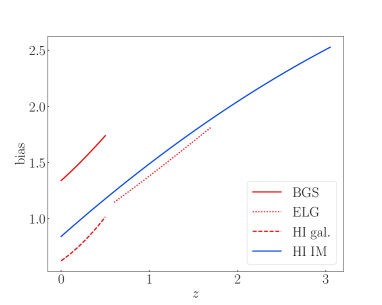
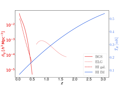
Figure 1: Left: Fiducial clustering bias for galaxy (red) and intensity mapping (blue) samples. Right: Comoving number density for galaxy surveys (red, left $y$-axis) and brightness temperature for IM surveys (blue, right $y$-axis)

There is shot noise in HI IM surveys – but on the linear scales that we consider, this shot noise is much smaller than the thermal noise (see below) and can be safely neglected [37, 36].

For the cross-power spectra, the cross shot-noise may be neglected if the overlap of halos hosting the two samples is negligible. This is shown to be the case for BGS $\times$ IM in [26] (see also [38]). We assume that it is a reasonable approximation in the cases ELG $\times$ IM and BGS $\times$ HI galaxies, so that $P_{gH}^{\rm shot}\approx 0\approx P_{gg^{\prime}}^{\rm shot}$. (Note that we do not consider the multi-tracer case HI galaxies $\times$ HI IM.)

The thermal noise in HI IM depends on the sky temperature in the radio band, the survey specifications and the array configuration (single-dish or interferometer). For the single-dish mode of SKAO-like IM surveys, the thermal noise power spectrum is [39, 40, 41]:

$$P_{H\!H}^{\mathrm{therm}}(z)=\frac{\Omega_{\mathrm{sky}}}{2\nu_{21}t_{\mathrm{tot}}}\,\frac{(1+z)^{2}r(z)^{2}}{H(z)}\,\left[\frac{T_{\mathrm{sys}}(z)}{\bar{T}_{H}(z)}\right]^{2}\,\frac{1}{N_{\rm d}}\,,$$ (2.13)

where $\nu_{21}=1420\,\mathrm{MHz}$ is the rest-frame frequency of the 21 cm emission, $t_{\mathrm{tot}}$ is the total observing time, and the number of dishes is $N_{\mathrm{d}}=197$ (with dish diameter $D_{\mathrm{d}}=15\,$m). The system temperature is modelled as [42]:

$$T_{\mathrm{sys}}(z)=T_{\rm d}(z)+T_{\rm sky}(z)=T_{\rm d}(z)+2.7+25\bigg{[}\frac{400\,\mathrm{MHz}}{\nu_{21}}(1+z)\bigg{]}^{2.75}~{}\mathrm{K},$$ (2.14)

where $T_{\rm d}$ is the dish receiver temperature given in [26]. The total signal is then

$$\tilde{P}_{H\!H}(z,k,\mu)=P_{H\!H}(z,k,\mu)+P_{H\!H}^{\mathrm{therm}}(z)\,.$$ (2.15)

2.3 Intensity mapping beam and foregrounds

HI IM surveys in single-dish mode have poor angular resolution, which results in power loss on small transverse scales, i.e. for large $k_{\perp}=(1-\mu^{2})^{1/2}k$. This effect is typically modelled by a Gaussian beam factor [39]:

$${\cal D}_{\rm beam}(z,k,\mu)=\exp\left[-\frac{(1-\mu^{2})k^{2}r(z)^{2}\theta_{\rm b}(z)^{2}}{16\ln 2}\right]\quad\mbox{with}\quad\theta_{\rm b}(z)=1.22\,\frac{\lambda_{21}(1+z)}{D_{\rm d}}\,.$$ (2.16)

HI IM surveys are also contaminated by foregrounds much larger than the HI signal. Since these foregrounds are spectrally smooth, they can be separated from the non-smooth signal on small to medium scales. However, on very large radial scales, i.e. for small $k_{\|}=\mu k$, the signal becomes smoother and therefore, the separation fails. A comprehensive treatment requires simulations of foreground cleaning of the HI signal (e.g. [43, 44]). For a simplified Fisher forecast, we can instead use a foreground avoidance approach by excising the regions of Fourier space where the foregrounds are significant. This means removing large radial scales, which can be modelled by the foreground-avoidance factor:

$$\mathcal{D}_{\mathrm{fg}}(k,\mu)=\Theta\left(\left|k_{\|}\right|-k_{\mathrm{fg}}\right)=\begin{cases}1,&\left|k_{\|}\right|>k_{\mathrm{fg}}\\ 0,&\left|k_{\|}\right|\leq k_{\mathrm{fg}}\end{cases}$$ (2.17)

where $\Theta$ is the Heaviside step function. We assume the cut is made at a minimum value of

$$k_{\mathrm{fg}}=0.01\,h\,\mathrm{Mpc}^{-1}\,.$$ (2.18)

In summary, the HI IM density contrast is modified by beam and foreground effects as follows:

$$\Delta_{H}(z,k,\mu)~{}~{}\to~{}~{}\mathcal{D}_{\rm beam}(z,k,\mu)\,\mathcal{D}_{\mathrm{fg}}(k,\mu)\,\Delta_{H}(z,k,\mu)\,.$$ (2.19)

3 Multi-tracer Fisher Analysis

The Fisher matrix in each redshift bin for the combination of two dark matter tracers is [45, 46]

$$F_{\alpha\beta}^{\bm{P}}=\sum_{\mu=-1}^{+1}\,\sum_{k=k_{\mathrm{min}}}^{k_{\mathrm{max}}}\,\partial_{\alpha}\,\bm{P}\cdot\mathrm{Cov}(\bm{P},\bm{P})^{-1}\cdot\partial_{\beta}\,\bm{P}^{\mathrm{T}}\;,$$ (3.1)

where $\partial_{\alpha}=\partial\,/\,\partial\vartheta_{\alpha}$, with $\vartheta_{\alpha}$ the parameters, and $\bm{P}$ is the data vector of the power spectra:

$$\bm{P}=\big{(}P_{gg}\,,\,{P}_{gH}\,,\,{P}_{H\!H}\big{)}\quad\mbox{or}~{}~{}\big{(}P_{gg}\,,\,{P}_{gg^{\prime}}\,,\,{P}_{g^{\prime}g^{\prime}}\big{)}\;.$$ (3.2)

Note that the sum over $\mu$ incorporates the foreground avoidance via the Heaviside factor (2.17) in $P_{HA}$. Also note that $\bm{P}$ contains no noise terms – these appear in the covariance below. The reason is that noise does not depend on the cosmological parameters. Although the thermal noise in HI IM depends on $H$, this arises from mapping the Gaussian pixel noise term to Fourier space.

The multi-tracer covariance includes the shot and thermal noises, and is given by [22, 24, 45, 46]:

$$\mathrm{Cov}(\bm{P},\bm{P})=\frac{k_{\rm f}^{3}}{2\pi k^{2}\Delta k}\,\frac{2}{\Delta\mu}\,\begin{pmatrix}\tilde{P}_{gg}^{2}&&\tilde{P}_{gg}\tilde{P}_{gH}&&\tilde{P}_{gH}^{2}\\ &&&&\\ \tilde{P}_{gg}\tilde{P}_{gH}&&\frac{1}{2}\big{[}\tilde{P}_{gg}\tilde{P}_{H\!H}+\tilde{P}_{gH}^{2}\big{]}&&\tilde{P}_{H\!H}\tilde{P}_{gH}\\ &&&&\\ \tilde{P}_{gH}^{2}&&\tilde{P}_{H\!H}\tilde{P}_{gH}&&\tilde{P}_{H\!H}^{2}\end{pmatrix}\;,$$ (3.3)

and similarly for the case $g\times g^{\prime}$. Here $\Delta k$ and $\Delta\mu$ are bin-widths and the fundamental mode $k_{\mathrm{f}}$, corresponding to the longest wavelength, is determined by the comoving survey volume of the redshift bin centred at $z$:

$$V(z)=\frac{\Omega_{\mathrm{sky}}}{3}\bigg{[}r\Big{(}z+\frac{\Delta z}{2}\Big{)}^{3}-r\Big{(}z-\frac{\Delta z}{2}\Big{)}^{3}\bigg{]}=\bigg{[}\frac{2\pi}{k_{\mathrm{f}}(z)}\bigg{]}^{3}\;.$$ (3.4)

We choose the bin-widths following [47, 48, 49]:

$$\Delta z=0.1,~{}~{}\Delta\mu=0.04,~{}~{}\Delta k=k_{\mathrm{f}}\;.$$ (3.5)

In order to exclude the small length scales that are beyond the validity of linear perturbation theory, we impose a conservative maximum wavenumber of $.08h/$Mpc at $z=0$, with a redshift evolution as proposed in [50]:

$$k_{\mathrm{max}}(z)=0.08\,(1+z)^{2/(2+n_{s})}\;h\,\mathrm{Mpc}^{-1}\;.$$ (3.6)

The largest length scale that can be measured in galaxy surveys corresponds to the smallest wavenumber, given by

$$k_{\mathrm{min}}=k_{\mathrm{f}}\,.$$ (3.7)

For HI IM surveys, $k_{\mathrm{min}}=\text{max}\big{(}k_{\mathrm{f}},k_{\mathrm{fg}}\big{)}$.

The multi-tracer Fisher matrix applies for a perfectly overlapping region in both redshift range and sky area for the two tracers. If the samples differ in redshift and sky area, then we can add the independent non-overlapping Fisher matrix information of the individual surveys. The full Fisher matrix, denoted by $g\otimes H$, is [26, 51]

$$F_{\alpha\beta}^{g\otimes H}=F_{\alpha\beta}^{\bm{P}}(\text{overlap})+F_{\alpha\beta}^{g}(\text{non-overlap})+F_{\alpha\beta}^{H}(\text{non-overlap})\;,$$ (3.8)

and similarly for the case $g\otimes g^{\prime}$.

For the cosmological parameters, we choose $\sigma_{8,0}$, $\Omega_{b,0}$, $\Omega_{c,0}$, $n_{s}$ and $h$, since we are focusing on constraining the growth rate index $\gamma$, which should be minimally affected by the remaining $\Lambda$CDM parameters on linear scales. We fix these remaining cosmological parameters to their Planck 2018 best-fit values [52]. We therefore consider the following set of cosmological parameters together with the two nuisance bias parameters:

$$\vartheta_{\alpha}=\big{(}\gamma,\,\sigma_{8,0},\,n_{s},\,h,\,\Omega_{b0},\,\Omega_{c0}\,;\,b_{A0}\big{)}\quad\mbox{where}~{}~{}A=\mbox{BGS, ELG, HIg, IM1, IM2}\;.$$ (3.9)

The marginalised errors are then obtained as

$$\sigma\big{(}\vartheta_{\alpha}\big{)}=\Big{[}\big{(}F^{-1}\big{)}_{\alpha\alpha}\Big{]}^{1/2}\;.$$ (3.10)

We compute numerically the Fisher derivatives with respect to $n_{s}$, $h$, $\Omega_{b0}$ and $\Omega_{c0}$, using the 5-point stencil approximation with selected step sizes, shown in Table 2. The derivatives are stable for $0.0003\leq\mbox{step size}\leq 0.1$ [27]. The derivatives with respect to $\gamma$, $\sigma_{8,0}$ and $b_{A0}$ are computed analytically, with for example

$$\frac{1}{P_{AA}}\,\partial_{\gamma}P_{AA}=\frac{2\mu^{2}\,\Omega_{m}^{\gamma}\,\ln\Omega_{m}}{b_{A}+\mu^{2}\,\Omega_{m}^{\gamma}}\,.$$ (3.11)

Table 2: Numerical step sizes for Fisher derivatives.

Parameters	$n_{s}$	$h$	$\Omega_{b0}$	$\Omega_{c0}$
Optimal step size	0.1	0.01	0.01	0.02

4 Results

Figure 2–Figure 4 show the 1$\sigma$ error contours for the parameter $\gamma$ and the cosmological parameters, after marginalising over the 2 bias nuisance parameters in (3.9). There are significant degeneracies, which the multi-tracer partly alleviates, allowing for improved precision on the cosmological parameters. The improvement is small, unlike the case of the growth index, which shows significant improvement. This is not surprising, since the multi-tracer removes cosmic variance from the effective bias, i.e. the clustering bias plus the RSD contribution, as shown in [21]. All multi-tracer pairs show a significant reduction in errors on $\gamma$ compared to the best single tracer. The improvements are shown in the fractional errors listed in Table 3. We note that these multi-tracer errors are obtained using only linear scales.

For the BGS and HI galaxy combination in Figure 2, the multi-tracer fractional error on $\gamma$ is less than half of the BGS value. We note that our constraint on $\gamma$ for the single-tracer BGS is weaker than that in [26]. The reason is that [26] uses the angular power spectra with a large number of very thin redshift bins (width 0.01) and considers all possible cross-bin correlations. By contrast, our standard Fourier analysis only uses 5 redshift bins of width 0.1, and does not include cross-correlations between different redshift bins. The single-tracer HI galaxy delivers the weakest constraints, mainly due to its smaller sky area and number density.

Table 3: Fractional errors $\sigma(\vartheta_{\alpha})/\vartheta_{\alpha}$.

Sample	$\gamma$	$\sigma_{8,0}$	$n_{s}$	$h$	$\Omega_{b0}$	$\Omega_{c0}$
BGS	0.467	0.169	0.319	0.465	0.523	0.105
ELG	0.119	0.018	0.066	0.102	0.107	0.020
HI gal.	0.664	0.25	0.921	1.445	1.586	0.239
IM Band 2.	0.217	0.067	0.225	0.353	0.391	0.059
IM Band 1.	0.061	0.013	0.050	0.077	0.084	0.018
BGS $\otimes$ HI gal.	0.228	0.096	0.295	0.465	0.520	0.089
BGS $\otimes$ IM Band 2	0.139	0.048	0.168	0.267	0.278	0.052
ELG $\otimes$ IM Band 1	0.047	0.008	0.037	0.057	0.062	0.013

When BGS is combined with HI IM Band 2 (Figure 3) the situation changes. HI IM Band 2 gives much better constraints than BGS, with an error on $\gamma$ less than half of the BGS error. This arises despite the effects of foreground noise because HI IM Band 2 covers a much larger area of the sky, which results in more Fourier modes that contribute to the Fisher analysis. In addition, foreground noise affects the largest scales where the $\gamma$ is not strong. When IM surveys are combined with spectroscopic galaxy surveys, the impact of foreground noise on the multi-tracer constraints is further mitigated. Table 3 shows that the multi-tracer error on $\gamma$ is reduced by $\sim 40\%$ compared to the best single-tracer error from HI IM Band 2.

The best $\gamma$ precision is delivered at high redshifts by ELG $\otimes$ IM  Band 1 (Figure 4). The IM Band 1 error on $\gamma$ is $\sim 6\%$ while ELG produces about double this error. The multi-tracer reduces the error to $\sim 5\%$.

Table 4: Fractional errors on bias parameters.

Survey	Sample	${b_{A0}}$	${b_{B0}}$
$g$ (DESI-like)	BGS	0.1719	-
	ELG	0.0169	-
$g$ (SKAO-like)	HI gal.	0.2691	-
$H$ (SKAO-like)	IM Band 2	0.0696	-
	IM Band 1	0.0138	-
$g\otimes g^{\prime}$	BGS $\otimes$ HI gal.	0.0997	0.0989
$g\otimes H$	BGS $\otimes$ IM Band 2	0.0501	0.0496
	ELG $\otimes$ IM Band 1	0.0083	0.0085

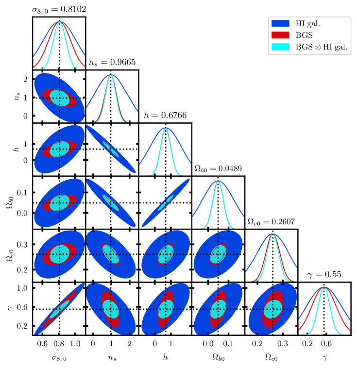
Figure 2: Marginal 1$\sigma$ contours for $\gamma$ and cosmological parameters, from the BGS and HI galaxy combination.

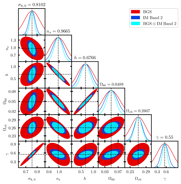
Figure 3: As in Figure 2, from the BGS and HI IM Band 2 combination.

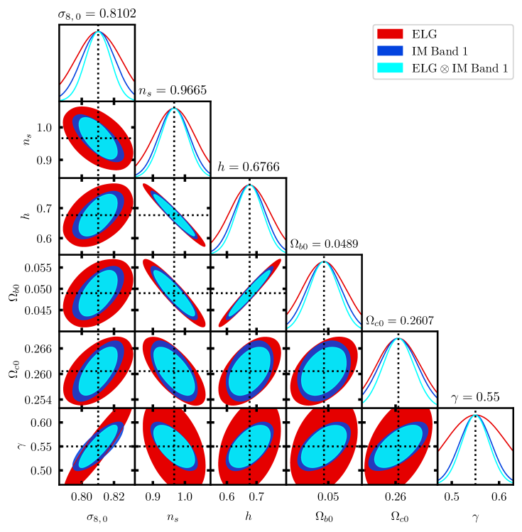
Figure 4: As in Figure 2, from the ELG and HI IM Band 1 combination.

Table 4 displays the fractional errors for the 2 bias nuisance parameters for the 3 survey combinations. The multi-tracer constraints on bias nuisance parameters are much tighter than those obtained from the individual single-tracers (compare [19, 26]).

All of our constraints are obtained from scales $k<k_{\rm max}$ where linear perturbations are accurate. In Figure 5 we investigate the effect on the marginalised fractional error for $\gamma$ of changing $k_{\rm max,0}$ from its value given in (3.6). The plots confirm that constraints are sensitive to $k_{\mathrm{max,0}}$. We would unnecessarily lose information by reducing our $k_{\rm max,0}$ value. On the other hand, increasing it leads to higher precision – but at the risk of moving into the regime of nonlinear effects – especially in RSD – which requires much more effort to model. The multi-tracer has the advantage of allowing us to avoid these difficulties while at the same time delivering constraints that would not be possible with single tracers in the linear regime.

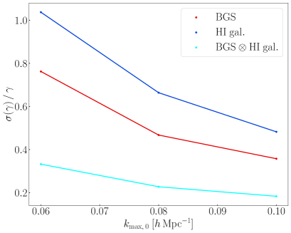
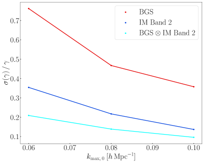
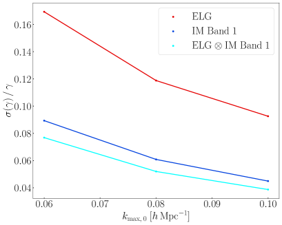
Figure 5: Change in fractional errors on $\gamma$ as a function of $k_{\rm max,0}$, for the BGS and HI galaxy (top left), BGS and HI IM Band 2 (top right) and ELG and HI IM Band 1 (bottom) samples. Our choice is $k_{\rm max,0}=0.08\,h$/Mpc.

5 Conclusion

Using a simplified Fisher analysis we have estimated the multi-tracer constraints on the growth rate of large-scale structure, for pairs of tracer samples that are similar to those expected from the specifications of SKAO and DESI surveys. The multi-tracer is known to be more effective, the more different are the pairs of surveys – and this motivates our choice of DESI-like and SKAO-like samples.

We applied a foreground-avoidance filter to the HI intensity mapping samples and included the effects of the radio telescope beam, but we have not dealt with the many other systematics. Our aim is not a realistic forecast for specific surveys, but rather a proof of principle analysis to answer the question: what is the potential of the multi-tracer to improve constraints using only linear scales?

By confining the signal to linear scales, we avoid the highly complex modelling, especially for RSD, that is required to access nonlinear scales. The cross-power spectra represent an additional complexity in the nonlinear regime [24]. Our Fisher analysis suggests that significant improvements in precision on the growth rate could be achieved by multi-tracing next-generation radio-optical pairs of samples. The details are summarised qualitatively in Figure 2, Figure 3 and Figure 4, and quantitatively in Table 3. The biggest improvements, $\sim 40-60\%$, are for the low-redshift pairs.

This indicates that it is worthwhile to perform a more realistic analysis and derive more realistic forecasts. We leave this for further work. Finally, we note that multi-tracer improvements can be delivered without requiring additional observational resources.

Acknowledgements We are supported by the South African Radio Astronomy Observatory (SARAO) and the National Research Foundation (Grant No. 75415).

References

- [1] T. Clifton, P. G. Ferreira, A. Padilla, and C. Skordis, Modified Gravity and Cosmology, Phys. Rept. 513 (2012) 1–189, [arXiv:1106.2476].
- [2] K. Koyama, Cosmological Tests of Modified Gravity, Rept. Prog. Phys. 79 (2016), no. 4 046902, [arXiv:1504.04623].
- [3] D. Langlois, Dark energy and modified gravity in degenerate higher-order scalar–tensor (DHOST) theories: A review, Int. J. Mod. Phys. D 28 (2019), no. 05 1942006, [arXiv:1811.06271].
- [4] N. Frusciante and L. Perenon, Effective field theory of dark energy: A review, Phys. Rept. 857 (2020) 1–63, [arXiv:1907.03150].
- [5] G.-B. Zhao et al., The clustering of the SDSS-IV extended Baryon Oscillation Spectroscopic Survey DR14 quasar sample: a tomographic measurement of cosmic structure growth and expansion rate based on optimal redshift weights, Mon. Not. Roy. Astron. Soc. 482 (2019), no. 3 3497–3513, [arXiv:1801.03043].
- [6] E. V. Linder, Cosmic growth history and expansion history, Phys. Rev. D 72 (2005) 043529, [astro-ph/0507263].
- [7] EUCLID Collaboration, R. Laureijs et al., Euclid Definition Study Report, arXiv:1110.3193.
- [8] X. Chen, The Tianlai project: a 21cm cosmology experiment, Int. J. Mod. Phys. Conf. Ser. 12 (2012) 256–263, [arXiv:1212.6278].
- [9] R. A. Battye, M. L. Brown, I. W. A. Browne, R. J. Davis, P. Dewdney, C. Dickinson, G. Heron, B. Maffei, A. Pourtsidou, and P. N. Wilkinson, BINGO: a single dish approach to 21cm intensity mapping, arXiv:1209.1041.
- [10] L. B. Newburgh et al., HIRAX: A Probe of Dark Energy and Radio Transients, Proc. SPIE Int. Soc. Opt. Eng. 9906 (2016) 99065X, [arXiv:1607.02059].
- [11] DESI Collaboration, A. Aghamousa et al., The DESI Experiment Part I: Science,Targeting, and Survey Design, arXiv:1611.00036.
- [12] MeerKLASS Collaboration, M. G. Santos et al., MeerKLASS: MeerKAT Large Area Synoptic Survey, in MeerKAT Science: On the Pathway to the SKA, 9, 2017. arXiv:1709.06099.
- [13] SKA Collaboration, D. J. Bacon et al., Cosmology with Phase 1 of the Square Kilometre Array: Red Book 2018: Technical specifications and performance forecasts, Publ. Astron. Soc. Austral. 37 (2020) e007, [arXiv:1811.02743].
- [14] N. Sailer, E. Castorina, S. Ferraro, and M. White, Cosmology at high redshift — a probe of fundamental physics, JCAP 12 (2021), no. 12 049, [arXiv:2106.09713].
- [15] P. Bull, Extending cosmological tests of General Relativity with the Square Kilometre Array, Astrophys. J. 817 (2016), no. 1 26, [arXiv:1509.07562].
- [16] L. Amendola et al., Cosmology and fundamental physics with the Euclid satellite, Living Rev. Rel. 21 (2018), no. 1 2, [arXiv:1606.00180].
- [17] A. Pourtsidou, D. Bacon, and R. Crittenden, HI and cosmological constraints from intensity mapping, optical and CMB surveys, Mon. Not. Roy. Astron. Soc. 470 (2017), no. 4 4251–4260, [arXiv:1610.04189].
- [18] E. Castorina and M. White, Measuring the growth of structure with intensity mapping surveys, JCAP 06 (2019) 025, [arXiv:1902.07147].
- [19] J. Fonseca, J.-A. Viljoen, and R. Maartens, Constraints on the growth rate using the observed galaxy power spectrum, JCAP 1912 (2019), no. 12 028, [arXiv:1907.02975].
- [20] U. Seljak, Extracting primordial non-gaussianity without cosmic variance, Phys. Rev. Lett. 102 (2009) 021302, [arXiv:0807.1770].
- [21] P. McDonald and U. Seljak, How to measure redshift-space distortions without sample variance, JCAP 10 (2009) 007, [arXiv:0810.0323].
- [22] M. White, Y.-S. Song, and W. J. Percival, Forecasting Cosmological Constraints from Redshift Surveys, Mon. Not. Roy. Astron. Soc. 397 (2008) 1348–1354, [arXiv:0810.1518].
- [23] C. Blake et al., Galaxy And Mass Assembly (GAMA): improved cosmic growth measurements using multiple tracers of large-scale structure, Mon. Not. Roy. Astron. Soc. 436 (2013) 3089, [arXiv:1309.5556].
- [24] G.-B. Zhao et al., The completed SDSS-IV extended Baryon Oscillation Spectroscopic Survey: a multitracer analysis in Fourier space for measuring the cosmic structure growth and expansion rate, Mon. Not. Roy. Astron. Soc. 504 (2021), no. 1 33–52, [arXiv:2007.09011].
- [25] C. Adams and C. Blake, Joint growth rate measurements from redshift-space distortions and peculiar velocities in the 6dF Galaxy Survey, Mon. Not. Roy. Astron. Soc. 494 (2020), no. 3 3275–3293, [arXiv:2004.06399].
- [26] J.-A. Viljoen, J. Fonseca, and R. Maartens, Constraining the growth rate by combining multiple future surveys, JCAP 09 (2020) 054, [arXiv:2007.04656].
- [27] S. Yahia-Cherif, A. Blanchard, S. Camera, S. Casas, S. Ilić, K. Markovic, A. Pourtsidou, Z. Sakr, D. Sapone, and I. Tutusaus, Validating the Fisher approach for stage IV spectroscopic surveys, Astron. Astrophys. 649 (2021) A52, [arXiv:2007.01812].
- [28] DESI Collaboration, D. J. Schlegel et al., A Spectroscopic Road Map for Cosmic Frontier: DESI, DESI-II, Stage-5, arXiv:2209.03585.
- [29] M. Berti, M. Spinelli, and M. Viel, Multipole expansion for 21 cm intensity mapping power spectrum: Forecasted cosmological parameters estimation for the SKA observatory, Mon. Not. Roy. Astron. Soc. 521 (2023), no. 3 3221–3236, [arXiv:2209.07595].
- [30] D. Blas, J. Lesgourgues, and T. Tram, The Cosmic Linear Anisotropy Solving System (CLASS) II: Approximation schemes, JCAP 1107 (2011) 034, [arXiv:1104.2933].
- [31] L. Wolz, C. Tonini, C. Blake, and J. S. B. Wyithe, Intensity Mapping Cross-Correlations: Connecting the Largest Scales to Galaxy Evolution, Mon. Not. Roy. Astron. Soc. 458 (2016), no. 3 3399–3410, [arXiv:1512.04189].
- [32] C. J. Anderson et al., Low-amplitude clustering in low-redshift 21-cm intensity maps cross-correlated with 2dF galaxy densities, Mon. Not. Roy. Astron. Soc. 476 (2018), no. 3 3382–3392, [arXiv:1710.00424].
- [33] A. Rubiola, S. Cunnington, and S. Camera, Baryon acoustic oscillations from HI intensity mapping: the importance of cross-correlations in the monopole and quadrupole, arXiv:2111.11347.
- [34] N. Agarwal, V. Desjacques, D. Jeong, and F. Schmidt, Information content in the redshift-space galaxy power spectrum and bispectrum, JCAP 03 (2021) 021, [arXiv:2007.04340].
- [35] G. Jelic-Cizmek, F. Lepori, C. Bonvin, and R. Durrer, On the importance of lensing for galaxy clustering in photometric and spectroscopic surveys, JCAP 04 (2021) 055, [arXiv:2004.12981].
- [36] F. Villaescusa-Navarro et al., Ingredients for 21 cm Intensity Mapping, Astrophys. J. 866 (2018), no. 2 135, [arXiv:1804.09180].
- [37] E. Castorina and F. Villaescusa-Navarro, On the spatial distribution of neutral hydrogen in the Universe: bias and shot-noise of the HI power spectrum, Mon. Not. Roy. Astron. Soc. 471 (2017), no. 2 1788–1796, [arXiv:1609.05157].
- [38] S. Casas, I. P. Carucci, V. Pettorino, S. Camera, and M. Martinelli, Constraining gravity with synergies between radio and optical cosmological surveys, Phys. Dark Univ. 39 (2023) 101151, [arXiv:2210.05705].
- [39] P. Bull, P. G. Ferreira, P. Patel, and M. G. Santos, Late-time cosmology with 21cm intensity mapping experiments, Astrophys. J. 803 (2015), no. 1 21, [arXiv:1405.1452].
- [40] D. Alonso, P. G. Ferreira, M. J. Jarvis, and K. Moodley, Calibrating photometric redshifts with intensity mapping observations, Phys. Rev. D 96 (2017), no. 4 043515, [arXiv:1704.01941].
- [41] S. Jolicoeur, R. Maartens, E. M. De Weerd, O. Umeh, C. Clarkson, and S. Camera, Detecting the relativistic bispectrum in 21cm intensity maps, JCAP 06 (2021) 039, [arXiv:2009.06197].
- [42] Cosmic Visions 21 cm Collaboration, R. Ansari et al., Inflation and Early Dark Energy with a Stage II Hydrogen Intensity Mapping experiment, arXiv:1810.09572.
- [43] S. Cunnington, S. Camera, and A. Pourtsidou, The degeneracy between primordial non-Gaussianity and foregrounds in 21 cm intensity mapping experiments, Mon. Not. Roy. Astron. Soc. 499 (2020), no. 3 4054–4067, [arXiv:2007.12126].
- [44] M. Spinelli, I. P. Carucci, S. Cunnington, S. E. Harper, M. O. Irfan, J. Fonseca, A. Pourtsidou, and L. Wolz, SKAO HI intensity mapping: blind foreground subtraction challenge, Mon. Not. Roy. Astron. Soc. 509 (2021), no. 2 2048–2074, [arXiv:2107.10814].
- [45] A. Barreira, On the impact of galaxy bias uncertainties on primordial non-Gaussianity constraints, JCAP 12 (2020) 031, [arXiv:2009.06622].
- [46] D. Karagiannis, R. Maartens, J. Fonseca, S. Camera, and C. Clarkson, Multi-tracer power spectra and bispectra: Formalism, arXiv:2305.04028.
- [47] D. Karagiannis, A. Lazanu, M. Liguori, A. Raccanelli, N. Bartolo, and L. Verde, Constraining primordial non-Gaussianity with bispectrum and power spectrum from upcoming optical and radio surveys, Mon. Not. Roy. Astron. Soc. 478 (2018), no. 1 1341–1376, [arXiv:1801.09280].
- [48] V. Yankelevich and C. Porciani, Cosmological information in the redshift-space bispectrum, Mon. Not. Roy. Astron. Soc. 483 (2019), no. 2 2078–2099, [arXiv:1807.07076].
- [49] R. Maartens, S. Jolicoeur, O. Umeh, E. M. De Weerd, C. Clarkson, and S. Camera, Detecting the relativistic galaxy bispectrum, JCAP 03 (2020), no. 03 065, [arXiv:1911.02398].
- [50] VIRGO Consortium Collaboration, R. E. Smith, J. A. Peacock, A. Jenkins, S. D. M. White, C. S. Frenk, F. R. Pearce, P. A. Thomas, G. Efstathiou, and H. M. P. Couchmann, Stable clustering, the halo model and nonlinear cosmological power spectra, Mon. Not. Roy. Astron. Soc. 341 (2003) 1311, [astro-ph/0207664].
- [51] S. Jolicoeur, R. Maartens, and S. Dlamini, Constraining primordial non-Gaussianity by combining next-generation galaxy and 21 cm intensity mapping surveys, Eur. Phys. J. C 83 (2023), no. 4 320, [arXiv:2301.02406].
- [52] Planck Collaboration, N. Aghanim et al., Planck 2018 results. VI. Cosmological parameters, Astron. Astrophys. 641 (2020) A6, [arXiv:1807.06209]. [Erratum: Astron.Astrophys. 652, C4 (2021)].