Resilient Intraparticle Entanglement and its Manifestation in
Spin Dynamics of Disordered Dirac Matter

Abstract

Topological quantum matter exhibits novel transport phenomena driven by entanglement between internal degrees of freedom, as for instance generated by spin-orbit coupling effects. Here we report on a direct connection between the mechanism driving spin relaxation and the intertwined dynamics between spin and sublattice degrees of freedom in disordered graphene. Beyond having a direct observable consequence, such intraparticle entanglement is shown to be resilient to disorder, pointing towards a novel resource for quantum information processing.

The study of quantum transport in topological quantum matter and quantum materials is a central topic of modern condensed matter, given its connection to an emerging class of nontrivial phenomena and materials including topologically protected edge states, exotic Moiré physics, twisted multilayers of 2D materials, and strongly correlated systems Giustino et al. (2021). Particularly relevant is the existence of the variety of internal degrees of freedom which arise from lattice symmetry and internal degeneracies, such as A/B sublattice pseudospin or $\mathbf{K}_{+}/\mathbf{K}_{-}$ valley isospin in graphene, or layer pseudospin in multilayer systems assembled by stacking (and twist angle) engineering. The contributions of spin-orbit coupling, magnetic exchange fields and Coulomb interactions further yield nontrivial modifications of intraparticle and interparticle entanglement properties as well as the formation of strongly correlated and topological states, which result in a wealth of puzzling and exotic phenomena including superconductivity and orbital magnetism Andrei et al. (2021); Tian et al. (2023).

In this wide context, exploration of the dynamics of internal degrees of freedom and their intertwined evolution is particularly relevant when a connection can be made with some directly accessible experimental observable. The case of graphene has been particularly scrutinized given the longstanding debate concerning the nature of the spin transport and spin relaxation mechanisms at play Ertler et al. (2009); Huertas-Hernando et al. (2009); Ochoa et al. (2012); Zhang and Wu (2012); Pi et al. (2010); Han and Kawakami (2011); McCreary et al. (2012); Zomer et al. (2012); Kochan et al. (2014); Soriano et al. (2015); Drögeler et al. (2016); Thomsen et al. (2015); Van Tuan et al. (2016); Cummings and Roche (2016); Gebeyehu et al. (2019), while entanglement effects on weak localization Sousa et al. (2022) or spin-orbit torque phenomena Dueñas et al. have also been discussed recently. The peculiar dynamics of intraparticle entanglement between spin and sublattice in massless Dirac fermions, generated by spin-orbit coupling, have been argued to explain the energy dependence of spin lifetime in graphene Tuan et al. (2014), and may offer a novel resource of quantum information given its magnitude and resilience to state preparation in the ultraclean limit de Moraes et al. (2020), as well as complement other possible entanglement mechanisms Kindermann (2009); Bittencourt and Bernardini (2017). However, to date the dynamics and robustness of such intraparticle entanglement in the presence of disorder remains to be explored. Additionally, a direct connection between entanglement and the spin lifetime in graphene has yet to be elucidated.

In this Letter, we use numerical simulations to study the dynamics of spin and intraparticle entanglement in disordered graphene. We consider two types of disorder – charge impurities and magnetic impurities – and in both cases we find that the entanglement saturates to a finite value, independent of the initial state and the type or strength of disorder. This spin-sublattice entanglement thus appears to be an equilibrium property of graphene, with a magnitude that is robust to charge and spin scattering. For future proposals to use such intraparticle entanglement as a quantum resource, these results suggest that disorder may not be an inherently limiting factor.

Additionally, we derive an expression that directly relates the intraparticle entanglement to the Elliott-Yafet mechanism of spin relaxation in graphene. In the absence of magnetic impurities, this mechanism is dominant at low doping, yielding a minimum in the spin lifetime at the charge neutrality point. Our results therefore offer a direct, experimentally observable consequence of the innate spin-sublattice entanglement in graphene, and suggest that this connection could be used to monitor quantum information, as well as be generalized to other entanglement phenomena in similar materials.

Electronic model and measure of entanglement — To study its entanglement properties, we consider a continuum model of graphene near the $\mathbf{K}_{\pm}$ points with Rashba spin-orbit coupling (SOC) induced by a perpendicular electric field or a substrate Rashba (2009); Sierra et al. (2021). The Hamiltonian is

$$\hat{H}(\mathbf{k}) =\hbar v_{\mathrm{F}}\left(\nu\hat{\sigma}_{x}k_{x}+\hat{\sigma}_{y}k_{y}\right)\otimes\hat{s}_{0}$$

$$+\lambda_{\mathrm{R}}\left(\nu\hat{\sigma}_{x}\otimes\hat{s}_{y}-\hat{\sigma}_{y}\otimes\hat{s}_{x}\right),$$ (1)

where $v_{\mathrm{F}}$ is the Fermi velocity, $\nu=\pm 1$ is the valley index, $\mathbf{k}$ is the crystalline momentum with respect to the $\mathbf{K}_{\pm}$ points, $\lambda_{\mathrm{R}}$ is the Rashba SOC strength and $\hat{\mathrm{s}}_{i}$ ($\hat{\mathrm{\sigma}}_{i}$) are the Pauli matrices in the spin (sublattice) space. In this work, without loss of generality, we restrict ourselves to one valley, $\nu=+1$. The eigenenergies of the system are $\varepsilon_{\pm}^{\xi}(\mathbf{k})=\xi\left(\pm\lambda_{\mathrm{R}}+\sqrt{\lambda_{\mathrm{R}}^{2}+\varepsilon_{0}^{2}}\right)$, where $\xi=+1\,(-1)$ for electrons (holes) and $\varepsilon_{0}=\hbar v_{\mathrm{F}}|\mathbf{k}|$ is the energy dispersion in absence of SOC. The eigenstates of the Hamiltonian, in the sublattice-spin basis $\left\{A_{\uparrow},A_{\downarrow},B_{\uparrow},B_{\downarrow}\right\}$, are given by

$$\ket{\varepsilon^{\xi}_{\pm}(\mathbf{k})}=\dfrac{1}{\sqrt{N_{\pm}}}\begin{bmatrix}e^{-i\theta}&\pm i\gamma_{\pm}&\xi\gamma_{\pm}&\pm\xi ie^{i\theta}\end{bmatrix}^{\mathrm{T}},$$ (2)

where $\theta=\atan(k_{y}/k_{x})$ is the direction of momentum in the graphene plane, $\gamma_{\pm}=\varepsilon_{\pm}/\varepsilon_{0}$ and $N_{\pm}=2(1+\gamma_{\pm}^{2})$.

The spin-sublattice entanglement of an arbitrary state $\ket{\psi}$ can be quantified using the concurrence $C_{\psi}$ Wootters (1998). For pure states this is computed as

$$C_{\psi}=|\braket{\psi}{\widetilde{\psi}}|=|\bra{\psi}\left(\hat{\sigma}_{Y}\otimes\hat{\sigma}_{Y}\right)\ket{\psi^{*}}|,$$ (3)

where $\ket{\widetilde{\psi}}$ denotes the spin-flip transformation of $\ket{\psi}$ and $\hat{\sigma}_{Y}=\begin{bmatrix}0&-i\\ i&0\end{bmatrix}$ in spin space. The concurrence is a so-called entanglement monotone, equal to 0 for separable states and 1 for maximally entangled states. Applying its definition to Eq. (2), we find that the concurrence of the eigenstates is $C_{\varepsilon}=\lambda_{\mathrm{R}}/\sqrt{\varepsilon_{0}^{2}+\lambda_{\mathrm{R}}^{2}}$.

Therefore, the eigenstates of graphene in the presence of Rashba SOC are maximally entangled at the charge neutrality point ($\varepsilon_{0}=0$) and become separable for higher doping, with $C_{\varepsilon}$ decaying as $\sim$$1/\varepsilon_{0}$. On the other hand, increasing the Rashba coupling will increase the entanglement for a given Fermi energy ($E_{\mathrm{F}}$). In general, the concurrence is a monotonically-increasing function of $x=\lambda_{\mathrm{R}}/E_{\mathrm{F}}$, given by $C_{\varepsilon}=x/\sqrt{1+x^{2}}$, where we have let $E_{\mathrm{F}}\approx\varepsilon_{0}$. The purple solid line in Fig. 1 shows precisely this behavior.

Entanglement dynamics in the presence of disorder — In a previous work, we examined the dynamics of intraparticle spin-sublattice entanglement in perfectly clean graphene de Moraes et al. (2020). Here we examine the dynamics and robustness of such intraparticle entanglement in the presence of disorder. To do so, we have implemented a single-particle Monte Carlo method that tracks the concurrence and spin of a quantum state as it undergoes free flight and scattering in the presence of different types of disorder (schematically shown in Fig. 1, right inset). Our approach follows the general procedure for semiclassical Monte Carlo simulation of semiconductors Jacoboni and Reggiani (1983) (details in the Supplemental Material sup ). We consider the time evolution of a state at a given $E_{\mathrm{F}}$ either in the presence of charge impurities which randomize the momentum direction at every scattering event, or magnetic impurities which randomize the spin orientation. The impurity density is related to the scattering time, $\tau$, which is a free parameter in our simulations. Finally, we consider a large number of trajectories to calculate the ensemble average of the spin and concurrence as they evolve in time.

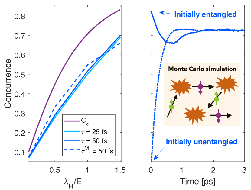
Figure 1: Left panel: Long-time concurrence for different scattering times in the presence of charge impurities (solid blue lines) and magnetic impurities (dashed blue line). The solid purple line indicates the concurrence of the eigenstates of the system. Right panel: Concurrence dynamics for the initial states $\ket{\psi_{\mathrm{entan}}}$ (solid line) and $\ket{\psi_{\mathrm{sep}}}$ (dash-dotted line) in the presence of charge impurities. The inset shows a schematic of the semiclassical Monte Carlo simulation. Independent of the initial state, type of scattering, or impurity density, the concurrence saturates to a universal finite value.

Some examples of the ensemble concurrence dynamics in the presence of charge impurities are shown in the right panel of Fig. 1. We have considered two different initial states: one fully separable, $\ket{\psi_{\mathrm{sep}}}=\frac{1}{\sqrt{2}}\left[1\,0\,1\,0\right]^{\mathrm{T}}=\frac{1}{\sqrt{2}}\left(\ket{A}+\ket{B}\right)\otimes\ket{\uparrow}$ and one highly entangled Bell-type state, $\ket{\psi_{\mathrm{entan}}}=\frac{1}{\sqrt{2}}\left[1\,0\,0\,1\right]^{\mathrm{T}}=\frac{1}{\sqrt{2}}\left(\ket{A}\otimes\ket{\uparrow}+\ket{B}\otimes\ket{\downarrow}\right)$. In both cases, the concurrence converges to a finite and universal value at long times. This behavior is independent of the type of disorder and the initial state. In the left panel of Fig. 1, we show the converged value of the concurrence as a function of $x=\lambda_{\mathrm{R}}/E_{\mathrm{F}}$. The solid blue lines correspond to charge impurity scattering with $\tau=25$ and $50$ fs. Meanwhile, the blue dashed line shows the case for magnetic impurities with $\tau=50$ fs. Notably, all three curves fall on top of each other, indicating that the intraparticle entanglement appears to be robust and universal in the presence of disorder in graphene.

Fig. 1 (left panel) shows that the converged value of concurrence grows monotonically with $\lambda_{\mathrm{R}}/E_{\mathrm{F}}$. This scaling behavior follows that of the eigenstates themselves, whose concurrence is shown by the solid purple line. The final concurrence arises from a linear combination of both bands at $E_{\mathrm{F}}$, and thus will generally be smaller than the concurrence of each indidividual eigenstate. Nonetheless, these results demonstrate a general picture of entanglement dynamics, with the initial nonequilibrium entanglement relaxing to an equilibrium value determined by the concurrence of the eigenstates. This is analogous to the spin in a magnetic system relaxing to an equilibrium value determined by the net magnetization Kittel (2004).

Spin relaxation time — Next we examine the features of the spin relaxation time of out-of-plane spins and directly relate it to the concurrence of the graphene eigenstates. The spin relaxation time, $\tau_{\mathrm{s}}$, is obtained from the Monte Carlo simulations by fitting the average value of the out-of-plane spin polarization to either an exponential decay, $\braket{\hat{s}_{z}}=\exp(-t/\tau_{\mathrm{s}})$, or an oscillating exponential, $\braket{\hat{s}_{z}}=\exp(-t/\tau_{\mathrm{s}})\cos(2\pi t/T_{\Omega})$. We use the former when the spin precession time, $T_{\Omega}=\pi\hbar/\lambda_{\mathrm{R}}$, is longer than the scattering time and the latter when $T_{\Omega}<\tau$. The solid green curve in the inset of Fig. 2 shows an example of the spin dynamics from the Monte Carlo simulations when $T_{\Omega}\gg\tau$, and the dashed green line is the fit to an exponential decay.

In the main panel of Fig. 2, we plot the spin relaxation time as a function of the Fermi energy for different values of the scattering time. As in Fig. 1, the solid curves are for charge impurity scattering and the dashed curve is for magnetic impurities. The scattering times are given in the legend, and the Rashba SOC strength is $\lambda_{\mathrm{R}}=500$ $\upmu$eV. The spin precession time is then $T_{\Omega}=\pi\hbar/\lambda_{\mathrm{R}}=4.1$ ps, much longer than all values of $\tau$ that we consider.

For charge impurity scattering, at low energies $\tau_{\mathrm{s}}$ scales quadratically with $E_{\mathrm{F}}$ and is proportional to $\tau$. This is consistent with the Elliott-Yafet (EY) mechanism of spin relaxation, which in graphene was predicted to scale as $\tau_{\mathrm{s}}^{\mathrm{EY}}\propto(E_{\mathrm{F}}/\lambda_{\mathrm{R}})^{2}\tau$ Ochoa et al. (2012). At higher energies, when $\tau_{\mathrm{s}}^{\mathrm{EY}}$ becomes large, the spin dynamics are dominated by the D’yakonov-Perel (DP) mechanism, and the spin lifetime scales inversely with the scattering time, $\tau_{\mathrm{s}}^{\mathrm{DP}}=(\hbar/2\lambda_{\mathrm{R}})^{2}/\tau$ Ertler et al. (2009). This crossover between the EY and the DP regime happens at $E_{\mathrm{F}}\approx\hbar/\tau$.

In the case of scattering by magnetic impurities, $\tau_{\mathrm{s}}=\tau$ for all energies, as shown by the dashed line in Fig. 2. This arises from the fact that magnetic impurities directly randomize the spin at each scattering event.

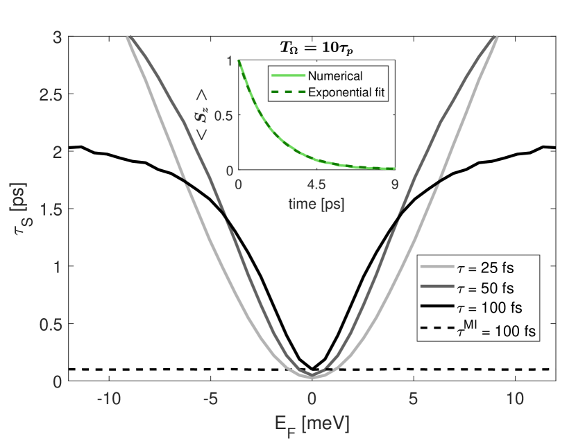
Figure 2: Main panel: spin relaxation time for different scattering times for charge impurities (solid lines) and magnetic impurities (dashed line). Inset: out-of-plane spin dynamics obtained from the Monte Carlo simulations (solid green line) and a fit to an exponential decay (dashed green line).

As seen in Fig. 2, at low energies the spin lifetime is dominated by EY relaxation, where $\tau_{s}\propto(E_{\mathrm{F}}/\lambda_{\mathrm{R}})^{2}$. Meanwhile, above we noted that the concurrence of the eigenstates scales approximately inversely with energy, $C_{\varepsilon}\approx(E_{\mathrm{F}}/\lambda_{\mathrm{R}})^{-1}$. In the following we demonstrate that there is a direct link between spin-sublattice entanglement and EY spin relaxation in graphene.

To derive an expression for EY spin relaxation in graphene, we start with the general interpretation of the mechanism – that at every momentum scattering event, the spin polarization is reduced due to mixing of spin up and spin down states Žutić et al. (2004). We define a spin loss coefficient that describes the relative amount of spin lost during the $n$th scattering event,

$$\mathcal{S}^{n,n-1}\equiv\dfrac{\braket{\hat{s}_{z}^{n}}}{\braket{\hat{s}_{z}^{n-1}}},$$ (4)

where $\braket{\hat{s}_{z}^{n-1}}$ is the ensemble spin polarization just before the $n$th scattering event and $\braket{\hat{s}_{z}^{n}}$ is the ensemble spin polarization just after. After a time $t$, the spin polarization will then be given by $\braket{\hat{s}_{z}(t)}=\mathcal{S}^{N,N-1}\,\,...\,\,\ \mathcal{S}^{2,1}\mathcal{S}^{1,0}\braket{\hat{s}_{z}^{0}}$, where $t=N\tau$ with $\tau$ the average scattering interval. Assuming that every spin loss coefficient is equal, $\mathcal{S}^{n,n-1}\approx\mathcal{S}$, the net spin lost during an average interval $\tau$ is $\braket{\hat{s}_{z}(t+\tau)}-\braket{\hat{s}_{z}(t)}=-(1-\mathcal{S})\braket{\hat{s}_{z}(t)}$, giving

$$\frac{\mathrm{d}\braket{\hat{s}_{z}(t)}}{\mathrm{d}t}\approx-\frac{1-\mathcal{S}}{\tau}\braket{\hat{s}_{z}(t)}.$$ (5)

This yields an exponential decay of the spin polarization, $\braket{\hat{s}_{z}(t)}=\braket{\hat{s}_{z}^{0}}\exp(-t/\tau_{\mathrm{s}})$, with spin lifetime

$$\tau_{\mathrm{s}}^{\mathrm{EY}}=\frac{\tau}{1-\mathcal{S}}.$$ (6)

To explicitly calculate $\mathcal{S}$, we start by considering the spin lost by a single particle during a single scattering event. Before a scattering event, the state of a particle with momentum $\mathbf{k}$ can be written as a linear combination of the graphene+Rashba eigenstates, $\ket{\psi(\mathbf{k})}=\sum_{\xi\nu}\beta_{\xi\nu}\ket{\varepsilon_{\nu}^{\xi}(\mathbf{k})}$. For $E_{\mathrm{F}}>0$ $(E_{\mathrm{F}}<0)$, this projection is over the conduction (valence) band eigenstates. The spin polarization of this state is $\braket{\hat{s}_{z}^{\psi}(\mathbf{k})}\equiv\braket{\psi(\mathbf{k})}{\hat{s}_{z}}{\psi(\mathbf{k})}$. A charge impurity scattering event changes $\mathbf{k}\rightarrow\mathbf{k^{\prime}}$, and thus the scattered state can be written as a projection onto the eigenstates at $\mathbf{k^{\prime}}$, $\ket{\psi(\mathbf{k^{\prime}})}=\sum_{\xi\nu}\beta_{\xi\nu}^{\prime}\ket{\varepsilon_{\nu}^{\xi}(\mathbf{k^{\prime}})}$, where $\beta_{\xi\nu}^{\prime}=\braket{\varepsilon_{\nu}^{\xi}(\mathbf{k^{\prime}})}{\psi(\mathbf{k})}$, with proper normalization. The spin polarization of this scattered state is $\braket{\hat{s}_{z}^{\psi}(\mathbf{k^{\prime}})}=\braket{\psi(\mathbf{k^{\prime}})}{\hat{s}_{z}}{\psi(\mathbf{k^{\prime}})}$, and the spin loss in this particular scattering event is thus $\mathcal{S}_{\psi}(\mathbf{k}-\mathbf{k^{\prime}})=\braket{\hat{s}_{z}^{\psi}(\mathbf{k^{\prime}})}/\braket{\hat{s}_{z}^{\psi}(\mathbf{k})}$. Finally, the average spin loss per scattering event, $\mathcal{S}$, is the average of $\mathcal{S}_{\psi}(\mathbf{k}-\mathbf{k^{\prime}})$ over all $\mathbf{k}-\mathbf{k^{\prime}}$, accounting for the form of $\ket{\psi}$ after a large number of scattering events. By calculating $\mathcal{S}$ in this way, we then obtain the EY spin relaxation time by applying Eq. (6).

Following this procedure (see SM for details sup ), we arrive at the following expression for EY spin relaxation in graphene with Rashba SOC,

$$\tau_{\mathrm{s}}^{\mathrm{EY}}=\dfrac{3-C_{\varepsilon}^{4}}{5C_{\varepsilon}^{2}-3C_{\varepsilon}^{4}}\,\tau.$$ (7)

This expression, with explicit dependence on the concurrence of the graphene eigenstates, can be broken down into two regimes. At high energies, when $C_{\varepsilon}\approx\lambda_{\mathrm{R}}/E_{\mathrm{F}}\ll 1$, Eq. (7) reduces to $\tau_{\mathrm{s}}^{\mathrm{EY}}\approx(3/5)(1/C_{\varepsilon})^{2}\tau\approx(3/5)(E_{\mathrm{F}}/\lambda_{\mathrm{R}})^{2}\tau$. This is the usual EY relation in graphene Ochoa et al. (2012). On the other hand, for low energies when $E_{\mathrm{F}}\lesssim\lambda_{\mathrm{R}}$ and thus $C_{\varepsilon}\approx 1$, the EY relation becomes $\tau_{\mathrm{s}}^{\mathrm{EY}}\approx\tau$. In this regime, when there is only one band at $E_{\mathrm{F}}$, every scattering event changes the spin.

The full scaling of $\tau_{\mathrm{s}}^{\mathrm{EY}}$ with Fermi energy is shown in Fig. 3 (right axis). The black circles are EY spin relaxation times extracted from the Monte Carlo simulations, while the solid black line corresponds to Eq. (7), showing perfect agreement. On the left axis, we show the concurrence of the eigenstates, highlighting the inverse correlation between the spin-sublattice entanglement and EY spin relaxation in graphene.

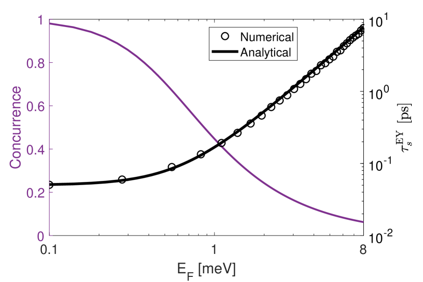
Figure 3: Numerical and analytical spin relaxation times due to the EY mechanism (black, right axis), along with the concurrence (purple, left axis), as a function of the Fermi energy. The numerical results are from the Monte Carlo simulations, while the analytical spin lifetime is given by Eq. (7).

Conclusions — Using Monte Carlo simulations, we have revealed the nature of spin-sublattice entanglement dynamics in disordered graphene. We find that this intraparticle entanglement evolves to a universal value that is determined by the eigenstates of graphene and is independent of the initial state, and of the type and strength of disorder. These results suggest that potential applications of this intraparticle entanglement as a resource may not be inherently limited by disorder.

Next, we have derived an explicit relation between Elliott-Yafet spin relaxation and the spin-sublattice entanglement in graphene. When spin relaxation is driven by spin-orbit coupling, the EY mechanism is dominant at low doping, yielding a minimum of spin lifetime at the charge neutrality point. Thus, the behavior of spin transport at low doping in graphene may be a direct experimental signature of the quantum entanglement properties of the charge carriers.

Beyond spin-sublattice entanglement, similar experimental features may arise from interparticle sublattice entanglement between electrons and holes in single-layer graphene Kindermann (2009), or sublattice-layer entanglement in bilayer graphene Bittencourt and Bernardini (2017). Looking ahead, the complex interplay between intraparticle and interparticle entanglement remains to be explored, with this work laying the groundwork for understanding such dynamics. Beyond the quantification of entanglement through experimental data, such studies may be used to envision novel schemes of data processing and storage that utilize the multiple internal degrees of freedom of quantum matter.