Bound states and point interactions of the one-dimensional pseudospin-one Hamiltonian

Abstract

The spectrum of a one-dimensional pseudospin-one Hamiltonian with a three-component potential is studied for two configurations: (i) all the potential components are constants over the whole coordinate space and (ii) the profile of some components is of a rectangular form. In case (i), it is illustrated how the structure of three (lower, middle and upper) bands depends on the configuration of potential strengths including the appearance of flat bands at some special values of these strengths. In case (ii), the set of two equations for finding bound states is derived. The spectrum of bound-state energies is shown to depend crucially on the configuration of potential strengths. Each of these configurations is specified by a single strength parameter $V$. The bound-state energies are calculated as functions of the strength $V$ and a one-point approach is developed realizing correspondent point interactions. For different potential configurations, the energy dependence on the strength $V$ is described in detail, including its one-point approximation. From a whole variety of bound-state spectra, four characteristic types are singled out.

Keywords: Points interactions, bound states, flat bands, Dirac equation

1 Introduction

Experimental discovery of graphene attracted attention to condensed matter systems with spectrum of quasiparticles similar to the relativistic one. It is well known that quasiparticle excitations in graphene are described at low energies by the massless Dirac equation in two space dimensions. Moreover, it was shown [1] that more complicated fermionic quasiparticles could be realized in crystals with special space groups with no analogues in particle physics, where the Poincaré symmetry provides strong restrictions allowing only three types: Dirac, Weyl and Majorana (not discovered yet) particles with spin 1/2. In condensed matter systems, besides fermions with pseudospin 1/2, other fermions with a higher pseudospin can appear in two- and three-dimensional solids. In particular, special attention is paid to fermionic excitations with pseudospin one, whose Hamiltonian is given by the scalar product of momentum and the spin-1 matrices [2, 3, 4].

Many aspects of pseudospin-1 Hamiltonians, such as the energy spectrum having a flat band along with two dispersive bands which are linear in momentum as in graphene, are fascinating. The dice model is an example of such a system, which hosts pseudospin-1 fermions with a completely flat band at zero energy [2, 3]. The quenching of the kinetic energy in flat bands strongly enhances the role of electron-electron and other interactions and may lead to the realization of many very interesting correlated states such as ferromagnetism [5], superconductivity in twisted bilayer graphene [6] and plethora of other quantum phases [7].

Currently, a whole body of literature has been accumulated, which is devoted to the investigation of physical quantities in the presence of flat bands in two-dimensional systems such as orbital susceptibility [3], optical conductivity [8, 9, 10], magnetotransport [11, 12], RKKY [13, 14] and Coulomb [15, 16] interactions. However, one-dimensional pseudospin-1 systems have been much less studied. Here, one should note the recent works by Zhang with coauthors [17, 18, 19], where the bound state problem in a one-dimensional pseudospin-1 Dirac Hamiltonian with a flat band was investigated in the presence of delta- and square well potentials. In particular, the existence of infinite series of bound states near the flat band appears to be of great interest [18]. Very recently, the transport properties and snake states of pseudospin-1 Dirac-like electrons have been analyzed by Jakubský and Zelaya [20, 21] in Lieb lattice under barrier- and well-like electrostatic interactions.

In the present work we consider a one-dimensional spin-1 Hamiltonian $H=H_{0}+V(x)$ with its free-particle part

$$\!\!\!\!\!\!\!\!H_{0}=-{\rm i}S_{y}{d\over dx}+mS_{z}\,,~{}~{}S_{y}={1\over\sqrt{2}}\left(\begin{array}[]{lll}0~{}-{\rm i}~{}~{}~{}0\\ {\rm i}~{}~{}~{}~{}0~{}-{\rm i}\\ 0~{}~{}~{}~{}{\rm i}~{}~{}~{}~{}0\end{array}\right),~{}~{}S_{z}=\left(\begin{array}[]{lll}1~{}~{}~{}0~{}~{}~{}~{}0\\ 0~{}~{}~{}0~{}~{}~{}~{}0\\ 0~{}~{}~{}0~{}\!-1\end{array}\right)$$ (1)

and a potential

$$V(x)=\left(\begin{array}[]{ccc}V_{11}(x)~{}~{}~{}~{}~{}~{}0~{}~{}~{}~{}~{}~{}~{}~{}~{}~{}\,0\\ ~{}~{}~{}0~{}~{}~{}~{}~{}~{}~{}V_{22}(x)~{}~{}~{}~{}~{}~{}\,0\\ ~{}~{}~{}~{}~{}~{}~{}\,0~{}~{}~{}~{}~{}~{}~{}~{}~{}~{}0~{}~{}~{}~{}~{}~{}~{}~{}V_{33}(x)\end{array}\right).$$ (2)

We use the matrix $S_{y}$ instead of $S_{x}$ in [18] in order to have real coefficients in the equations as the Dirac equation in the Majorana representation.

Let $\psi(x)={\rm col}\!\left(\psi_{1}(x),\,\psi_{2}(x),\,\psi_{3}(x)\right)$ be a three-component wave function. Then the Schrödinger equation $\left[H_{0}+V(x)\right]\psi(x)=E\psi(x)$ with energy $E$ is represented in the component form as the system of three equations:

$$\begin{array}[]{lll}\vskip 3.0pt plus 1.0pt minus 1.0pt-\,\psi^{\prime}_{2}(x)/\sqrt{2}+\left[m+V_{11}(x)\right]\psi_{1}(x)\!&=&\!E\psi_{1}(x),\\ \vskip 3.0pt plus 1.0pt minus 1.0pt\left[\psi^{\prime}_{1}(x)-\psi^{\prime}_{3}(x)\right]/\sqrt{2}+V_{22}(x)\psi_{2}(x)\!&=&\!E\psi_{2}(x),\\ \psi^{\prime}_{2}(x)/\sqrt{2}-\left[m-V_{33}(x)\right]\psi_{3}(x)\!&=&\!E\psi_{3}(x)\,,\end{array}$$ (3)

where the prime stands for the differentiation over $x$. Notice that adding the first and third equations we get an algebraic relation between the functions $\psi_{1}$ and $\psi_{3}$. In fact, we have two differential equations and one algebraic constraint. This is due to the fact that the matrix $S_{y}$ is singular, ${\rm det}S_{y}=0$, and its rank equals two. Thus the system (3) cannot be transformed to the canonical form $\dot{\psi}_{i}=M_{ij}\psi_{j}$ for the system of differential equations.

The free-particle spectrum of equations (3), where $V_{11}(x)=V_{22}(x)=V_{33}(x)\equiv 0$, consists of the three bands:

$$\!\!\!\!\!\!\!\!\!\!\!\!\!\!\!\!\!\!\!\!\!\!\!\!\!\!\!\!E=0~{}(\mbox{flat band}),~{}E=\pm\sqrt{k^{2}+m^{2}}~{}(\mbox{upper and lower dispersion bands}).$$ (4)

The gap in this spectrum consists of the two intervals $-m<E<0$ and $0<E<m$ where possible bound states can exist in the presence of a potential term. The spectrum of the Hamiltonian $H_{0}$ is particle-hole symmetric with the isolated flat band at zero energy, which is a consequence of the existence of a matrix $C$,

$$C=\left(\begin{array}[]{ccc}0&0&1\\ 0&1&0\\ 1&0&0\end{array}\right),$$ (8)

that anti-commutes with $H_{0}$. It is interesting that, for another type of the mass term $m\,{\rm diag}(1,-1,1)$, the flat band with the energy $E=m$ exists and touches either the upper ($m>0$) or the lower ($m<0$) dispersive energy band, thus violating the particle-hole symmetry (similar to the two-dimensional $\alpha-{\cal T}_{3}$ model [22, 15]).

While in the non-relativistic case, in the presence of an external constant potential, the free-particle spectrum is simply shifted accordingly, the spectrum of system (3), in a similar situation where the strength components $(V_{11}$, $V_{22}$ and $V_{33})$ are constant over the whole $x$-axis, depends on the configuration of these components in a non-trivial way. Therefore it is of interest to examine the spectrum structure of a pseudospin-1 Hamiltonian depending on all the vectors ${\rm col}(V_{11},\,V_{22},\,V_{33})$ which forms a three-dimensional space ${\mathbb{R}}^{3}$. The further task is to single out explicitly in this space the sets of the existence of flat bands.

For realizing bound states of the pseudospin-one Hamiltonian, the components $V_{11}(x)$, $V_{22}(x)$ and $V_{33}(x)$, defined as functions on the whole $x$-axis, must decay to zero at $|x|\to\infty$. Then the bound states (if any) are expected to appear within the gap $-m<E<m$. Having the explicit solution of equations (3) with constant strength components, it is reasonable to choose the components of the potential $V(x)$ in the form of rectangles (barriers or wells). In simple terms, such rectangular potentials describe a heterostructure composed of parallel plane layers. The particle motion in these systems is confined only along the $x$-axis, being free in (perpendicular) planes. In this case, for some special configurations of the strengths $V_{11}$, $V_{22}$ and $V_{33}$, it is possible to examine the bound-state spectrum in an explicit form, exhibiting a number of interesting and intriguing features.

Because of the rapid progress in fabricating nanoscale quantum devices, the investigation of extremely thin layers described by sharply localized potentials is of particular interest nowadays. In this regard, the so-called zero-range or point interaction models, which are widely used in various applications to quantum physics [23, 24, 25, 26], should also be elaborated for Dirac-like systems. In general, a point interaction, being a singular object, is determined by the two-sided boundary conditions on a wave function, which are given at the point of singularity (say, e.g., $x=\pm 0$). In the case of a heterostructure consisting of a finite number of parallel layers, it is quite useful to apply the transfer matrix approach as a starting point to implement such a modeling. Knowing the matrix that connects the values of a wave function and its derivative (in the non-relativistic case) or the components of a spinor (in the relativistic case) given at the boundaries of each mono-layer, the full transfer matrix of the system can easily be calculated as the product of all the mono-layer matrices. The further step is to shrink the thickness of the full multi-layered system to zero. For example, in this way, the exactly solvable model has been constructed for the non-relativistic Schrödinger equation with a delta derivative potential $\delta^{\prime}(x)$ [27, 28]. In other studies, performed for instance in [29], the squeezing limit This squeezed …may be applied separately to each layer, fixing the distances between the layers. Here, using the transfer matrix method, the bound states of a one-dimensional Dirac equation with multiple delta potentials have been studied. Based on this method, for a similar equation written in a more general form, the continuity between the states of perfect transmission and bound states has been established in [30].

Finally, it should be emphasized that the squeezed connection matrices, which define the corresponding point interactions, depend on the shape of the functions used for the squeezing limit realization. This non-uniqueness problem refers to both the non-relativistic Schrödinger equation with a $\delta^{\prime}$-like potential [31, 32, 33] and the relativistic Dirac equation with a $\delta$-potential [29]. In this regard, the piecewise representation of the potential profile of layers seems to be motivated from a physical point of view because of satisfying the principle of strength additivity [29].

2 Three-band structure of the energy spectrum for the Hamiltonian with constant potentials

Consider the system for which $V_{jj}(x)\equiv V_{jj}=$ const., $V_{jj}\in{\mathbb{R}}$, $j=1,2,3$, and rewrite equations (3) in the form

$$\begin{array}[]{ccc}\vskip 3.0pt plus 1.0pt minus 1.0pt-\,\psi^{\prime}_{2}(x)&=&\sqrt{2}\,(E-V_{1})\psi_{1}(x),\\ \vskip 3.0pt plus 1.0pt minus 1.0pt\psi^{\prime}_{1}(x)-\psi^{\prime}_{3}(x)&=&\sqrt{2}\,(E-V_{2})\psi_{2}(x),\\ \vskip 3.0pt plus 1.0pt minus 1.0pt\psi^{\prime}_{2}(x)&=&\sqrt{2}\,(E-V_{3})\psi_{3}(x),\end{array}$$ (9)

where

$$V_{1}:=V_{11}+m,~{}~{}~{}V_{2}\equiv V_{22}\,,~{}~{}~{}V_{3}:=V_{33}-m$$ (10)

are renormalized potentials strengths (or intensities).

Assume that $\psi(k;x)={\rm col}\!\left(A_{1},\,A_{2},\,A_{3}\right)\exp(\pm{\rm i}kx)$ with unknowns $A_{j}$’s and a wave number $k$ being real or imaginary. Inserting this representation into equations (9), we get a system of three linear equations. Calculating next the determinant of this system, we arrive at the equation

$$\!\!\!\!\!\!\!\!\!\!\!\!\!\!\!\!\!\!\!\!\!F(E)=G(E)k^{2},~{}~{}~{}k^{2}\in{\mathbb{R}}\setminus\{0\},\;\;G(E)=E-V_{a}\,,~{}~{}~{}V_{a}:={1\over 2}\left(V_{1}+V_{3}\right),$$ (11)

where the function $F(E)$ has a cubic factorized form:

$$F(E)=(E-V_{1})(E-V_{2})(E-V_{3})$$ (12)

Cubic equation (11) with (12) determines the dispersion laws that describe the relation between the energy $E$ and the wave number $k$. Explicit solutions can be written using the well-known formulas for the roots of this cubic equation, but we prefer a qualitative analysis of the equation, which we will consider in the next section.

A general solution of equations (9) can be found if we express the constants $A_{1}$ and $A_{3}$ through $A_{2}$, using also equation (11). As a result, it can be represented as the sum of linearly independent solutions:

$$\psi(k;x)=B_{1}\,{\rm col}\left(-\sigma_{1},\,1,\,\sigma_{3}\right){\rm e}^{{\rm i}kx}+B_{2}\,{\rm col}\left(\sigma_{1},\,1,\,-\sigma_{3}\right){\rm e}^{-{\rm i}kx},$$ (13)

where the constants $B_{1}$ and $B_{2}$ are arbitrary,

$$\sigma_{j}:={{\rm i}k\over\sqrt{2}\,(E-V_{j})}\,,\quad j=1,3,$$ (14)

and the wave number $k$, being real or imaginary, is related to the energy $E$ through the formula

$$k=\sqrt{(E-V_{1})(E-V_{2})(E-V_{3})\over E-V_{a}}\,.$$ (15)

2.1 Structure of dispersion and flat bands

For the analysis of the three-band spectrum $E=E(k)$, where $k$ is real, it is convenient to use the diagrams shown in figure 1.

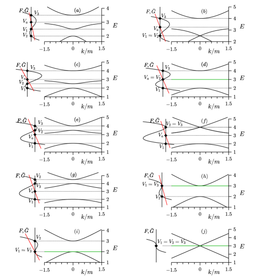
Figure 1: Three (dispersive and flat) bands for different ‘positions’ of strength $V_{2}$ with respect to strengths $V_{1}$, $V_{3}$ ($V_{1}\leq V_{3}$) and their middle value $V_{a}$ , while successive ‘lifting’ from bottom to top along $E$-axis: (a) $-\infty<V_{2}<V_{1}$, (b) $V_{2}=V_{1}$, (c) $V_{1}<V_{2}<V_{a}$, (d) $V_{2}=V_{a}$, (e) $V_{a}<V_{2}<V_{3}$, (f) $V_{2}=V_{3}$, (g) $V_{3}<V_{2}<\infty$, (h) $-\infty<V_{2}<V_{1}=V_{3}$, (i) $V_{1}=V_{3}<V_{2}<\infty$, (j) $V_{2}=V_{1}=V_{3}$. Left diagrams in each panel represent both sides of dispersion equation (11), $F=F(E)$ (black curves) and $\bar{G}=G(E)k^{2}$ (red straight lines). Green horizontal lines in panels (d) and (h)–(j) represent flat bands.

Here, without loss of generality, it is assumed that $V_{1}\leq V_{3}$. The solutions for the energy $E$ are indicated by the points of intersection of the cubic function $F(E)$ and the straight line $G(E)k^{2}$ that passes through the middle point $V_{a}$ located between the zeroes $E=V_{1}$ and $E=V_{3}$. The slope of this line is governed by $k^{2}>0$ and rotating it around the ‘turning’ point $V_{a}$, one obtains the energy bands $E(k)$. ‘Moving’ the zero $E=V_{2}$ of the cubic function $F(E)$ along the $E$-axis, the all possible types of the three-band spectrum $E(k)$ are visually illustrated by the right diagrams in each panel. Each type consists of the lower and upper dispersive bands, whereas the middle band can be either dispersive or flat. Thus, in panels (a)–(c) and (e)–(g) for the case $V_{1}<V_{3}$, we have the middle bands of the dispersive type, which are bounded. Here, in the limits as $V_{2}\nearrow V_{a}$ or $V_{2}\searrow V_{a}$, the two-sided middle dispersion bands shrink to a flat band horizontal line continuously, as demonstrated by panel (d). Finally, the case $V_{1}=V_{3}$ is illustrated by panels (h)–(j). Here, the flat band touches the upper dispersion band if $V_{2}<V_{1}=V_{3}$, the lower one if $V_{2}>V_{1}=V_{3}$ and both the lower and upper dispersion bands if $V_{2}=V_{1}=V_{3}$.

2.2 Flat band planes

As follows from equation (11), the existence of flat bands is provided if the two equalities $F(E)=G(E)=0$ take place simultaneously. Then the dispersion law holds true regardless of the wave number $k$. In this case, the average strength $V_{a}$ must coincide with one of the zeroes $E=V_{j}$ , $j=1,\,2,\,3$, of cubic function (12). Therefore, one of the three relations

$$V_{1}+V_{3}=2V_{j}\,,~{}~{}~{}j=1,\,2,\,3,$$ (16)

is the necessary and sufficient condition for the existence of flat bands.

In the case $j=2$, the corresponding relation in (16) becomes

$$V_{11}+V_{33}=2V_{22}\,,$$ (17)

describing a plane in the $(V_{11}\,,\,V_{22}\,,\,V_{33})$-space, which we call from now on the ${\cal A}$-plane. Hence, the flat band energy on this plane is

$$E=V_{2}=V_{22}\,.$$ (18)

Particularly, on the line $V_{11}=V_{22}=V_{33}\equiv V$, the flat band energy is shifted from $E=0$ (free-particle case) to $E=V$.

In both the cases $j=1,3$, condition (16) reduces to one equation $V_{1}=V_{3}$ . Consequently, this equation together with an arbitrary $V_{2}$, i.e.,

$$V_{33}-V_{11}=2m,~{}~{}~{}V_{22}\in{\mathbb{R}},$$ (19)

defines a plane in the $(V_{11}\,,\,V_{22}\,,\,V_{33})$-space, which we call from now on the ${\cal B}$-plane. The flat band energy on this plane is

$$E=V_{1}=V_{3}=V_{11}+m=V_{33}-m.$$ (20)

In the particular case $V_{1}=V_{2}=V_{3}$ , both equations (17) and (19) are satisfied. Therefore, there exists an intersection of the planes ${\cal A}$ and ${\cal B}$ as shown in figure 2. Consequently, on the line ${\cal A}\cap{\cal B}$, we have the flat band energy

$$E=V_{1}=V_{2}=V_{3}=V_{11}+m=V_{22}=V_{33}-m.$$ (21)

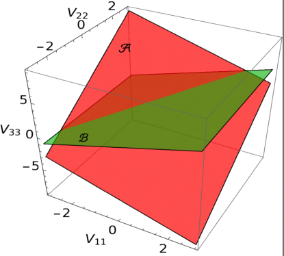
Figure 2: Intersecting flat band planes ${\cal A}$ (red plane) and ${\cal B}$ (green plane).

Thus, as illustrated by the diagrams in panels (d) and (h)–(j) of figure 1, the existence of flat bands is possible if and only if the line $G(E)k^{2}$ passes through any of zeroes $E=V_{j}$’s, $j=1,\,2,\,3$, of the cubic function $F(E)$. In the $(V_{11}\,,\,V_{22}\,,\,V_{33})$-space, the flat bands are found only on the ${\cal A}$- and ${\cal B}$-sets, including the line of their intersection ${\cal A}\cap{\cal B}$. Therefore, these sets may be called from now on as the flat band planes. One can conclude that panels (d) and (h)–(j) in figure 1 illustrate all the possible types of flat bands. In other words, any rotation of the straight (red) line around the point $E=V_{a}$ keeps the solution of equation (11) regardless of the slope determined by $k^{2}$, visualizing the existence of flat bands. Panel (d) in figure 1 describes the situation as the middle dispersion curves in panels (c) and (e) are squeezed to a (horizontal) flat line. The potential strengths in this case are found on the ${\cal A}$-plane defined by equation (17) where $V_{1}\neq V_{3}$ . The case $V_{1}=V_{3}$ but $V_{2}\neq V_{1}=V_{3}$ is presented by panels (h) and (i). As illustrated by these panels, one of the lower or upper gaps disappears in the spectrum. The potential strengths in this case belong to the ${\cal B}$-plane defined by equation (19) where $V_{2}\neq V_{1}=V_{3}$ . Finally, if $V_{1}=V_{2}=V_{3}$ , the strengths are found on the intersection of the ${\cal A}$- and ${\cal B}$-planes and, as demonstrated by panel (j), both the gaps in the spectrum disappear.

2.3 Eigenenergies and eigenfunctions of dispersion bands

In general, if $V_{1}\neq V_{3}$ and $V_{a}\neq V_{j}$ , $j=1,\,2,\,3$, the situation is illustrated by panels (a)–(c) and (e)–(g) in figure 1, where all the three [lower $E_{-}(k)$, middle $E_{0}(k)$ and upper $E_{+}(k)$] bands are dispersive. In this case, the eigenenergies $E_{\pm}(k)$ and $E_{0}(k)$ are three roots of cubic equation (11). In other cases, when the average strength $V_{a}$ coincides with one the strengths $V_{j}$’s, cubic equation (11) reduces to a quadratic form and the triad $(V_{11},\,V_{22},\,V_{33})\in{\mathbb{R}}^{3}$ falls into one of the ${\cal A}$- and ${\cal B}$-planes or their intersection.

Plane ${\cal A}$: On the ${\cal A}$-plane, owing to relation (17), the energy of the upper and lower dispersion bands is a solution of the equation $(E-V_{1})(E-V_{3})=k^{2}$. Explicitly, this solution reads

$$E=E^{A}_{\pm}(k)=E^{A}_{0}\pm\sqrt{k^{2}+\left({V_{1}-V_{3}\over 2}\right)^{\!\!2}}\,,\quad E^{A}_{0}=V_{2}\,,$$ (22)

illustrated by panel (d) in figure 1, where the energies of the lower and upper dispersion bands $E^{A}_{\pm}(k)$ are depicted by the black curves and the energy of the flat band $E^{A}_{0}$ by the blue horizontal line. Both the lower ($V_{1}<E<E_{0}^{A}$) and upper ($E_{0}^{A}<E<V_{3}$) gaps are non-empty. The corresponding three eigenfunctions $\psi_{\pm}^{A}(k;x)$ and $\psi_{0}^{A}(k;x)$ are described by general solution (13), where $\sigma_{1}$ and $\sigma_{3}$ are substituted by

$$\!\!\!\!\!\!\!\!\!\!\!\!\!\!\!\!\!\!\!\!\!\!\!\!\!\!\sigma^{A}_{1,\pm}(k)={{\rm i}\over\sqrt{2}\,k}\left[{V_{1}-V_{3}\over 2}\pm\sqrt{k^{2}+\left({V_{1}-V_{3}\over 2}\right)^{\!\!2}}\,\right],~{}~{}\sigma_{1,0}^{A}(k)={{\rm i}\over\sqrt{2}\,k}(V_{2}-V_{3}),$$

(23)

$$\!\!\!\!\!\!\!\!\!\!\!\!\!\!\!\!\!\!\!\!\!\!\!\!\!\!\sigma^{A}_{3,\pm}(k)={{\rm i}\over\sqrt{2}\,k}\left[{V_{3}-V_{1}\over 2}\pm\sqrt{k^{2}+\left({V_{1}-V_{3}\over 2}\right)^{\!\!2}}\,\right],~{}~{}\sigma_{3,0}^{A}(k)={{\rm i}\over\sqrt{2}\,k}(V_{2}-V_{1}),$$

respectively.

Plane ${\cal B}$: Similarly, on the ${\cal B}$-plane, we arrive at the equation $(E-V_{1})(E-V_{2})=k^{2}$, having the solution

$$E=E^{B}_{\pm}(k)={V_{1}+V_{2}\over 2}\pm\sqrt{k^{2}+\left({V_{1}-V_{2}\over 2}\right)^{\!\!2}}\,,\quad E_{0}^{B}=V_{1}=V_{3}\,.$$ (24)

This solution is depicted in figure 1 for two configurations, where the strength $V_{2}$ does not coincide with the flat band energy $E_{0}^{B}$: in panel (h) $V_{2}<E_{0}^{B}$ and in panel (i) $V_{2}>E_{0}^{B}$. Correspondingly, only the lower gap $V_{2}<E<E_{0}^{B}$ and the upper gap $E_{0}^{B}<E<V_{2}$ are non-empty, while respectively the upper and lower gaps disappear. Similarly, the eigenfunctions $\psi_{\pm}^{B}(k;x)$ and $\psi_{0}^{B}(k;x)$ are given by wave function (13), where $\sigma_{1}$ and $\sigma_{3}$ are replaced by

$$\sigma^{B}_{1,\pm}(k)=\sigma^{B}_{3,\pm}(k)={{\rm i}\over\sqrt{2}\,k}\left[{V_{1}-V_{2}\over 2}\pm\sqrt{k^{2}+\left({V_{1}-V_{2}\over 2}\right)^{\!\!2}}\,\right],$$

(25)

$$\sigma^{B}_{1,0}(k)=\sigma^{B}_{3,0}(k)={{\rm i}\over\sqrt{2}\,k}(V_{1}-V_{2})={{\rm i}\over\sqrt{2}\,k}(V_{3}-V_{2}).$$

Line ${\cal A}\cap{\cal B}$: On the ${\cal A}\cap{\cal B}$-line, energies (22) and (24) reduce to

$$E=E_{\pm}^{A\cap B}(k)=E_{0}^{A\cap B}\pm|k|,\quad E_{0}^{A\cap B}=V_{1}=V_{2}=V_{3}\,.$$ (26)

As illustrated by panel (j) in figure 1, both the gaps for this configuration disappear. Setting in (23) and (25) $V_{1}=V_{2}=V_{3}$, we obtain

$$\!\!\!\!\!\!\!\sigma^{A\cap B}_{1,\pm}(k)=\sigma^{A\cap B}_{3,\pm}(k)=\pm\,{\rm sgn}(k){{\rm i}\over\sqrt{2}}\,,\quad\sigma^{A\cap B}_{1,0}(k)=\sigma^{A\cap B}_{3,0}(k)=0.~{}~{}$$ (27)

Finally, notice that, as follows from the general formula for energy (22), in the particular case $V_{11}=V_{22}=V_{33}\equiv V$, we have the energy shift $E=V\pm\sqrt{k^{2}+m^{2}}$ from the free-particle spectrum, similarly to the one-dimensional non-relativistic case. The components of the wave function, in this case, are as follows

$$\!\!\!\!\!\!\!\!\!\!\!\!\psi_{+}(k;x) = B_{1}\left(\begin{array}[]{ccc}m+\sqrt{k^{2}+m^{2}}\\ {\rm i}\sqrt{2}\,k\\ m-\sqrt{k^{2}+m^{2}}\end{array}\right){\rm e}^{{\rm i}kx}+B_{2}\left(\begin{array}[]{ccc}m+\sqrt{k^{2}+m^{2}}\\ -{\rm i}\sqrt{2}\,k\\ m-\sqrt{k^{2}+m^{2}}\end{array}\right){\rm e}^{-{\rm i}kx},$$ (34)

$$\!\!\!\!\!\!\!\!\!\!\!\psi_{0}(k;x) = B_{1}\left(\begin{array}[]{ccc}m\\ {\rm i}\sqrt{2}\,k\\ m\end{array}\right){\rm e}^{{\rm i}kx}+B_{2}\left(\begin{array}[]{ccc}m\\ -{\rm i}\sqrt{2}\,k\\ m\end{array}\right){\rm e}^{-{\rm i}kx},$$ (41)

$$\!\!\!\!\!\!\!\!\!\!\!\psi_{-}(k;x) = B_{1}\left(\begin{array}[]{ccc}m-\sqrt{k^{2}+m^{2}}\\ {\rm i}\sqrt{2}\,k\\ m+\sqrt{k^{2}+m^{2}}\end{array}\right){\rm e}^{{\rm i}kx}+B_{2}\left(\begin{array}[]{ccc}m-\sqrt{k^{2}+m^{2}}\\ -{\rm i}\sqrt{2}\,k\\ m+\sqrt{k^{2}+m^{2}}\end{array}\right){\rm e}^{-{\rm i}kx},$$ (48)

where $B_{1}$ and $B_{2}$ are arbitrary constants. Particularly, on the line ${\cal A}\cap{\cal B}$, where the gapless spectrum occurs, wave function components (41) are simplified to the form

$$\psi_{+}(k;x)\!\! = \!\!B_{1}\!\left(\begin{array}[]{ccc}1\\ {\rm sgn}(k)\,{\rm i}\sqrt{2}\\ -1\end{array}\right){\rm e}^{{\rm i}kx}+B_{2}\!\left(\begin{array}[]{ccc}1\\ -{\rm sgn}(k)\,{\rm i}\sqrt{2}\\ -1\end{array}\right){\rm e}^{-{\rm i}kx},$$ (55)

$$\psi_{0}(k;x)\!\! = \!\!B_{1}\!\left(\begin{array}[]{ccc}0\\ {\rm sgn}(k)\,{\rm i}\sqrt{2}\\ 0\end{array}\right){\rm e}^{{\rm i}kx}+B_{2}\!\left(\begin{array}[]{ccc}0\\ -{\rm sgn}(k)\,{\rm i}\sqrt{2}\\ 0\end{array}\right){\rm e}^{-{\rm i}kx},$$ (62)

$$\psi_{-}(k;x)\!\! = \!\!B_{1}\!\left(\begin{array}[]{ccc}-1\\ {\rm sgn}(k)\,{\rm i}\sqrt{2}\\ 1\end{array}\right){\rm e}^{{\rm i}kx}+B_{2}\!\left(\begin{array}[]{ccc}-1\\ -{\rm sgn}(k)\,{\rm i}\sqrt{2}\\ 1\end{array}\right){\rm e}^{-{\rm i}kx},$$ (69)

with arbitrary constants $B_{1}$ and $B_{2}$ .

3 Bound states of the Hamiltonian with rectangular potentials

In the previous section we have examined the solutions of system (3) with a three-component potential $V(x)=(V_{11},\,V_{22},\,V_{33})$, which is constant on the whole $x$-axis. Bound states can be materialized if the potential $V(x)$ is compactly supported on some finite interval. In this regard, we focus here on the potential components, each being of a rectangular form. More precisely, we assume

$$V(x)=\left\{\begin{array}[]{ll}\vskip 3.0pt plus 1.0pt minus 1.0pt{\rm col}(V_{11},\,V_{22},\,V_{33})&~{}\mbox{for}~{}x_{1}\leq x\leq x_{2}\,,\\ {\rm col}(0,\,0,\,0)&~{}\mbox{for}~{}(-\infty,\,x_{1})\cup(x_{2},\,\infty),\end{array}\right.$$ (70)

where the points $x_{1}$ and $x_{2}$ are arbitrary.

Within the interval $x_{1}<x<x_{2}$ , the representation of general solution (13) can also be rewritten in the terms of trigonometric functions as follows

$$\!\!\!\!\!\!\!\!\!\!\!\!\!\!\!\!\!\!\!\!\!\!\!\!\!\!\psi(x)=C_{1}\left(\begin{array}[]{ccc}\vskip 3.0pt plus 1.0pt minus 1.0pt(E-V_{1})^{-1}k\sin(kx)\\ \vskip 3.0pt plus 1.0pt minus 1.0pt\sqrt{2}\,\cos(kx)\\ \vskip 3.0pt plus 1.0pt minus 1.0pt(V_{3}-E)^{-1}k\sin(kx)\end{array}\right)+C_{2}\left(\begin{array}[]{ccc}\vskip 3.0pt plus 1.0pt minus 1.0pt(E-V_{1})^{-1}k\cos(kx)\\ \vskip 3.0pt plus 1.0pt minus 1.0pt-\sqrt{2}\,\sin(kx)\\ \vskip 3.0pt plus 1.0pt minus 1.0pt(V_{3}-E)^{-1}k\cos(kx)\end{array}\right),~{}~{}$$ (71)

where $C_{1}$ and $C_{2}$ are arbitrary constants. For realizing bound states, beyond the interval $x_{1}<x<x_{2}$, wave function (13) must decrease to zero at infinity. Setting in (13)–(15), $k={\rm i}\kappa$, $\kappa>0$, $V_{1}=m$, $V_{2}=0$ and $V_{3}=-m$, we arrive at the following finite representation of general solution (13) outside the interval $x_{1}<x<x_{2}$:

$$\psi(x)=\left\{\begin{array}[]{ll}\vskip 3.0pt plus 1.0pt minus 1.0ptD_{1}\,{\rm col}(\rho^{-1},\,\sqrt{2},\,\,\rho)\,{\rm e}^{\kappa(x-x_{1})}&\mbox{for}~{}-\infty<x\leq x_{1}\,,\\ D_{2}\,{\rm col}(\rho^{-1},\,-\sqrt{2},\,\,\rho)\,{\rm e}^{-\kappa(x-x_{2})}&\mbox{for}~{}~{}x_{2}\leq x<\infty,\end{array}\right.$$ (72)

where $D_{1}$ and $D_{2}$ are arbitrary constants,

$$\kappa:=\sqrt{m^{2}-E^{2}}\quad\mbox{and}\quad\rho:=\sqrt{m-E\over m+E}\,.$$ (73)

The four constants $C_{1}$ , $C_{2}$ and $D_{1}$ , $D_{2}$ in expressions (71) and (72) can be determined by using matching conditions imposed on the boundaries $x=x_{1}$ and $x=x_{2}$ . The requirement for continuity of all the three components of the wave function $\psi(x)$ at $x=x_{1}$ and $x=x_{2}$ leads to six equations that involve only the four constants. Therefore such matching conditions are not appropriate. However, as can be seen from the structure of system (3), it is not necessary to require the continuity of the components $\psi_{1}(x)$ and $\psi_{3}(x)$. Instead, it is sufficient to impose the continuity of $\psi_{1}(x)-\psi_{3}(x)$ and $\psi_{2}(x)$, so that the components $\psi_{1}(x)$ and $\psi_{3}(x)$, each alone, may in general be discontinuous at $x_{1}$ and $x_{2}$. Thus, from (71) and (72), we obtain the following four equations:

$$\begin{array}[]{rrrr}\vskip 3.0pt plus 1.0pt minus 1.0ptC_{1}\sin(kx_{1})+C_{2}\cos(kx_{1})&=&D_{1}/\gamma,\\ \vskip 3.0pt plus 1.0pt minus 1.0ptC_{1}\cos(kx_{1})-C_{2}\sin(kx_{1})&=&D_{1}\,,\\ \vskip 3.0pt plus 1.0pt minus 1.0ptC_{1}\sin(kx_{2})+C_{2}\cos(kx_{2})&=&D_{2}/\gamma,\\ \vskip 3.0pt plus 1.0pt minus 1.0ptC_{1}\cos(kx_{2})-C_{2}\sin(kx_{2})&=&-D_{2}\,,\end{array}$$ (74)

where $k$ is given by (15) and

$$\gamma:={\kappa\over k}\left(1-{V_{2}\over E}\right).$$ (75)

Note that the boundary conditions, imposed above on the components $\psi_{1}(x)-\psi_{3}(x)$ and $\psi_{2}(x)$ at $x=x_{1}$ and $x=x_{2}$, provide the continuity of the net current

$$j(x)=\psi^{\dagger}S_{y}\psi={{\rm i}\over\sqrt{2}}[\psi_{2}^{*}(\psi_{1}-\psi_{3})-(\psi_{1}^{*}-\psi_{3}^{*})\psi_{2}].$$ (76)

Equating the determinant of the system of equations (74) to zero, one can derive a necessary condition for the existence of bound states. In general, the solution inside the interval $x_{1}\leq x\leq x_{2}$ can be given through a matrix connecting the values of the functions $\psi_{1}(x)-\psi_{3}(x)$ and $\psi_{2}(x)$ at the boundary points $x=x_{1}$ and $x=x_{2}$. We define this connection matrix as follows

$$\!\!\!\!\!\!\!\!\!\!\left(\begin{array}[]{cc}(\psi_{1}-\psi_{3})(x_{2})\\ \psi_{2}(x_{2})\end{array}\right)=\Lambda\left(\begin{array}[]{cc}(\psi_{1}-\psi_{3})(x_{1})\\ \psi_{2}(x_{1})\end{array}\right),~{}~{}\Lambda:=\left(\begin{array}[]{ll}\lambda_{11}~{}~{}\lambda_{12}\\ \lambda_{21}~{}~{}\lambda_{22}\end{array}\right).~{}~{}~{}$$ (77)

Using then the boundary values of the components $\psi_{1}(x)-\psi_{3}(x)$ and $\psi_{2}(x)$ obtained from wave function (72) and excluding the constants $D_{1}$ and $D_{2}$, we get the equation for the bound state energy $E=E_{b}$ given in terms of the connection matrix $\Lambda$ that describes any potential profile inside the interval $x_{1}\leq x\leq x_{2}$:

$$\lambda_{11}+\lambda_{22}+{\kappa\over\sqrt{2}\,E}\lambda_{12}+{\sqrt{2}\,E\over\kappa}\lambda_{21}=0,$$ (78)

where $\kappa$ is defined in (73). In one dimension, similar equations have been established in [34, 35] for the non-relativistic Schrödinger equation and in [29] for the Dirac equation.

3.1 Explicit formula for the connection matrix $\Lambda$

In the particular case of solution (13), the connection matrix $\Lambda$ can be calculated explicitly. Indeed, using this solution on the interval $x_{1}\leq x\leq x_{2}$, we write

$$\begin{array}[]{ll}\vskip 3.0pt plus 1.0pt minus 1.0pt(\psi_{1}-\psi_{3})(x)&={\rm i}\eta\left(-B_{1}{\rm e}^{{\rm i}kx}+B_{2}{\rm e}^{-{\rm i}kx}\right),\\ ~{}~{}~{}~{}~{}~{}~{}\psi_{2}(x)&=B_{1}{\rm e}^{{\rm i}kx}+B_{2}{\rm e}^{-{\rm i}kx},\end{array}$$ (79)

with

$$\eta:=-{\rm i}(\sigma_{1}+\sigma_{3})={\sqrt{2}\over k}(E-V_{2}),$$ (80)

where $k$ is given by (15). Fixing equations (79) at $x=x_{1}$, we find from these equations the constants $B_{1}$ and $B_{2}$ and then substitute these values again into equations (79), but now fixed at $x=x_{2}$. As a result, we get the $\Lambda$-matrix in the form

$$\Lambda=\left(\begin{array}[]{cc}~{}~{}~{}\cos(kl)~{}~{}~{}~{}~{}~{}~{}\eta\sin(kl)\\ -\eta^{-1}\sin(kl)~{}~{}~{}\cos(kl)\end{array}\right),\quad l:=x_{2}-x_{1}\,,$$ (81)

where $k$ and $\eta$ are given by formulas (15) and (80), respectively.

3.2 Basic equations for bound state energies

Inserting the elements of $\Lambda$-matrix (81) into general equation (78), we obtain the equation for the energy of bound states $E=E_{b}$ in the form

$$2+\left(\gamma-{1\over\gamma}\right)\tan(kl)=0,$$ (82)

where the functions $k=k(E)$ and $\gamma(E)$ are defined by formulas (15) and (75), respectively.

Equation (82) splits into two simple equations with respect to the unknowns, which we denote from now on as $E=E^{+}$ and $E=E^{-}$. As a result, these equations read

$$\gamma=\left\{\vskip 3.0pt plus 1.0pt minus 1.0pt\begin{array}[]{ll}-\cot(kl/2)&\mbox{for}~{}~{}E=E^{+}\,,\\ ~{}~{}\tan(kl/2)&\mbox{for}~{}~{}E=E^{-}\,.\end{array}\right.$$ (83)

The solutions to these equations, where $k(E)$ and $\gamma(E)$ are given by (15) and (75), describe bound state energies $E=E^{\pm}_{b}$, the total number of which at a given three-component strength $(V_{11},\,V_{22},\,V_{33})\in{\mathbb{R}}^{3}$ may be finite or even infinite. Each of these energies must belong to the gap $(-m,m)$. The existence of the solutions $E^{\pm}_{b}\in(-m,m)$ follows from argument that each of equations (83) can be represented in the form $\kappa/E=f(E)$, where the function $f(E)$ varies on the interval $-m<E<m$ slowly than $\kappa/E$.

3.3 Bound state eigenfunctions

From matching conditions (74), one can write the relations between the constants $C_{1}$ and $C_{2}$ as follows

$$C_{1}\left[\cos(kx_{1})-\gamma\sin(kx_{1})\right] = C_{2}\left[\sin(kx_{1})+\gamma\cos(kx_{1})\right],$$

$$C_{1}\left[\cos(kx_{2})+\gamma\sin(kx_{2})\right] = C_{2}\left[\sin(kx_{2})-\gamma\cos(kx_{2})\right],$$

which are equivalent because of equation (82). Inserting here $\gamma$ from equations (83), we find

$$\begin{array}[]{ll}\vskip 3.0pt plus 1.0pt minus 1.0ptC_{1}\sin(ka)=-C_{2}\cos(ka)&\mbox{for}~{}E^{+},\\ C_{1}\cos(ka)=~{}~{}C_{2}\sin(ka)&\mbox{for}~{}E^{-},\end{array}\quad a:=\frac{1}{2}(x_{1}+x_{2}).$$ (84)

Using next equations (83) and relations (84) in general solution (13), we obtain on the interval $x_{1}<x<x_{2}$ the following two (even and odd parity) forms for the wave function:

$$\!\!\!\!\!\!\!\!\!\!\!\!\!\!\!\psi^{+}(x) = {C_{1}\over\cos(ka)}\left(\begin{array}[]{lll}\vskip 3.0pt plus 1.0pt minus 1.0pt(E-V_{1})^{-1}k\sin[k(x-a)]\\ \vskip 3.0pt plus 1.0pt minus 1.0pt\sqrt{2}\,\cos[k(x-a)]\\ \vskip 3.0pt plus 1.0pt minus 1.0pt(V_{3}-E)^{-1}k\sin[k(x-a)]\end{array}\right)~{}~{}\mbox{for}~{}~{}E=E^{+},~{}~{}$$ (88)

$$\!\!\!\!\!\!\!\!\!\!\!\!\!\!\!\psi^{-}(x) = {C_{2}\over\cos(ka)}\left(\begin{array}[]{lll}\vskip 3.0pt plus 1.0pt minus 1.0pt(E-V_{1})^{-1}k\cos[k(x-a)]\\ \vskip 3.0pt plus 1.0pt minus 1.0pt-\sqrt{2}\,\sin[k(x-a)]\\ \vskip 3.0pt plus 1.0pt minus 1.0pt(V_{3}-E)^{-1}k\cos[k(x-a)]\end{array}\right)~{}~{}\mbox{for}~{}~{}E=E^{-}.~{}~{}$$ (92)

The parity transformation of a three-component fermion $\psi(x)$ is defined as the reflection with respect to a point $x=a$: $\psi(x+a)\rightarrow\psi^{P}(x)=P\psi(-x+a)$, where the matrix $P={\rm diag}(-1,1,-1)$ anti-commutes with $S_{y}$ and commutes with $S_{z}$.

Beyond the interval $x_{1}\leq x\leq x_{2}$ , from matching conditions (74), one can find the constants $D_{1}$ and $D_{2}$. Using then relations (84), we get the wave functions $\psi^{\pm}(x)$ in the form

$$\!\!\!\!\!\!\!\!\!\!\!\!\!\!\!\!\!\!\!\!\!\!\!\!\!\!\psi^{+}(x)=C_{1}{\cos(kl/2)\over\cos(ka)}\left\{\begin{array}[]{ll}\vskip 3.0pt plus 1.0pt minus 1.0pt{\rm col}\!\left(\rho^{-1},\,\sqrt{2}\,,\,\rho\right)\!{\rm e}^{\kappa(x-x_{1})},&-\infty<x<x_{1}\,,\\ {\rm col}\!\left(-\rho^{-1},\,\sqrt{2}\,,\,-\rho\right)\!{\rm e}^{-\kappa(x-x_{2})},&~{}x_{2}<x<\infty\,,\end{array}\right.$$ (93)

for $E=E^{+}$ and

$$\!\!\!\!\!\!\!\!\!\!\!\!\!\!\!\!\!\!\!\!\!\!\!\!\!\!\psi^{-}(x)=C_{2}{\sin(kl/2)\over\cos(ka)}\left\{\begin{array}[]{ll}\vskip 3.0pt plus 1.0pt minus 1.0pt{\rm col}\!\left(\rho^{-1},\,\sqrt{2}\,,\,\rho\right)\!{\rm e}^{\kappa(x-x_{1})},&-\infty<x<x_{1}\,,\\ {\rm col}\!\left(\rho^{-1},\,-\sqrt{2}\,,\,\rho\right)\!{\rm e}^{-\kappa(x-x_{2})},&~{}x_{2}<x<\infty\,,\end{array}\right.$$ (94)

for $E=E^{-}$. Note that representation (88)–(94) allows us to set here $a=0$. Particularly, $a=0$ if $x_{1}=-l/2$ and $x_{2}=l/2$. The shape of the eigenfunctions $\psi^{\pm}(x)$ given by formulas (88)–(94) is illustrated by figure 3.

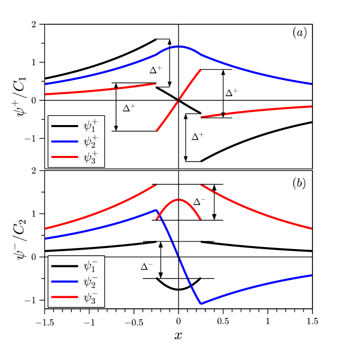
Figure 3: Wave functions $\psi^{\pm}(x)$ for the potential with strengths $V_{11}=V_{22}=V_{33}\equiv V=3\,m$ and $l=0.5\,m^{-1}$ plotted according to formulas (88)–(94). For this potential, the solutions to equations (83) are $E^{+}=0.56\,m$ and $E^{-}=-0.65\,m$. Space $x$ is measured in units of $m^{-1}$.

Notice that the discontinuity of the components $\psi_{1}(x)$ and $\psi_{3}(x)$ at the boundaries $x=x_{1}$ and $x=x_{2}$ is calculated as follows

$$\!\!\!\!\!\!\!\!\!\!\!\!\!\begin{array}[]{ll}\vskip 3.0pt plus 1.0pt minus 1.0pt\psi^{+}_{j}(x_{1}-0)-\psi^{+}_{j}(x_{1}+0)=\psi^{+}_{j}(x_{2}-0)-\psi^{+}_{j}(x_{2}+0)=C_{1}\Delta^{+},\\ \psi^{-}_{j}(x_{1}-0)-\psi^{-}_{j}(x_{1}+0)=\psi^{-}_{j}(x_{2}+0)-\psi^{-}_{j}(x_{2}-0)=C_{2}\Delta^{-},\end{array}$$ (95)

where $j=1,\,3$ and

$$\!\!\!\!\!\!\!\!\!\!\!\!\!\!\!\!\!\!\!\!\!\!\!\!\!\!\!\!\!\Delta^{\pm}={\mu\over\kappa\cos(ka)}\left\{\begin{array}[]{ll}\vskip 3.0pt plus 1.0pt minus 1.0pt\cos(kl/2)&\mbox{for}~{}E=E^{+},\\ \sin(kl/2)&\mbox{for}~{}E=E^{-},\end{array}\right.\;\;\mu:=m-{E\,(V_{1}-V_{3})\over 2E-V_{1}-V_{3}}\,.$$ (96)

In the particular case with $V_{11}=V_{33}\equiv 0$ and an arbitrary $V_{22}$, we have $\mu=0$ for any energy $E$, so that $\psi_{1}(x)$ and $\psi_{3}(x)$ are continuous at $x_{1}$ and $x_{2}$ in this particular case.

4 Characteristic spectra of bound states

Based on equations (83), where $k$ and $\gamma$ are given by expressions (15) and (75), a whole variety of bound states can be materialized, regarding various values of the rectangular potential strengths in formula (15), where $k$ may be either real or imaginary. In particular, on the flat bands defined by equations (17) and (19), expression (15) is simplified, reducing to the equations

$$k=\left\{\begin{array}[]{lll}\vskip 3.0pt plus 1.0pt minus 1.0pt\sqrt{(E-V_{1})(E-V_{3})}&~{}~{}(V_{2}=V_{a})&\mbox{for}~{}{\cal A},\\ \vskip 3.0pt plus 1.0pt minus 1.0pt\sqrt{(E-V_{1})(E-V_{2})}&~{}~{}(V_{1}=V_{3})&\mbox{for}~{}{\cal B},\\ |E-V_{2}|&~{}~{}(V_{1}=V_{2}=V_{3})&\mbox{for}~{}{\cal A}\cap{\cal B}.\end{array}\right.$$ (97)

However, the bound states can also exist if the strengths are found beyond the flat band planes ${\cal A}$ and ${\cal B}$. For the following analysis of the existence of bound states, we restrict ourselves to the investigation on two pencils of straight lines in the $(V_{11},\,V_{22},\,V_{33})$-space using a single strength parameter $V$. In general, a pencil of lines is defined as the set of lines passing through a common point (vertex) in the space. We have chosen two such points in the $(V_{11},\,V_{22},\,V_{33})$-space: $(0,\,0\,0)$ and $(-m,\,0,\,m)$. More precisely, we consider the following two pencil representations:

$$V_{11}=\alpha_{1}V,~{}~{}V_{22}=\alpha_{2}V,~{}~{}V_{33}=\alpha_{3}V,$$ (98)

with the vertex at the origin $(0,\,0,\,0)$ and

$$V_{1}=\alpha_{1}V,~{}~{}~{}V_{2}=\alpha_{2}V,~{}~{}~{}V_{3}=\alpha_{3}V,$$ (99)

with the vertex at the shifted point $(-m,\,0,\,m)$. Here, $\alpha_{j}\in{\mathbb{R}}$, $j=1,\,2,\,3$, with certain constraints to be imposed below in each particular case. In the following, we refer to these representations as to the pencils $P_{1}$ and $P_{2}$, respectively. Correspondingly, wave number (15) takes the following forms:

$$\!\!\!\!\!\!\!\!\!\!\!\!\!\!\!\!\!\!\!\!\!\!\!\!\!k=\sqrt{2(E-\alpha_{1}V-m)(E-\alpha_{2}V)(E-\alpha_{3}V+m)\over 2E-(\alpha_{1}+\alpha_{3})V}\quad\mbox{for pencil}~{}P_{1}$$ (100)

and

$$k=\sqrt{2(E-\alpha_{1}V)(E-\alpha_{2}V)(E-\alpha_{3}V)\over 2E-(\alpha_{1}+\alpha_{3})V}\quad\mbox{for pencil}~{}P_{2}\,.$$ (101)

Some of the lines from the pencils $P_{1}$ and $P_{2}$ fall into the flat band planes ${\cal A}$ and ${\cal B}$. For example, the line with $\alpha_{1}=\alpha_{2}=\alpha_{3}$ from the pencil $P_{1}$ corresponds to the potential referred in [18] as the potential of type I and the corresponding line falls into the ${\cal A}$-plane. The other two particular cases of the pencil $P_{1}$ are $\alpha_{1}=\alpha_{3}=0$, $\alpha_{2}\neq 0$ (type II, as referred in [18]) and $\alpha_{1}\neq 0$, $\alpha_{2}=\alpha_{3}=0$ (type III, as defined in [18]). Both these examples correspond to the potentials with strengths found outside the flat band planes. The lines with $\alpha_{1}=\alpha_{3}$ ($V_{1}=V_{3}$) from the pencil $P_{2}$ fall into the ${\cal B}$-plane. Finally, the particular example $\alpha_{1}=\alpha_{2}=\alpha_{3}$ ($V_{1}=V_{2}=V_{3}$) in the pencil $P_{2}$ corresponds to the ${\cal A}\cap{\cal B}$-line.

Solving equations (83) with $\gamma$ and $k$ given by (75), (100) and (101), for admissible fixed values of the coefficients $\alpha_{j}$’s, one can investigate a bound state energy $E=E_{b}$ (if any) as a function of the strength $V$ on the whole $V$-axis. As demonstrated below, different scenarios of such a behavior occur that depend on the configuration of $\alpha_{j}$’s in the pencils $P_{1}$ and $P_{2}$. Thus, the number of bound states at a given value of $V$ may be finite or even infinite. For some configurations of the coefficients $\alpha_{j}$’s, the number of bound states may increase owing to detachments from the thresholds $E=\pm m$. Notice that, due to equations (72) where $\kappa>0$, for any configuration of potential strengths, the energy $E_{b}$ must be found in the gap $(-m,m)$.

4.1 Bound states with asymptotically periodic energy behavior

Here we introduce the notion ‘asymptotic periodicity’, which means that the solutions to equations (83), consisting of repeating pieces on the $V$-axis, in the limit as $|V|\to\infty$, become exactly periodic. Such a behavior can occur if $\gamma\to$ const.$\,\neq 0$ and $k\propto|V|$ for large $V$. This happens if all the coefficients $\alpha_{j}$’s in both representations (98) and (99) are non-zero. Without loss of generality, one can put here $\alpha_{2}=1$.

For large $V$, the asymptotic representation of equations (83) can be treated as follows. For both the pencils $P_{1}$ and $P_{2}$, according to (75), (100) and (101), we have $k\sim\sqrt{\beta}\,|V|$ and $\gamma\sim-{\rm sgn}(V)\kappa/\sqrt{\beta}\,E$ where

$$\beta:={2\alpha_{1}\alpha_{3}\over\alpha_{1}+\alpha_{3}}\in{\mathbb{R}}\quad(\alpha_{1}+\alpha_{3}\neq 0),$$ (102)

so that asymptotically equations (83) become

$${\kappa\over\sqrt{\beta}\,E}\sim\left\{\begin{array}[]{ll}\vskip 3.0pt plus 1.0pt minus 1.0pt~{}~{}\cot\!\left(\sqrt{\beta}\,Vl/2\right)&\mbox{for}~{}E=E^{+},\\ -\tan\!\left(\sqrt{\beta}\,Vl/2\right)&\mbox{for}~{}E=E^{-}.\end{array}\right.$$ (103)

From these asymptotic relations, for $\beta>0$, we get the periodic behavior:

$$\!\!\!\!\!\!\!\!\!\!\!\!\!\!\!\!\!\!\!\!\!\left(\begin{array}[]{ll}\vskip 3.0pt plus 1.0pt minus 1.0ptE^{+}_{b}\\ E^{-}_{b}\end{array}\right)\simeq{\rm sgn}\!\left(\!\tan{\sqrt{\beta}\,Vl\over 2}\right)m\left(\begin{array}[]{ll}\vskip 3.0pt plus 1.0pt minus 1.0pt~{}~{}\left[1+\beta\cot^{2}(\sqrt{\beta}\,Vl/2)\right]^{-1/2}\\ -\left[1+\beta\tan^{2}(\sqrt{\beta}\,Vl/2)\right]^{-1/2}\end{array}\right)$$ (104)

that confirms the asymptotic periodicity of the bound state energies $E^{\pm}_{b}$ for both the pencils $P_{1}$ and $P_{2}$. In the particular case $\beta=1$, solutions (104) are simplified reducing to the form

$$\left(\begin{array}[]{ll}\vskip 3.0pt plus 1.0pt minus 1.0ptE^{+}_{b}\\ E^{-}_{b}\end{array}\right)\simeq m\left(\begin{array}[]{ll}\vskip 3.0pt plus 1.0pt minus 1.0pt~{}~{}\,{\rm sgn}\!\left[\cos(Vl/2)\right]\sin(Vl/2)\\ -\,{\rm sgn}\!\left[\sin(Vl/2)\right]\cos(Vl/2)\end{array}\right).$$ (105)

Notice that the lines of $P_{1}$ satisfying the condition $\alpha_{1}+\alpha_{3}=2$ fall into the ${\cal A}$-plane [see equation (17)], while the lines of $P_{2}$ with $\alpha_{1}=\alpha_{3}$ appear in the ${\cal B}$-plane [see equation (19)]. The other values of $\alpha_{1}$ and $\alpha_{3}$ correspond to the potentials located outside the flat band planes ${\cal A}$ and ${\cal B}$. In the particular case of $P_{1}$ with $\alpha_{1}=\alpha_{3}=1$ (the potential of type I), we have $\beta=1$ and, as a result, equations (83) reduce to

$$\!\!\!\!\!\!\!\!\!\!\!\!\!\!\!\!\!\!\!\!\!\!\!\!\!{\kappa\over k}\left(1-{V\over E}\right)=\left\{\begin{array}[]{ll}\vskip 3.0pt plus 1.0pt minus 1.0pt-\cot(kl/2)&\mbox{for}~{}E=E^{+},\\ ~{}~{}\tan(kl/2)&\mbox{for}~{}E=E^{-},\end{array}\right.\quad k=\sqrt{(E-V)^{2}-m^{2}}\,.$$ (106)

As follows from the form of these equations, their solutions exist on the whole $V$-axis, where $k$ is real (in the region $|E-V|>m$) and imaginary (in the region $|E-V|<m$), including the lines $|E-V|=m$. For fixed $l$, these solutions are depicted in figure 4.

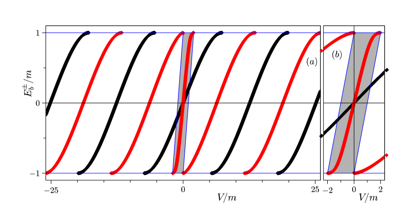
Figure 4: Bound state energies $E_{b}^{+}$ (black lines) and $E_{b}^{-}$ (red lines) as functions of strength $V\in{\mathbb{R}}$ for the line from pencil $P_{1}$ with $\alpha_{1}=\alpha_{2}=\alpha_{3}=1$, $l=0.5\,m^{-1}$. Right panel: Energies in region $|E-V|<m$. In shadowed area, $k$ is imaginary.

In the region $|E-V|<m$ ($k$ is imaginary), one of the solutions (for $E^{+}_{b}$) connects (on both the lines $|E-V|=m$) the pieces of the solution with $k>0$, while the other solution for $E^{-}_{b}$ (completely located in the region $|E-V|<m$) appears as an additional branch in the almost periodic series of the solutions displayed on the whole $V$-axis.

4.2 Spectra with an asymptotically double bound states

In the previous subsection, we have established that the sufficient condition for the periodicity of the bound state spectrum in the limit as $|V|\to\infty$ is $\beta>0$, where $\beta$ is given by relation (102) and the coefficient $\alpha_{2}$ in both the pencils $P_{1}$ and $P_{2}$ is non-zero ($\alpha_{2}=1$). Let us assume now that the parameter $\beta$ is negative. Then, setting ${\rm i}\sqrt{-\beta}$ in asymptotic equations (103) instead of $\sqrt{\beta}$, we arrive at the following two monotonic solutions for large $V$:

$$\!\!\!\!\!\!\!\!\!\!\!\!\!\!\!\!\!\!\!\!\!\!\!\!\!\!\!\!\!\!\!\!\!\!\!\!\!\!\!\!\!\!\left(\begin{array}[]{ll}\vskip 3.0pt plus 1.0pt minus 1.0ptE^{+}_{b}\\ E^{-}_{b}\end{array}\right)\simeq{\rm sgn}(V)\,m\left(\begin{array}[]{ll}\vskip 3.0pt plus 1.0pt minus 1.0pt\left[1-\beta\coth^{2}(\sqrt{-\beta}\,Vl/2)\right]^{-1/2}\\ \left[1-\beta\tanh^{2}(\sqrt{-\beta}\,Vl/2)\right]^{-1/2}\end{array}\right)\!\to{\rm sgn}(V){m\over\sqrt{1-\beta}}\,.$$ (107)

In the particular case of the pencil $P_{2}$ with $\alpha_{1}=\alpha_{3}=-1$ ($\beta=-1$) and $\alpha_{2}=1$, according to (101), we have $k=\sqrt{E^{2}-V^{2}}$, so that the explicit form of equations (83) in the cone region $|E|>|V|$ (where $k$ is real) becomes

$$\!\!\!\!\!\!\!\!\!\!\!\!\!\!\!\!\!{\rm sgn}(E-V){\kappa\over E}\sqrt{E-V\over E+V}=\left\{\begin{array}[]{ll}\vskip 3.0pt plus 1.0pt minus 1.0pt-\cot\!\left(\sqrt{E^{2}-V^{2}}\,l/2\right)&\mbox{for}~{}~{}E=E^{+},\\ ~{}~{}\,\tan\!\left(\sqrt{E^{2}-V^{2}}\,l/2\right)&\mbox{for}~{}~{}E=E^{-}.\end{array}\right.$$ (108)

Beyond the cone, $k$ is imaginary and instead of equations (108), we have

$$\!\!\!\!\!\!\!\!\!\!\!\!\!\!\!\!\!{\rm sgn}(V-E){\kappa\over E}\sqrt{V-E\over V+E}=\left\{\begin{array}[]{ll}\vskip 3.0pt plus 1.0pt minus 1.0pt-\coth\!\left(\sqrt{V^{2}-E^{2}}\,l/2\right)&\mbox{for}~{}~{}E=E^{+},\\ ~{}~{}\,\tanh\!\left(\sqrt{V^{2}-E^{2}}\,l/2\right)&\mbox{for}~{}~{}E=E^{-}.\end{array}\right.$$ (109)

The cone boundary $|E|=|V|$ separates the regions with $k$ real and imaginary ($k=0$) and on this set there are two simple solutions of this equation for $V\in(-m,m)$: $E_{b}^{\pm}=\mp V$. The solutions of equations (108) and (109) are depicted in figure 5. One can specify the $E^{-}_{b}$ solution as a ground state and the $E^{+}_{b}$ solution as an excited state for $V<0$, while for $V>0$ their roles are reversed.

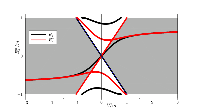
Figure 5: Bound state energies $E_{b}^{\pm}$ as functions of strength $V\in{\mathbb{R}}$ for the line from pencil $P_{2}$ with $\alpha_{1}=\alpha_{3}=-1$ and $\alpha_{2}=1$, $l=5\,m^{-1}$. In shadowed area, $k$ is imaginary.

4.3 Spectra consisting of an infinite number of bound states

Consider now the pencils $P_{1}$ and $P_{2}$, in which $\alpha_{1}+\alpha_{3}=0$ and $\alpha_{2}=1$. Then, setting in this subsection $\alpha_{1}\equiv\alpha=-\alpha_{3}$, for the pencil $P_{1}$, expressions (75) and (100) become

$$\gamma={\kappa\over k}\left(1-{V\over E}\right),\quad k=\sqrt{\left[E^{2}-(\alpha V+m)^{2}\right]\left(1-{V\over E}\right)}\,.$$ (110)

For the pencil $P_{2}$, in this expression for $k$, it is sufficient to set formally $m=0$.

Assume first that $\alpha\neq 0$. Then, using for large $V$ expressions (110), one can represent asymptotically equations (83) in the form

$${\kappa V\over kE}\sim\left\{\begin{array}[]{ll}\vskip 3.0pt plus 1.0pt minus 1.0pt~{}~{}\,\cot(kl/2)&\mbox{for}~{}E=E^{+},\\ -\tan(kl/2)&\mbox{for}~{}E=E^{-},\end{array}\right.\quad k\sim|\alpha|\sqrt{V^{3}\over E}\,.$$ (111)

Since $V/k\to 0$ as $|V|\to\infty$, and taking into account that $|E|<m$, from the right-hand sides of equations (111), we obtain the following approximate solutions for the bound state energies for large $V$:

$$E_{b}^{\pm}=E_{n}\simeq\left({\alpha l\over n\pi}\right)^{\!\!2}\!V^{3},\quad|V|<\left({n\pi\over\alpha l}\right)^{\!2/3}m^{1/3},\quad n=1,\,2,\ldots,$$ (112)

where odd $n$’s stand for $E^{+}_{b}$ and even $n$’s for $E^{-}_{b}$. Here, with increasing the $n$th level, the energies $E_{n}$ are successively cutting at the thresholds $E=\pm m$.

For the illustration of the behavior of the bound state energies on the whole $V$-axis, let us consider the line in the pencil $P_{2}$, for which $\alpha_{1}=\alpha_{2}=-\alpha_{3}=1$. Then, equations (83) take the explicit form as follows

$${\rm sgn}\!\left(1-{V\over E}\right){\kappa\over\sqrt{E(E+V)}}=\left\{\begin{array}[]{ll}\vskip 3.0pt plus 1.0pt minus 1.0pt-\cot(kl/2)&\mbox{for}~{}~{}E=E^{+},\\ ~{}~{}\,\tan(kl/2)&\mbox{for}~{}~{}E=E^{-},\end{array}\right.$$ (113)

with $k=\sqrt{(E^{2}-V^{2})(1-V/E)}$ [instead of $k$ in (110)]. The series of exact solutions of equations (113) is depicted in figure 6, one of which is simple: $E^{+}_{b}=-V$. In this figure, the region where $k$ is real consists of the cone $|E|>|V|$ plus the two strips ($0<E<m$, $0<V<\infty$, $E<V$) and ($-m<E<0$, $-\infty<V<0$, $E>V$). In the region consisting of the two strips ($0<E<m$, $-\infty<V<0$, $E+V<0$) and ($-m<E<0$, $0<V<\infty$, $E+V>0$), $k$ is imaginary. Setting $k={\rm i}\sqrt{(V^{2}-E^{2})(1-V/E)}$ into equations (113) and taking into account that $1-V/E>0$ in these strips, we conclude that the left- and right-hand sides of equations have opposite signs. Therefore there are no solutions in the region where $k$ is imaginary.

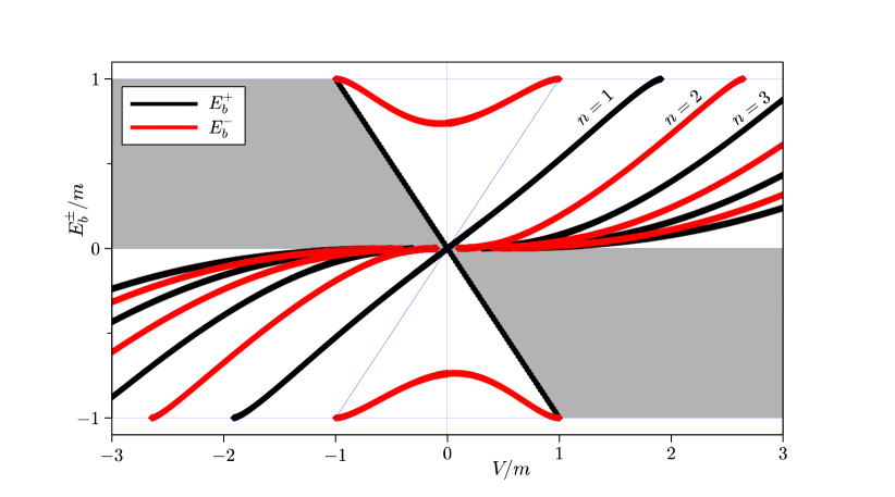
Figure 6: Bound state energies $E_{b}^{\pm}$ as functions of strength $V\in{\mathbb{R}}$ for the line from pencil $P_{2}$ with $\alpha_{1}=\alpha_{2}=-\alpha_{3}=1$, $l=2\,m^{-1}$. In shadowed area, $k$ is imaginary.

Since at the thresholds $E=\pm m$, we have $\kappa=0$, the cutoff of the bound state energies $E_{b}$ is determined by the solutions of the equations $\cot(kl/2)=0$ and $\tan(kl/2)=0$ or correspondingly by the explicit equations $(V+m)^{2}(1-V/m)=(n\pi/l)^{2}$ for $V\leq-m$ and $(V-m)^{2}(1+V/m)=(n\pi/l)^{2}$ for $V\geq m$.

A similar spectrum consisting of an infinite number of bound state energies, but without cutoffs at the thresholds $E=\pm m$, takes also place in the particular case $\alpha=0$, where we are dealing with the potential of type II ($V_{11}=V_{33}=0$, $V_{22}=V$), studied in [18]. More precisely, this is the line from the pencil $P_{1}$ with $\alpha_{1}=\alpha_{3}=0$ and $\alpha_{2}=1$, which does not belong to either the ${\cal A}$- or ${\cal B}$-planes. Thus, owing to (15) and (75), we have

$$k=\kappa\sqrt{{V\over E}-1}\,,\quad\gamma=-\sqrt{{V\over E}-1}\,,$$ (114)

so that equations (83) can be rewritten in the explicit form as follows

$$\sqrt{{V\over E}-1}=\left\{\begin{array}[]{ll}\vskip 3.0pt plus 1.0pt minus 1.0pt~{}~{}\,\cot\!\left[(\kappa l/2)\sqrt{V/E-1}\,\right]&\mbox{for}~{}~{}E=E^{+},\\ -\tan\!\left[(\kappa l/2)\sqrt{V/E-1}\,\right]&\mbox{for}~{}~{}E=E^{-}.\end{array}\right.$$ (115)

Here, $k$ is real in the two strips: ($0<E<m$, $0<V<\infty$ and $E<V$) and ($-m<E<0$, $-\infty<V<0$ and $E>V$). In the case if $k$ is imaginary, the left- and right-hand sides of equations (115) have opposite signs, therefore there are no solutions with imaginary $k$. The solution $E^{-}=V$ that corresponds to $k=0$, splits the regions of real and imaginary $k$’s. This means that the sign of the bound state energy $E_{b}^{+}$ must coincide with the sign of the strength $V$, i.e., the bound state energies $E_{b}^{\pm}$ must be both positive if $V>0$, and negative if $V<0$. The solution of equations (115) on the whole $V$-axis is depicted in figure 7, where it is shown that the $E_{b}^{+}$- and $E_{b}^{-}$-levels alternate. Here, as follows from the form of equations (115), for each $V$, there exists an infinite number of energy levels.

For large $V$, the approximate solution of equations (115), which coincides with formula (33) in [18], reads

$$\!\!\!\!\!\!\!\!\!\!\!\!\!\!\!\!E_{b}^{\pm}=E_{n}\simeq{\rm sgn}(V)\sqrt{{(n\pi/l)^{4}\over 4V^{2}}+m^{2}}-{(n\pi/l)^{2}\over 2V}<m,\quad n=1,\,2\,\ldots,$$ (116)

where even $n$’s stand for $E_{b}^{+}$ and odd $n$’s for $E_{b}^{-}$. There is also a solution that corresponds to $n=0$:

$$E_{b}^{+}=E_{0}\simeq{\rm sgn}(V)\frac{m}{\sqrt{1+(2/Vl)^{2}}},$$ (117)

which faster approaches the threshold values $E=\pm m$ as $|V|\to\infty$. If $V\to 0$, the energy of all the levels is proportional to the potential strength ($E_{n}\propto V)$.

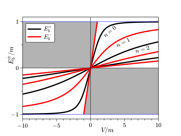
Figure 7: Bound state energies $E_{b}^{\pm}$ as functions of strength $V\in{\mathbb{R}}$ for the line from pencil $P_{1}$ with $\alpha_{1}=\alpha_{3}=0$ and $\alpha_{2}=1$, $l=2\,m^{-1}$. In shadowed area, $k$ is imaginary.

4.4 Bound states with a successive detachment from the thresholds

In this subsection, we describe the spectrum of bound states, the number of which is finite for each fixed strength $V$, however, this number increases with growth of $V$ because of a successive detachment of new bound states from the thresholds $E=\pm m$. To this end, let us consider both the pencils $P_{1}$ and $P_{2}$ with $\alpha_{2}=0$. Notice that the lines with $\alpha_{1}=-\alpha_{3}$ in the pencil $P_{1}$ fall into the ${\cal A}$-plane ($V_{11}+V_{33}=2V_{22}=0$), while the lines with $\alpha_{1}=\alpha_{3}$ in the pencil $P_{2}$ appear in the ${\cal B}$-plane ($V_{1}=V_{3})$.

In general, if $\alpha_{2}=0$, but $\alpha_{1}\neq 0$ and $\alpha_{3}\neq 0$, equations (83) for both the pencils $P_{1}$ and $P_{2}$ can be solved exactly on the whole $V$-axis. The solutions exist only if $k>0$ because for imaginary $k$, both the sides of equations (83) have opposite signs, including the limit $k\to 0$.

Analytically, one can investigate the asymptotic behavior of the bound state spectrum if $V$ is sufficiently large. Thus, for both the pencils $P_{1}$ and $P_{2}$, we have $k\sim\sqrt{-\beta EV}$ with $\beta$ given by (102), so that asymptotically for large $V$, equations (83) become

$$\!\!\!\!\!\!\!\!\!\!\!\!\!\!\!\!\!\!\!\!\!\!{\kappa\over\sqrt{-\beta EV}}\sim\left\{\begin{array}[]{ll}\vskip 3.0pt plus 1.0pt minus 1.0pt-\cot\!\left(\sqrt{-\beta EV}\,l/2\right)&\mbox{for}~{}~{}E=E^{+}\,,\\ ~{}\,\,\tan\!\left(\sqrt{-\beta EV}\,l/2\right)&\mbox{for}~{}~{}E=E^{-}\,.\end{array}\right.$$ (118)

Solving these asymptotic equations and using that $|E|<m$, we get

$$\!\!\!\!\!\!\!\!\!\!\!\!\!\!\!\!\!\!\!\!E_{b}^{\pm}=E_{n}\simeq-{(n\pi/l)^{2}\over\beta V}\,,\quad{(n\pi/l)^{2}\over|\beta|m}<|V|<\infty,\quad n=1,\,2,\ldots,$$ (119)

where odd $n$’s stand for $E^{+}_{b}$ and even $n$’s for $E^{-}_{b}$. One more solution,

$$E_{b}^{-}=E_{0}\simeq-{\rm sgn}(\beta V){m\over\sqrt{1+(\beta Vl/2)^{2}}}$$ (120)

that corresponds to $n=0$, is obtained studying the limit as $EV\to 0$. These solutions are illustrated by figure 8, where an exact solution to equations (83) on the whole $V$-axis is represented for the particular case $\beta=1$. In this case, in equations (83), we have $k=\sqrt{E(E-V)}$ and $\gamma=\kappa/k$.

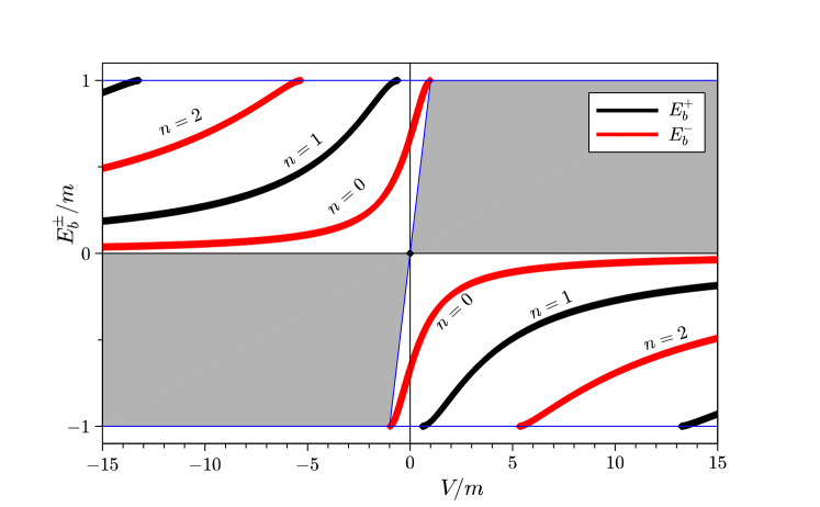
Figure 8: Bound state energies $E_{b}^{\pm}$ as functions of strength $V\in{\mathbb{R}}$ for the line from pencil $P_{1}$ with $\alpha_{1}=\alpha_{3}=1$ and $\alpha_{2}=0$, $l=2.5\,m^{-1}$. In shadowed area, $k$ is imaginary.

One can consider another configuration of the coefficients $\alpha_{j}$ in the pencils $P_{1}$ and $P_{2}$, namely $\alpha_{2}\neq 0$ but $\alpha_{3}=0$. Let us consider the configuration $\alpha_{1}\equiv\alpha>0$, $\alpha_{2}=1$ and $\alpha_{3}=0$ in the pencil $P_{1}$. Then, for large $V$, we have $k\sim\sqrt{-\alpha(m+E)V}$ and therefore equations (83) become

$$\!\!\!\!\!\!\!\!\!\!\!\!\!\!\!\!\!\!\!{\kappa\over E}\sqrt{-{V\over\alpha(m+E)}}\sim\left\{\begin{array}[]{ll}\vskip 3.0pt plus 1.0pt minus 1.0pt-\cot\!\left(\!\sqrt{-\alpha(m+E)V}\,l/2\right)&\mbox{for}~{}~{}E=E^{+}\,,\\ ~{}~{}\,\tan\!\left(\!\sqrt{-\alpha(m+E)V}\,l/2\right)&\mbox{for}~{}~{}E=E^{-}\,.\end{array}\right.$$ (121)

Solving these asymptotic equations for large $V$ and using that $|E|<m$, we get the following approximate solution:

$$\!\!\!\!\!\!\!\!\!\!\!\!\!\!\!\!\!\!\!\!E_{b}^{\pm}=E_{n}\simeq-\left[m+{(n\pi/l)^{2}\over\alpha V}\right],\quad-\infty<V<-{(n\pi/l)^{2}\over 2\alpha m}\,,\quad n=1,\,2,\ldots,$$ (122)

where even $n$’s stand for $E^{+}_{b}$ and odd $n$’s for $E^{-}_{b}$. Except for this solution, there exists also a solution (assigned by the number $n=0$) that approaches the thresholds $E=\pm m$ more rapidly. For $k>0$, only the first equation (121) admits a solution in the limit as $E\to-m$, which must be negative. This solution is valid only for $V<0$ and it coincides with that given by formula (117). On the other hand, for positive $V$, $k$ is imaginary and, as a result, in the limit as $E\to m$ and $V\to\infty$, both equations (121) have also solutions, which coincide in the limit as $V\to\infty$. Thus, on the whole $V$-axis, the $n=0$ bound state energy solution approximately reads

$$E_{b}^{+}=E_{0}\simeq m\left\{\begin{array}[]{ll}\vskip 3.0pt plus 1.0pt minus 1.0pt-\left(1+4/V^{2}l^{2}\right)^{\!-1/2}&\mbox{for}~{}V<0,\\ ~{}~{}\,\left(1+2\alpha m/V\right)^{\!-1/2}&\mbox{for}~{}V>0.\end{array}\right.$$ (123)

Consider the particular case of the line from the pencil $P_{1}$ with $\alpha_{1}=2$, $\alpha_{2}=1$ and $\alpha_{3}=0$. This line falls into the ${\cal A}$-plane and, as follows from representation (100), $k=\sqrt{(m+E)(E-2V-m)}$ , so that equations (83) with this $k$ become

$${\kappa\over k}\left(1-{V\over E}\right)=\left\{\vskip 3.0pt plus 1.0pt minus 1.0pt\begin{array}[]{ll}-\cot(kl/2)&\mbox{for}~{}~{}E=E^{+}\,,\\ ~{}~{}\tan(kl/2)&\mbox{for}~{}~{}E=E^{-}\,.\end{array}\right.$$ (124)

Solving these equations, we obtain the bound state spectrum on the whole $V$-axis, which is depicted in figure 9.

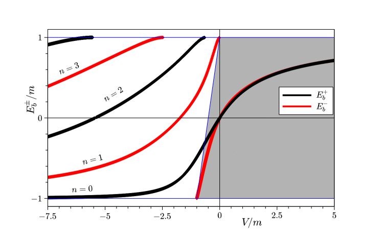
Figure 9: Bound state energies $E_{b}^{\pm}$ as functions of strength $V\in{\mathbb{R}}$ for the line from pencil $P_{1}$ with $\alpha_{1}=2$, $\alpha_{2}=1$ and $\alpha_{3}=0$, $l=2\,m^{-1}$. In shadowed area, $k$ is imaginary.

In the region where $E>2V+m$ and $E\in(-m,m)$, we have $k>0$ and, as a result, along the negative half-axis $V$, the successive detachment of bound state energies occurs. For imaginary $k$, there are two solutions, which are displayed for positive $V$. In the limit as $V\to\infty$, these solutions merge to a single bound state energy.

Thus, we have examined some types of bound state spectra, in which the energy levels $E=E_{b}^{\pm}$ crucially depend on the strength components in the $(V_{11},\,V_{22},\,V_{33})$-space. The set of admissible vectors in this space has been restricted by the two pencils of straight lines $P_{1}$ and $P_{2}$ with the vertices at the points $(0,\,0,\,0)$ and $(-m,\,0,\,m)$. As defined by equations (98) and (99), both the pencils are parametrized by the strength parameter $V$ and the coefficients $\alpha_{j}\in{\mathbb{R}}$, $j=1,\,2,\,3$. Therefore, for a given set of these coefficients, it is possible to describe the bound state energies as functions of the parameter $V$. According to the asymptotic behavior of the energy levels for large values of $V$, from the whole variety of spectra, we have singled out at least four characteristic species, referred in the following to as $P$, $D$, $H$ and $W$ types:

• The spectra of type $P$ are described by the two-valued almost periodic levels $E=E_{b}^{+}$ and $E=E_{b}^{-}$ as illustrated by figure 4. This type is realized on the set

  $$\!\!\!\!\!\!\!\!\!\!\!\!\!\!\!\!\!\!\!\!\!\!\!\!\!\!\!\!A_{P}:=\left\{\alpha_{j}~{}\mbox{in}~{}P_{1}~{}\mbox{and}~{}P_{2}~{}\Big{|}~{}\alpha_{j}\neq 0,\,j=1,\,2,\,3,~{}{\alpha_{1}\alpha_{3}\over\alpha_{1}+\alpha_{3}}>0\right\}.$$ (125)

  The spectra of this type are periodic in the limit as $|V|\to\infty$.

• The spectra of type $D$ are described by the double-valued levels $E=E_{b}^{+}$ and $E=E_{b}^{-}$ with a monotonic behavior for $|V|>m$. In the limit as $|V|\to\infty$, the double levels merge to single levels. This type is materialized on the set

  $$\!\!\!\!\!\!\!\!\!\!\!\!\!\!\!\!\!\!\!\!\!\!\!\!\!\!\!\!A_{D}:=\left\{\alpha_{j}~{}\mbox{in}~{}P_{1}~{}\mbox{and}~{}P_{2}~{}\Big{|}~{}\alpha_{j}\neq 0,\,j=1,\,2,\,3,~{}{\alpha_{1}\alpha_{3}\over\alpha_{1}+\alpha_{3}}<0\right\}$$ (126)

  and illustrated by figure 5.

• The spectra of type $H$, consisting of an infinite number of energy levels that obey the law $E_{b}^{\pm}=E_{n}\propto n^{-2}$, $n\in{\mathbb{N}}$, resemble the hydrogen atom spectrum. One of the spectra of type $H$ includes the levels with successive cutoffs at the thresholds $E=\pm m$ as illustrated by figure 6, so that at a given $V$, the number of levels is finite but it increases to infinity as $|V|\to\infty$. This spectrum is realized on the set

  $$A_{H,1}:=\left\{\alpha_{j}~{}\mbox{in}~{}P_{1}~{}\mbox{and}~{}P_{2}~{}\Big{|}~{}\alpha_{1}=-\alpha_{3}\neq 0,~{}\alpha_{2}\neq 0\right\}.$$ (127)

  The other $H$-spectrum, shown in figure 7, is materialized on the set

  $$A_{H,2}:=\left\{\alpha_{j}~{}\mbox{in}~{}P_{1}~{}\Big{|}~{}\alpha_{1}=\alpha_{3}=0,~{}\alpha_{2}\neq 0\right\}.$$ (128)

  Unlike the previous spectrum, the number of levels is infinite at a given $V$ for this spectrum.

• The spectra of type $W$, consisting of the energy levels $E_{b}^{\pm}=E_{n}\propto n^{2}$, $n\in{\mathbb{N}}$, with their successive detachment from the thresholds $E=\pm m$, resemble the spectrum of a potential well with its increasing depth but fixed width. One of these spectra, illustrated by figure 8, is realized on the set

  $$\!\!\!\!\!\!\!\!\!\!\!\!\!\!\!\!\!\!\!\!\!\!\!\!\!\!\!\!A_{W,1}:=\left\{\alpha_{j}~{}\mbox{in}~{}P_{1}~{}\mbox{and}~{}P_{2}~{}\Big{|}~{}\alpha_{1}\neq 0,~{}\alpha_{3}\neq 0,~{}\alpha_{1}+\alpha_{3}\neq 0,~{}\alpha_{2}=0\right\}.$$ (129)

  The other $W$-spectrum, shown in figure 9, is materialized on the set

  $$A_{W,2}:=\left\{\alpha_{j}~{}\mbox{in}~{}P_{1}~{}\Big{|}~{}\alpha_{1}>0,~{}\alpha_{2}\neq 0,~{}\alpha_{3}=0\right\}.$$ (130)

5 Point interactions realized from rectangular potentials

One-center point interactions can be obtained as the rectangular potentials of type (70) are squeezed to a point. Particularly, based on equations (83), one can materialize one-point interactions with finite bound state energies $E_{b}$ for various types of the potential $V(x)$ in the squeezing limit as $l\to 0$. To accomplish this limit properly, first we have to derive the asymptotic behavior of $k$, $\gamma$ and $\eta$ for small $l$ [according to expressions (15), (75) and (80)] and then to find the $l\to 0$ limit of equations (83) for bound state energies and finally connection matrix (81).

One of these point interactions is the $\delta$-limit of the rectangular potentials

$$\!\!\!\!\!\!\!\!\!\!\!\!\!\!\!\!\!\!\!\!\!V_{jj}(x)={g\over l}\left\{\begin{array}[]{ll}1&\mbox{for}~{}~{}x_{1}\leq x\leq x_{2},\\ 0&\mbox{otherwise}\end{array}\right.\to g\delta(x)\quad\mbox{as}\,\,l\to 0,\,\,~{}~{}~{}g\in{\mathbb{R}},$$ (131)

where $g$ is a dimensionless strength constant of the $\delta$-potential. This a particular case of the regularization of a delta function. More generally, for the approximation of the potential $g\delta(x)$ by regular functions in the one-dimensional Dirac equation, a scaled sequence $l^{-1}h(x/l)$ with $\int_{-\infty}^{\infty}h(\xi)d\xi=g$ has been applied in paper [36]. It should be emphasized that, as proven in this work, the realized point interactions do not depend on the shape of the function $h(\xi)$. In our case, as shown below for some examples of the rectangular potential $V(x)$, the $l^{-1}$-approximation is valid only for ground bound states and it does not ‘cover’ excited states. To describe properly the excited states in a one-point approximation, another type of squeezing is used below, namely with the strength parameter $V\sim g/l^{2}m$ as $l\to 0$. In the following, we refer this type of squeezing to as a ‘$l^{-2}$-limit’. Another type of squeezing to be used is the asymptotic representation $V\sim g(m/l^{2})^{1/3}$, referred to as a ‘$l^{-2/3}$-limit’. Thus, using below the formulas for $k$, $\gamma$ and $\eta$, we will calculate these squeezing limits of equations (83) for several configurations of the potentials $V_{jj}(x)$, $j=1,\,2,\,3$.

We perform the $l\to 0$ limit at the origin of the $(x_{1},\,x_{2})$-plane, setting first $x_{1}\to-0$ and then $x_{2}\to+0$ as one of the ways of approaching the origin. In this case, $a\to 0$ but the repeated limit of the ratio $l/a$ is finite: $\lim_{x_{2}\to+0}\lim_{x_{1}\to-0}(l/a)=2$. Using then the second relation (84), wave functions (93) and (94) are transformed to the form that involves only one arbitrary constant $C_{1}$:

$$\!\!\!\!\!\!\!\!\!\!\!\!\!\begin{array}[]{ll}\vskip 3.0pt plus 1.0pt minus 1.0pt\!\!\!\!\!\!\!\!\!\!\!\!\!\!\!\!\!\!\!\!\!\!\!\!\psi^{+}(x)=C_{1}\left\{\begin{array}[]{ll}\vskip 3.0pt plus 1.0pt minus 1.0pt{\rm col}\!\left(\rho^{-1},\,\sqrt{2}\,,\,\rho\right)\!{\rm e}^{\kappa x},&-\infty<x<0,\\ {\rm col}\!\left(-\rho^{-1},\,\sqrt{2}\,,\,-\rho\right)\!{\rm e}^{-\kappa x},&~{}0<x<\infty,\end{array}\right.~{}~{}\mbox{for}~{}E=E^{+},\\ \!\!\!\!\!\!\!\!\!\!\!\!\!\!\!\!\!\!\!\!\!\!\!\!\psi^{-}(x)=C_{1}\left\{\begin{array}[]{ll}\vskip 3.0pt plus 1.0pt minus 1.0pt{\rm col}\!\left(\rho^{-1},\,\sqrt{2}\,,\,\rho\right)\!{\rm e}^{\kappa x},&-\infty<x<0,\\ {\rm col}\!\left(\rho^{-1},\,-\sqrt{2}\,,\,\rho\right)\!{\rm e}^{-\kappa x},&~{}0<x<\infty,\end{array}\right.~{}~{}~{}~{}\mbox{for}~{}E=E^{-}.\end{array}$$ (132)

Here, $E=E_{b}^{\pm}$ are the $l\to 0$ limit values of the solutions to equations (83). Explicitly, using that $\rho=(m-E)/\kappa$ and $\rho^{-1}=(m+E)/\kappa$, the two-sided (at $x=\pm 0$) boundary conditions for bound states can be represented in the following form:

$$\begin{array}[]{ll}\vskip 3.0pt plus 1.0pt minus 1.0pt\psi^{+}(\pm 0)=C_{1}{\rm col}\left(\mp(m+E^{+}_{b})/\kappa^{+}_{b},\,\sqrt{2},\,\mp(m-E^{+}_{b})/\kappa^{+}_{b}\right),\\ \psi^{-}(\pm 0)=C_{1}{\rm col}\left((m+E^{-}_{b})/\kappa^{-}_{b},\,\mp\sqrt{2},\,(m-E^{-}_{b})/\kappa^{-}_{b}\right),\end{array}$$ (133)

where $\kappa^{\pm}_{b}:=\kappa(E_{b}^{\pm})$. Then $\Lambda$-matrix (81) connects the squeezed boundary conditions of the components $(\psi^{\pm}_{1}-\psi^{\pm}_{3})(x)$ and $\psi^{\pm}_{2}(x)$:

$$\!\!\!\!\!\!\!\!\!\!\!\!\!\!\!\!\!\!\!\!\!\!\!\!\!\!\!\!\!\!\!\!\!\!\!\!\!\!\!\!\!\!\!\!\left(\!\!\!\begin{array}[]{cc}\vskip 3.0pt plus 1.0pt minus 1.0pt(\psi_{1}^{+}-\psi_{3}^{+})(\pm 0)\\ \psi_{2}^{+}(\pm 0)\end{array}\!\!\right)=C_{1}\left(\!\!\begin{array}[]{ll}\vskip 3.0pt plus 1.0pt minus 1.0pt\mp 2E^{+}_{b}/\kappa^{+}_{b}\\ ~{}~{}~{}\sqrt{2}\end{array}\!\!\!\right),~{}\left(\!\!\!\begin{array}[]{cc}\vskip 3.0pt plus 1.0pt minus 1.0pt(\psi_{1}^{-}-\psi_{3}^{-})(\pm 0)\\ \psi_{2}^{-}(\pm 0)\end{array}\!\!\right)=C_{1}\left(\!\!\begin{array}[]{ll}\vskip 3.0pt plus 1.0pt minus 1.0pt2E^{-}_{b}/\kappa^{-}_{b}\\ \,\mp\sqrt{2}\end{array}\!\!\!\right).~{}~{}$$ (134)

Finally, we note that an infinite number of bound states also exists for the potential of type III ($V_{11}=V\in{\mathbb{R}}\setminus\{0\}$ and $V_{22}=V_{33}\equiv 0$), as proven in [18]. However, in the limit as $l\to 0$, for $k$ [see relation (15)] and $\gamma$ we have the limits: $k\to\sqrt{2E(m+E)}$ and $\gamma\to\sqrt{(m-E)/2E}$. Since both these expressions are finite and $kl\to 0$, equations (83) have no solutions, i.e., there are no bound states for the potential of type III in the squeezing limit.

5.1 The $\delta$-limit

Type $P$: The $\delta$-limit of the bound states of type $P$ is obtained immediately by replacing the product $Vl$ in solutions (104) and (105) with the strength $g$. In formula (105), the solution can be combined in the form of the two-valued periodic (increasing) discontinuous function $E=m{\cal E}(g)$, where ${\cal E}(g)$ is constructed from the piece

$$\varepsilon(g)=\left(\begin{array}[]{ll}\varepsilon^{+}(g)\\ \varepsilon^{-}(g)\end{array}\right):=\left(\begin{array}[]{ll}~{}~{}\sin(g/2)&\mbox{for}~{}~{}0\leq g<\pi\\ -\cos(g/2)&\mbox{for}~{}~{}0<g\leq\pi\end{array}\right)$$ (135)

that repeats itself forward and backward along the $g$-axis. The period of the function ${\cal E}(g)$ is $\pi$, so that ${\cal E}(g+\pi)={\cal E}(g)$, $g\in{\mathbb{R}}$. Furthermore, since $kl\to\sqrt{\beta}|g|$ and $\eta\to-{\rm sgn}(g)\sqrt{2/\beta}$ [see equation (80)], in the limit as $l\to 0$, $\Lambda$-matrix (81) reduces to the form

$$\Lambda=\left(\begin{array}[]{lc}\vskip 3.0pt plus 1.0pt minus 1.0pt~{}~{}\cos\!\left(\sqrt{\beta}g\right)~{}~{}~{}~{}~{}~{}-\!\sqrt{2/\beta}\sin\!\left(\sqrt{\beta}g\right)\\ \!\!\sqrt{\beta/2}\sin\!\left(\sqrt{\beta}g\right)~{}~{}~{}~{}~{}~{}~{}\cos\!\left(\sqrt{\beta}g\right)\end{array}\right)$$ (136)

where $\beta>0$. Using expressions (104) for the squeezed energies $E_{b}^{\pm}$, one can check that matrix (136) connects the two-sided boundary values of components (134) at $x=\pm 0$.

Type $D$: Similarly, replacing ${\rm sgn}(V)$ and $Vl$ in bound state energy (107) with ${\rm sgn}(g)$ and $g$, respectively, we obtain the $\delta$-limit of the squeezed energies $E_{b}^{\pm}$. In this case, the connection matrix is described by the same formula (136) where $\beta<0$. In a similar way, using equations (107), one can check that the boundary values (134) are connected by matrix (136) with $\beta<0$.

Type $H$: For realizing a point interaction that corresponds to the ground state, we use the $\delta$-limit defined by (131), setting $V\sim g/l$ in equations (113). Hence, we have $\sqrt{V/E-1}\sim\sqrt{g/E\,l}$ and only the first of equations (115) admits a finite solution in the limit as $l\to 0$. Explicitly, this equation reduces to $\kappa^{+}_{b}/E^{+}_{b}=2/g$, having the solution for the bound state energy:

$$E^{+}_{b}=E_{0}={mg\over\sqrt{4+g^{2}}}$$ (137)

that coincides exactly with formula (13) in [18].

Furthermore, in the limit as $l\to 0$, we have $kl\to 0$ and, according to definition (80), $\eta\sin(kl)\to-\sqrt{2}\,g$. Therefore, matrix (81), connecting the two-sided boundary conditions (134) for the ground state energy $E_{0}$ , becomes

$$\!\!\!\!\!\!\!\!\!\!\!\!\!\!\!\!\Lambda=\Lambda_{0}=\left(\begin{array}[]{lc}1~{}~{}~{}~{}-\sqrt{2}\,g\\ 0~{}~{}~{}~{}~{}~{}~{}~{}~{}1\end{array}\right)=\left(\begin{array}[]{lc}1~{}~{}~{}~{}-2\sqrt{2}\,E_{0}/\sqrt{m^{2}-E_{0}^{2}}\\ 0~{}~{}~{}~{}~{}~{}~{}~{}~{}~{}~{}~{}~{}1\end{array}\right).$$ (138)

Type $W$: Consider the realization of the $\delta$-limit for the pencils $P_{1}$ and $P_{2}$ with $\alpha_{1}\neq 0$, $\alpha_{2}=0$ and $\alpha_{3}\neq 0$. Setting $V\sim g/l$ in expressions (100) and (101), we find that $k\sim\sqrt{-\beta gE/l}$ where $\beta gE<0$. Using this asymptotic representation in equations (118), one can see that only the equation for $E^{-}$ admits a solution in the $l\to 0$ limit. Indeed, in this limit, the second equation (118) reduces to $\kappa/E^{-}=-\beta g/2$, resulting to the ground state energy

$$E^{-}_{b}=E_{0}=-{\rm sgn}(\beta g){m\over\sqrt{1+\beta^{2}g^{2}/4}}\,.$$ (139)

Furthermore, $\eta=\sqrt{2}\,E/k\sim\sqrt{2}\,E/\sqrt{-\beta gE/l}$ and therefore $\eta\sin(kl)\to 0$, while $-\eta^{-1}\sin(kl)\to\beta g/\sqrt{2}$ . Thus, the connection matrix becomes

$$\!\!\!\!\!\!\!\!\!\!\!\!\!\!\!\!\Lambda=\Lambda_{0}=\left(\begin{array}[]{cc}~{}~{}~{}1~{}~{}~{}~{}~{}~{}~{}~{}~{}\,0\\ \beta g/\sqrt{2}~{}~{}~{}~{}~{}1\end{array}\right)=\left(\begin{array}[]{cc}~{}~{}~{}~{}~{}~{}~{}~{}~{}1~{}~{}~{}~{}~{}~{}~{}~{}~{}~{}~{}~{}~{}~{}~{}~{}~{}~{}~{}~{}\,0\\ -\sqrt{2(m^{2}-E_{0}^{2})}/E_{0}~{}~{}~{}~{}~{}1\end{array}\right).$$ (140)

For the other configuration with $\alpha_{1}\equiv\alpha>0$, $\alpha_{2}=1$ and $\alpha_{3}=0$, using the representation $V\sim g/l$, we get $k\sim\sqrt{-\alpha(m+E)g/l}$ . Using this relation in equations (121), we find that only the first equation for $E^{+}$ admits a finite limit, i.e., $2E^{+}=g\kappa$, which can be solved explicitly. Taking into account that $gE>0$, the solution coincides with expression (137). Furthermore, we have the limit $\eta\sin(kl)\to-\sqrt{2}\,g$, resulting in the same connection matrix (138).

5.2 The $l^{-2/3}$-limit

Type $H$: For realizing the point interactions that describe the series of bound states (112), we use the asymptotic representation $V\sim g(m/l^{2})^{1/3}$ with a dimensionless strength $g\in{\mathbb{R}}\setminus\{0\}$. Then, $E_{n}\to(\alpha/n\pi)^{2}g^{3}m$ defined on the intervals $0<|g|<(n\pi/\alpha)^{2/3}$ and $kl\to|\alpha|\sqrt{g^{3}m/E}=n\pi$, $n=1,\,2,\ldots$, with odd $n$’s for $E^{+}_{b}$ and even $n$’s for $E_{b}^{-}$. Due to these relations as well as equations (111), using that $\sin^{2}(kl/2)=1$ if $E_{n}=E^{+}_{b}$ and $\cos^{2}(kl/2)=1$ if $E_{n}=E^{-}_{b}$, one can use the following representation:

$$\!\!\!\!\!\!\!\!\!\!\!\!\!\!\!\!\!\!\!\!\!\!\!\!\!\sin\!\left(\!|\alpha|\sqrt{g^{3}m\over E}\,\right) = 2\left\{\begin{array}[]{ll}\vskip 3.0pt plus 1.0pt minus 1.0pt\sin^{2}\!\left[(|\alpha|/2)\sqrt{g^{3}m/E}\right]\cot\!\left[(|\alpha|/2)\sqrt{g^{3}m/E}\right]\\ \cos^{2}\!\left[(|\alpha|/2)\sqrt{g^{3}m/E}\right]\tan\!\left[(|\alpha|/2)\sqrt{g^{3}m/E}\right]\end{array}\right.$$ (143)

$$\sim 2(-1)^{n+1}\,{2\kappa V\over kE}\,,$$ (144)

where $V/k\to 0$ as $l\to 0$. On the other hand, $\eta\sim-\sqrt{2}\,V/k$ and, as a result, $\eta\sin(kl)\to 0$ and $-\eta^{-1}\sin(kl)\to(-1)^{n+1}\sqrt{2(m^{2}-E^{2})}/E$ as $l\to 0$. Since $\cos(kl)=(-1)^{n}$, connection matrix (81) becomes

$$\!\!\!\!\!\!\!\!\!\!\!\!\!\!\!\!\!\!\!\!\!\!\!\!\!\!\!\!\!\!\!\!\!\!\!\!\!\!\!\!\!\!\Lambda=\Lambda_{n}=(-1)^{n}\left(\!\!\begin{array}[]{cc}\vskip 3.0pt plus 1.0pt minus 1.0pt~{}~{}~{}~{}~{}~{}~{}~{}~{}~{}~{}1~{}~{}~{}~{}~{}~{}~{}~{}~{}~{}~{}~{}~{}~{}~{}~{}~{}~{}~{}0\\ -\sqrt{2(m^{2}-E^{2}_{n})}/E_{n}~{}~{}~{}~{}~{}~{}1\end{array}\!\!\right),~{}~{}E_{n}=\left({\alpha\over n\pi}\right)^{2}g^{3}m,~{}~{}n\in{\mathbb{N}}.$$ (145)

5.3 The $l^{-2}$-limit

Type $H$: For realizing the point interactions that describe the excited bound states with energies (116), we use the asymptotic representation $V\sim g/l^{2}m$ with a dimensionless strength $g\in{\mathbb{R}}\setminus\{0\}$. Then equations (115) asymptotically become

$$\sqrt{mE\over g}\,l\,\sim\,\left\{\begin{array}[]{ll}\vskip 3.0pt plus 1.0pt minus 1.0pt~{}~{}\,\tan\!\left[(\kappa/2)\sqrt{g/mE}\,\right]&\mbox{for}~{}~{}E=E^{+},\\ -\cot\!\left[(\kappa/2)\sqrt{g/mE}\,\right]&\mbox{for}~{}~{}E=E^{-}.\end{array}\right.$$ (146)

In the limit as $l\to 0$, both these asymptotic relations lead to the series of equations $kl\to\kappa\sqrt{g/mE}=n\pi$, $n=1,2,\ldots$, where $E=E^{+}_{b}$ stands for even $n$’s and $E=E^{-}_{b}$ for odd $n$’s. The solution of these equations with respect to $E\in(-m,m)$ reads

$$\!\!\!\!\!\!\!\!\!\!\!\!E_{b}^{\pm}=E_{n}={n^{2}\pi^{2}m\over 2g}\left(\sqrt{1+{4g^{2}\over n^{4}\pi^{4}}}-1\right)\simeq{gm\over n^{2}\pi^{2}}\,,~{}~{}~{}n\in{\mathbb{N}},~{}~{}$$ (147)

supporting the $1/n^{2}$ law only for the excited states. Note that $E_{n}\in(0,m)$ if $g>0$ and $E_{n}\in(-m,0)$ if $g<0$.

Furthermore, from (80) we have $\eta\sim-(g/\kappa l)\sqrt{2E/mg}$ . On the other hand, using representation (146), we obtain

$$\sin\!\left(\!\kappa\sqrt{g\over mE}\,\right) = 2\left\{\begin{array}[]{ll}\vskip 3.0pt plus 1.0pt minus 1.0pt\tan\!\left[(\kappa/2)\sqrt{g/mE}\,\right]\cos^{2}\!\left[(\kappa/2)\sqrt{g/mE}\,\right]\\ \sin^{2}\!\left[(\kappa/2)\sqrt{g/mE}\,\right]\cot\!\left[(\kappa/2)\sqrt{g/mE}\,\right]\end{array}\right.$$ (150)

$$\sim 2(-1)^{n}\,\sqrt{mE\over g}\,l,$$ (151)

where even $n$’s correspond to $E^{+}_{b}$ and odd $n$’s to $E^{-}_{b}$. As a result, in the limit as $l\to 0$, we obtain $\eta\sin(kl)\to-2\sqrt{2}\,(-1)^{n}E_{n}/\sqrt{m^{2}-E_{n}^{2}}$. Since $\cos(kl)\to(-1)^{n}$, taking for account matrix (138), the connection matrix for all the bound states reads as follows

$$\!\!\!\!\!\!\!\!\!\!\!\!\!\!\!\!\!\!\!\!\!\!\!\!\!\!\Lambda=\Lambda_{n}=(-1)^{n}\left(\!\!\begin{array}[]{cc}\vskip 3.0pt plus 1.0pt minus 1.0pt1~{}~{}~{}~{}-2\sqrt{2}\,E_{n}/\sqrt{m^{2}-E^{2}_{n}}\\ 0~{}~{}~{}~{}~{}~{}~{}~{}~{}~{}~{}~{}~{}~{}~{}~{}~{}~{}~{}~{}~{}~{}1{}{}{}{}{}{}{}{}{}{}\end{array}\!\!\right),~{}~{}~{}~{}n\in{\mathbb{N}}\cup\{0\},$$ (152)

where $E_{n}=E_{b}^{+}$ for even $n$ and $E_{n}=E_{b}^{-}$ for odd $n$. Here, the ground state energy $E_{0}$ is given by expression (137) and excited state energies by equations (147). These energies are arranged as $m>|E_{0}|>|E_{1}|>\ldots>|E_{n}|>\ldots$ for all $g\in{\mathbb{R}}\setminus\{0\}$. Notice that in matrix (152), for $n=1,2,\ldots$, we have $E_{n}/\sqrt{m^{2}-E_{n}^{2}}\simeq g/n^{2}\pi^{2}$ .

Type $W$: To implement point interactions that describe the excited bound states for the pencils $P_{1}$ and $P_{2}$ with $\alpha_{1},\,\alpha_{3}\neq 0$ and $\alpha_{2}=0$, we substitute the asymptotic representation $V\sim g/l^{2}m$ into equations (118). As a result, these equations become

$${\kappa\over\sqrt{-\beta gE/m}}\,l\,\sim\,\left\{\begin{array}[]{ll}\vskip 3.0pt plus 1.0pt minus 1.0pt-\cot(\sqrt{-\beta gE/m}/2)&\mbox{for}~{}~{}E=E^{+}\,,\\ ~{}~{}\,\tan(\sqrt{-\beta gE/m}/2)&\mbox{for}~{}~{}E=E^{-}\,.\end{array}\right.$$ (153)

In the limit as $l\to 0$, from these equations we obtain the solution

$$E_{b}^{\pm}=E_{n}=-{n^{2}\pi^{2}m\over\beta g}\,,~{}~{}~{}n\in{\mathbb{N}},$$ (154)

where odd $n$’s stand for $E_{b}^{+}$ and even $n$’s for $E_{b}^{-}$. Using further asymptotic representation (153), one can write

$$\sin\sqrt{-\beta gE\over m} = 2\left\{\begin{array}[]{ll}\vskip 3.0pt plus 1.0pt minus 1.0pt\sin^{2}\!\left[\sqrt{-\beta gE/m}/2\right]\cot\!\left[\sqrt{-\beta gE/m}/2\right]\\ \tan\!\left[\sqrt{-\beta gE/m}/2\right]\cos^{2}\!\left[\sqrt{-\beta gE/m}/2\right]\end{array}\right.$$ (157)

$$\sim 2(-1)^{n}\,{\kappa\over\sqrt{-\beta gE/m}}\,l,$$ (158)

where odd $n$’s correspond to $E^{+}_{b}$ and even $n$’s to $E^{-}_{b}$. Therefore, in the limit as $l\to 0$, we have $\eta^{-1}\sin(kl)\to(-1)^{n}\sqrt{2(m^{2}-E_{n}^{2})}\,/E_{n}\,.$ Since $\cos(kl)\to(-1)^{n}$, taking for account matrix (140), the connection matrix for all the bound states reads as follows

$$\!\!\!\!\!\!\!\!\!\!\!\!\!\!\!\!\!\!\!\!\!\!\!\!\!\Lambda=\Lambda_{n}=(-1)^{n}\left(\!\!\begin{array}[]{cc}\vskip 3.0pt plus 1.0pt minus 1.0pt~{}~{}~{}~{}~{}~{}~{}~{}~{}1~{}~{}~{}~{}~{}~{}~{}~{}~{}~{}~{}~{}~{}~{}~{}~{}~{}~{}~{}~{}~{}~{}0\\ -\sqrt{2(m^{2}-E_{n}^{2})}\,/E_{n}~{}~{}~{}~{}~{}~{}~{}1{}\end{array}\!\!\right),~{}~{}~{}~{}n\in{\mathbb{N}}\cup\{0\},$$ (159)

where the bound state energies $E_{n}$ are given by expressions (139) and (154) with $E_{n}=E_{b}^{+}$ for odd $n$ and $E_{n}=E_{b}^{-}$ for even $n$. Here $E_{0}$ is a ground state energy and the energies $E_{n}$ with $n=1,\,2,\ldots$ correspond to excited states. These energies are arranged as $m>|E_{0}|>|E_{1}|>\ldots>|E_{n}|>\ldots$ for all $g\in{\mathbb{R}}\setminus\{0\}$.

Similarly, for the case of the pencil $P_{1}$ with $\alpha_{1}\equiv\alpha>0$, $\alpha_{2}=1$ and $\alpha_{3}=0$, owing to the relation $V\sim g/l^{2}m$, we have $k\sim\sqrt{-\alpha(1+E/m)g}/l$ with $g<0$. Further, the asymptotic representation of equations (121) reads

$$\!\!\!\!\!\!\!\!\!\!\!\!\!{E\sqrt{\alpha m(m+E)}\over\kappa\sqrt{-g}}\,l\,\sim\,\left\{\begin{array}[]{ll}\vskip 3.0pt plus 1.0pt minus 1.0pt-\tan\!\left[\sqrt{-\alpha(1+E/m)g}/2\right]&\mbox{for}~{}~{}E=E^{+}\,,\\ ~{}~{}\,\cot\!\left[\sqrt{-\alpha(1+E/m)g}/2\right]&\mbox{for}~{}~{}E=E^{-}\,.\end{array}\right.$$ (160)

In the limit as $l\to 0$, from these equations, we obtain $\sqrt{-\alpha(1+E/m)g}=n\pi,~{}n=1,\,2,\ldots$, where even $n$’s stand for $E^{+}$ and odd $n$’s for $E^{-}$. Solving the last equation and taking for account that $|E|<m$, we get the series of excited bound states with the energies

$$\!\!\!\!\!\!\!\!\!\!\!\!\!\!\!\!\!\!\!\!\!\!\!\!\!\!E_{b}^{\pm}=E_{n}=-\left(1+{n^{2}\pi^{2}\over\alpha g}\right)\!m,\quad-\infty<g<-{n^{2}\pi^{2}\over 2\alpha}\,,~{}~{}~{}n\in{\mathbb{N}}.$$ (161)

These energies are detached successively from the upper threshold $E=m$. Using relations (137) and (161), one can prove that the bound state energies are arranged in the order $E_{0}<E_{1}<\ldots E_{n}<\ldots$.

Using further asymptotic representation (160), one can write

$$\!\!\!\!\!\!\!\!\!\!\!\!\!\!\!\!\!\!\!\!\!\!\!\!\!\!\!\!\!\!\!\!\sin\!\sqrt{-\alpha(1+E/m)g} = 2\left\{\begin{array}[]{ll}\vskip 3.0pt plus 1.0pt minus 1.0pt\cos^{2}[\sqrt{-\alpha(1+E/m)g}/2]\,\tan[\sqrt{-\alpha(1+E/m)g}/2]\\ \sin^{2}[\sqrt{-\alpha(1+E/m)g}/2]\,\cot[\sqrt{-\alpha(1+E/m)g}/2]\end{array}\right.$$ (164)

$$\sim 2(-1)^{n+1}\,{E\sqrt{\alpha m(m+E)}\over\kappa\sqrt{-g}}\,l,$$ (165)

where even $n$’s correspond to $E^{+}_{b}$ and odd $n$’s to $E^{-}_{b}$. Next, in the limit as $l\to 0$, we have $\eta\sin(kl)\to(-1)^{n+1}2\sqrt{2}\,E_{n}/\sqrt{m^{2}-E_{n}^{2}}$ . Since $\cos(kl)\to\cos\sqrt{-\alpha(1+E/m)g}=(-1)^{n}$, taking for account matrix (138), the connection matrix for all the bound states is the same as for the potential of type II given by matrix (152). Here, the energies $E_{n}$ with $n=1,\,2,\ldots$ correspond to the excited states.

Thus, the equations derived above for the bound state energies in the squeezing limit indicate that only those energy levels, which are stretched on the $V$-axis to infinity, as illustrated by figures from 4 to 9, admit a point approximation. The levels with a finite support, which are shown in figures 4–7 and 9, are not appropriate for implementing point interactions. The energies $E_{b}^{\pm}$ in the squeezing limit become functions of the dimensionless strength constant $g$.

The point interactions considered above are determined by the matrices that connect the two-sided boundary conditions for a wave functions $\psi^{\pm}(x)$ at the origin $x=\pm 0$. To implement these interactions, we have applied three rates of squeezing as $l\to 0$. One of these is the $l^{-1}$-limit resulting in the typical $\delta$-interaction. In this limit, for the spectra of types $P$ and $D$, the connection matrix is given by (136), where $\beta>0$ and $\beta<0$ correspond to perfectly periodic energies (104) and to double-valued energies (107), respectively, with ${\rm sgn}(V)$ and $Vl$ substituted by ${\rm sgn}(g)$ and $g$. For the spectra of types $H$ and $W$, the $l^{-1}$-limit leads to the existence of ground states, which are indicated in table 1 with $n=0$.

The $l^{-2/3}$- and $l^{-2}$-limits generate the countable sets of point interactions that describe the excited states in the $H$- and $W$-spectra. As indicated in table 1, for these interactions, there are two connection matrices

$$\!\!\!\!\!\!\!\!\!\!\!\!\!\!\!\!\!\!\!\!\!\!\!\!\!\!\!\!\!\!\!\!\!\!\!\!\!\!\!\!\!\!\!\Lambda_{n}=\left(\begin{array}[]{cc}~{}1~{}~{}~{}~{}0\\ 2\chi_{n}~{}~{}1\end{array}\right)~{}\mbox{and}~{}\left(\begin{array}[]{cc}1~{}~{}~{}2/\chi_{n}\\ \!\!\!\!0~{}~{}~{}~{}~{}1{}\end{array}\right),~{}~{}\chi_{n}:=-{\sqrt{(m^{2}-E_{n}^{2})/2}\over E_{n}},~{}~{}n\in{\mathbb{N}}\cup\{0\}.~{}~{}~{}$$ (166)

It should be noticed that the $l^{-2}$-limit has been applied in many publications (see, e.g., [31, 32, 33, 34, 35, 37, 38, 39], a few to mention), mainly for regularizing a potential in the form of the derivative of a delta function in the non-relativistic Schrödinger equation.

Table 1: Squeezed connection matrices and bound state energies for point interactions of types $H$ and $W$ obtained in the $l\to 0$ limit with three rates $l^{-1}$, $l^{-2}$ and $l^{-2/3}$. The energy levels, shown in figures 6–9, which admit the realization of the point interactions, are indicated in the last column.

Connection	$A$-sets	Types	Squeezing	Bound state	Energy
matrices $\Lambda_{n}$		of spectra	limits	energies	levels in figures
$(-1)^{n}\left(\!\!\begin{array}[]{cc}~{}1~{}~{}~{}~{}\,0\\ 2\chi_{n}~{}~{}1\end{array}\!\right)$	$A_{H,1}$	$H$	$l^{-2/3}$	$E_{n}$ in (145)	6 ($n\in{\mathbb{N}}$)
	$A_{W,1}$	$W$	$l^{-1}$	$E_{0}$ in (139)	8 ($n=0$)
	$A_{W,1}$	$W$	$l^{-2}$	$E_{n}$ in (154)	8 ($n\in{\mathbb{N}}$)
$(-1)^{n}\left(\!\!\begin{array}[]{cc}1~{}~{}~{}2/\chi_{n}\\ 0~{}~{}~{}~{}~{}1{}{}{}\end{array}\!\!\!\right)$	$A_{H,2}$	$H$	$l^{-1}$	$E_{0}$ in (137)	7 ($n=0$)
	$A_{H,2}$	$H$	$l^{-2}$	$E_{n}$ in (147)	7 ($n\in{\mathbb{N}}$)
	$A_{W,2}$	$W$	$l^{-1}$	$E_{0}$ in (137)	9 ($n=0$)
	$A_{W,2}$	$W$	$l^{-2}$	$E_{n}$ in (161)	9 ($n\in{\mathbb{N}}$)

Finally, knowing the bound state energies in the squeezing limit and therefore the values $\rho(E_{b}^{\pm})$, one can plot the eigenfunctions given by (134). Here, we have restricted ourselves to the bound states of type $P$ (see figure 10) and $H$ (see figure 11).

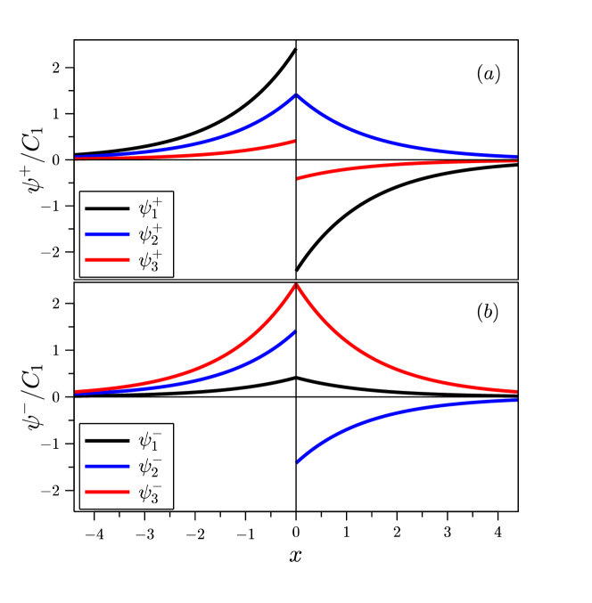
Figure 10: Squeezed eigenfunctions $\psi^{\pm}(x)$ that correspond to spectrum of type $P$, which have been plotted according to formulas (132). Here, the bound state energies $E_{b}^{\pm}$, obtained in the $l^{-1}$-limit, are given by equations (135): (a) $E_{b}^{+}/m=\sin(g/2)$ and (b) $E_{b}^{-}/m=-\cos(g/2)$ with strength $g=\pi/2$.

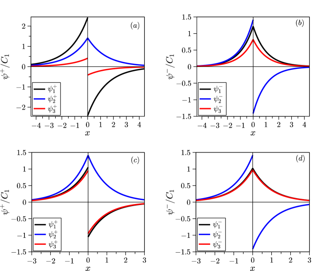
Figure 11: Squeezed eigenfunctions $\psi^{\pm}(x)$ that correspond to spectrum of type $H$, given by equations (132) and implemented on set $A_{H,2}$. Bound state energies $E_{b}^{\pm}=E_{n}$, obtained in the $l^{-2}$-limit, are computed for the four lowest energy levels: (a) $n=0$, (b) $n=1$, (c) $n=2$, (d) $n=3$, in accordance with equations (137) for $E_{0}$ and (147) for $E_{n}$, $n=1,\,2,\,3$, with strength $g=2$.

6 Concluding remarks

The energy spectrum of the ordinary one-dimensional non-relativistic Hamiltonian for a particle in a constant potential field $V(x)\equiv V\in{\mathbb{R}}$ is quite trivial: it is just the shift of a free-particle spectrum by the strength $V$. The spectrum of the one-dimensional pseudospin-one Hamiltonian with a constant three-component potential $V(x)={\rm col}(V_{11},\,V_{22},\,V_{33})$ consists of three (upper, middle and lower) bands, which are described by cubic equation (11). The structure of this spectrum crucially depends on the relative configuration of the strengths $V_{11},\,V_{22}$, $V_{33}$ and all the possible forms of the bands are illustrated by figure 1. In this regard, each strength configuration can be associated with a vector in the three-dimensional space $(V_{11},\,V_{22},\,V_{33})$ and only in the particular case of the line $V_{11}=V_{22}=V_{33}\equiv V$ in this space, free-particle spectrum (4) with eigenfunctions (41) is shifted by $V$, equally in each band, similarly to the situation with a non-relativistic Hamiltonian.

Almost all the points in the $(V_{11},\,V_{22},\,V_{33})$-space correspond to the energy spectrum, in which the middle band is dispersive. At some limiting points in this space, the middle band as a function of the wave number $k$ shrinks to a line, the so-called flat band, as shown in panels (d) and (h)–(j) of figure 1. This set, shown in figure 2, consists of the two intersecting planes ${\cal A}$ and ${\cal B}$, which are defined by equations (17) and (19). The energy of the upper and lower dispersion bands on these planes are described by solutions (22) and (24). The corresponding eigenfunctions are given through the general formula (13).

To implement bound states in the pseudospin-one Hamiltonian, the components of the potential $V(x)$ must be localized on the $x$-axis. To this end, we have chosen these components in the form of rectangles that represent a layer of thickness $l=x_{2}-x_{1}$, where $x=x_{1}$ and $x=x_{2}$ are arbitrary points. Then one can use the general solution (13) for the interval $x_{1}\leq x\leq x_{2}$ complementing it by the free-particle solution beyond this interval that decreases as $|x|\to\infty$ and using the matching conditions at the edges $x_{1}$ and $x_{2}$. Within this approach, a pair of general equations (83) has been derived for finding bound state energies. The solutions to these equations are conditionally denoted as $E^{+}=E_{b}^{+}$ for the first equation (83) and $E^{-}=E_{b}^{-}$ for the second one. The corresponding eigenfunctions $\psi^{+}(x)$ and $\psi^{-}(x)$ are illustrated by expressions (88)–(94) and figure 3.

As demonstrated by figures from 4 to 9, the structure of the bound state spectrum crucially depends on the configuration of the strengths $V_{11}$, $V_{22}$ and $V_{33}$ that determine the rectangular potentials. For simplicity, instead of these three independent strengths as vectors in the ${\mathbb{R}}^{3}$-space, we have restricted ourselves to the investigation on the two pencils of straight lines in ${\mathbb{R}}^{3}$ defined by equations (98) and (99), where only one strength parameter $V$ is incorporated. Even on these particular sets, a whole variety of bound states has been proven to exist. Based on the asymptotic behavior of the solutions to equations (83) in the limit as $|V|\to\infty$, one can single out the four types of bound states, which we call in the present work as $P$, $D$, $H$ and $W$. The energies for two of these types ($P$ and $H$) have already been investigated earlier in paper [18]. In the present work, the study of these energies has been supplemented by the solutions with imaginary wave number $k$. Particularly, for the potentials with all the three strengths $V_{11}$, $V_{22}$ and $V_{33}$ $\propto$ $V$, the energy spectrum of the type $P$ consists of two levels and the dependence on $V$ is almost periodic (and exact periodic in the limit as $|V|\to\infty$). Surprisingly, the energy spectrum of the type $H$ consists of an infinite number of levels, resembling the hydrogen atom spectrum ($E_{n}\propto 1/n^{2}$, $n=1,2,\ldots$). It should be noticed that a successive cutoff of energy levels with the growth of the strength $V$ is possible for the type $H$ (compare figures 6 and 7). In addition to the types $P$ and $H$, we have examined the spectrum that consists of two levels for large $V$ (type $D$) merging into a single level in the limit as $|V|\to\infty$. Another behavior of the bound-state energies, which has been observed in the present work, is a successive detachment of energy levels from the thresholds of upper and lower continuums $E=\pm m$ with increasing the strength $V$ (type $W$). This behavior resembles the energy spectrum of an ordinary potential well as its depth $V$ tends to infinity at fixed width. The energy levels for this type have been shown to behave as $E_{n}\propto n^{2}$, $n=1,2,\ldots$.

For some bound state energy levels, it is possible to use a one-point approximation through the squeezing limit $l\to 0$ and $V\to\infty$. To implement such a procedure explicitly, we consider the strength parameter $V$ as a function of $l$ imposing an appropriate behavior as $l\to 0$. For realizing a well-defined point interaction, it is sufficient to construct a matrix that connects the two-sided values of the wave function given at the point of singularity (for instance, at $x=\pm 0$). To this end, we have derived the general form of such a matrix for arbitrary points $x_{1}$ and $x_{2}$ given by equation (81). Further, in each special case, setting $x_{1}\to-0$ and $x_{2}\to+0$, we have realized the following three families of one-center point interactions using the asymptotic behavior of $V$ as $l\to 0$: (i) $V\sim g/l$ ($\delta$-limit), (ii) $V\sim g(m/l^{2})^{1/3}$ ($l^{-2/3}$-limit) and (iii) $V\sim g/l^{2}m$ ($l^{-2}$-limit), where $g$ is a dimensionless coupling constant.

In conclusion, it would be interesting to develop a more general approach for studying bound states, which avoids the presentation of the three strengths $V_{11}$, $V_{22}$ and $V_{33}$ through one parameter $V$. In this way, it could be possible to obtain additional types of bound state spectra. The investigation of the systems with a long-range Coulomb potential, instead of piecewise potentials, is of big interest as well. The study of the scattering problem in the presence of multiple point potentials, including resonance effects as well as bound states in the continuum, is also of great interest.

Data availability statement

The data that support the findings of this study are available upon reasonable request from the authors.

Acknowledgments

We would like to thank the Armed Forces of Ukraine for providing security to perform this work. A.V.Z. acknowledges financial support from the National Academy of Sciences of Ukraine, Project No. 0123U102283. Y.Z. and V.P.G. acknowledge financial support by the National Research Foundation of Ukraine grant (2020.02/0051) ‘Topological phases of matter and excitations in Dirac materials, Josephson junctions and magnets’. Finally, we are indebted to the anonymous Referees for the careful reading of this paper, their questions and suggestions, resulting in the significant improvement of the paper.

References

References

- [1] Bradlyn B, Cano J, Wang Z, Vergniory M G, Felser C, Cava R J and Bernevig B A 2016 Beyond Dirac and Weyl fermions: Unconventional quasiparticles in conventional crystals Science 353 558
- [2] Bercioux D, Urban D F, Grabert H and Häsler W 2009 Massless Dirac-Weyl fermions in a optical lattice Phys. Rev. A 80 063603
- [3] Raoux A, Morigi M, Fuchs J-N, Piéchon F and Montambaux G 2014 From dia- to paramagnetic orbital susceptibility of massless fermions Phys. Rev. Lett. 112 026402
- [4] Leykam D, Andreanov A and Flach S 2018 Artificial flat band systems: from lattice models to experiments Adv. Phys.: X 3 1473052
- [5] Tasaki H 1998 From Nagaoka’s ferromagnetism to flat-band ferromagnetism and beyond: An introduction to ferromagnetism in the Hubbard model Prog. Theor. Phys. 99 489
- [6] Cao Y, Fatemi V, Fang Ah, Watanabe K, Taniguchi T, Kaxiras E and Jarillo-Herrero P 2018 Unconventional superconductivity in magic-angle graphene superlattices Nature 556 43
- [7] Andrei E Y and MacDonald A H 2020 Graphene bilayers with a twist Nature Materials 19 1265
- [8] Illes E, Carbotte J P and Nicol E J 2015 Hall quantization and optical conductivity evolution with variable Berry phase in the model Phys. Rev. B 92 245410
- [9] Kovacs A D, David G, Dora B and Cserti J 2017 Frequency-dependent magneto-optical conductivity in the generalized model Phys. Rev. B 95 035414
- [10] Iurov A, Zhemchuzhna L, Dahal D, Gumbs G and Huang D 2020 Quantum-statistical theory for laser-tuned transport and optical conductivities of dressed electrons in materials Phys. Rev. B 101 035129
- [11] Biswas T and Ghosh T K 2016 Dynamics of a quasiparticle in the model: role of pseudospin polarization and transverse magnetic field onzitterbewegung J. Phys.: Condens. Mattter 28 495302
- [12] Islam Firoz S K and Dutta P 2017 Valley-polarized magnetoconductivity and particle-hole symmetry breaking in a periodically modulated lattice Phys. Rev. B 96 045418
- [13] Oriekhov D O and Gusynin V P 2020 RKKY interaction in a doped pseudospin-1 fermion system at finite temperature Phys. Rev. B 101 235162
- [14] Roslyak O, Gumbs G, Balassis A and Elsayed H 2021 Effect of magnetic field and chemical potential on the RKKY interaction in the lattice Phys. Rev. B 103 075418
- [15] Gorbar E V, Gusynin V P and Oriekhov D O 2019 Electron states for gapped pseudospin-1 fermions in the field of a charged impurity Phys. Rev. B 99 155124
- [16] Van Pottelberge R 2020 Comment on ‘Electron states for gapped pseudospin-1 fermions in the field of a charged impurity’ Phys. Rev. B 101 197102
- [17] Yi-Cai Zhang 2022 Wave function collapses and energy spectrum induced by a Coulomb potential in a one-dimensional flat band system Chin. Phys. B 31 050311
- [18] Yi-Cai Zhang and Guo-Bao Zhu 2022 Infinite bound states and hydrogen atom-like energy spectrum induced by a flat band J. Phys. B: At. Mol. Opt. Phys. 55, 065001
- [19] Yi-Cai Zhang 2022 Infinite bound states and energy spectrum induced by a Coulomb-like potential of type III in a flat band system Phys. Scr. 97 015401
- [20] Jakubský V and Zelaya K 2023 Lieb lattices and pseudospin-1 dynamics under barrier- and well-like electrostatic interactions Physica E: Low-dimensional Systems and Nanostructures 152 115738
- [21] Jakubský V and Zelaya K 2023 Landau levels and snake states of pseudo-spin-1 Dirac-like electrons in gapped Lieb lattices J. Phys.: Condens. Matter 35 025302
- [22] Pichon F, Fuchs J-N, Raoux A and Montambaux G 2015 Tunable orbital susceptibility in tight-binding models J. Phys.: Conf. Ser. 603 012001
- [23] Demkov Y N and Ostrovskii V N 1975 Zero-Range Potentials and Their Applications in Atomic Physics (Leningrad: Leningrad University Press)
- [24] Demkov Y N and Ostrovskii V N 1988 Zero-Range Potentials and Their Applications in Atomic Physics (New York: Plenum)
- [25] Albeverio S, Gesztesy F, Høegh-Krohn R and Holden H 2005 Solvable Models in Quantum Mechanics (With an Appendix by Pavel Exner) 2nd revised edn (Providence: RI: American Mathematical Society: Chelsea Publishing)
- [26] Albeverio S and Kurasov P 1999 Singular Perturbations of Differential Operators: Solvable Schrödinger-Type Operators (Cambridge: Cambridge University Press)
- [27] Zolotaryuk A V and Zolotaryuk Y 2011 Controlling a resonant transmission across the -potential: the inverse problem J. Phys. A: Math. Theor. 44 375305; 2012 Corrigendum: Controlling a resonant transmission across the -potential: the inverse problem J. Phys. A: Math. Theor. 45 119501
- [28] Zolotaryuk A V and Zolotaryuk Y 2015 A zero-thickness limit of multilayer structures: a resonant-tunnelling -potential J. Phys. A: Math. Theor. 48 035302
- [29] Gusynin V P, Sobol O O, Zolotaryuk A V and Zolotaryuk Y 2022 Bound states of a one-dimensional Dirac equation with multiple delta-potentials Low Temp. Phys. 48 1022
- [30] Ibarra-Reyes M, Prez-lvarez R and Rodríguez-Vargas I 2023 Transfer matrix in 1D Dirac-like problems J. Phys.: Condens. Mattter 35 395301
- [31] Zolotaryuk A V, Christiansen P L and Iermakova S V 2006 Scattering properties of point dipole interactions J. Phys. A: Math. Gen. 39 9329
- [32] Golovaty Y D and Man’ko S S 2009 Ukr. Math. Bull. 6 169 (in Ukrainian); e-print arXiv:0909.1034v2 [math.SP]
- [33] Golovaty Y 2013 1D Schrödinger operators with short range interactions: Two-scale regularization of distributional potentials Integr. Equ. Oper. Theor. 75 341
- [34] Zolotaryuk A V and Zolotaryuk Y 2014 Intrinsic resonant tunneling properties of the one-dimensional Schrödinger operator with a delta derivative potential Int. J. Mod. Phys. B 28 1350203
- [35] Zolotaryuk A V and Zolotaryuk Y 2021 Scattering data and bound states of a squeezed double-layer structure J. Phys. A: Math. Theor. 54 035201
- [36] Tušek M 2020 Approximation of one-dimensional relativistic point interactions by regular potentials revised Lett. Math. Phys. 110 2585
- [37] Šeba P 1986 Some remarks on the -interaction in one dimension Rep. Math. Phys. 24 111
- [38] Griffiths D j 1993 Boundary conditions at the derivative of a delta function J. Phys. A: Math. Gen. 26 2265
- [39] Christiansen P L, Arnbak N C, Zolotaryuk A V, Ermakov V N and Gaididei Y B 2003 On the existence of resonances in the transmission probability for interactions arising from derivatives of Dirac’s delta function J. Phys. A: Math. Gen. 36 7589