Two-dimensional Rayleigh-Bénard convection without boundaries

Abstract

We study the effects of Prandtl number $\mathit{Pr}$ and Rayleigh number $\mathit{Ra}$ in two-dimensional Rayleigh-Bénard convection without boundaries, i.e. with periodic boundary conditions. In the limits of $\mathit{Pr}\to 0$ and $\infty$, we find that the dynamics are dominated by vertically oriented elevator modes that grow without bound, even at high Rayleigh numbers and with large scale dissipation. For finite Prandtl number in the range $10^{-3}\leq\mathit{Pr}\leq 10^{2}$, the Nusselt number tends to follow the ‘ultimate’ scaling $\mathit{Nu}\propto\mathit{Pr}^{1/2}\mathit{Ra}^{1/2}$, and the viscous dissipation scales as $\epsilon_{\nu}\propto\mathit{Pr}^{1/2}\mathit{Ra}^{-1/4}$. The latter scaling is based on the observation that enstrophy $\langle{\omega^{2}}\rangle\propto\mathit{Pr}^{0}\mathit{Ra}^{1/4}$. The inverse cascade of kinetic energy forms the power-law spectrum $\widehat{E}_{u}(k)\propto k^{-2.3}$, while the direct cascade of potential energy forms the power-law spectrum $\widehat{E}_{\theta}(k)\propto k^{-1.2}$, with the exponents and the turbulent convective dynamics in the inertial range found to be independent of Prandtl number. Finally, the kinetic and potential energy fluxes are not constant in the inertial range, invalidating one of the assumptions underlying Bolgiano-Obukhov phenomenology.

1 Introduction

The fundamental challenge to understand thermally driven flow in the strongly nonlinear regime has puzzled the fluid dynamics community for more than a century (Doering, 2019). The typical set-up that is studied theoretically consists of a fluid confined between two horizontal plates that is heated from below and cooled at the top. This is the so called Rayleigh-Bénard convection (RBC) problem after Rayleigh’s proposed model (Rayleigh, 1916) for Bénard’s experiment on buoyancy-driven thermal convection (Bénard, 1900, 1927). The classical problem depends on two dimensionless parameters: the Rayleigh number $\mathit{Ra}$, which measures the driving effect of buoyancy relative to the stabilising effects of viscosity and thermal diffusivity; and the Prandtl number $\mathit{Pr}$, which is the ratio of kinematic viscosity to thermal diffusivity. The global flow properties may be characterised by the Nusselt number $\mathit{Nu}$, a further dimensionless parameter that measures the total heat flux relative to the purely conductive heat flux.

For stably stratified turbulence, Bolgiano Jr. (1959) and Obukhov (1959) proposed the so-called Bolgiano–Obukhov (BO) phenomenology, in which buoyancy balances inertia in the momentum equation and the potential energy flux is approximately constant for length scales larger than the Bolgiano scale. These assumptions lead to kinetic and potential energy spectra of the form $\widehat{E}_{u}(k)\propto k^{-11/5}$ and $\widehat{E}_{\theta}(k)\propto k^{-7/5}$, respectively, where $k$ is the wavenumber. Despite originally being proposed for stably stratified flows, BO scaling has been reported for three-dimensional (3D) convection (Wu et al., 1990; Calzavarini et al., 2002; Mishra & Verma, 2010; Kaczorowski & Xia, 2013). However, its existence is still debatable (Lohse & Xia, 2010; Kunnen & Clercx, 2014), with some studies reporting Kolmogorov (1941) power-law scaling $\propto k^{-5/3}$ for the kinetic and potential energy spectra (Borue & Orszag, 1997; Verma et al., 2017; Verma, 2018). Similar debate remains in simulations of two-dimensional (2D) RBC with periodic boundary conditions, with some studies to argue for (Mazzino, 2017; Toh & Suzuki, 1994; Xie & Huang, 2022) and some against (Biskamp & Schwarz, 1997; Biskamp et al., 2001; Celani et al., 2001, 2002) the validity of BO scaling.

For the strongly nonlinear regime of thermal convection, which is of paramount importance for geophysical and astrophysical applications, there are two competing theories for the behaviour of $\mathit{Nu}$ as $\mathit{Ra}$ tends to infinity for arbitrary $\mathit{Pr}$. These two proposed asymptotic scaling laws are the ‘classical’ theory $\mathit{Nu}\propto\mathit{Pr}^{0}\mathit{Ra}^{1/3}$ by Malkus (1954) and the ‘ultimate’ theory $\mathit{Nu}\propto\mathit{Pr}^{1/2}\mathit{Ra}^{1/2}$ by Kraichnan (1962); Spiegel (1971). The Rayleigh number at which the transition to the ultimate scaling is presumed to occur is not known, and laboratory experiments and numerical simulations (Niemela et al., 2000; Chavanne et al., 2001; Niemela & Sreenivasan, 2003; Urban et al., 2011; He et al., 2012; Zhu et al., 2018; Doering et al., 2019) have reported different power-laws for a wide range of Rayleigh numbers.

Boundary conditions and boundary layers strongly affect the turbulence properties of RBC (Stellmach et al., 2014; Lepot et al., 2018). In the analogy of RBC with geophysical phenomena, the top and bottom boundaries are often absent particularly when the focus is to understand the dynamics of the bulk flow. In this study, we choose the most obvious theoretical approach to bypass boundary layer effects by considering a fully periodic domain (Toh & Suzuki, 1994; Borue & Orszag, 1997; Biskamp et al., 2001; Celani et al., 2002; Ng et al., 2018) for the Rayleigh-Bénard problem, with an imposed constant, vertical temperature gradient. For this homogeneous RBC set-up has been claimed that $Nu\propto Ra^{1/2}$ (Lohse & Toschi, 2003; Calzavarini et al., 2005) in line with the ultimate theory and this scaling is also suggested from simulations of axially periodic RBC in a vertical cylinder (Schmidt et al., 2012).

Homogeneous RBC, however, exhibits exponentially growing solutions in the form of axially uniform vertical jets, called “elevator modes” (Baines & Gill, 1969; Batchelor & Nitsche, 1991; Calzavarini et al., 2006; Liu & Zikanov, 2015). As soon as these modes grow to a significant amplitude, they experience secondary instabilities ultimately leading to statistically stationary solutions (Calzavarini et al., 2006; Schmidt et al., 2012). In recent numerical simulations the elevator modes were suppressed by introducing an artificial horizontal buoyancy field (Xie & Huang, 2022) or large-scale friction (Barral & Dubrulle, 2023). The inverse cascade that is observed in 2D homogeneous RBC (Toh & Suzuki, 1994; Verma, 2018; Xie & Huang, 2022) is another source of energy to the large-scale modes that grow to extreme values forming a condensate, whose amplitude saturates when the viscous dissipation at the largest scale balances the energy injection (Chertkov et al., 2007; Boffetta & Ecke, 2012). So, in this study to avoid the unbounded growth of energy we include large scale dissipation to mimic the effect of friction when there are boundaries and to be able to reach statistically stationary solutions.

Most of the attention on two-dimensional (2D) RBC focuses is on the Rayleigh number dependence of the dynamics, with only a few studies (e.g., (Calzavarini et al., 2005; Zhang et al., 2017; He et al., 2021)) considering the effects of the Prandtl number. In this paper, we extensively study the effects of the Prandtl number and the Rayleigh number using numerical simulations of 2D RBC in a periodic domain driven by constant temperature gradient, while also considering hyperviscous simulations to permit the large scale separation, which is crucial for the analysis of the multi-scale dynamics. Sec. 2 contains the dynamical equations, numerical methods and the definitions of the spectral and global variables under study. The results of our simulations are presented in Sec. 3. After briefly investigating the behaviour of the system in the limits of zero and infinite Prandtl number, we analyse how the global variables scale with Prandtl and Rayleigh numbers and then discuss the effects of these dimensionless parameters on the spectral dynamics. Finally, we summarise our conclusions in Sec. 4.

2 Problem Description

2.1 Governing equations

We consider two-dimensional Rayleigh–Bénard convection of a fluid heated from below in a periodic square cell $(x,y)\in[0,L]^{2}$. The temperature $T(x,y,t)$ is decomposed as $T=-\Delta Ty/L+\theta$, where $\Delta T/L$ is the constant imposed temperature gradient and the temperature perturbation $\theta(x,y,t)$ satisfies periodic boundary conditions. As usual, for simplicity we employ the Oberbeck–Boussinesq approximation (Oberbeck, 1879; Boussinesq, 1903; Tritton, 2012), in which the kinematic viscosity $\nu$ and the thermal diffusivity $\kappa$ are taken to be constant while temperature dependence of the fluid density $\rho$ is neglected except in the buoyancy term of the momentum equation.

The governing equations of the problem in two dimensions can be written in terms of $\theta(x,y,t)$ and the streamfunction $\psi(x,y,t)$ as follows:

$$\partial_{t}\nabla^{2}\psi+\{\psi,\nabla^{2}\psi\} =\alpha g\partial_{x}\theta+(-1)^{n+1}\nu\nabla^{2n+2}\psi+\mu\psi,$$ (1a)

$$\partial_{t}\theta+\{\psi,\theta\} =\frac{\Delta T}{L}\partial_{x}\psi+(-1)^{n+1}\kappa\nabla^{2n}\theta,$$ (1b)

where $\{A,B\}=\partial_{x}A\partial_{y}B-\partial_{y}A\partial_{x}B$ is the standard Poisson bracket, $\alpha$ is the thermal expansion coefficient and $g$ is the gravitational acceleration. To prevent the formation of a large scale condensate in the presence of an inverse cascade, to avoid the elevator modes and to reach a turbulent stationary regime we supplement our system with a large scale dissipative term $\mu\psi$ that is responsible for saturating the inverse cascade. We consider both normal and hyper viscosity by raising the Laplacian to the power of $n=1$ and $n=4$, respectively. The hyperviscous case, albeit not physically realisable, gives a wider inertial range, as diffusive and viscous terms kick in abruptly at much smaller scales compared to the normal viscosity case. In the limit of $\nu\to 0$, $\kappa\to 0$, and $\mu\to 0$ the quantity that is conserved is $E_{u}-\frac{agL}{\Delta T}E_{\theta}$, where the kinetic energy $E_{u}$ and the potential energy $E_{\theta}$ are defined by

$$E_{u}=\frac{1}{2}\langle{|\nabla\psi|^{2}}\rangle,\qquad E_{\theta}=\frac{1}{2}\langle{\theta^{2}}\rangle,$$ (2)

with the angle brackets $\langle{\cdot}\rangle$ here denoting the spatiotemporal average.

Equations (1) depend on three dimensionless parameters, namely

$$\mathit{Pr}=\frac{\nu}{\kappa},\qquad\mathit{Ra}=\frac{\alpha g\Delta TL^{4n-1}}{\nu\kappa},\qquad\mathit{Rh}=\mu\left(\frac{L^{5}}{\alpha g\Delta T}\right)^{1/2},$$ (3)

which are the Prandtl number, Rayleigh number and friction Reynolds number, respectively, in accordance with

$${\bf x}\sim L,\quad t\sim\frac{L^{2n}}{\kappa},\quad\psi\sim\frac{\kappa}{L^{2n-2}},\quad\theta\sim\Delta T.$$ (4)

We perform direct numerical simulations (DNS) of Eqs. (1) using the pseudospectral method (Orszag & Gottlieb, 1977). We decompose the stream function into basis functions with Fourier modes in both the $x$ and $y$ directions, viz.

$$\psi({\bf x},t) =\sum^{N/2}_{{\bf k}=-N/2}\widehat{\psi}_{\bf k}(t)e^{i{\bf k}\cdot\mathbf{x}},$$ (5)

where $\widehat{\psi}_{\bf k}$ is the amplitude of the ${\bf k}=(k_{x},k_{y})$ mode of $\psi$, and $N$ denotes the number of aliased modes in the $x$- and $y$-directions. We decompose $\theta$ in the same way. A third-order Runge-Kutta scheme is used for time advancement and the aliasing errors are removed with the two-thirds dealiasing rule (Gómez et al., 2005). In both the normal and hyperviscous simulations, we find that $\mathit{Rh}=(2\pi)^{5/2}$ yields a saturated turbulent state that dissipates enough kinetic energy at large scales such that the kinetic energy spectrum peaks at $k=2$ without over-damping the system. So, we fix $\mathit{Rh}=(2\pi)^{5/2}\simeq 100$ while varying the Rayleigh and Prandtl numbers in the ranges $6.2\times 10^{7}\leq\mathit{Ra}\leq 6.2\times 10^{11}$ and $10^{-3}\leq\mathit{Pr}\leq 10^{2}$. To model large Rayleigh number dynamics, we set $\mathit{Ra}=9.4\times 10^{49}$ in our hyperviscous simulations. Fig. 1 shows the parameter values simulated in the $(\mathit{Ra},\mathit{Pr})$-plane as well as the resolution, $N$, used in each case. Time-averaged quantities are computed over 1000 realisations once the system has reached a statistically stationary regime, sufficiently separated in time (at least 5000 numerical time steps) to ensure statistically independent realisations.

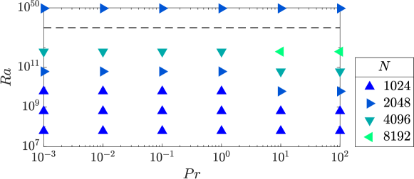
Figure 1: Parameter values simulated in the $(\mathit{Ra},\mathit{Pr})$-plane with the resolution, $N$, used at each instant colour-coded in the legend. The black dashed line separates runs with normal viscosity (below line) from those with hyperviscosity (above line).

2.2 Global and spectral quantities

Next we briefly outline the global and spectral flow properties that will be explored in our numerical simulations below. The energy spectra of the velocity field $\widehat{E}_{u}(k,t)$ and the temperature field $\widehat{E}_{\theta}(k,t)$, referred to as the kinetic energy and potential energy spectra, are defined as

$$\widehat{E}_{u}(k,t) =\frac{1}{2}\sum_{k\leq|{\bf k}|<k+\Delta k}k^{2}\left|\widehat{\psi}_{\bf k}(t)\right|^{2},$$ (6a)

$$\widehat{E}_{\theta}(k,t) =\frac{1}{2}\sum_{k\leq|{\bf k}|<k+\Delta k}\left|\widehat{\theta}_{\bf k}(t)\right|^{2},$$ (6b)

where the sum is performed over the Fourier modes with wavenumber amplitude $k=|{\bf k}|=\sqrt{k_{x}^{2}+k_{y}^{2}}$ in a shell of width $\Delta k=2\pi/L$. Using the Fourier transform, one can derive the evolution equations of kinetic and potential energy spectra from Eqs. (1), namely

$$\partial_{t}\widehat{E}_{u}(k,t) =-\partial_{k}\Pi_{u}(k,t)-D_{\nu}(k,t)-D_{\mu}(k,t)+\alpha gF_{B}(k,t),$$ (7a)

$$\partial_{t}\widehat{E}_{\theta}(k,t) =-\partial_{k}\Pi_{\theta}(k,t)-D_{\kappa}(k,t)+\frac{\Delta T}{L}F_{B}(k,t).$$ (7b)

The energy flux $\Pi$ is a measure of the nonlinear cascades in turbulence (Alexakis & Biferale, 2018). The energy flux for a circle of radius $k$ in the 2D wavenumber space is the total energy transferred from the modes within the circle to the modes outside the circle. Consequently, we define the flux of kinetic energy $\Pi_{u}(k,t)$ and potential energy $\Pi_{\theta}(k,t)$ as

$$\Pi_{u}(k,t) =\sum_{k^{\prime}\leq k}T_{u}(k^{\prime},t),$$ (8a)

$$\Pi_{\theta}(k,t) =\sum_{k^{\prime}\leq k}T_{\theta}(k^{\prime},t),$$ (8b)

where $T_{u}(k,t)$ and $T_{\theta}(k,t)$ are the non-linear kinetic and potential energy transfer across $k$:

$$T_{u}(k,t) =-\sum_{k\leq|{\bf k}|<k+\Delta k}\widehat{\psi}^{*}_{\bf k}(t)\widehat{\{\psi,\nabla^{2}\psi\}}_{\bf k}(t),$$ (9a)

$$T_{\theta}(k,t) =\sum_{k\leq|{\bf k}|<k+\Delta k}\widehat{\theta}^{*}_{\bf k}(t)\widehat{\{\psi,\theta\}}_{\bf k}(t).$$ (9b)

The notation $\widehat{\{.\}}_{\bf k}$ represents the Fourier mode of the Poisson bracket expanded using Eq. (5), and the asterisk denotes complex conjugation.

The spectra of the small-scale viscous dissipation $D_{\nu}(k,t)$, the large-scale friction $D_{\mu}(k,t)$ and the thermal dissipation $D_{\kappa}(k,t)$ are defined as

$$D_{\nu}(k,t) =2\nu k^{2n}\widehat{E}_{u}(k,t),$$ (10a)

$$D_{\mu}(k,t) =2\mu k^{-2}\widehat{E}_{u}(k,t),$$ (10b)

$$D_{\kappa}(k,t) =2\kappa k^{2n}\widehat{E}_{\theta}(k,t),$$ (10c)

and the buoyancy term $F_{B}$ is given by

$$F_{B}(k,t) =\sum_{k\leq|{\bf k}|<k+\Delta k}ik_{x}\widehat{\psi^{*}}_{\bf k}(t)\widehat{\theta}_{\bf k}(t).$$ (11)

The Nusselt number is a dimensionless measure of the averaged vertical heat flux, defined mathematically by

$$\mathit{Nu}=1+\frac{\langle{\partial_{x}\psi\,\theta}\rangle}{\kappa\Delta T/L^{2n-1}}.$$ (12)

Using the above definition, one can derive the following exact relations for the kinetic and potential energy balances in the statistically stationary regime, as in Shraiman & Siggia (1990):

$$\epsilon_{u} =\epsilon_{\nu}+\epsilon_{\mu}=\frac{\nu^{3}}{L^{6n-2}}(\mathit{Nu}-1)\frac{\mathit{Ra}}{\mathit{Pr}^{2}}$$ (13a)

$$\epsilon_{\theta} =\epsilon_{\kappa}=\frac{\kappa\Delta T^{2}}{L^{2n}}(\mathit{Nu}-1)$$ (13b)

where $\epsilon_{u}=\alpha g\langle{\psi\,\partial_{x}\theta}\rangle$ is the injection rate of kinetic energy due to buoyancy, $\epsilon_{\nu}=\nu{\langle\psi\nabla^{2(n+1)}\psi\rangle}$ is the viscous dissipation rate, $\epsilon_{\mu}=\mu{\langle\psi^{2}\rangle}$ is the large scale dissipation rate, $\epsilon_{\theta}=\frac{\Delta T}{L}\langle{\partial_{x}\psi\,\theta}\rangle$ is the injection rate of potential energy due to buoyancy and $\epsilon_{\kappa}=\kappa{\langle\theta\nabla^{2n}\theta\rangle}$ is the thermal dissipation rate.

2.3 Elevator modes

Upon linearising (1) about the conductive state ($\psi=\theta=0$), we find that infinitesimal solutions with $\psi(\mathbf{x},t)=e^{i\mathbf{k}\cdot\mathbf{x}+\sigma t}$ are possible provided the normalised linear growth rate $\sigma$ satisfies the relation

$$\left(\sigma+k^{2n}\right)\left(\sigma+\mathit{Pr}k^{2n}+\frac{\mathit{Rh}\sqrt{\mathit{Ra}\mathit{Pr}}}{k^{2}}\right)=\frac{\mathit{Ra}\mathit{Pr}(2\pi k_{x})^{2}}{k^{2}},$$ (14)

which has two real roots for $\sigma$. From these two roots, one is positive if and only if

$$\mathit{Rh}\sqrt{\frac{\mathit{Ra}}{\mathit{Pr}}}<\frac{\mathit{Ra}(2\pi k_{x})^{2}}{k^{2n}}-k^{2n+2}.$$ (15)

One can show that $\sigma$ is a monotonic decreasing function of $k_{y}$, so the most dangerous modes are independent of $y$, with

$$\psi(\mathbf{x},t)=e^{ik_{x}x+\sigma t},\qquad k_{x}\in\mathbb{Z}_{>0}.$$ (16)

Indeed, such a unidirectional mode satisfies the nonlinear governing equations (1) exactly (because the nonlinear Poisson bracket terms are identically zero).

Although the maximum growth rate does not necessarily occur at the minimum wavenumber $k_{x}=1$, it is straightforward to show that (15) is satisfied for some $(k_{x},k_{y})$ if and only if it is satisfied at $(k_{x},k_{y})=(1,0)$. In other words, exact solutions of the problem (1) that grow exponentially without bound exist whenever

$$\mathit{Rh}\sqrt{\frac{\mathit{Ra}}{\mathit{Pr}}}<\frac{\mathit{Ra}}{(2\pi)^{2(n-1)}}-(2\pi)^{2n+2}.$$ (17)

3 Results

3.1 Zero and infinite Prandtl number

Before considering the $\mathit{Pr}\to\infty$ limit, to simplify the analysis let’s write the non-dimensional form of Eqs. (1) in accordance with Eqs. (4), which yield

$$\partial_{t}\nabla^{2}\psi+\{\psi,\nabla^{2}\psi\} =\mathit{Ra}\mathit{Pr}\partial_{x}\theta+\mathit{Pr}(-1)^{n+1}\nabla^{2(n+1)}\psi+\mathit{Rh}\sqrt{\frac{\mathit{Ra}}{\mathit{Pr}}}\,\psi,$$ (18a)

$$\partial_{t}\theta+\{\psi,\theta\} =\partial_{x}\psi+(-1)^{n+1}\nabla^{2n}\theta.$$ (18b)

As we take $\mathit{Pr}$ to infinity, we ensure that $\mathit{Rh}\sqrt{\mathit{Ra}/\mathit{Pr}}$ is finite to maintain the effects of the large-scale dissipation. The system (18) thus reduces to

$$\mathit{Ra}\partial_{x}\theta =\left[(-1)^{n}\nabla^{2(n+1)}-\mathit{Rh}\sqrt{\frac{\mathit{Ra}}{\mathit{Pr}}}\right]\psi,$$ (19a)

$$\partial_{t}\theta+\{\psi,\theta\} =\partial_{x}\psi+(-1)^{n+1}\nabla^{2n}\theta.$$ (19b)

In the complementary limit of zero Prandtl number, we have to rescale the variables according to

$$\{\psi,\theta,t\}\mapsto\{\mathit{Pr}\,\psi,\mathit{Pr}\,\theta,t/\mathit{Pr}\}$$ (20)

before letting $\mathit{Pr}\to 0$, which removes the time derivative and advective term from the heat transport equation (18b). As in the $\mathit{Pr}\to\infty$ case, we maintain the effects of the large-scale dissipation by ensuring that $\mathit{Rh}\sqrt{\mathit{Ra}/\mathit{Pr}}$ is finite. This process reduces the system (18) to

$$\partial_{t}\nabla^{2}\psi+\{\psi,\nabla^{2}\psi\} =\mathit{Ra}\partial_{x}\theta+(-1)^{n+1}\nabla^{2(n+1)}\psi+\mathit{Rh}\sqrt{\frac{\mathit{Ra}}{\mathit{Pr}}}\psi,$$ (21a)

$$\partial_{x}\psi =(-1)^{n}\nabla^{2n}\theta.$$ (21b)

In Figure 2 we plot time series of the kinetic energy, $E_{u}$ in both the $\mathit{Pr}\to 0$ and $\mathit{Pr}\to\infty$ limits. We use normal viscosity (i.e. $n=1$), we set $\mathit{Ra}=10^{7}$ for four different values of $\mathit{Rh}\sqrt{\mathit{Ra}/\mathit{Pr}}$, and the simulations are initialised with random initial data. The flow converges to a statistically steady state only in the case where $\mathit{Pr}\to\infty$ and $\mathit{Rh}\sqrt{\mathit{Ra}/\mathit{Pr}}=9\times 10^{6}$, a value only $10\%$ smaller than the maximum value given by (17) at which all convection is suppressed. For all other parameter values attempted, an elevator mode takes over the dynamics and the energy grows without bound.

At present, we are not able to reliably obtain turbulent saturated states in the extreme Prandtl number limits, unless the large-scale dissipation is made very strong. Instead, for the remainder of the paper we restrict our attention to finite values of Prandtl number, for which we find that $\mathit{Rh}=(2\pi)^{5/2}$ is sufficient to prevent elevator modes and allow the system to reach turbulent saturated states.

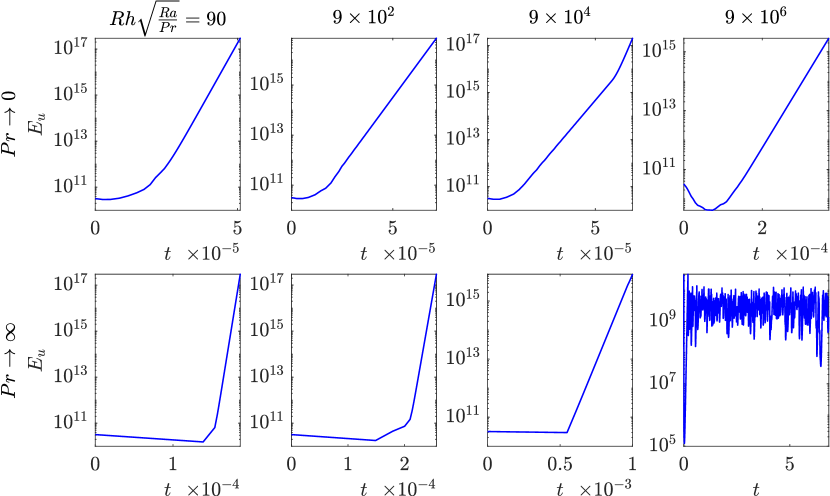
Figure 2: Time series of the kinetic energy, $E_{u}$, in the $\mathit{Pr}\to 0$ and $\mathit{Pr}\to\infty$ limits with normal viscosity ($n=1$), at $\mathit{Ra}=10^{7}$ and four different values of $\mathit{Rh}\sqrt{\mathit{Ra}/\mathit{Pr}}$. The time series are initiated with random initial conditions.

3.2 Finite Prandtl number: global variables

In Fig. 3(a)–(c) we show how the global quantities in the kinetic and potential energy balances (13) vary with $\mathit{Pr}$ keeping $\mathit{Ra}=6.2\times 10^{11}$, while in (d)–(f) we show how the same quantities vary with $\mathit{Ra}$ while keeping $\mathit{Pr}=1$. In both cases we use normal viscosity ($n=1$) and keep $\mathit{Rh}=(2\pi)^{5/2}$ constant. Firstly, Fig. 3(a) and (d) show that the kinetic and potential energies remain virtually constant while $\mathit{Pr}$ and $\mathit{Ra}$ vary by at least four orders of magnitude. Secondly, Fig. 3(b) and (e) show that $\epsilon_{u}\approx\epsilon_{\mu}$, which indicates that the majority of the kinetic energy, injected by buoyancy in the flow, is dissipated at large scales. This effect is caused by the inverse cascade of kinetic energy, which will be investigated in more detail in Sec. 3.3. Note that $\epsilon_{u}$ and $\epsilon_{\mu}$ are almost independent of both $\mathit{Pr}$ and $\mathit{Ra}$, while the viscous dissipation scales like

$$\epsilon_{\nu}\propto\mathit{Pr}^{1/2}\mathit{Ra}^{-1/4}.$$ (22)

Finally, in Fig. 3(c) and (f), we see that $\epsilon_{\theta}=\epsilon_{\kappa}$, as required by the potential energy balance (13b), and both quantities, are also virtually independent of both $\mathit{Pr}$ and $\mathit{Ra}$.

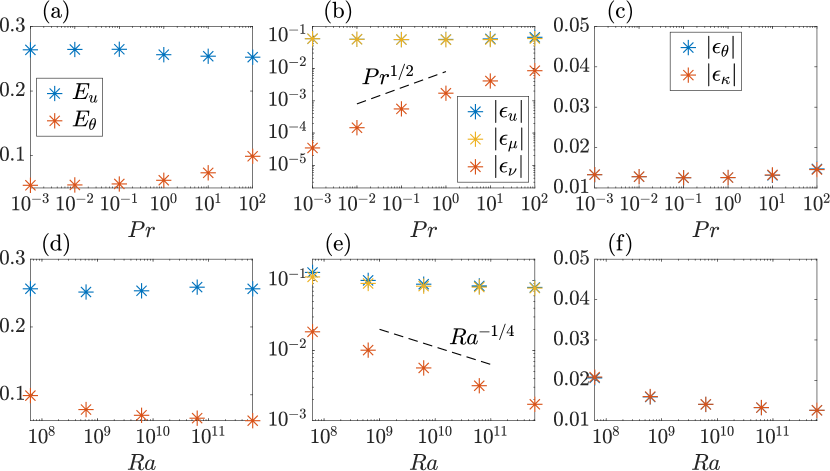
Figure 3: Spatiotemporal averages of the kinetic and potential energies and the terms in the kinetic and potential energy balances (13) as functions of $\mathit{Pr}$ with $\mathit{Ra}=6.2\times 10^{11}$ fixed (a–c) and as functions of $\mathit{Ra}$ with $\mathit{Pr}=1$ fixed (d–f). We use normal viscosity ($n=1$) and keep $\mathit{Rh}=(2\pi)^{5/2}$ fixed in all plots.

To explain the scaling of the viscous dissipation rate (22), we now look at how the enstrophy $\langle{\omega^{2}}\rangle$ varies with the Prandtl and Rayleigh numbers, where $\omega=\nabla^{2}\psi$ is the vorticity of the flow. In Fig. 4(a) we plot enstrophy as a function of $\mathit{Pr}$ with $\mathit{Ra}=6.2\times 10^{11}$ fixed, and in Fig. 4(b) as a function of $\mathit{Ra}$ with $\mathit{Pr}=1$ fixed. We keep $\mathit{Rh}=(2\pi)^{5/2}$ fixed throughout. From Fig. 4(a) we observe that enstrophy can be considered approximately independent of $\mathit{Pr}$, because it varies by less than a factor of two over the five decades of Prandtl numbers considered, while Fig. 4(b) demonstrates that enstrophy scales like $\mathit{Ra}^{1/4}$, i.e.,

$$\langle{\omega^{2}}\rangle\propto\mathit{Pr}^{0}\mathit{Ra}^{1/4}.$$ (23)

With normal viscosity, by definition we have $\epsilon_{\nu}=\nu\langle{\psi\nabla^{4}\psi}\rangle=\nu\langle{\omega^{2}}\rangle$ and, writing $\nu\propto(\mathit{Pr}/\mathit{Ra})^{1/2}$, we thus obtain the scaling of Eq. (22) that is observed in Fig. 3.

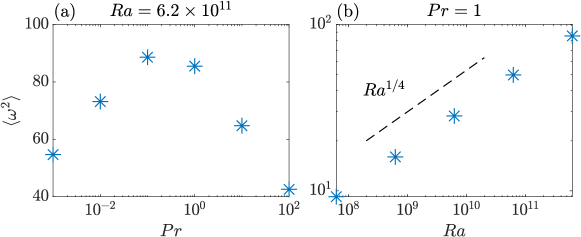
Figure 4: Enstrophy $\langle{\omega^{2}}\rangle$ as a function of $\mathit{Pr}$ with $\mathit{Ra}=6.2\times 10^{11}$ fixed (a), and as a function of $\mathit{Ra}$ with $\mathit{Pr}=1$ fixed (b). We keep $n=1$ (normal viscosity) and $\mathit{Rh}=(2\pi)^{5/2}$ fixed in all plots.

According to Fig. 3, the normalised energy injection rates $\epsilon_{u}$ and $\epsilon_{\theta}$ are both approximately constant in the range of $\mathit{Pr}$ and $\mathit{Ra}$ we considered. With $\mathit{Ra}\mathit{Pr}\gg 1$ and $n=1$, the net energy balances (13) thus produce the Nusselt number scaling

$$\mathit{Nu}\propto\mathit{Pr}^{1/2}\mathit{Ra}^{1/2}.$$ (24)

This relation is in agreement with the ultimate scaling. In Fig. 5, we plot the Nusselt number compensated by the classical scaling, $\mathit{Nu}\propto\mathit{Pr}^{0}\mathit{Ra}^{1/3}$, and by the ultimate scaling, $\mathit{Nu}\propto\mathit{Pr}^{1/2}\mathit{Ra}^{1/2}$. The ultimate scaling provides a much more convincing collapse of the data, with the fit becoming increasingly accurate as $\mathit{Ra}$ increases.

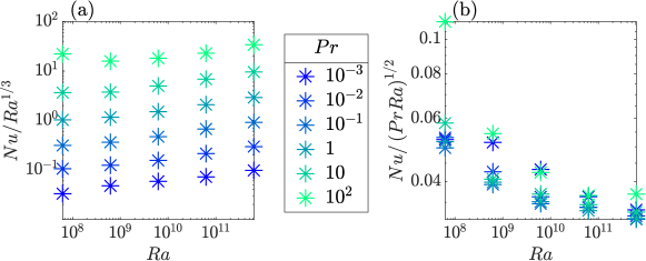
Figure 5: The Nusselt number compensated with the ‘classical’ and the ‘ultimate’ scaling in (a) and (b), respectively. The Prandtl numbers are colour-coded in the legend.

Indeed, the ultimate scaling in terms of Rayleigh number dependence was expected to be exhibited by our simulations as we have effectively removed the boundary layers by applying periodic boundary conditions on the computational domain (Lohse & Toschi, 2003; Calzavarini et al., 2005; Schmidt et al., 2012). In addition, we demonstrate that the Prandtl number dependence follows the ultimate scaling, too.

3.3 Finite Prandtl number: spectra

In this section, we examine the time-averaged kinetic and potential energy spectra and spectral fluxes. To eliminate finite Rayleigh number effects and to have large enough scale separation, we focus on the hyperviscous simulations (i.e., $n=4$ in Eqs. (1)) at $\mathit{Ra}=9.4\times 10^{49}$ and $\mathit{Rh}=(2\pi)^{5/2}$. Results with normal viscosity (i.e. $n=1$ in Eqs. (1)) at $\mathit{Ra}=6.2\times 10^{11}$ are also presented for comparison. According to the Bolgiano–Obukhov (BO) scaling (Bolgiano Jr., 1959; Obukhov, 1959), the ratio of the kinetic to the potential energy spectra scales as $\widehat{E}_{u}(k)/\widehat{E}_{\theta}(k)\propto k^{-4/5}$, since $\widehat{E}_{u}\propto k^{-11/5}$ and $\widehat{E}_{\theta}\propto k^{-7/5}$. In Fig. 6 we plot $\widehat{E}_{u}(k)/\widehat{E}_{\theta}(k)$ compensated by $k^{4/5}$ for the hyperviscous simulations and, in the inset, for the runs with normal viscosity. Instead of finding a wavenumber range where this scaling is valid, we observe a $k^{-0.3}$ power-law in the inertial range for all Prandtl numbers considered, leading us to the conclusion that BO scaling is not followed in our simulations. For the normal viscosity simulations we find the $k^{-0.3}$ power-law again to be followed, but within a narrower wavenumber range (see inset of Fig. 6). Fig. 6 also shows that, for $\mathit{Pr}\ll 1$, the kinetic energy is much larger than the potential energy at large wavenumbers. This is expected as the small scales are dominated by thermal diffusivity when $\mathit{Pr}\ll 1$ and so the potential energy is dissipated much more effectively than the kinetic energy. The opposite is true for $\mathit{Pr}\gg 1$.

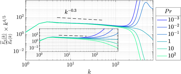
Figure 6: The ratio of the kinetic energy to the potential energy spectra $\widehat{E}_{u}(k)/\widehat{E}_{\theta}(k)$ compensated by $k^{4/5}$ for the hyperviscous simulations with $\mathit{Ra}=9.4\times 10^{49}$, $\mathit{Rh}=(2\pi)^{5/2}$ and different Prandtl numbers as colour-coded in the legend. The inset shows the same ratio but for runs with normal viscosity at $\mathit{Ra}=6.2\times 10^{11}$.

In Fig. 7(a) and (b), we plot the kinetic and potential energy spectra multiplied by powers of $k$ chosen to best compensate for the power-laws exhibited by the spectra. The hyperviscous runs are shown in the main plots, and normal viscosity runs in the insets. The observed behaviour, with $\hat{E}_{u}(k)\propto k^{-2.3}$ and $\hat{E}_{\theta}(k)\propto k^{-1.2}$, is close to, but not fully consistent with, BO phenomenology, according to which the exponents should be $-11/5=-2.2$ and $-7/5=-1.4$, respectively. Moreover, the spectra we observe are in contrast to 3D RBC with periodic boundary conditions, where the kinetic and potential energy exhibit $k^{-5/3}$ spectra (Borue & Orszag, 1997), similar to those observed in passive scalar turbulence (Warhaft, 2000).

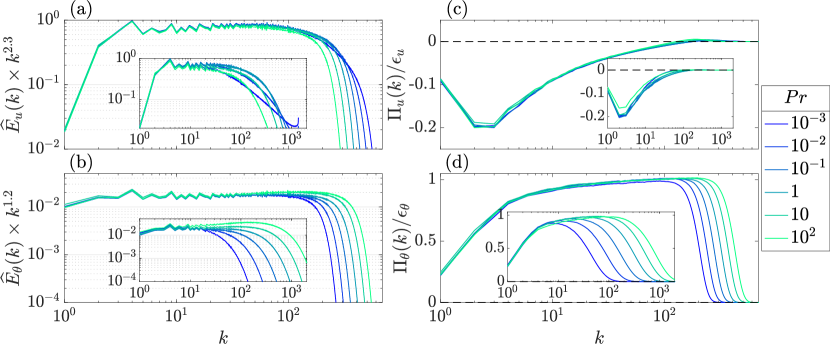
Figure 7: The time averaged energy spectra compensated by best fit power laws (a,b), and spectral fluxes normalised by the time-averaged dissipation rates (c,d) for the runs with hyperviscosity at $\mathit{Ra}=9.4\times 10^{49}$, $\mathit{Rh}=(2\pi)^{5/2}$ and different Prandtl numbers as colour-coded in the legend. The insets shows the same quantities but for runs with normal viscosity at $\mathit{Ra}=6.2\times 10^{11}$.

To understand the turbulent cascades, in Fig. 7(c) and (d), we plot the associated kinetic and potential energy fluxes normalised by the time-averaged injection rates of energy due to buoyancy. The positive potential energy flux suggests a strong direct cascade, while there is a weak inverse cascade of kinetic energy, which is typical for 2D turbulence (Alexakis & Biferale, 2018). For $\mathit{Pr}=1$ these types of cascades are in agreement with Xie & Huang (2022). The negative kinetic energy flux peaks at low wavenumbers, while the potential energy flux peaks at high wavenumbers. The inverse cascade of kinetic energy is not affected by the Prandtl number; however, the direct cascade of potential energy moves to higher wavenumbers along with the peak of $\Pi_{\theta}(k)$ as $\mathit{Pr}$ increases. We emphasise the wavenumber dependence of kinetic and potential energy fluxes, with $\partial_{k}\Pi_{u}(k)>0$ and $\partial_{k}\Pi_{\theta}(k)>0$ in the inertial range of wavenumbers for all of the Prandtl numbers considered.

In Fig. 8, we present the time-averaged spectra of the magnitudes of the terms in the kinetic and potential energy balances (7) for runs with hyperviscosity and three different values of $\mathit{Pr}\in\left\{10^{-2},1,10^{2}\right\}$. The corresponding plots with normal viscosity and $\mathit{Ra}=6.2\times 10^{11}$ are shown in Fig. 9. In both figures, the red dots indicate where the inertial flux terms $\partial_{k}\Pi_{u}$ and $\partial_{k}\Pi_{\theta}$ become negative. In the kinetic energy balance, we identify three distinct wavenumber ranges, labeled I to III in the plots. In region I, the kinetic energy injected by buoyancy is dissipated by the large-scale friction. In region II, the inertial term balances buoyancy, which is positive for all wavenumbers in this region, i.e.

$$\partial_{k}\Pi_{u}(k)\approx\alpha gF_{B}(k)>0.$$ (25)

This relation shows how the kinetic energy injected by buoyancy is cascaded to larger scales in the inertial range of wavenumbers and explains the $k$ dependence of the kinetic energy flux we see in Fig. 7(c). Note that region II is largest for small Prandtl numbers, especially in the runs with normal viscosity, as evident from the results presented in Fig. 9(a)–(c). In region III, the balances between terms depend on the Prandtl number. For $\mathit{Pr}=10^{-2}$ buoyancy decays rapidly and so small-scale viscous dissipation is balanced by the inertial term, which is negative in this range of wavenumbers. As $\mathit{Pr}$ increases, buoyancy becomes more significant in the balance of region III between the small-scale viscous dissipation and the inertial term. For $\mathit{Pr}\gtrsim 10^{2}$, small-scale viscous dissipation seems to be balanced by buoyancy rather than by the inertial term. This effect is shown more clearly in the runs with normal viscosity shown in Fig. 9(c), where the small-scale dissipation range is much larger.

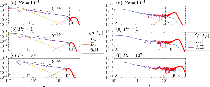
Figure 8: Time-averaged spectra of the terms in the kinetic energy balance (7a) (a)–(c); and the potential energy balance (7b) (d)–(f) for the runs with hyperviscosity, $\mathit{Ra}=9.4\times 10^{49}$, $\mathit{Rh}=(2\pi)^{5/2}$, and $\mathit{Pr}=10^{-2}$ (a), (d), $\mathit{Pr}=1$ (b), (e), and $\mathit{Pr}=10^{2}$ (c), (f). The terms displayed in the legends are defined in (8), (10) and (11). In (a)–(c) and (d)–(f), we observe three and two distinct dominant balances, respectively, annotated I–III and A–B. The red dots indicate where the inertial terms become negative.

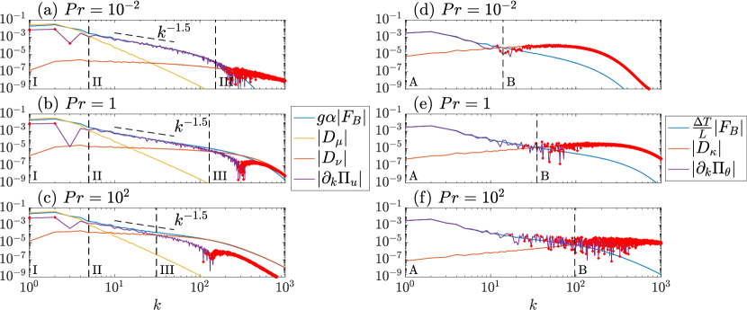
Figure 9: Time-averaged spectra of the terms in the kinetic energy balance (7a) (a)–(c); and the potential energy balance (7b) (d)–(f) for the runs with normal viscosity, $\mathit{Ra}=6.2\times 10^{11}$, $\mathit{Rh}=(2\pi)^{5/2}$, and $\mathit{Pr}=10^{-2}$ (a), (d), $\mathit{Pr}=1$ (b), (e), and $\mathit{Pr}=10^{2}$ (c), (f). The terms displayed in the legend are defined in (8), (10) and (11). In (a)–(c) and (d)–(f), we observe three and two distinct dominant balances, respectively, annotated I–III and A–B. The red dots indicate where the inertial terms become negative.

In the potential energy balance, we identify two distinct wavenumber ranges, labeled A and B in the plots (see (d)–(f) in Plots. 8 and 9). In these plots we observe the inertial term to be balanced by buoyancy in region A and by small- scale thermal dissipation in region B. In other words, the potential energy injected by buoyancy in region A is cascaded to larger wavenumbers, where it is dissipated by thermal diffusivity.

We recall that the red dots in Plots. 8 and 9 show where the inertial terms of the kinetic and potential energy become negative. This sign change occurs primarily in region III for $\partial_{k}\Pi_{u}(k)$ and region B for $\partial_{k}\Pi_{\theta}(k)$, the latter corresponding to the large negative gradient of $\Pi_{\theta}(k)$ observed in Fig. 7 at large wavenumbers. Near the boundary between regions A and B in Plots. 8 and 9(d)–(f), we observe that $\partial_{k}\Pi_{\theta}(k)$ exhibits fluctuations between positive and negative values over these wavenumbers. However, for the majority of the wavenumbers in region A we find that

$$\partial_{k}\Pi_{\theta}(k)\approx\frac{\Delta T}{L}F_{B}(k)>0.$$ (26)

This relation explains the $k$ dependence of the potential energy flux we observe in Fig. 7(d) and demonstrates that the BO phenomenology, which assumes that the potential energy flux is constant in the inertial range of wavenumbers, does not hold for any of the Prandtl numbers we studied. Note that in the wavenumber range where region II and A overlap, we have $\partial_{k}\Pi_{u}(k)/\alpha g\approx L\partial_{k}\Pi_{\theta}(k)/\Delta T\approx F_{B}(k)$, such that $\Pi_{u}(k)-\frac{\alpha gL}{\Delta T}\Pi_{\theta}(k)$ is approximately constant for all Prandtl numbers considered. This is the inertial range of scales, where the viscous, diffusive and friction effects can be neglected and so the energy flux is constant. This is expected for the quantity $E_{u}-\frac{agL}{\Delta T}E_{\theta}$, which is constant in the limit of $\nu\to 0$, $\kappa\to 0$, and $\mu\to 0$.

4 Conclusions

In this paper we study the effects of varying the Prandtl and Rayleigh numbers on the dynamics of two-dimensional Rayleigh-Bénard convection without boundaries, i.e., with periodic boundary conditions. First, we focus on the limits of $\mathit{Pr}\to 0$ and $\mathit{Pr}\to\infty$. Our findings indicate that, unless large-scale dissipation is made so strong as to almost suppress convection completely, large-scale elevator modes dominate the dynamics. Such elevator modes have long been known (Baines & Gill, 1969). In all parameter values simulated, the inequality (17) is violated, implying that the system admits exact single-mode solutions that grow exponentially without bound. Instead, we turn to finite Prandtl numbers, where we find that non-linear interactions between modes continue to allow the system to find a turbulent stationary state. In general, whether or not the solution blows up must depend on the initial conditions, in a way that is not currently understood.

Examining the Prandtl and Rayleigh number dependence of the terms in the kinetic and potential energy balances, we find that the enstrophy scales as $\langle{\omega^{2}}\rangle\propto\mathit{Pr}^{0}\mathit{Ra}^{1/4}$ and hence the small-scale viscous dissipation scales as $\epsilon_{\nu}=\nu\langle{\omega^{2}}\rangle\propto\mathit{Pr}^{1/2}\mathit{Ra}^{-1/4}$. On the other hand, we observe that the injection rate of kinetic energy $\epsilon_{u}$ due to buoyancy is effectively independent of both the Prandtl and the Rayleigh number. Using this observation, we find that $\mathit{Nu}\propto\mathit{Pr}^{1/2}\mathit{Ra}^{1/2}$, which agrees with the so-called ultimate scaling.

Looking at the kinetic and potential energy spectral fluxes, we find an inverse cascade of kinetic energy and a direct cascade of potential energy in contrast to 3D RBC (Verma, 2018), where both kinetic and potential energies cascade toward small scales. The inverse cascade is independent of the Prandtl number, while the peak of the potential energy flux moves to higher wavenumbers as $\mathit{Pr}$ increases. The kinetic and potential energy fluxes, $\Pi_{u}(k)$ and $\Pi_{\theta}(k)$, are not constant in the inertial range because both are balanced by the buoyancy term $F_{B}(k)$, which is predominantly positive in this range of wavenumbers. These two balances imply a positive slope in $k$ for the fluxes. Although we observe no range of wavenumbers where either $\Pi_{u}(k)$ or $\Pi_{\theta}(k)$ is constant, we find that they are connected by the relation $\Pi_{u}(k)-\frac{\alpha gL}{\Delta T}\Pi_{\theta}(k)\approx\text{constant}$ in the overlap between regions II and A shown in Plots. 8 and 9.

The kinetic energy spectra scale as $\widehat{E}_{u}(k)\propto k^{-2.3}$, which is close to $k^{-11/5}$ behaviour of the BO phenomenology. However, the potential energy spectra scale as $\widehat{E}_{\theta}(k)\propto k^{-1.2}$, which deviates significantly from the $k^{-7/5}$ scaling predicted by the BO arguments. The deviation from the BO phenomenology is clearer when we test the scaling $\widehat{E}_{u}(k)/\widehat{E}_{\theta}(k)k^{4/5}\approx\text{constant}$, which is clearly not followed by our spectra which follow $\widehat{E}_{u}(k)/\widehat{E}_{\theta}(k)k^{4/5}\propto k^{-0.3}$. For the hyperviscous simulations, the observed power-laws in the inertial range of the kinetic and potential energy spectra do not show any dependence on the Prandtl number. The only dependence we observe is at the dissipative range of wavenumbers, where the viscosity and the thermal diffusivity dominate the dynamics. In the spectra from the normal viscosity simulations, the effects of the Prandtl number are more significant due to the comparatively low scale separation. Hence, the inertial range over which a power-law behaviour can be observed is truncated.

This study clearly demonstrates the necessity for large scale separation to be able to make clearer conclusions on the spectral dynamics and the power-law exponents of two-dimensional Rayleigh-Bénard convection. This requirement makes similar studies in three dimensions more challenging. The development of a phenomenology where buoyancy acts as a broadband spectral forcing is required to interpret the current observations. Numerical simulations at Prandtl and Rayleigh numbers outside the ranges we investigated, i.e., $\mathit{Pr}<10^{-3}$, $\mathit{Pr}>10^{2}$ and $\mathit{Ra}>10^{12}$, are challenging but would be of great interest to see if they agree with the hyperviscous simulations we have performed and to provide a more complete picture of the asymptotic regime of buoyancy driven turbulent convection.

References

- Alexakis & Biferale (2018) Alexakis, A. & Biferale, L. 2018 Cascades and transitions in turbulent flows. Physics Reports 767-769, 1–101, cascades and transitions in turbulent flows.
- Baines & Gill (1969) Baines, PG & Gill, AE 1969 On thermohaline convection with linear gradients. Journal of Fluid Mechanics 37 (2), 289–306.
- Barral & Dubrulle (2023) Barral, Amaury & Dubrulle, Berengere 2023 Asymptotic ultimate regime of homogeneous rayleigh–bénard convection on logarithmic lattices. Journal of Fluid Mechanics 962, A2.
- Batchelor & Nitsche (1991) Batchelor, GK & Nitsche, JM 1991 Instability of stationary unbounded stratified fluid. Journal of fluid mechanics 227, 357–391.
- Bénard (1900) Bénard, H 1900 Etude expérimentale du mouvement des liquides propageant de la chaleur par convection. Régime permanent: tourbillons cellulaires. C. r. hebd. séances Acad. sci. Paris 130, 1004–1007.
- Bénard (1927) Bénard, H 1927 Sur les tourbillons cellulaires et la théorie de Rayleigh. C. r. hebd. séances Acad. sci. Paris 185, 1109–1111.
- Biskamp et al. (2001) Biskamp, D., Hallatschek, K. & Schwarz, E. 2001 Scaling laws in two-dimensional turbulent convection. Phys. Rev. E 63, 045302.
- Biskamp & Schwarz (1997) Biskamp, D. & Schwarz, E. 1997 Scaling properties of turbulent convection in two-dimensional periodic systems. Europhysics Letters 40 (6), 637.
- Boffetta & Ecke (2012) Boffetta, Guido & Ecke, Robert E 2012 Two-dimensional turbulence. Annual review of fluid mechanics 44, 427–451.
- Bolgiano Jr. (1959) Bolgiano Jr., R. 1959 Turbulent spectra in a stably stratified atmosphere. Journal of Geophysical Research (1896-1977) 64 (12), 2226–2229.
- Borue & Orszag (1997) Borue, Vadim & Orszag, Steven A 1997 Turbulent convection driven by a constant temperature gradient. Journal of Scientific computing 12, 305–351.
- Boussinesq (1903) Boussinesq, Joseph 1903 Théorie analytique de la chaleur mise en harmonic avec la thermodynamique et avec la théorie mécanique de la lumière, , vol. II. Gauthier-Villars.
- Calzavarini et al. (2006) Calzavarini, E., Doering, C. R., Gibbon, J. D., Lohse, D., Tanabe, A. & Toschi, F. 2006 Exponentially growing solutions in homogeneous rayleigh-bénard convection. Phys. Rev. E 73, 035301.
- Calzavarini et al. (2005) Calzavarini, Enrico, Lohse, Detlef, Toschi, Federico & Tripiccione, Raffaele 2005 Rayleigh and prandtl number scaling in the bulk of rayleigh–bénard turbulence. Physics of fluids 17 (5), 055107.
- Calzavarini et al. (2002) Calzavarini, Enrico, Toschi, Federico & Tripiccione, Raffaele 2002 Evidences of bolgiano-obhukhov scaling in three-dimensional rayleigh-benard convection. Physical review. E, Statistical, nonlinear, and soft matter physics 66, 016304.
- Celani et al. (2002) Celani, Antonio, Matsumoto, Takeshi, Mazzino, Andrea & Vergassola, Massimo 2002 Scaling and universality in turbulent convection. Phys. Rev. Lett. 88, 054503.
- Celani et al. (2001) Celani, A, Mazzino, A & Vergassola, M 2001 Thermal plume turbulence. Physics of fluids 13 (7), 2133–2135.
- Chavanne et al. (2001) Chavanne, X., Chillà, F., Chabaud, B., Castaing, B. & Hébral, B. 2001 Turbulent rayleigh–bénard convection in gaseous and liquid he. Physics of Fluids 13 (5), 1300–1320.
- Chertkov et al. (2007) Chertkov, M., Connaughton, C., Kolokolov, I. & Lebedev, V. 2007 Dynamics of energy condensation in two-dimensional turbulence. Phys. Rev. Lett. 99, 084501.
- Doering (2019) Doering, Charles R 2019 Thermal forcing and ‘classical’and ‘ultimate’regimes of rayleigh–bénard convection. Journal of Fluid Mechanics 868, 1–4.
- Doering et al. (2019) Doering, C. R., Toppaladoddi, S. & Wettlaufer, J. S. 2019 Absence of evidence for the ultimate regime in two-dimensional rayleigh-bénard convection. Phys. Rev. Lett. 123, 259401.
- Gómez et al. (2005) Gómez, D. O., Mininni, P. D. & Dmitruk, P. 2005 Parallel simulations in turbulent MHD. Physica Scripta T116, 123–127.
- He et al. (2021) He, Jian-Chao, Fang, Ming-Wei, Gao, Zhen-Yuan, Huang, Shi-Di & Bao, Yun 2021 Effects of prandtl number in two-dimensional turbulent convection. Chinese Physics B 30 (9), 094701.
- He et al. (2012) He, Xiaozhou, Funfschilling, Denis, Nobach, Holger, Bodenschatz, Eberhard & Ahlers, Guenter 2012 Transition to the ultimate state of turbulent rayleigh-bénard convection. Phys. Rev. Lett. 108 (2).
- Kaczorowski & Xia (2013) Kaczorowski, Matthias & Xia, Ke-Qing 2013 Turbulent flow in the bulk of rayleigh–bénard convection: small-scale properties in a cubic cell. Journal of Fluid Mechanics 722, 596–617.
- Kolmogorov (1941) Kolmogorov, Andrey 1941 The local structure of turbulence in incompressible viscous fluid for very large reynolds’ numbers. Comptes Rendus (Doklady) de l’Académie des Sciences de l’URSS, Nouvelle Série 30.
- Kraichnan (1962) Kraichnan, Robert H. 1962 Turbulent thermal convection at arbitrary prandtl number. Physics of Fluids 5 (11), 1374.
- Kunnen & Clercx (2014) Kunnen, RPJ & Clercx, HJH 2014 Probing the energy cascade of convective turbulence. Physical Review E 90 (6), 063018.
- Lepot et al. (2018) Lepot, Simon, Aumaître, Sébastien & Gallet, Basile 2018 Radiative heating achieves the ultimate regime of thermal convection. Proceedings of the National Academy of Sciences 115 (36), 8937–8941.
- Liu & Zikanov (2015) Liu, Li & Zikanov, Oleg 2015 Elevator mode convection in flows with strong magnetic fields. Physics of Fluids 27 (4).
- Lohse & Toschi (2003) Lohse, Detlef & Toschi, Federico 2003 Ultimate state of thermal convection. Phys. Rev. Lett. 90, 034502.
- Lohse & Xia (2010) Lohse, Detlef & Xia, Ke-Qing 2010 Small-scale properties of turbulent rayleigh-bénard convection. Annual Review of Fluid Mechanics 42 (1), 335–364.
- Malkus (1954) Malkus, Willem VR 1954 The heat transport and spectrum of thermal turbulence. Proceedings of the Royal Society of London. Series A. Mathematical and Physical Sciences 225 (1161), 196–212.
- Mazzino (2017) Mazzino, Andrea 2017 Two-dimensional turbulent convection. Physics of Fluids 29 (11), 111102.
- Mishra & Verma (2010) Mishra, Pankaj Kumar & Verma, Mahendra K. 2010 Energy spectra and fluxes for rayleigh-bénard convection. Phys. Rev. E 81, 056316.
- Ng et al. (2018) Ng, Chong Shen, Ooi, Andrew, Lohse, Detlef & Chung, Daniel 2018 Bulk scaling in wall-bounded and homogeneous vertical natural convection. Journal of fluid mechanics 841, 825–850.
- Niemela et al. (2000) Niemela, J. J., Skrbek, L., Sreenivasan, K. R. & Donnelly, R. J. 2000 Turbulent convection at very high rayleigh numbers. Nature 404 (6780), 837–840.
- Niemela & Sreenivasan (2003) Niemela, J. J. & Sreenivasan, K. R. 2003 Confined turbulent convection. Journal of Fluid Mechanics 481, 355–384.
- Oberbeck (1879) Oberbeck, Anton 1879 Über die Wärmeleitung der Flüssigkeiten bei Berücksichtigung der Strömungen infolge von Temperaturdifferenzen. Ann. Phys. Chem. 243 (6), 271–292.
- Obukhov (1959) Obukhov, A. M. 1959 On influence of buoyancy forces on the structure of temperature field in a turbulent flow. Dokl. Akad. Nauk. SSR 125, 1246–48.
- Orszag & Gottlieb (1977) Orszag, S. A. & Gottlieb, D. 1977 Numerical analysis of spectral methods: theory and application. SIAM.
- Rayleigh (1916) Rayleigh, Lord 1916 On convection currents in a horizontal layer of fluid, when the higher temperature is on the under side. Phil. Mag. S. 32 (192), 529–546.
- Schmidt et al. (2012) Schmidt, Laura E, Calzavarini, Enrico, Lohse, Detlef, Toschi, Federico & Verzicco, Roberto 2012 Axially homogeneous rayleigh–bénard convection in a cylindrical cell. Journal of fluid mechanics 691, 52–68.
- Shraiman & Siggia (1990) Shraiman, Boris I & Siggia, Eric D 1990 Heat transport in high-rayleigh-number convection. Physical Review A 42 (6), 3650.
- Spiegel (1971) Spiegel, E. A. 1971 Convection in stars i. basic boussinesq convection. Annual Review of Astronomy and Astrophysics 9 (1), 323–352.
- Stellmach et al. (2014) Stellmach, Stephan, Lischper, Matthias, Julien, Keith, Vasil, Geoffrey, Cheng, Jonathan S, Ribeiro, Adolfo, King, Eric M & Aurnou, Jonathan M 2014 Approaching the asymptotic regime of rapidly rotating convection: boundary layers versus interior dynamics. Physical review letters 113 (25), 254501.
- Toh & Suzuki (1994) Toh, Sadayoshi & Suzuki, Eri 1994 Entropy cascade and energy inverse transfer in two-dimensional convective turbulence. Phys. Rev. Lett. 73, 1501–1504.
- Tritton (2012) Tritton, David J 2012 Physical fluid dynamics. Springer.
- Urban et al. (2011) Urban, P., Musilová, V. & Skrbek, L. 2011 Efficiency of heat transfer in turbulent rayleigh-bénard convection. Phys. Rev. Lett. 107 (1).
- Verma et al. (2017) Verma, Mahendra, Kumar, Abhishek & Pandey, Ambrish 2017 Phenomenology of buoyancy-driven turbulence: Recent results. New Journal of Physics 19.
- Verma (2018) Verma, Mahendra K. 2018 Physics of Buoyant Flows: From Instabilities to Turbulence. World Scientific Publishing.
- Warhaft (2000) Warhaft, Zellman 2000 Passive scalars in turbulent flows. Annual Review of Fluid Mechanics 32 (1), 203–240.
- Wu et al. (1990) Wu, Xiao-Zhong, Kadanoff, Leo, Libchaber, Albert & Sano, Masaki 1990 Frequency power spectrum of temperature fluctuations in free convection. Physical review letters 64 (18), 2140.
- Xie & Huang (2022) Xie, Jin-Han & Huang, Shi-Di 2022 Bolgiano–obukhov scaling in two-dimensional isotropic convection. Journal of Fluid Mechanics 942, A19.
- Zhang et al. (2017) Zhang, Yang, Zhou, Quan & Sun, Chao 2017 Statistics of kinetic and thermal energy dissipation rates in two-dimensional turbulent rayleigh–bénard convection. Journal of Fluid Mechanics 814, 165–184.
- Zhu et al. (2018) Zhu, Xiaojue, Mathai, Varghese, Stevens, Richard J. A. M., Verzicco, Roberto & Lohse, Detlef 2018 Transition to the ultimate regime in two-dimensional rayleigh-bénard convection. Phys. Rev. Lett. 120, 144502.