An effective description of the impact of inhomogeneities on the movement of the kink front in 2+1 dimensions

Abstract

In the present work we explore the interaction of a one-dimensional kink-like front of the sine-Gordon equation moving in 2-dimensional spatial domains. We develop an effective equation describing the kink motion, characterizing its center position dynamics as a function of the transverse variable. The relevant description is valid both in the Hamiltonian realm and in the non-conservative one bearing gain and loss. We subsequently examine a variety of different scenarios, without and with a spatially-dependent heterogeneity. The latter is considered both to be one-dimensional ($y$-independent) and genuinely two-dimensional. The spectral features and the dynamical interaction of the kink with the heterogeneity are considered and comparison with the effective quasi-one-dimensional description (characterizing the kink center as a function of the transverse variable) is also provided. Generally, good agreement is found between the analytical predictions and the computational findings in the different cases considered.

1 Introduction

For years, nonlinear field theories have attracted the attention of many researchers. The reasons for this are twofold. First, they appear in the description of physical [1, 2, 3, 4, 5], biological [6, 7, 8] as well as chemical [9] systems. Secondly, unlike linear systems, regardless of the practical context, their behavior is far more interesting and challenging to explore. Some of the best-known and well-studied nonlinear field models are the Korteweg–De Vries (KdV) equation [10, 11], the nonlinear Schrödinger equation [12, 13] and the sine-Gordon model [14, 15]. As shown, these models in 1+1 dimensions are integrable by means of the Inverse Scattering Method [16, 17, 17, 18]. The latter allows one, for such integrable models, to obtain, based on appropriately behaving initial data at spatial infinity, the configuration of the fields at any later instant of time. In particular, for appropriately chosen initial data, the explicit analytical form of the soliton solutions can be obtained and the dynamics of such fundamental nonlinear coherent structures can be explored in time.

The interest of this paper is focused on the sine-Gordon model. Often, in practical contexts, this model appears in somewhat modified (i.e., perturbed), potentially relevant experimentally versions. These modifications have their origin in the existence of external forcing, dissipation in realistic physical systems or various types of inhomogeneities [19, 22, 23, 24, 25, 26, 27, 28, 29, 20, 21]. These modifications, though, significantly affect the integrability property, however, they do not affect the existence of kink solutions. Such models are often referred to as nearly integrable ones. The situation becomes even more complicated when passing from 1+1 to 2+1, as well as to a larger number of dimensions; see, e.g., the work of [30] and references therein. In the case of the sine-Gordon model, even without any modifications, such higher-dimensional settings are not integrable within the framework of the Inverse Scattering Method [31], nor does the model have the properties that should be satisfied for proving integrability based on the Painlevé test [32, 33, 34]. Despite these difficulties, various solutions have been constructed, among others, in the form of a kink front. Indeed, it is relevant to recall here that the quasi-one-dimensional kink (i.e., the kink homogeneous in the transverse direction) is trivially still a solution in the higher-dimensional setting.

In higher dimensions, part of the challenge towards describing the dynamics of the solitary waves concerns the fact that the position of the coherent structure is dependent both on the time variable and the “transverse” spatial variable. For a kink, e.g., along the $x$-direction, its center will be $y$-dependent, while for a radial kink, its center can be varying azimuthally; see, e.g., [30]. Moreover, kink-antikink interactions have also been studied in the 2+1 dimensional model [35]. The behavior of a kink with radial symmetry has been intriguing to researchers since the early days of soliton theory [36, 37]. A fairly interesting phenomenon observed for radial configurations is their alternating expansion and contraction. However, it turns out that in two dimensions such configurations can be destroyed at the origin [38]. Moreover, the evolution of long-lived configurations of breather form has also been studied in the context of the sine-Gordon model in 2+1 dimensions [39]. Another interesting potential byproduct of the radial dynamics can be the formation of breather as a result of collisions with edges as studied in [40]. Among other things, the influence of various types of inhomogeneities and modifications of the sine-Gordon model on the evolution of the kink front has continued to attract the attention of researchers; see, e.g., the discussions of [23, 41]. New studies devoted to the effect of inhomogeneities on kink dynamics in 2+1 dimensional systems can also be found in the articles [42, 43, 44].

In the present article, we consider the behavior of the deformed kink front in the presence of the inhomogeneities. The way in which these inhomogeneities enter the equation of motion is motivated by studies conducted in earlier works by some of the present authors [21, 29, 20], for the 1+1 case and the quasi-1+1 dimensional Josephson junction. In this study, we explore how the existence of the mentioned modifications of the sine-Gordon equation have its origin in the curvature of the junction. Our goal, more concretely, is to investigate the stability of static kink fronts in the presence of spatial inhomogeneities in the more computationally demanding and theoretically richer $2+1$-dimensional setting, extending significantly our recent results of the $1+1$-dimensional case [45]. In order to do so, we obtain and test an effective reduced model, leveraging the fundamental non-conservative variational formalism presented in the work of [46, 47]. This formalism enables the formulation of a Lagrangian description of systems with dissipation. An important part of this approach is the introduction of a non-conservative potential in addition to conservative ones giving the possibility of formulating a non-conservative Lagrangian. The Euler-Lagrange equations are then obtained just based on this Lagrangian. Here, our theoretical emphasis is on utilizing this methodology to provide a reduced ($1+1$-dimensional) description of the center of the kink as a function of the transverse variable in the spirit of the filament method, utilized also earlier in [30].

The work is organized as follows. In the next section, we will define the problem under consideration, namely the evolution sine-Gordon $2+1$-dimensional kinks in the presence of heterogeneities in the medium. We will also construct the effective approximate model obtained based on the non-conservative Lagrangian approach. Section 3 is divided into four subsections. In the first one, in order to check the obtained effective model and numerical procedures, we analyze the motion of the kink front in a homogeneous system, but with dissipation and external forcing. Subsection 2 of this part contains a study of the front propagation in the presence of inhomogeneities homogeneous along the transverse direction. In subsection 3, we include an analysis of the motion of the kink in a system whose equation has a form analogous to that describing a curved Josephson junction but with an inhomogeneity having a functional dependence on the variable normal to the direction of kink motion. Section 4 contains an analysis of the stability of the kink in the presence of the spatial inhomogeneity in the form of potential well and barrier. In section 5, we summarize our findings and present our conclusions, as well as some direction for further research efforts. Analytical results on this issue are located in Appendices A, B and C. The last section contains remarks.

2 Model and Theoretical Analysis

2.1 System Description

In the present article we study the perturbed sine-Gordon model in 2+1 dimensions in the form:

$$\partial_{t}^{2}\phi+\alpha\partial_{t}\phi-\partial_{x}(\mathcal{F}(x,y)\partial_{x}\phi)-\partial_{y}^{2}\phi+\sin\phi=-\Gamma,$$ (1)

where the function $\mathcal{F}(x,y)$ represents the inhomogeneity present in the system, $\alpha$ describes the dissipation caused by the quasi-particle currents and $\Gamma$ is the bias current in the Josephson junction setup [41]. For the inhomogeneity, we will typically assume $\mathcal{F}(x,y)=1+\varepsilon g(x,y)$, where $\varepsilon$ is a small control parameter, while $g(x,y)$ reflects the corresponding spatial variation. When considering the motion of a kink in this two-dimensional system, we assume periodic boundary conditions along the second dimension parametrized by the variable $y$

$$\begin{gathered}\phi(x,y_{min},t)=\phi(x,y_{max},t),\\ \partial_{t}\phi(x,y_{min},t)=\partial_{t}\phi(x,y_{max},t).\end{gathered}$$

The initial velocity of the kink when $\Gamma$ is equal to zero is selected arbitrarily. On the other hand, if both quantities $\alpha$ and $\Gamma$ are different from zero then the initial velocity is assumed equal to

$$u_{s}=\frac{1}{\sqrt{1+\left(\frac{4\alpha}{\pi\Gamma}\right)^{2}}}.$$ (2)

This value corresponds to the movement at the stationary speed obtained in the classic work of [48]. We use this value because at the initial time the kink is sufficiently far away from the inhomogeneity. With such a large distance at the initial position of the front, the $\mathcal{F}$-function is approximately equal to one. In this work, we will describe the movement of the kink front, the shape of which will have different forms at the initial instant and which will encounter different types of heterogeneities during propagation.. We propose an effective description of this movement within a 1+1 dimensional model, characterizing the center motion as a function of the transverse variable, that we now expand on. In our work, we compare the results of the original model and the effective model to determine the limits of applicability of the proposed simplified description.

2.2 Nonconservative Lagrangian Model

Due to the existence of dissipation in the studied system, we will use the formalism described in the paper [46, 47]. The proposed approach introduces a non-conservative Lagrangian in which the variables describing the system are duplicated and an additional term is added to the Lagrangian to account for the non-conservative forces. The variational principle for this Lagrangian only specifies (and matches across acceptable trajectories) the initial data. On the other hand, in the final time, the coordinates and velocities of the two paths are not fixed but for both sets of variables are equal. Doubling the degrees of freedom has this consequence that in addition to the potential function $V$, one can include an arbitrary function, $\mathcal{R}$ (called nonconservative potential), that couples the two paths together. Nonconservative forces present in the system are determined from the potential ${\cal R}$. The ${\cal R}$ function is responsible for the energy lost by the system. This formalism, in the article [27], was applied to describe the ${\mathcal{P}T}$-symmetric variants of field theories (bearing balanced gain and loss). The referred modification introduced into the field models simultaneously preserves the parity symmetry ($P$, i.e. $x\rightarrow-x$) and the time-reversal symmetry ($T$, i.e. $t\rightarrow-t$ ). In particular, this approach has been applied to solitonic models such as $\phi^{4}$ and sine-Gordon.

In the current work, we consider the system described by equation (1). For $\alpha=0$ and $\Gamma=0$, this equation can be obtained from the Lagrangian density

$$\mathcal{L}(\phi,\partial_{t}\phi,\partial_{x}\phi,\partial_{y}\phi)=\frac{1}{2}(\partial_{t}\phi)^{2}-\frac{1}{2}\mathcal{F}(x,y)(\partial_{x}\phi)^{2}-\frac{1}{2}(\partial_{y}\phi)^{2}-V(\phi).$$ (3)

The nonconservative Lagrangian density is formed from the Lagrangian density (3) by doubling the number of degrees of freedom

$$\mathcal{L}_{N}=\mathcal{L}(\phi_{1},\partial_{t}\phi_{1},\partial_{x}\phi_{1},\partial_{y}\phi_{1})-\mathcal{L}(\phi_{2},\partial_{t}\phi_{2},\partial_{x}\phi_{2},\partial_{y}\phi_{2})+{\cal R}$$ (4)

Much more convenient variables to describe our system with dissipation are the field variables $\phi_{+}$ and $\phi_{-}$. The relationship between the variables $\phi_{i}$, $(i=1,2)$ and $\phi_{+}$, $\phi_{-}$ is of the form $\phi_{1}=\phi_{+}+\frac{1}{2}\phi_{-}$ and $\phi_{2}=\phi_{+}-\frac{1}{2}\phi_{-}$. The main advantage of using new variables is that in the physical limit (indicated by the characters $PL$) the $\phi_{+}$ variable reduces to the original variable $\phi$ while the $\phi_{-}$ variable becomes equal to zero thereby disappears from the description. In the new variables, the nonconservative Lagrangian density is of the form

$$\mathcal{L}_{N}=(\partial_{t}\phi_{+})(\partial_{t}\phi_{-})-\mathcal{F}(x,y)(\partial_{x}\phi_{+})(\partial_{x}\phi_{-})-(\partial_{y}\phi_{+})(\partial_{y}\phi_{-})-V\left(\phi_{+}+\frac{1}{2}\phi_{-}\right)+V\left(\phi_{+}-\frac{1}{2}\phi_{-}\right)-\alpha\phi_{-}\partial_{t}\phi_{+}-\Gamma\phi_{-}.$$ (5)

The variational scheme proposed in the paper [46] leads to an Euler-Lagrange equation

$$\left[\partial_{\mu}\left(\frac{\partial\mathcal{L}_{N}}{\partial(\partial_{\mu}\phi_{-})}\right)-\frac{\partial\mathcal{L}_{N}}{\partial\phi_{-}}\right]_{PL}=0,$$ (6)

where the subscript $\mu$ denotes the partial derivatives with respect to the variables $x^{\mu}=(t,x,y)$. A particularly convenient form of the field equation is the one that separates the effect of the existence of a nonconservative potential from the rest of the equation

$$\partial_{\mu}\left(\frac{\partial\mathcal{L}}{\partial(\partial_{\mu}\phi)}\right)-\frac{\partial\mathcal{L}}{\partial\phi}=\left[\frac{\partial\mathcal{R}}{\partial\phi_{-}}-\partial_{\mu}\left(\frac{\partial\mathcal{R}}{\partial(\partial_{\mu}\phi_{-})}\right)\right]_{PL}$$ (7)

Inserting the Lagrangian density (3) into the above equation and using the form of the function $\mathcal{R}=-\alpha\phi_{-}\partial_{t}\phi_{+}-\Gamma\phi_{-}$, we reproduce equation (1).

So far, our calculations are exact (i.e., no approximations have been made). Hereafter, we will use a kink-like ansatz in the field $\phi(x,y,t)$, so as to construct an effective (approximate) $1+1$ dimensional reduced model describing the dynamics of the kink center. This is a significant step in the vein of dimension reduction, however, it comes at the expense of assuming that the entire field consists of a fluctuating kink (i.e., small radiative wavepackets on top of the kink cannot be captured). Nevertheless, this perturbation in the spirit of soliton perturbation theory [23] has a time-honored history of being successful in capturing coherent structure dynamics in such models.

To implement our approach, we introduce a kink ansatz of the form $\phi_{i}(t,x,y)=K(x-X_{i}(t,y))=4\arctan\left(e^{x-X_{i}}\right)$ into the Lagrangian (5) of the field model in $2+1$ dimensions, and then integrate over the spatial variable $x$. The resulting effective nonconservative Lagrangian density is as follows

$$L=L_{1}-L_{2}+R,\hskip 14.22636ptR=R_{1}+R_{2},$$ (8)

where the effective conservative Lagrangian densities are

$$\begin{gathered}L_{1}=\frac{1}{2}M(\partial_{t}X_{1})^{2}-\frac{1}{2}\int_{-\infty}^{+\infty}\mathcal{F}(x,y)(K^{{}^{\prime}}(x-X_{1})^{2})dx-\frac{1}{2}M(\partial_{y}X_{1})^{2},\\ L_{2}=\frac{1}{2}M(\partial_{t}X_{2})^{2}-\frac{1}{2}\int_{-\infty}^{+\infty}\mathcal{F}(x,y)(K^{{}^{\prime}}(x-X_{2})^{2})dx-\frac{1}{2}M(\partial_{y}X_{2})^{2},\end{gathered}$$

on the other hand, both parts of the nonconservative effective potential are equal to

$$\begin{gathered}R_{1}=\frac{1}{2}\alpha\int_{-\infty}^{+\infty}\left(K(x-X_{1})-K(x-X_{2})\right)\left(K^{{}^{\prime}}(x-X_{1})\partial_{t}X_{1}+K^{{}^{\prime}}(x-X_{2})\partial_{t}X_{2}\right)dx,\\ R_{2}=-\Gamma\int_{-\infty}^{+\infty}\left(K(x-X_{1})-K(x-X_{2})\right)dx.\end{gathered}$$

By analogy with equation (7), the (approximate) effective field-theoretic equation for $X(y,t)$ is of the form

$$\partial_{t}\left(\frac{\partial L}{\partial(\partial_{t}X)}\right)+\partial_{y}\left(\frac{\partial L}{\partial(\partial_{y}X)}\right)-\frac{\partial L}{\partial X}=\left[\frac{\partial R}{\partial X_{-}}-\partial_{t}\left(\frac{\partial R}{\partial(\partial_{t}X_{-})}\right)-\partial_{y}\left(\frac{\partial R}{\partial(\partial_{y}X_{-})}\right)\right]_{PL},$$ (9)

where we use the variables $X_{+}=(X_{1}+X_{2})/2$ and $X_{-}=X_{1}-X_{2}$ to write the nonconservative potential. Note that the left side of the equation describes a situation in which there are no nonconservative forces, while the right side introduces dissipation and forcing into the system. In the equation (9), $L$ is a simple conservative Lagrangian density written in terms of the physical variable $X$

$$L=\frac{1}{2}M(\partial_{t}X)^{2}-\frac{1}{2}\varepsilon\int_{-\infty}^{+\infty}g(x,y)(K^{{}^{\prime}}(x-X))^{2}dx-\frac{1}{2}M(\partial_{y}X)^{2}.$$ (10)

In this formula, we used the decomposition of the $\mathcal{F}$ function into a regular part and a small perturbation, i.e., $\mathcal{F}(x,y)=1+\varepsilon g(x,y).$ On the other hand, the function $R$ appearing on the right side of the equation is written in auxiliary variables $X_{+}$ and $X_{-}$. Let us notice that the left-hand side of equation (9) contains the full information about the inhomogeneities present in the system

$$M\partial_{t}^{2}X-\varepsilon\int_{-\infty}^{+\infty}g(x,y)K^{{}^{\prime}}(x-X)K^{{}^{\prime\prime}}(x-X)dx-M\partial_{y}^{2}X=\left[\frac{\partial R}{\partial X_{-}}-\partial_{t}\left(\frac{\partial R}{\partial(\partial_{t}X_{-})}\right)-\partial_{y}\left(\frac{\partial R}{\partial(\partial_{t}X_{-})}\right)\right]_{PL}.$$ (11)

In order to calculate the right side of the effective field equation, we rewrite the nonconservative potential $R$ to the $X_{\pm}$ variables

$$\begin{gathered}R_{1}=\frac{1}{2}\alpha\int_{-\infty}^{+\infty}\left(K\left(x-X_{+}-\frac{1}{2}X_{-}\right)-K\left(x-X_{+}+\frac{1}{2}X_{-}\right)\right)\cdot\\ \left[K^{{}^{\prime}}\left(x-X_{+}-\frac{1}{2}X_{-}\right)\left(X_{+t}+\frac{1}{2}X_{-t}\right)+K^{{}^{\prime}}\left(x-X_{+}+\frac{1}{2}X_{-}\right)\left(X_{+t}-\frac{1}{2}X_{-t}\right)\right]dx,\\ R_{2}=-\Gamma\int_{-\infty}^{+\infty}\left(K\left(x-X_{+}-\frac{1}{2}X_{-}\right)-K\left(x-X_{+}+\frac{1}{2}X_{-}\right)\right)dx.\end{gathered}$$

We then determine the classical limit of the right-hand side of the equation (11). In the course of the calculations, we use the asymptotic values of the kink solution. The Euler-Lagrange equation defining the effective $1+1$ dimensional model is thus identified as:

$$M\partial_{t}^{2}X-M\partial_{y}^{2}X-\varepsilon\int_{-\infty}^{+\infty}g(x,y)K^{{}^{\prime}}(x-X)K^{{}^{\prime\prime}}(x-X)dx=-\alpha M\partial_{t}X+2\pi\Gamma.$$ (12)

Let us consider the function $g$ being the product of $g(x,y)=p(x)q(y)$, where $p(x)$ corresponds to the inhomogeneity occurring across the direction of the kink motion, and $q(y)$ may represent the gaps occurring within this inhomogeneity along the transverse direction. The function $q(y)$ does not depend on $x$ therefore we can exclude it before the sign of the integral and perform the explicit integration of the expression containing the function $p(x)$. In the first example, the $p$-function is the difference of the step functions $p(x)=\frac{1}{2}(\Theta(x+\frac{h}{2})-\Theta(x-\frac{h}{2}))$. This form of the $p$-function makes the inhomogeneity exactly localized between the points $x=0$ and $x=h$. The Euler-Lagrange equation in this case is

$$\partial_{t}^{2}X+\alpha\partial_{t}X-\partial_{y}^{2}X+\frac{1}{8}\varepsilon q(y)\left(\operatorname{sech}\left(\frac{h}{2}+X\right)^{2}-\operatorname{sech}\left(\frac{h}{2}-X\right)^{2}\right)=\frac{1}{4}\pi\Gamma.$$ (13)

The second example concerns inhomogeneity described by a continuous function

$$p(x)=\frac{1}{2}\left(\tanh\left(x+\frac{h}{2}\right)-\tanh\left(x-\frac{h}{2}\right)\right).$$ (14)

For large values of $h$, this function can be successfully approximated by a combination of step functions of the form $p(x)=\frac{1}{2}(\Theta(x+\frac{h}{2})-\Theta(x-\frac{h}{2}))$. However, for smaller values of $h$, some differences are observed. The effective field equation in this case has a slightly more complex form

$$\partial_{t}^{2}X+\alpha\partial_{t}X-\partial_{y}^{2}X+\frac{1}{2}\varepsilon q(y)\left(\frac{(\frac{h}{2}+X)\coth(\frac{h}{2}+X)-1}{\sinh^{2}(\frac{h}{2}+X)}-\frac{(\frac{h}{2}-X)\coth(\frac{h}{2}-X)-1}{\sinh^{2}(\frac{h}{2}-X)}\right)=\frac{1}{4}\pi\Gamma.$$ (15)

This effective $1+1$ dimensional model is the basis for comparisons with predictions of the initial field equation (1) in $2+1$ dimensions.

3 Numerical results

This section will be devoted to the comparison of the predictions resulting from the effective $1+1$-dimensional model and the full $2+1$-dimensional field model. Our goal is to examine the compatibility of the two descriptions and determine the range of applicability of the approximate model.

3.1 Kink propagation in the absence of inhomogeneities

Initially, we performed tests to check the compatibility of the two descriptions for a homogeneous system, i.e. for a system for which the parameter representing the strength of inhomogeneity $\varepsilon$ is equal to zero. The first check was carried out for an initial condition with a kink of the form of a straight line perpendicular to the $x$-direction, i.e., direction of movement of the kink. The propagation of the kink front is shown in Figure 1. The left panel shows the results obtained from the field model of Eq. (1). The blue color represents the area for which $\phi<\pi$, and the yellow color corresponds to $\phi>\pi$. The areas are separated by the red line $\phi(t,x,y)=\pi$. We identify this line with the kink front. This panel shows the location of the front sequentially at moments $t=0,30,60,90,120$. Each snapshot on the left panel shows a sector of the system located in the interval $y\in[-30,30]$, while $x\in[-25,15]$. It should be noted that the simulations, nevertheless, were conducted on a much wider interval $x$, i.e. $x\in[-70,70]$. At the ends of the interval (i.e. for $x=\pm 70$), Dirichlet boundary conditions corresponding to a single-kink topological sector were assumed. The right panel contains a comparison of the evolution of the kink front obtained from the field equation (solid red line) and that obtained from the approximate model (dotted blue line) given by the equation (15). The comparison was made at instants identical to those on the left panel. Due to the very good agreement, the blue line is barely visible. The simulation was performed for an initial velocity of the kink with $u_{0}=u_{s}=0.229339$. It can be verified that this is the steady-state velocity resulting from equation (2) for the dissipation constant $\alpha=0.01$ and bias current $\Gamma=0.003$. In this work, whenever $\Gamma\neq 0$ and $\alpha\neq 0$ we take the steady-state velocity resulting from equation (2) as the initial velocity. It is worth noting that, if we were to assume a velocity below the steady-state velocity during motion, this velocity will increase to the steady-state value due to the existence of an unbalanced driving force in the form of a bias current. On the other hand, if we assume an initial velocity above the stationary velocity then due to the unbalanced dissipation there will be a slowdown of the front to the stationary velocity. Finally, the initial position of the kink is taken equal to $X_{0}=-20$.

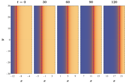
(a)

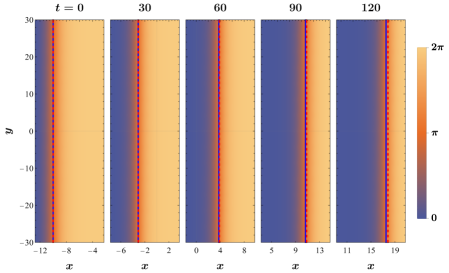
(b)

Figure 1: Comparison of the position of the center of the kink for the results obtained from the full field model and the approximate model. On the left the parameters in the figures shown have values $u=0.025$, $\Gamma=0$ and $\alpha=0$ and on the right $\Gamma=0.003$, $\alpha=0.01$ while velocity is equal to $u_{s}$ according to (2). In both cases $\varepsilon=0$. The dashed red line is the position of the center of the kink according to the approximate model, while the blue line corresponds to the center of the kink from the solution of the full field model.

A slightly different situation is illustrated in Figure 2. The first difference is that the bias current is zero $\Gamma=0$, and so instead of using equation (2) we can choose the initial velocity arbitrarily (here we take $u_{0}=0.2$). The second difference is that the shape of the front is deformed at the initial time. Here we assume the sinusoidal form of the deformation described by the formula

$$X(y,t=0)=X_{0}+\lambda\sin\left(\frac{2\pi y}{L_{y}}\right),$$ (16)

where $L_{y}=60$ is the width of the system along the direction of the $y$ variable. This is selected with the mindset that the any functional form of $X(y,t=0)$ should, in principle, be decomposable in (such) Fourier modes. The value of $X_{0}$ as before is $X_{0}=-20$, while the amplitude of the deformation is $\lambda=0.5$. The value of the dissipation constant in the system is $\alpha=0.001$. As before, there are no inhomogeneities in the system, i.e., $\varepsilon=0$. The method of presenting the results is similar to that used in Figure 1. The left panel illustrates the field configurations obtained from the equation (1), sequentially at instants $t=0,30,60,90,120$. The red solid line represents the kink front at the listed moments of time. On the right panel, the kink positions shown on the left panel (red lines) are compared with those obtained from the effective model (15). The results of the effective model are represented by blue dashed lines. As can be seen, until $t=150$ there are no apparent differences between the results of the field model and the approximate model.

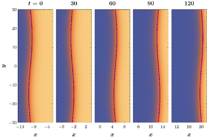
(a)

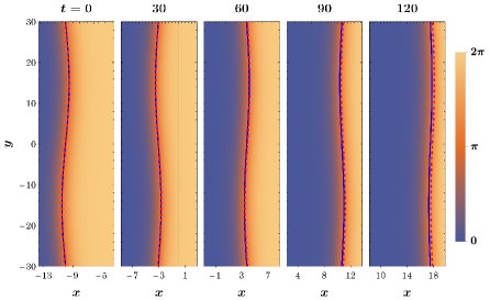
(b)

Figure 2: Comparison of the position of the center of the kink for the results obtained from the full field model and the approximate model with a modification of the initial position of the kink according to equation (16). On the left the parameters in the figures shown have values $u=0.025$, $\Gamma=0$ and $\alpha=0$ and on the right $\Gamma=0.003$, $\alpha=0.01$ and $u_{s}$. In both cases $\varepsilon=0$ and $\lambda=0.5$.

A similar comparison to Figure 2 was made for a more complex shape of the kink initial front. In Figure 3, we studied the case of the initial kink front deformation containing more harmonics

$$X(y,t=0)=X_{0}+\lambda\sum_{n=1}^{N}\sin\left(\frac{2\pi ny}{L_{y}}\right).$$ (17)

In this figure we have shown the evolution of the initial configuration with $N=2$ and $\lambda=0.5$. The other parameters for this case are exactly the same as for the process shown in Figure 2, i.e., among other things, the tested system is homogeneous $\varepsilon=0$ and the kink is not subjected to external force, i.e., $\Gamma=0$. As can be seen in the figure, the correspondence is very good even for $t=150$. An almost identical situation is shown in Figure 4. In the case of this figure, the only difference from Figure 3 is the more complicated form of the kink front, which this time corresponds to $N=3$. In this case, the first noticeable deviations appear for $t=120$.

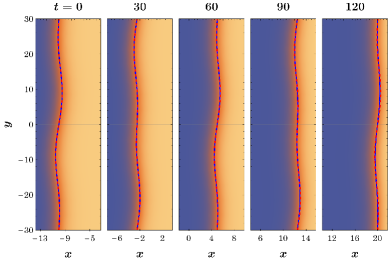
(a)

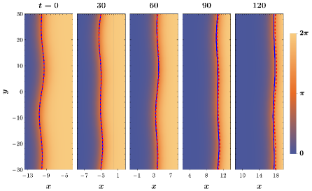
(b)

Figure 3: Comparison of the position of the center of the kink for the results obtained from the full field model and the approximate model with a modification of the initial position of the kink according to equation (17) for $N=2$. On the left the parameters in the figures shown have values $u=0.025$, $\Gamma=0$ and $\alpha=0$ and on the right $\Gamma=0.003$, $\alpha=0.01$ and $u_{s}$. In both cases $\varepsilon=0$ and $\lambda=0.5$.

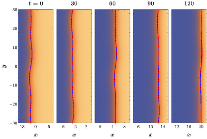
(a)

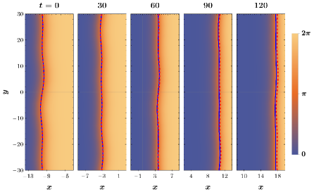
(b)

Figure 4: Comparison of the position of the center of the kink for the results obtained from the full field model and the approximate model with a modification of the initial position of the kink according to equation (17) for $N=3$. On the left the parameters in the figures shown have values $u=0.025$, $\Gamma=0$ and $\alpha=0$ and on the right $\Gamma=0.003$, $\alpha=0.01$ and $u_{s}$. In both cases $\varepsilon=0$ and $\lambda=0.5$.

Summarizing, the simulations shown in the left panels of Figures 2, 3 and 4 demonstrating the evolution of initially deformed kink fronts for $N=1,2,5$ and $\Gamma=0$ were repeated for non-zero bias current. The right panels of these figures show the evolution of the kink front at a bias current equal to $\Gamma=0.003$ and a dissipation coefficient $\alpha=0.01$. In these instances, the initial velocity calculated from equation (2) is $u_{0}=0.229339$. This velocity is the initial condition for the evolution of the kink fronts shown in right panels of Figures 2, 3, 4. Figure 2 according to the formula (17) shows the evolution of a deformed kink front with $N=1$, Figure 3 corresponds to $N=2$, while Figure 4 describes the evolution of a front with $N=5$. In all cases, the front determined on the basis of the approximate equation (15) is slightly delayed compared to the front determined on the basis of the full field equation (1). It turns out that in the first two cases ($N=1$, $N=2$) describing relatively slow deformation of the front (at the initial time), the approximate model gives even for $t=120$ the waveform of the front well reflecting the waveform of the front obtained from the full field model. The situation is slightly different for $N=5$. In this case, quite good agreement is obtained for $t=60$ and even $t=90$, while for $t=120$ we observe small differences.

3.2 Propagation of the front in the presence of an $x$-axis directed inhomogeneity

In this subsection, we will assume that the parameter $\varepsilon$ in equations (1) and (15) is non-zero. Such an assumption means that there is inhomogeneity in the system. In this work, we will describe the effect of inhomogeneity described by the function $g(x,y)=p(x)q(y)$, where $p(x)$ is given by equation (14). In this first introduction of the inhomogeneity, we will assume that $q(y)=1$, which means that the inhomogeneity is in the form of an elevation of height $\varepsilon$, orthogonal to the $x$-direction (which defines the direction of the kink movement). The spatial size of the inhomogeneity along the $x$-direction is approximated by the parameter $h$ appearing in equation (14). In the simulations in this section, we assume $h=10$ and $\varepsilon=0.01$. We study three types of kink dynamics.

In the first case, we consider the a reflection of the kink from a barrier. The course of this process is shown in Figure 5. The case of reflection in the absence of external forcing ($\Gamma=0$) and dissipation ($\alpha=0$) is shown in the left figure. The initial condition in this case is a straight kink front with a velocity $u=0.13$. As in the previous section, the kink front is identified with the line $\phi(t,x,y)=\pi$ (obtained from the field equation (1)). The front is represented by the red line. Regions with $\phi(t,x,y)<\pi$ are once again represented as blue areas, and $\phi(t,x,y)>0$ as yellow. On the other hand, the position of the front determined from equation (15) is represented by the blue dashed line. The gray area represents the position of inhomogeneity. The figure shows the position of the front at instants $t=0,60,120,180$ and $240$. The kink at moments $t=0,60,120$ approaches the inhomogeneity while between moments $t=120$ and $t=180$ it is reflected and turns around, while at instants between $t=180$ and $t=240$ it is already moving towards the initial position. As can be seen, the correspondence of the two descriptions, namely the ones based on equation (1) and on equation (15) is very good, until t=120, while above this value we observe slight deviations. The right figure shows the same process in the case of occurrence of a dissipation $\alpha=0.01$ and forcing $\Gamma=0.00135$ in the system. The course of the front at the same moments as in the left figure also shows very good agreement of the approximate model (15) with the initial model (1), also for t=240. In this figure, the initial velocity of the front is chosen based on the formula (2), i.e., as the stationary velocity. It should be mentioned that the bouncing process in this case is slightly more complex and has an identical (effectively one-dimensional) nature to that described in the one-dimensional case in the paper [45]. It consists of multiple (damped) reflections from the barrier, which eventually ends up stopping before the barrier. As was shown in [45], this reflects the presence of a stable spiral point at such a location which asymptotically attracts the kink towards the relevant fixed point.

In the second case, we are dealing with the interaction of the kink with the inhomogeneity for nearly critical parameter values. This means an initial speed close to the critical velocity in the absence of forcing and dissipation. When dissipation in the system is present and when the forcing is non-zero, then we assume that the forcing takes a value that leads through the formula (2) to a stationary speed approximately equal to the critical velocity. Figure 6, demonstrates this process in detail. The left panel of this figure shows (with labeling identical to this in Figure 5) the interaction of the kink with the inhomogeneity at velocity $u=0.145$. In this case, the kink stays in the inhomogeneity region for a long time. Indeed, by the end of the time frame monitored in Figure 6, the kink has not exited the inhomogeneity. Ultimately, if the time is extended even further then the movement of the kink front to the other side of the inhomogeneity can be observed. The position of the front determined from the field equation (1), with $\alpha=0$ and $\Gamma=0$ is in good coincidence with the position of the kink obtained from the equation (15), up to the time t=120. For longer times slight deviations are observed. On the other hand, the right panel shows results for $\Gamma=0.00155$ and $\alpha=0.01$. It can be seen that, this time as well, the agreement of the position of the front determined from the original equation and the effective one is very good up to the instant t=120. At later moments we observe slight deviations. We would like to underline that Figures show only a part of the space (i.e., from $-18$ to $18$) which in the direction of the $x$-axis is contained in the range from $-70$ to $70$, while in the $y$-axis direction it is contained in the range from $-30$ to $30$.

The last case is shown in Figure 7. The left panel shows the movement of a kink with an initial velocity $u=0.16$ significantly exceeding the critical speed. In this case, slight deviations are already observed for $t=120$. On the other hand, the case with dissipation is presented in the right panel. This figure shows a kink front with an initial speed equal to the stationary velocity determined for dissipation $\alpha=0.01$ and forcing $\Gamma=0.00185$. In this case, the correspondence of the description obtained from equation (1) and equation (15) are striking up to $t=240$. The results obtained in this section are analogous to those described in the paper [45], as the effective motion of the kink is practically one-dimensional and the transverse modulation neither plays a critical role to, nor destabilizes (as is, e.g., the case in nonlinear Schrödinger type models [49]) the longitudinal motion.

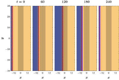
(a)

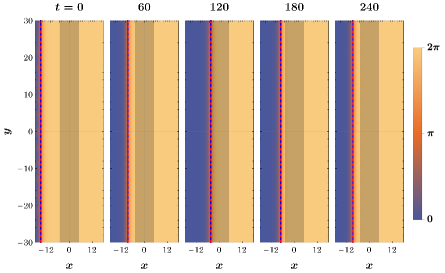
(b)

Figure 5: Comparison of the position of the center of the kink for the results obtained from the full field model and the approximate model. On the left the velocity has value $u=0.13$, and on the right $\Gamma=0.00135$, $\alpha=0.01$ and $u_{s}$. In both cases $\varepsilon=0.01$.

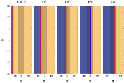
(a)

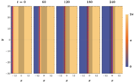
(b)

Figure 6: Comparison of the position of the center of the kink for the results obtained from the full field model and the approximate model. On the left the velocity has value $u=0.145$, and on the right $\Gamma=0.00155$, $\alpha=0.01$ and $u_{s}$. In both cases $\varepsilon=0.01$.

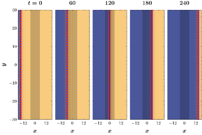
(a)

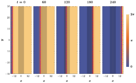
(b)

Figure 7: Comparison of the position of the center of the kink for the results obtained from the full field model and the approximate model. On the left the velocity has value $u=0.16$, and on the right $\Gamma=0.00185$, $\alpha=0.01$ and $u_{s}$. In both cases $\varepsilon=0.01$.

3.3 Kink propagation for inhomogeneities dependent on both variables

In this section we will consider some examples of heterogeneities bearing a genuinely two-dimensional character, i.e., having a non-trivial dependence not only on the $x$-variable initially aligned with the direction of movement of the kink, but also on the $y$ variable, along which the front is initially homogeneous.

3.3.1 Barrier-shaped inhomogeneity

The first example is described by the function $\mathcal{F}(x,y)=1+\varepsilon g(x,y)=1+\varepsilon p(x)q(y)$. The shape of this function is shown in Figure 8. In this case, the function $p(x)$ is given by formula (14) while $q(y)$ has the form:

$$q(y)=\frac{1}{2}\left(\tanh(y+\frac{d}{2})-\tanh(y-\frac{d}{2})\right).$$ (18)

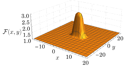
(a)

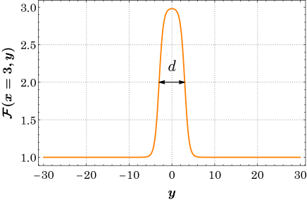
(b)

Figure 8: Left figure presents peak-shaped inhomogeneity $\mathcal{F}(x,y)$, while the right figure shows its section along a line $x=3$. Both parameters $h$ and $d$ are equall to $6$.

We will consider two cases. In the first case, the kink front passes over the inhomogeneity. In the second case, it is stopped by the inhomogeneity. To be more precise, the kink, in the absence of dissipation and forcing, bounces and returns towards its initial position, while when dissipation and forcing are non-zero the kink stops in front of the inhomogeneity due to the emergence of a stable fixed point there. The results of comparing the initial model (1) with the effective model (12) are very good, as can be seen in Figure 9.

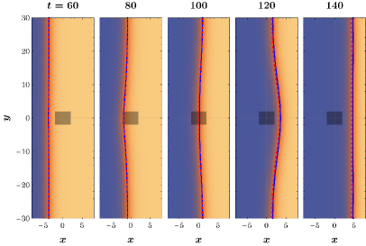
(a)

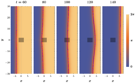
(b)

Figure 9: Passing over heterogeneity. In the left figure, the system without forcing and dissipation. The kink front has an initial velocity equal to $u=0.14$. The right figure shows an analogous process in a system with forcing $\Gamma=0.0018$ and dissipation $\alpha=0.01$. In both images the gray area represents inhomogeneity. Here, we have that $\varepsilon=0.1$. The animations are available through the links https://tinyurl.com/56wwcarr for the left one and https://tinyurl.com/3224zzf7 for the right one.

In the simulations, we assumed a parameter describing the strength of the inhomogeneity equal to $\varepsilon=0.1$. The left panel shows the interaction of the front with the inhomogeneity in the absence of dissipation and forcing. The initial condition in this case is a straight front with a velocity of $u=0.14$. It can be seen that in the course of the evolution the front deforms (the kink bends around the inhomogeneity, which is represented in the figure as a gray area) and then overcomes it. After crossing the inhomogeneity, the tension of the string (the front of the kink) causes it to vibrate, i.e., it excites a transverse mode of the “kink filament”. Obviously, we must remember that local perturbations of the $\phi$-field profile can slightly change the distribution of energy density along the kink front. As a consequence of the existence of tension, the string tends to straighten but excess kinetic energy causes it to vibrate in the direction of the motion of the front, in the absence of dissipation and drive. This oscillation persists for a long time because the mechanism of energy reduction associated with its radiation is not very effective. On the other hand, the right figure shows an analogous process in the case where in the system we have a forcing of $\Gamma=0.0018$ and a dissipation characterized by the coefficient $\alpha=0.01$. In this case, the initial speed is the stationary velocity determined by the formula (2). The course of the process and the results are analogous to the case without dissipation, i.e., we observe local changes in shape that are similar to the left panel. Nevertheless, after passing over the inhomogeneity, we observe damped vibrations that ultimately lead to straightening of the front, as a result of this damped-driven system’s possessing of an attractor (and contrary to the scenario of the conservative Hamiltonian case). The results shown in the figures have also been presented in the form of animations in the associated links. Since in the absence of forcing and dissipation, the mechanism of getting rid of excess energy through radiation is not sufficiently effective, extending the animation time in this case did not lead us to times at which the transverse oscillations of the kink front would disappear. The situation is different when there is dissipation in the system. The animation conducted for long times in the latter setting shows that the kink front straightens.

In the second case, shown in Figure 10, we take a large value of the inhomogeneity strength $\varepsilon=0.5$.

Accordingly, even a front with a velocity slightly greater than the velocity reported in the previous figure is not sufficient to overcome the inhomogeneity. The left panel shows the process of interaction of a front with initial velocity $u=0.16$ with the inhomogeneity represented by the gray area of the figure. As can be seen during the interaction the front is attempting to pass over the inhomogeneity, however, it finally bounces back towards its initial position. Despite the large value of $\varepsilon$, and the substantial deformation of the kink filament, the agreement between the original model (1) and the effective model (12) remains very good. The right panel shows an even more interesting interaction of the kink front with the inhomogeneity. In the figure, in addition to the value of the parameter $\varepsilon=0.5$, a forcing of $\Gamma=0.0013$ and a dissipation coefficient of $\alpha=0.01$ are assumed. Initially the front moving towards the inhomogeneity experiences a deformation. Then, a series of damped reflections of the front from the barrier occur. During the reflections and returns, deformations of the entire front occur having the form of vibrations in the direction of motion. The subsequent turning of the front in the direction of the barrier is a consequence of the existence of an external forcing. Vibrations are damped due to the presence of dissipation in the system. What is interesting here is the final shape of the front, which is a consequence of multiple factors. The first factor is of course, the presence of a barrier that constrains the movement of the front and leads to an energetically induced bending of the kink filament. The second is the presence of forcing, which in the middle is balanced by the presence of the barrier. The situation is different at the ends, where the front does not have “feel” the barrier (and hence is once again straightened). The combination of these factors with the geometric distribution of our inhomogeneity leads to a stable equilibrium analogous to the $1+1$-dimensional case of [45]. Yet, the present case also features a spatial bending of the kink profile, given the geometry of the heterogeneity and the tendency to shorten the length of the kink, in a way resembling the notion of string tension at the front.

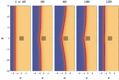
(a)

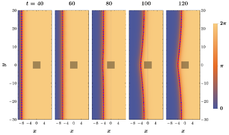
(b)

Figure 10: Reflection/stopping on inhomogeneity. In the left figure, the system without forcing and dissipation is shown. The kink front has an initial velocity equal to $u=0.16$. The right figure shows an analogous process in a system with forcing $\Gamma=0.0013$ and dissipation $\alpha=0.01$. In both pictures, the gray area represents the inhomogeneities with $\varepsilon=0.5$. The animations are available through the links https://tinyurl.com/54u972sb for the left one and https://tinyurl.com/mt6hd9pu for the right one.

3.3.2 Heterogeneity in the form of well.

A slightly different type of inhomogeneity is a potential well. In this section, the well is obtained by replacing $g(x,y)$ in the formula $\mathcal{F}(x,y)=1+\varepsilon g(x,y)=1+\varepsilon p(x)q(y)$ by $-g(x,y)$ and preserving the form of functions $p(x)$ and $q(y)$. In the relevant dip (rather than bump) of the heterogeneity, the parameters are taken as $h=6$ and $d=6$. As in the previous section, we will consider two cases. In the first case, the front passes over the well, and in the second it is stopped by it.

Figure 11 shows the case of a front passing over a well. The left panel describes the case of no forcing and dissipation. The parameter describing the depth of the well is $\varepsilon=0.1$. The initial velocity of the front is $u=0.14$ in this case. A straight front during its approach to the inhomogeneity deforms in the middle part which is related to the attraction by the well (cf. with the opposite scenario of the barrier case explored previously). In the course of crossing the well the situation reverses. Due to the attraction by the inhomogeneity, the central part of the kink advances faster (than the outer parts). Then, we observe the kink moving outside the well, which, in turn, results in vibrations along the direction of motion. These vibrations persist (in the Hamiltonian case) for a very long time due to the lack of dissipation in the system. The right panel shows the same process, but when in the system there is dissipation $\alpha=0.01$ and forcing $\Gamma=0.0018$. The parameter describing the depth of the well is, as before, $\varepsilon=0.1$. The course of the interaction is similar to that in the left panel. The main difference is that the vibration that the front performs after the impact visibly decays and eventually disappears due to the existence of dissipation in the system. Interestingly, in both cases, the agreement of the approximate model with the original one is very good even for long times. As before, we include animations showing the interaction process both in the case without dissipation and with dissipation.

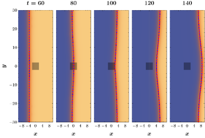
(a)

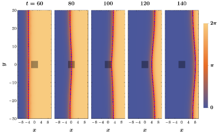
(b)

Figure 11: Passing over the well. In the left figure, the system without forcing and dissipation. The kink front has an initial velocity equal to $u=0.14$. The right figure shows an analogous process in a system with forcing $\Gamma=0.0018$ and dissipation $\alpha=0.01$. In both images the gray area represents the region of inhomogeneity. The parameter describing the depth of the well has a value of $\varepsilon=0.1$. The animations are available through the links https://tinyurl.com/2krhahj6 for the left one and https://tinyurl.com/59p27xps for the right one.

The situation becomes even more interesting in the case shown in Figure 12. In this case, we observe the process of interception of the front by the potential well. The left panel of this figure shows the process of interaction in the absence of forcing and dissipation. The depth of the well here is quite large because it is determined by the parameter $\varepsilon=0.5$. The initial velocity of the kink front is $u=0.16$. As in the previous figure, initially, due to the attraction of heterogeneity, the front in its central part is pulled into the well. Then, there are long-lasting oscillations and deformations of the front, which is the result of interaction with the well. Due to the large value of the parameter $\varepsilon$, the approximation model is less accurate for long times, i.e., ones exceeding $t=100$.

The right panel illustrates an identical process, i.e., interception of the front by the well but with both dissipation ($\alpha=0.01$) and external forcing ($\Gamma=0.0013$) in the system. As in the left panel, the front is initially, in the middle part, pulled into the well and then repeatedly deformed due to interaction with heterogeneity. The important change, once again, is that the deformations of the front, due to dissipation, become gradually smaller. Ultimately, the kink becomes static, adopting a shape different from a straight line, due to the presence of (and attraction to) the heterogeneity. The final shape of the kink is a compromise between the forcing of $\Gamma$ and the tension of the kink filament. Tension, as already mentioned tends to minimize the length of the front while the forcing pushes the free ends of the front to the right. Due to the large value of the $\varepsilon$ parameter, the approximate model has a more limited predictive power for sufficiently long times, e.g., $t>1000$. The discrepancies between the two descriptions seem to have a time shift nature. However, the presence of dissipation leads to a gradual reduction in the kink’s distortion, and thus to the differences between the initial model and the approximate one. It turns out that the final configuration is identical in both models. We have put the course of the impact process in the form of an animations in the additional materials.

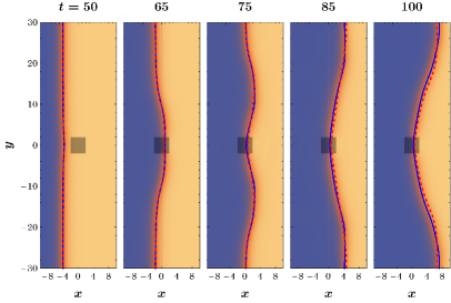
(a)

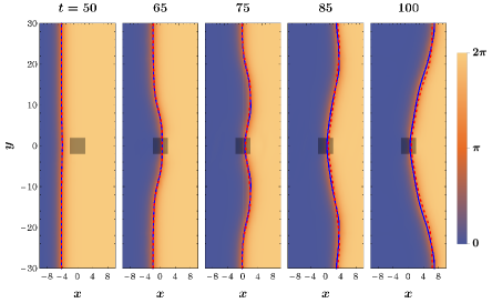
(b)

Figure 12: Intercepting of the kink front through a potential well. On the left, the case without dissipation and forcing is shown. The initial velocity of the front is $u=0.16$. On the right, the dissipation is $\alpha=0.01$ while the forcing is $\Gamma=0.0013$. In both cases, the parameter $\varepsilon$ is equal to $0.5$. The animations are available through the links https://tinyurl.com/2p9h289t for the left one and https://tinyurl.com/y4jxb5sw for the right one.

4 Linear stability of the deformed kink front

In this section we consider the model defined by the equation (1) with $\alpha=0$ and $\Gamma=0$

$$\partial_{t}^{2}\phi-\partial_{x}(\mathcal{F}(x,y)\partial_{x}\phi)-\partial_{y}^{2}\phi+\sin\phi=0.$$ (19)

In the framework of this model we study the stability of the deformed static kink solution $\phi_{0}(x,y)$ satisfying the equation

$$-\partial_{x}(\mathcal{F}(x,y)\partial_{x}\phi_{0})-\partial_{y}^{2}\phi_{0}+\sin\phi_{0}=0.$$ (20)

This study of the spectrum of the kink will help us further elucidate the internal vibrational modes of the kink filament observed and discussed in the previous sections. Indeed, whenever kink vibrations are excited, they can be decomposed on the basis of oscillations of the point spectrum of the kink discussed below (while the extended modes of the continuous spectrum represent the small amplitude radiative wavepackets within the system). Moreover, this spectral analysis can be leveraged to appreciate which configurations are unstable (e.g., the ones where the kink is sitting on top of a barrier) vs. which ones are dynamically stable (e.g., when the kink is trapped by a well).

We introduce into equation (20) a configuration $\phi$ consisting of the solution $\phi_{0}$ and a small correction $\psi$ i.e. $\phi(t,x,y)=\phi_{0}(x,y)+\psi(t,x,y)$. Moreover, we assume a separation of variables of the perturbation in terms of its time and space dependence as: $\psi(t,x,y)=e^{i\omega t}v(x,y).$ In a linear approximation with respect to the correction, we obtain

$$-\partial_{x}\left({\cal F}(x,y)\,\partial_{x}v(x,y)\right)-\partial_{y}^{2}v(x,y)+(\cos\phi_{0})\,v(x,y)=\lambda v(x,y)\,,$$ (21)

where $\lambda=\omega^{2}$. We can briefly write this equation using the $\hat{{\cal L}}$ operator, which includes a dependence on the analytical form of inhomogeneity

$$\hat{{\cal L}}v+\cos\phi_{0}\,v=\lambda v\,.$$ (22)

The above equation has the character of a stationary Schrödinger equation with a potential defined by the cosine of the straight kink front configuration $\phi_{0}$ intercepted by the inhomogeneity. An important feature of this configuration, is that, similarly to the $\hat{{\cal L}}$ operator, it depends in part on the form of the inhomogeneity. In the region of heterogeneity, it has an analytical form different from that of the free kink (denoted $\phi_{K}$ in this work). This modification of the analytical form of the field is a consequence of the interaction of the kink with the inhomogeneity. Based on this equation, an analysis of the excitation spectrum of the static kink captured by the inhomogeneity was carried out. The results can be found in Figures 13 and 14. Figure 13 shows with dotted lines the dependence of the squares of the frequency on the parameter $d$ describing the transverse size of the inhomogeneity. In the figure, the values of the parameters are assumed to be $h=4$ and $\varepsilon=0.1$ (in addition, the size of the system is determined by the values $L_{x}=30$ and $L_{y}=30$). The lowest energy state in this diagram is the non-degenerate state and it corresponds to the zero mode of the sine-Gordon model without inhomogeneities. In addition, the figure includes the fit obtained for this state using an energy landscape study of the one-degree-of-freedom effective model (see Appendix C for a description of this approach). Note that up to a value of about $0.4$ of the $d/L_{y}$ ratio, this simple model captures the course of the numerical dependence well. Above that lie the excited states. At the scale adopted in the figure, it is almost imperceptible that each line actually consists of two lines running side by side. Note that the increase in the value of $\lambda$ for the excited states is similar to the increase in the value for the ground state, as indicated by the dashed lines parallel to the red line obtained for the ground state based on the approximate model (Appendix C). Above a value of unity, we encounter the continuous spectrum of the problem.

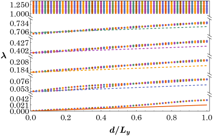
Figure 13: Squared eigenfrequencies $\lambda=\omega^{2}$ calculated for the static kink front configuration (trapped by inhomogeneity with the form of a well) depending on the value of $d/L_{y}$ for $h=4$, $\varepsilon=0.1$. The red line represent the eigenvalue of the ground state obtained from the approximate model described in Appendix C.

A more detailed plot is shown in Figure 14. In this figure, it is much clearer that the discrete states (except for the ground state) are described by double lines. The spectrum is shown here for two values of $\varepsilon$. The results for $\varepsilon=0.01$ are shown in the left figure, while those for $\varepsilon=0.1$ (as in the previous figure) are shown in the right one. The other parameters are identical. The figure also shows the predictions obtained from the degenerate perturbation theory analysis presented in Appendix B. It can be seen that the analytical result reflects very well the course of the line representing the ground state (especially for small values of $\varepsilon$). The course of the lower excited states is also quite well reproduced. For higher excited states, the similarity of the numerical result to the analytical one is qualitative.

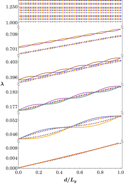
(a)

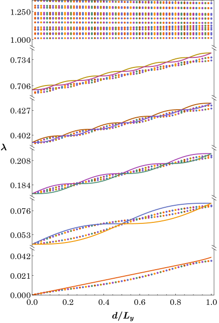
(b)

Figure 14: Detailed graph of squared eigenfrequencies $\lambda=\omega^{2}$ calculated for the static kink configuration trapped by a well (without dissipation and bias current) depending on the value of $d/L_{y}$ for $\varepsilon=0.01$ on the left and $\varepsilon=0.1$ on the right. In both cases $\varepsilon=0.1$, $h=4$. The lines represent the analytical results obtained in Appendix B.

In order to obtain an analytical estimate of the spectrum of linear excitations of the configuration under study, we need, among other things, the form of deformation $\chi$ of the kink front with respect to the free kink. The method of obtaining the $\chi$-function is presented in Appendix A. To check the analytical formulas obtained by approximating, for example, the function $\chi$ in a piecewise form, we performed numerical calculations of the integrals contained in Appendix B based on the approximation (29). The results are presented in figure 15, which was made for the same parameters as figure 14. As can be seen, the improvement in compatibility occurs for the lowest eigenvalues. Specifically, it takes place for the parameter $d/L_{y}$ close to one. For higher eigenvalues, the situation does not significantly improve. It turns out that for higher excited states the analytical formula overestimates the separation of states (corresponding to the degenerate states of the zero approximation), while the result obtained with the fit (29) underestimates this gap. In any event, given the relatively small size of the discrepancy, we do not dwell on this further.

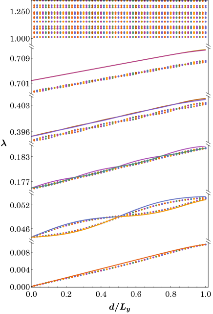
(a)

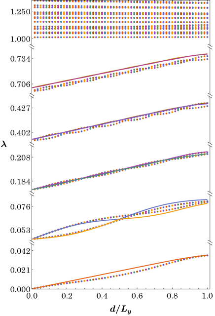
(b)

Figure 15: Detailed graph of squared eigenfrequencies $\lambda=\omega^{2}$ calculated for the static kink configuration trapped by a well (without dissipation and bias current) depending on the value of $d/L_{y}$ for $\varepsilon=0.01$ on the left and $\varepsilon=0.1$ on the right. In both cases $h=4$. The lines represent the results of Appendix B with integrals determined numerically for (29).

On the other hand, the results for a barrier-like inhomogeneity of the form of Figure 8 are presented in Figure 16. The parameters on the left and right panels of this figure are identical and are $h=4$, $\varepsilon=0.1$, $L_{x}=30$, $L_{y}=30$. The figures differ only in scale. This time, the configuration of the kink lying on top of the destabilizing barrier is found to indeed be unstable, which is manifested by the occurrence of a mode with a negative value of $\lambda$ (i.e., an imaginary eigenfrequency). This mode corresponds to the translational mode, reflecting in this case the nature of the effective potential (i.e., a barrier creating an effective saddle point). Such a value is a manifestation of the kink drifting away from inhomogeneity. The other modes are quite similar in nature to the excited modes in the case of potential well, which has its origin in the adopted periodic boundary conditions.

(a)

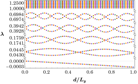
(b)

Figure 16: Squared eigenfrequencies $\lambda=\omega^{2}$ calculated for the static configuration on top of inhomogeneity (without dissipation and bias current) depending on the value of $d/L_{y}$ for $h=4$ and $\varepsilon=0.1$. The left and right figures differ only in scale.

5 Conclusions and Future Challenges

In the current article we studied the behavior of the kink front in the perturbed $2+1$ dimensional sine-Gordon model. The particular type of perturbation is motivated by the study of the dynamics of gauge-invariant phase difference in one- and quasi-one-dimensional curved Josephson junction [29, 20, 21]. We also obtained an effective $1+1$ dimensional model describing the evolution of the kink front based on the non-conservative Lagrangian method [46, 27]. First we tested the usefulness of the approximate model. More concretely, we examined the behavior of the kink starting from the case when there are no inhomogeneities in the system. The agreement between the results of the original and the effective model turned out to be very satisfactory. Subsequently, we explored the movement of the front in a slightly more complex situation. Namely, we examined inhomogeneities of shape independent of the variable transverse to the direction of movement of the front, i.e., the $y$ variable. The results obtained here are in full analogy with the $1+1$ dimensional model studied earlier [45]. These studies can be directly applied to the description of quasi-one-dimensional Josephson junctions.

The most interesting results were obtained for studies of the behavior of the front in the presence of inhomogeneities with shape genuinely dependent on both spatial variables. This case shows the remarkable richness of the dynamical behaviors of the kink front interacting with heterogeneity. We studied two types of inhomogeneities. One was in the form of a barrier, while the other was in the form of a well.

Of particular interest is the process of creating a static final state in the case with dissipation and forcing. We deal with the formation of such a state when a front with too low a velocity is stopped (by a sequence of oscillations) before the peak, and when a front that is too slow is trapped by a well.

We have analyzed the competing factors that contribute to the formation of the resulting stationary states and have shown that our reduced $1+1$-dimensional description can capture the resulting state very accurately. It is worth noting that the approximate description in each of the studied cases is also accurate for long time evolutions for small values of the parameter describing the strength of heterogeneity. While deviations might occur in some cases for very long times (in Hamiltonian perturbations) or for sufficiently large perturbations in dissipative cases, generally, we found that the reduced kink filament model was very accurate in capturing the relevant dynamics.

Finally, we also studied the stability of a straight kink front captured by a single inhomogeneity of the form of a potential well. In this case, the zero mode of the sine-Gordon model without inhomogeneities turns into an oscillating mode in the model with inhomogeneities. Indeed, the breaking of translational invariance leads to either an effective attractive well or a repulsive barrier (see also the analytical justification in Appendix C) manifested in the presence of an internal oscillation or a saddle-like departure from the inhomogeneous region. In addition, the periodic boundary conditions we have adopted result in a number of additional discrete modes appearing in the system in addition to the ground state and the continuous spectrum. These are effectively the linear modes associated with the quantized wavenumbers due to the transverse domain size. In the absence of a genuinely 2d heterogeneity, this picture can be made precise with the respective eigenmodes being $k_{y}=2n\pi/L_{y}$. In the presence of genuinely $2$d heterogeneities, the picture is still qualitatively valid, but the modes are locally deformed and then a degenerate perturbation theory analysis is warranted, as shown in Appendix B, where we have provided such an analytical description of the mode structure This description matches quite well with the numerical results - especially for the lower states of the spectrum under study.

Naturally, there are numerous extensions of the present work that are worth exploring in the future. More specifically, in the present setting we have focused on inhomogeneities impacted upon by rectilinear kink structures, while numerous earlier works [37, 38, 40, 30] have considered the interesting additional effects of curvature in the two-dimensional setting. In light of the latter, it would be interesting to examine heterogeneities in such radial cases. Furthermore, in the sine-Gordon case, the absence of an internal mode in the quasi-one-dimensional setting may have a significant bearing of a phenomenology and the possibility of energy transfer type effects that occur, e.g., in the $\phi^{4}$ model [50]. It would, thus, be particularly relevant to explore how the relevant phenomenology generalizes (or is modified) in the latter setting. Finally, while two-dimensional settings have yet to be exhausted (including about the potential of radial long-lived breathing-like states), it would naturally also of interest to explore similar phenomena in the three-dimensional setting. Such studies are presently under consideration and will be reported in future publications.

6 Appendix A

6.1 Peak-shaped inhomogeneity

We will consider the case of a kink front stopped by the inhomogeneity (in the form of a barrier; see Fig. 8) in the presence of forcing and dissipation. The static configuration in this case is the solution of the following equation

$$-\partial_{x}(\mathcal{F}(x,y)\partial_{x}\phi_{0})-\partial_{y}^{2}\phi_{0}+\sin\phi_{0}=-\Gamma.$$ (23)

To begin with, we will show that the solution can be represented (for small perturbations) as the sum of a kink profile $\phi_{K}=4\arctan e^{x-X_{0}(y)}$ and a correction that depends only on the shape of the inhomogeneity and the external forcing i.e. $\phi_{0}(x,y)=\phi_{K}(x-X_{0})+\chi(x,y).$ The equation satisfied by the correction $\chi$, to leading order,is of the form

$$-\partial_{x}\left({\cal F}(x,y)\partial_{x}\chi\right)-\partial_{y}^{2}\chi+(\cos\phi_{K}(x-X_{0}))\chi=\varepsilon\partial_{x}\left(g(x,y)\partial\phi_{K}(x-X_{0})\right)-\Gamma.$$ (24)

The results of simulations performed on the ground of approximation (24) and the field model (23) are demonstrated in Figure 17. This figure shows in the left panel the $\chi$ profiles obtained for different values of the $\varepsilon$ parameter. Starting from the top, we have $\varepsilon=0.1$, $\varepsilon=0.2$ and $\varepsilon=0.5$. In all cases, $\Gamma=0.001$. The right panel shows the profile of the static kink front in the same cases. This panel, on the one hand, shows the static kink front obtained from equation (23) (black dashed line), and on the other hand, the fronts obtained from the solutions of equation (24) for different values of the parameter $\varepsilon$. The red line corresponds to $\varepsilon=0.1$, the blue line corresponds to $\varepsilon=0.2$, while the yellow line corresponds to $\varepsilon=0.5$. These fronts were determined for the $\phi_{K}+\chi$ configuration. The deformation of the kink center is due to the fact that it is supported by the inhomogeneity in the central part, and on the other hand, at the edges it is stretched by the existing constant forcing. Of course, due to the tension of the kink front, stretching cannot take place unrestrictedly because this would lead to an excessive increase in the total energy stored in the kink configuration. Let us notice that in all cases, qualitatively the shape of the static kink front is correctly reproduced. On the other hand, in the case of $\varepsilon=0.5$ we observe some quantitative deviations in the central part.

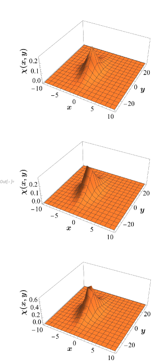
(a)

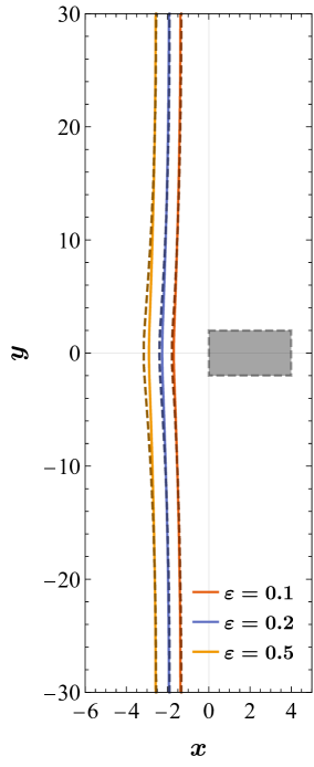
(b)

Figure 17: The left panel shows the function $\chi(x,y)$ for, starting from top, $\varepsilon=0.1,0.2$ and $0.5$. The right figure compares the shape of the kink front obtained using the equation (24) with the exact results represented by the dashed black line, for the same values of $\varepsilon$. The forcing is assumed here to be $\Gamma=0.001$.

We also test the stability of the above described solution is based on the equation which looks identical to the equation (21), however, the main difference is the relationship of the eigenvalue $\lambda$ to the frequency. In the case considered in this section $\lambda=\omega(\omega-i\alpha)$. Figure 18 shows the dependence of the square of the frequency $\omega$ on the parameter $d/L_{y}$. It can be seen that the excitation spectrum determined for the configuration shown in Figure 17, consists of a ground state, excited states and a continuous spectrum. The form of this spectrum is to a significant degree similar to the excitation spectrum of the kink front trapped by the potential well, and shown in Figures 14, 15. The main difference from the previous diagrams is that the discrete excited states show less periodicity as in the previous figures.

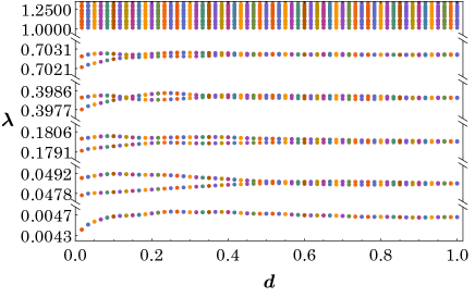
Figure 18: Graph of squared eigenfrequencies $\omega^{2}$ calculated for the static kink configuration stopped by a barrier (with dissipation and bias current) depending on the value of $d/L_{y}$ for $\varepsilon=0.5$ and $h=4$.

6.2 Heterogeneity with a form of well

In this section, we describe the change in the profile of the static kink that results from the existence of an inhomogeneity in the form of a well. We assume that the well is centrally located and has dimensions defined by the parameters $h$ and $d$ i.e. ${\cal F}(x,y)=1+\varepsilon g(x,y)=1-\varepsilon p(x)q(y)$ and

$$p(x)=\frac{1}{2}\left[\tanh\left(x+\frac{h}{2}\right)-\tanh\left(x-\frac{h}{2}\right)\right]\approx\begin{cases}1,&x\in[-\frac{h}{2},+\frac{h}{2}]\\ 0,&x\notin[-\frac{h}{2},+\frac{h}{2}]\end{cases},$$ (25)

$$q(y)=\frac{1}{2}\left[\tanh\left(y+\frac{d}{2}\right)-\tanh\left(y-\frac{d}{2}\right)\right]\approx\begin{cases}1,&y\in[-\frac{d}{2},+\frac{d}{2}]\\ 0,&y\notin[-\frac{d}{2},+\frac{d}{2}]\end{cases}.$$ (26)

The approximate form used to calculate some integrals when determining the analytical form of the eigenvalues (see Appendix B) is also given in the above expression. An example profile obtained from equation (24) in the absence of bias current ($\Gamma=0$) is shown in Figure 19. The shape of the $\chi$ function, although shown for specific parameter values (i.e., $h=4$, $d=4$ and $\varepsilon=0.1$), is characteristic over a wide range of parameters. The profile shown in Figures 20 is an even function in the $y$ variable and an odd function in the $x$ variable.

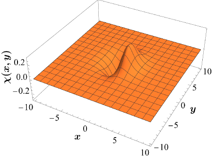
Figure 19: The shape of the function $\chi(x,y)$, for a static kink front trapped by a well-shaped inhomogeneity. The parameters in the figure are as follows: $d=4$, $h=4$, $\varepsilon=0.1$.

The panels of figure 20 also include a simple fit in the form of the step function. The parameter $\chi_{0}$ was chosen so that the areas under the curves $\alpha=\alpha(x)$, $\beta=\beta(y)$ and the fit were identical.

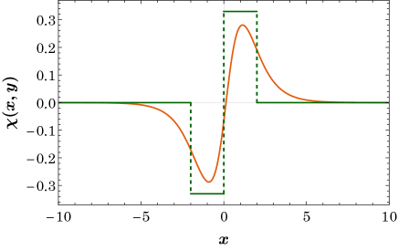
(a)

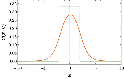
(b)

Figure 20: Cross sections with fitting for $\chi(x,y)$. The value of $\chi_{0}=0.67$ was determined by fit. Here $h=4$, $d=4$ and $\varepsilon=0.1$.

In the next section (appendix B), we use this form of the $\chi$ function to approximate the eigenvalues when studying the stability of a static configuration trapped by a well-like inhomogeneity

$$\chi(x,y)=\chi_{0}\,\,\alpha(x)\beta(y),$$ (27)

$$\alpha(x)\approx\begin{cases}-1,&x\in[-\frac{h}{2},0)\\ +1,&x\in[0,+\frac{h}{2}]\\ 0,&\text{otherwise}\end{cases},\;\;\;\;\beta(y)\approx\begin{cases}+1,&x\in[\frac{d}{2},+\frac{d}{2}]\\ 0,&\text{otherwise}\end{cases}\,\,\,.$$ (28)

In order to validate the analytical expressions (47) and (61) for the eigenvalues of the linear excitation operator, we also determined a much better fit for the $\chi$ function. We looked for the fit in the form:

$$\chi(x,y)=\chi_{0}\tanh(ax)\operatorname{sech}(ax)\left(4\arctan e^{y+\frac{d}{2}}-4\arctan e^{y-\frac{d}{2}}\right).$$ (29)

The shape of the fit was compared with the numerical result. The example figure 21 shows a very good convergence between the fit (dashed line) and the numerical result (solid line). The figure was made for parameters equal to $\chi_{0}=0.67$, $a=0.85$, $h=4$, respectively. The fit form described by equation (29) was also used to determine the numerical value of the integrals in Appendix B. The results obtained on this basis are presented in Figure 15. As can be seen for lower eigenvalues, we observe improved agreement with numerical results. Moreover, the improvement is evident for values of $d/L_{y}$ close to one.

(a)

(b)

Figure 21: Cross sections with fitting for $\chi(x,y)$. The dashed green line represents a fit function of the form $\chi(x,y)=\chi_{0}\tanh(ax)\operatorname{sech}(ax)\left(4\arctan e^{y+\frac{d}{2}}-4\arctan e^{y-\frac{d}{2}}\right)$. Here $h=4$, $d=10$ and $\varepsilon=0.1$.

7 Appendix B - Kink stability in the potential well

In this section, we will present analytical results on the spectrum of linear excitations of a deformed kink bounded by an inhomogeneity in the form of a potential well. We start with the equation (22)

$$\hat{{\cal L}}v+\cos\phi_{0}\,v=\lambda v\,.$$ (30)

Since we plan to use perturbation calculus in the parameter $\varepsilon$ determining the magnitude of the inhomogeneity, we separate the operator $\hat{{\cal L}}$ into a part $\hat{{\cal L}_{0}}$ that does not depend on the perturbation parameter and a part $\hat{W}$ preceded by this parameter. The relationships between operators and the other quantities used in this section are summarized below

$$\hat{{\cal L}}v=\hat{{\cal L}_{0}}v+\varepsilon\hat{W}v,\,\,\,\,\,\,\hat{{\cal L}_{0}}v=-\partial_{x}^{2}v-\partial_{y}^{2}v,\,\,\,\,\,\,\hat{W}v=-\partial_{x}\left(g(x,y)\,\partial_{x}v\right),\,\,\,\,\,\,{\cal F}(x,y)=1+\varepsilon g(x,y).$$ (31)

According to the results presented in appendix A, we can separate the static kink configuration in the presence of inhomogeneity into static free kink $\phi_{K}$ and deformation associated with the existence of inhomogeneity $\chi$

$$\phi_{0}(x,y)=\phi_{K}(x)+\chi(x,y).$$ (32)

Next, we expand the quantities appearing in formula (30) with respect to the parameter $\varepsilon$

$$v=v^{(0)}+\varepsilon v^{(1)}+\varepsilon^{2}v^{(2)}+...$$ (33)

$$\lambda=\lambda^{(0)}+\varepsilon\lambda^{(1)}+\varepsilon^{2}\lambda^{(2)}+...,$$ (34)

$$\chi=\chi^{(0)}+\varepsilon\chi^{(1)}+\varepsilon^{2}\chi^{(2)}+....$$

The function $\chi$ is defined in such a way that it does not appear in the zero order, i.e. $\chi^{(0)}=0$. In addition, since in the system under consideration we assume periodic boundary conditions in the direction of the $y$ variable we also take $v(x,-\frac{1}{2}L_{y})=v(x,+\frac{1}{2}L_{y}).$ Moreover, it is assumed that the inhomogeneity disappears at the edges of the system (in the direction of the variable $x$), i.e. $g(x,y)\rightarrow 0$ for $x\rightarrow\pm\frac{1}{2}L_{x}.$ Note also that, like $\partial_{x}\phi(\pm\frac{1}{2}L_{x},y)$, also $\partial_{x}v(\pm\frac{1}{2}L_{x},y)$ disappears at the $x$ boundaries of the area under consideration.

7.1 The lowest order of expansion

In the lowest order, we get the equation

$$\hat{{\cal L}_{0}}v^{(0)}+\cos\phi_{K}\,v^{(0)}=\lambda^{(0)}v^{(0)}\,,$$ (35)

where $\phi_{K}(x)=4\arctan(e^{x})$ describes the kink front located at $x=0$ and stretched along the $y$-axis. For the function $\phi_{K}(x)$, the equation can be separated into two equations. One depending on the $x$ variable and the other on $y$. Using periodicity in the $y$ variable, we obtain a series of eigenvalues and eigenfunctions. The ground state in this approximation corresponds to zero eigenvalue

$$\lambda^{(0)}_{0}=0,\,\,\,\,\,v^{(0)}_{0}(x,y)=A_{0}\,\mathrm{sech}(x),\,\,\,\,\,A_{0}=\frac{1}{\sqrt{2L_{y}\tanh\frac{L_{x}}{2}}}.$$ (36)

The subsequent eigenstates correspond to non-zero eigenvalues

$$\lambda^{(0)}_{n\pm}=\left(\frac{2\pi}{L_{y}}\right)^{2}n^{2},\,\,\,\,\,\,\,\begin{cases}v^{(0)}_{n+}(x,y)=A\,\mathrm{sech}(x)\cos(2\pi n\frac{y}{L_{y}})\\ v^{(0)}_{n-}(x,y)=A\,\mathrm{sech}(x)\sin(2\pi n\frac{y}{L_{y}})\end{cases},\,\,\,\,\,\,A=\frac{1}{\sqrt{L_{y}\tanh\frac{L_{x}}{2}}}.$$ (37)

In the lowest order of the perturbation calculus, all non-zero eigenvalues are degenerate twice. The normalization coefficients $A$ and $A_{0}$ were chosen so that the eigenfunctions were normalized to one in the sense of the product defined as the integral over the area $[-L_{x}/2,+L_{x}/2]\times[-L_{y}/2,+L_{y}/2]$, according to the formula

$$\langle u,v\rangle\equiv\int_{-\frac{L_{x}}{2}}^{+\frac{L_{x}}{2}}\int_{-\frac{L_{y}}{2}}^{+\frac{L_{y}}{2}}u(x,y)v(x,y)dxdy,$$ (38)

where we assume that functions are periodic with respect to the variable $y$ and their $x$-derivatives disappear at the boundaries $x=\pm\frac{L_{x}}{2}$ .

7.2 The first order of expansion

In the first-order of expansion the equation is of the form

$$\hat{{\cal L}_{0}}v^{(1)}+\cos\phi_{K}\,v^{(1)}+\hat{G}v^{(0)}=\lambda^{(0)}v^{(1)}+\lambda^{(1)}v^{(0)}\,.$$ (39)

In order to shorten the formulas that appear in this section, the operator $\hat{G}$ was introduced

$$\hat{G}v^{(0)}\equiv\hat{W}v^{(0)}-(\sin\phi_{K})\chi^{(1)}v^{(0)}.$$ (40)

7.2.1 Correction to the ground state

We project equation (39) for the ground state onto the state $v_{0}^{(0)}$ which leads to the equation

$$\langle v_{0}^{(0)},(\hat{{\cal L}_{0}}+\cos\phi_{K})\,v_{0}^{(1)}\rangle+\langle v_{0}^{(0)},\hat{G}v_{0}^{(0)}\rangle=\lambda^{(0)}_{0}\langle v_{0}^{(0)},v_{0}^{(1)}\rangle+\lambda^{(1)}_{0}\langle v_{0}^{(0)},v_{0}^{(0)}\rangle\,.$$ (41)

Due to the normalization of the state $v_{0}^{(0)}$ and the fact that the operator $\hat{{\cal L}_{0}}+\cos\phi_{K}$ is hermitian, i.e.,

$$\langle v,(\hat{{\cal L}_{0}}+\cos\phi_{K})\,u\rangle=\langle(\hat{{\cal L}_{0}}+\cos\phi_{K})v,u\rangle\,,$$ (42)

equation (41) can be reduced to the form

$$\lambda_{0}^{(1)}=\langle v_{0}^{(0)},\hat{G}v_{0}^{(0)}\rangle.$$ (43)

We determine the value of $\lambda_{0}^{(1)}$ based on equations (40) and (31). In the appendix, we take the following form of $g(x,y)=-p(x)q(y)$. As for the function describing the deformation of the function $\phi_{0}$ resulting from the existence of inhomogeneities, i.e., $\chi^{(1)}$, we write it as follows $\chi^{(1)}=\chi_{0}\,\,\alpha(x)\beta(y)$. Under the above conditions, the correction of first order is of the form

$$\lambda_{0}^{(1)}=\frac{1}{2L_{y}\tanh\frac{L_{x}}{2}}\left(2\chi_{0}J_{\alpha}I_{\beta}-J_{p}I_{q}\right).$$ (44)

The integrals that appear in the above formula are defined below

$$J_{p}\equiv\int^{+\frac{L_{x}}{2}}_{-\frac{L_{x}}{2}}p(x)~{}\mathrm{sech}^{2}(x)\tanh^{2}(x)~{},\,\,\,\,\,\,I_{q}\equiv\int^{+\frac{L_{y}}{2}}_{-\frac{L_{y}}{2}}q(y)dy,$$ (45)

$$J_{\alpha}\equiv\int^{+\frac{L_{x}}{2}}_{-\frac{L_{x}}{2}}\alpha(x)~{}\mathrm{sech}^{3}(x)\tanh(x)~{},\,\,\,\,\,\,I_{\beta}\equiv\int^{+\frac{L_{y}}{2}}_{-\frac{L_{y}}{2}}\beta(y)dy.$$ (46)

The $p(x)$ and $q(x)$ functions appearing in the above integrals, in the paper, are taken in the form of (25) and (26). On the other hand, the form of the function $\chi(x,y)\approx\chi^{(1)}(x,y)$ is approximated, according to considerations contained in appendix A in formulas (28). Two of the above integrals approximately describe the width of the inhomogeneity in the direction of the $y$ variable i.e. $I_{q}\approx d$ , $I_{\beta}\approx d.$ Consequently, the eigenvalue of the ground state takes the form of

$$\lambda_{0}=\lambda_{0}^{(0)}+\varepsilon\lambda_{0}^{(1)}+...\approx\frac{\varepsilon}{2\tanh\frac{L_{x}}{2}}~{}\frac{d}{L_{y}}~{}\left(2\chi_{0}J_{\alpha}-J_{p}\right).$$ (47)

To complete the result obtained, we provide the integrals appearing in this formula

$$J_{\alpha}\approx\frac{2}{3}\left(1-\mathrm{sech}^{3}\left(\frac{h}{2}\right)\right),$$ (48)

$$J_{p}=\coth\left(\frac{h}{2}\right)\left[\frac{2\tanh\left(\frac{L_{x}}{2}\right)-\coth\left(\frac{h}{2}\right)~{}\ln\left(\frac{\cosh\left(\frac{L_{x}+h}{2}\right)}{\cosh\left(\frac{L_{x}-h}{2}\right)}\right)}{\sinh^{2}\left(\frac{h}{2}\right)}+\frac{2}{3}\tanh^{3}\left(\frac{L_{x}}{2}\right)\right].$$ (49)

7.2.2 Correction to the degenerate states

In the case of degenerate states, we perform a projection of equation (39) into a state that is a combination of zero-order eigenstates

$$v_{n}=\sum_{i=\pm}c_{i}v^{(0)}_{ni}.$$ (50)

Projection of the equation of the first order written for the degenerate state $v_{nj}^{0}$ onto the $v$ state gives

$$\langle v_{n},(\hat{{\cal L}_{0}}+\cos\phi_{K})\,v_{nj}^{(1)}\rangle+\langle v_{n},\hat{G}v_{nj}^{(0)}\rangle=\lambda^{(0)}_{n}\langle v_{n},v_{nj}^{(1)}\rangle+\lambda^{(1)}_{n}\langle v_{n},v_{nj}^{(0)}\rangle\,.$$ (51)

Orthonormality of the zero-order states and hermiticity of the operator $\hat{{\cal L}_{0}}+\cos\phi_{K}$ leads to a system of equations for the coefficients $c_{i}$

$$\sum_{i=\pm}c_{i}\langle v^{(0)}_{ni},\hat{G}v^{(0)}_{nj}~{}\rangle=\lambda^{(1)}_{n}\sum_{i=\pm}c_{i}~{}\delta_{ij}.$$ (52)

Due to the second degree of degeneracy, we can write the last equation in $2\times 2$ matrix form

$$\left[\begin{array}[]{cc}G_{++}-\lambda^{(1)}_{n}&G_{+-}\\ G_{-+}&G_{++}-\lambda^{(1)}_{n}\\ \end{array}\right]\Biggl{[}\begin{array}[]{c}c_{+}\\ c_{-}\\ \end{array}\Biggr{]}=\Biggl{[}\begin{array}[]{c}0\\ 0\\ \end{array}\Biggr{]},$$ (53)

where the matrix elements $G_{ij}$ are written in the basis that consists of eigenstates of the zero order approximation

$$G_{ij}=\langle v^{(0)}_{ni},\hat{G}v^{(0)}_{nj}~{}\rangle.$$ (54)

The condition for the existence of non-trivial solutions of the above equation is the zeroing of the determinant (so that nontrivial solutions of the homogeneous system exist)

$$\left|\begin{array}[]{cc}G_{++}-\lambda^{(1)}_{n}&G_{+-}\\ G_{-+}&G_{++}-\lambda^{(1)}_{n}\\ \end{array}\right|=0.$$ (55)

According to the above equation, corrections of the first order remove the degeneracy, leading to the eigenvalue corrections:

$$\lambda^{(1)}_{n\pm}=\frac{1}{2}\left[~{}(G_{++}+G_{--})\pm\sqrt{(G_{++}-G_{--})^{2}+4G_{+-}G_{-+}}~{}\right].$$ (56)

The expression above is greatly simplified due to the evenness of the $q(-y)=q(y)$ and $\beta(-y)=\beta(y)$ functions in the $y$ variable. This property removes the matrix element $G_{+-}=0$ which leads to a significant simplification of the last formula

$$\lambda^{(1)}_{n\pm}=\frac{1}{2}\left[~{}(G_{++}+G_{--})\pm|G_{++}-G_{--}|~{}\right].$$ (57)

Matrix elements that appear in the above expression

$$G_{++}=A^{2}\left(2\chi_{0}~{}J_{\alpha}I^{+}_{\beta}-J_{p}I^{+}_{q}~{}\right),\,\,\,\,\,\,G_{--}=A^{2}\left(2\chi_{0}~{}J_{\alpha}I^{-}_{\beta}-J_{p}I^{-}_{q}~{}\right),$$ (58)

are written using integrals

$$I_{q}^{+}=\int_{-\frac{L_{y}}{2}}^{+\frac{L_{y}}{2}}q(y)\cos^{2}\left(2\pi n\frac{y}{L_{y}}\right)dy,\,\,\,\,I_{q}^{-}=\int_{-\frac{L_{y}}{2}}^{+\frac{L_{y}}{2}}q(y)\sin^{2}\left(2\pi n\frac{y}{L_{y}}\right)dy,$$ (59)

$$I_{\beta}^{+}=\int_{-\frac{L_{y}}{2}}^{+\frac{L_{y}}{2}}\beta(y)\cos^{2}\left(2\pi n\frac{y}{L_{y}}\right)dy,\,\,\,\,I_{\beta}^{-}=\int_{-\frac{L_{y}}{2}}^{+\frac{L_{y}}{2}}\beta(y)\sin^{2}\left(2\pi n\frac{y}{L_{y}}\right)dy.$$ (60)

The final result shows the disappearance of the degeneracy of the higher eigenvalues (the integrals $J_{\alpha}$ and $J_{p}$ are defined by the formulas (48) and (49))

$$\lambda_{n\pm}=\lambda^{(0)}_{n}+\varepsilon\lambda^{(1)}_{n\pm}+...\approx\left(\frac{2\pi}{L_{y}}\right)^{2}n^{2}+\frac{\varepsilon}{2\tanh\left(\frac{L_{x}}{2}\right)}~{}(2\chi_{0}~{}J_{\alpha}-J_{p})\left[\frac{d}{L_{y}}\pm\left|\frac{\sin\left(2\pi n\frac{d}{L_{y}}\right)}{2\pi n}\right|~{}\right].$$ (61)

This result was obtained by means of the approximation:

$$I_{q}^{\pm}\approx\frac{1}{2}~{}L_{y}\left(\frac{d}{L_{y}}\pm\frac{\sin\left(2\pi n\frac{d}{L_{y}}\right)}{2\pi n}\right),\,\,\,\,I_{\beta}^{\pm}\approx\frac{1}{2}~{}L_{y}\left(\frac{d}{L_{y}}\pm\frac{\sin\left(2\pi n\frac{d}{L_{y}}\right)}{2\pi n}\right).$$ (62)

In addition, the normalization factor $A$ included in formula (37) was used, while the values of the integrals $J_{\alpha}$ and $J_{p}$ are defined by the formulas (48) and (49).

8 Appendix C

In this section, we will estimate the value of $\lambda=\omega^{2}$ corresponding to the ground state, based on the shape of the energy landscape of the system under study. We consider the Lagrangian density of the sine-Gordon model in the presence of inhomogeneity

$${\cal L}=\frac{1}{2}(\partial_{t}\phi)^{2}-\frac{1}{2}{\cal F}(x,y)(\partial_{x}\phi)^{2}-\frac{1}{2}(\partial_{y}\phi)^{2}-V(\phi).$$ (63)

The energy density in this model is of the form

$$\rho=\frac{1}{2}(\partial_{t}\phi)^{2}+\frac{1}{2}{\cal F}(x,y)(\partial_{x}\phi)^{2}+\frac{1}{2}(\partial_{y}\phi)^{2}+V(\phi).$$ (64)

As in previous parts $V(\phi)=1-\cos\phi$ and ${\cal F}(x,y)=1+\varepsilon g(x,y).$ Into the expression for the energy density we insert the kink ansatz $\phi_{K}(t,x)=4\arctan e^{x-x_{0}(t)}$, where $x_{0}=x_{0}(t)$ determines the position of the kink. Based on expression (64), we calculate the energy per unit length of the kink front

$$E(x_{0})=\frac{1}{L_{y}}\int_{-\frac{L_{x}}{2}}^{+\frac{L_{x}}{2}}\int_{-\frac{L_{y}}{2}}^{+\frac{L_{y}}{2}}\rho(x,y,x_{0})dxdy=\frac{1}{2}m\dot{x_{0}}^{2}+\widetilde{V}(x_{0}).$$ (65)

The first term has its origin in the differentiation of the kink ansatz with respect to the time variable $\partial_{t}\phi_{K}=-\dot{x_{0}}\,\partial_{x}\phi_{K}$ and $m=8\tanh{\frac{L_{x}}{2}}\approx 8$ is the mass of a free, resting kink (where $L_{x}=30$). The next terms define the potential energy. Under the assumption as to the form of inhomogeneity $g(x,y)=-p(x)q(y)$, the potential energy can be expressed by two integrals

$$\widetilde{V}(x_{0})=8-2\varepsilon I(d)J(x_{0},h),$$ (66)

where we denoted

$$I(d)=\frac{1}{Ly}\int_{-\frac{L_{y}}{2}}^{+\frac{L_{y}}{2}}q(y)dy=\frac{1}{L_{y}}\ln\left(\frac{\cosh\left(\frac{L_{y}+d}{2}\right)}{\cosh\left(\frac{L_{y}-d}{2}\right)}\right)\approx\frac{d}{L_{y}},\,\,\,\,\,\,J(x_{0},h)=\int_{-\frac{L_{x}}{2}}^{+\frac{L_{x}}{2}}p(x)\operatorname{sech}^{2}(x-x_{0})dx.$$ (67)

For a more compact result (and because of the rapid disappearance of the $p$-function when approaching the edge), we approximate the second integral as follows

$$J(x_{0},h)\approx\int_{-\infty}^{+\infty}p(x)\operatorname{sech}^{2}(x-x_{0})dx=-\left(\frac{2x_{0}+h-\sinh(2x_{0}+h)}{\cosh(2x_{0}+h)-1}-\frac{2x_{0}-h-\sinh(2x_{0}-h)}{\cosh(2x_{0}-h)-1}\right).$$ (68)

In the vicinity of the center of the well (i.e., for $x_{0}=0$), we can approximate the potential energy (66) to the accuracy of the harmonic term

$$\widetilde{V}(x_{0})\approx A+Bx_{0}^{2},$$ (69)

where the expansion coefficients are respectively

$$A=8+4\varepsilon\frac{d}{L_{y}}\,\left(\frac{h-\sinh h}{\cosh h-1}\right)\,\,,\,\,\,\,\,B=2\varepsilon\frac{d}{L_{y}}\,\mathrm{csch}^{4}\left(\frac{h}{2}\right)\,\left[h(2+\cosh h)-3\sinh h\right].$$ (70)

We can rescale the original potential $\widetilde{V}(x_{0})$ by a constant getting a new potential $V(x_{0})=\widetilde{V}(x_{0})-A$. The effective Lagrangian for this system is thus of the form

$$L=\frac{1}{2}m\dot{x_{0}}^{2}-Bx_{0}^{2}.$$ (71)

The effective equation is that of a harmonic oscillator

$$\ddot{x}_{0}+\frac{2B}{m}x_{0}=0.$$ (72)

The eigenfrequency of this oscillator describes, in a manner independent of the perturbation calculus performed in Appendix B (i.e., the latter is at the level of the equation of motion, while here we work at the level of the corresponding Lagrangian and energy functionals), the ground state appearing in the description of the linear stability of a kink trapped by a well-shaped inhomogeneity.

$$\omega^{2}=\frac{2B}{m}=\frac{1}{2}\varepsilon\frac{d}{L_{y}}\,\mathrm{csch}^{4}\left(\frac{h}{2}\right)\,\left[h(2+\cosh h)-3\sinh h\right].$$ (73)

The relevant results is showcased in Fig. 13.

References

- [1] J. Frenkel and T. Kontorova “On the theory of plastic deformation and twinning” In J. Phys. Acad. Sci. USSR 1, 1939, pp. 137
- [2] Vadim Zharnitsky, Igor Mitkov and Mark Levi “Parametrically forced sine-Gordon equation and domain wall dynamics in ferromagnets” In Phys. Rev. B 57 American Physical Society, 1998, pp. 5033–5035 DOI: 10.1103/PhysRevB.57.5033
- [3] S. Bugaychuk et al. “Wave-mixing solitons in ferroelectric crystals” In Radiation Effects and Defects in Solids 157.6-12 Taylor & Francis, 2002, pp. 995–1001 DOI: 10.1080/10420150215749
- [4] L. Lam “Solitons in Liquid Crystals” New York, NY: Springer New York, 1992, pp. 9–50 DOI: 10.1007/978-1-4612-0917-1˙2
- [5] B.D. Josephson “Possible new effects in superconductive tunnelling” In Physics Letters 1.7, 1962, pp. 251–253 DOI: https://doi.org/10.1016/0031-9163(62)91369-0
- [6] Aihua Xie, Lex Meer, Wouter Hoff and Robert H. Austin “Long-Lived Amide I Vibrational Modes in Myoglobin” In Phys. Rev. Lett. 84 American Physical Society, 2000, pp. 5435–5438 DOI: 10.1103/PhysRevLett.84.5435
- [7] Danko Georgiev, Stelios Papaioanou and James Glazebrook “Neuronic system inside neurons: molecular biology and biophysics of neuronal microtubules” In Biomedical Reviews 15.0, 2004 URL: https://journals.mu-varna.bg/index.php/bmr/article/view/103
- [8] Niels R Walet and Wojtek J Zakrzewski “A simple model of the charge transfer in DNA-like substances” In Nonlinearity 18.6, 2005, pp. 2615 DOI: 10.1088/0951-7715/18/6/011
- [9] J. Bednář “Solitons in radiation chemistry and biology” In Journal of Radioanalytical and Nuclear Chemistry 133.2, 1989, pp. 185–197 DOI: 10.1007/BF02060490
- [10] N.. Zabusky and M.. Kruskal “Interaction of ”Solitons” in a Collisionless Plasma and the Recurrence of Initial States” In Phys. Rev. Lett. 15 American Physical Society, 1965, pp. 240–243 DOI: 10.1103/PhysRevLett.15.240
- [11] P.. Drazin and R.. Johnson “Solitons: An Introduction” Cambridge University Press, Cambridge, UK, 1989
- [12] M.J. Ablowitz, B. Prinari and A.D. Trubatch “Discrete and Continuous Nonlinear Schrödinger Systems” Cambridge University Press, Cambridge, 2004
- [13] M.J. Ablowitz “Nonlinear Dispersive Waves, Asymptotic Analysis and Solitons” Cambridge University Press, Cambridge, 2011
- [14] Edmond Bour “Theorie de la deformation des surfaces” In Journal de l’École impériale polytechnique 22.19, 1862, pp. 1–148
- [15] J Cuevas-Maraver, PG Kevrekidis and F Williams “The Sine-Gordon Model and Its Applications: From Pendula and Josephson Junctions to Gravity and” In High-energy Physics 10, 2014, pp. 263
- [16] Clifford S. Gardner, John M. Greene, Martin D. Kruskal and Robert M. Miura “Method for Solving the Korteweg-deVries Equation” In Phys. Rev. Lett. 19 American Physical Society, 1967, pp. 1095–1097 DOI: 10.1103/PhysRevLett.19.1095
- [17] V.. Zakharov and A.. Shabat “Exact Theory of Two-dimensional Self-focusing and One-dimensional Self-modulation of Waves in Nonlinear Media” In Journal of Experimental and Theoretical Physics 34, 1970, pp. 62–69
- [18] M.. Ablowitz, D.. Kaup, A.. Newell and H. Segur “Method for Solving the Sine-Gordon Equation” In Phys. Rev. Lett. 30 American Physical Society, 1973, pp. 1262–1264 DOI: 10.1103/PhysRevLett.30.1262
- [19] D.. McLaughlin and A.. Scott “Perturbation analysis of fluxon dynamics” In Phys. Rev. A 18 American Physical Society, 1978, pp. 1652–1680 DOI: 10.1103/PhysRevA.18.1652
- [20] J. Gatlik and T. Dobrowolski “Modeling kink dynamics in the sine–Gordon model with position dependent dispersive term” In Physica D: Nonlinear Phenomena 428, 2021, pp. 133061 DOI: https://doi.org/10.1016/j.physd.2021.133061
- [21] T. Dobrowolski “Kink motion in a curved Josephson junction” In Phys. Rev. E 79 American Physical Society, 2009, pp. 046601 DOI: 10.1103/PhysRevE.79.046601
- [22] A.A. Golubov, A.V. Ustinov and I.L. Serpuchenko “Soliton dynamics in inhomogeneous Josephson junction: Theory and experiment” In Physics Letters A 130.2, 1988, pp. 107–110 DOI: https://doi.org/10.1016/0375-9601(88)90249-6
- [23] Yuri S. Kivshar and Boris A. Malomed “Dynamics of solitons in nearly integrable systems” In Rev. Mod. Phys. 61 American Physical Society, 1989, pp. 763–915 DOI: 10.1103/RevModPhys.61.763
- [24] Boris A. Malomed “Motion of a kink in a spatially modulated sine-Gordon system” In Physics Letters A 144.6, 1990, pp. 351–356 DOI: https://doi.org/10.1016/0375-9601(90)90139-F
- [25] T. Dobrowolski and A. Jarmoli ński “Josephson junction with variable thickness of the dielectric layer” In Phys. Rev. E 101 American Physical Society, 2020, pp. 052215 DOI: 10.1103/PhysRevE.101.052215
- [26] A. Demirkaya et al. “Effects of parity-time symmetry in nonlinear Klein-Gordon models and their stationary kinks” In Phys. Rev. E 88 American Physical Society, 2013, pp. 023203 DOI: 10.1103/PhysRevE.88.023203
- [27] P.. Kevrekidis “Variational method for nonconservative field theories: Formulation and two -symmetric case examples” In Phys. Rev. A 89 American Physical Society, 2014, pp. 010102 DOI: 10.1103/PhysRevA.89.010102
- [28] Roberto Monaco “Engineering double-well potentials with variable-width annular Josephson tunnel junctions” In Journal of Physics: Condensed Matter 28.44 IOP Publishing, 2016, pp. 445702 DOI: 10.1088/0953-8984/28/44/445702
- [29] Tomasz Dobrowolski “Curved Josephson junction” In Annals of Physics 327.5, 2012, pp. 1336–1354 DOI: https://doi.org/10.1016/j.aop.2012.02.003
- [30] P.. Kevrekidis, I. Danaila, J.-G. Caputo and R. Carretero-González “Planar and radial kinks in nonlinear Klein-Gordon models: Existence, stability, and dynamics” In Phys. Rev. E 98 American Physical Society, 2018, pp. 052217 DOI: 10.1103/PhysRevE.98.052217
- [31] M.. Ablowitz and P.. Clarkson “Solitons, Nonlinear Evolution Equations and Inverse Scattering”, London Mathematical Society Lecture Note Series Cambridge University Press, 1991 DOI: 10.1017/CBO9780511623998
- [32] M.. Ablowitz, A. Ramani and H. Segur “A connection between nonlinear evolution equations and ordinary differential equations of P‐type. I” In Journal of Mathematical Physics 21.4, 1980, pp. 715–721 DOI: 10.1063/1.524491
- [33] John Weiss, M. Tabor and George Carnevale “The Painlevé property for partial differential equations” In Journal of Mathematical Physics 24.3 American Institute of Physics, 1983, pp. 522–526 DOI: 10.1063/1.525721
- [34] John Weiss “The sine‐Gordon equations: Complete and partial integrability” In Journal of Mathematical Physics 25.7 American Institute of Physics, 1984, pp. 2226–2235 DOI: 10.1063/1.526415
- [35] R. Carretero-González et al. “Kink–antikink stripe interactions in the two-dimensional sine–Gordon equation” In Communications in Nonlinear Science and Numerical Simulation 109, 2022, pp. 106123 DOI: https://doi.org/10.1016/j.cnsns.2021.106123
- [36] P L Christiansen and O H Olsen “Ring-Shaped Quasi-Soliton Solutions to the Two- and Three-Dimensional Sine-Gordon Equation” In Physica Scripta 20.3-4, 1979, pp. 531 DOI: 10.1088/0031-8949/20/3-4/032
- [37] Peter L. Christiansen and Peter S. Lomdahl “Numerical study of 2+1 dimensional sine-Gordon solitons” In Physica D: Nonlinear Phenomena 2.3, 1981, pp. 482–494 DOI: https://doi.org/10.1016/0167-2789(81)90023-3
- [38] J. Geicke “On the reflection of radially symmetrical sine-Gordon kinks in the origin” In Physics Letters A 98.4, 1983, pp. 147–150 DOI: https://doi.org/10.1016/0375-9601(83)90570-4
- [39] B Piette and W J Zakrzewski “Metastable stationary solutions of the radial d-dimensional sine-Gordon model” In Nonlinearity 11.4, 1998, pp. 1103 DOI: 10.1088/0951-7715/11/4/020
- [40] J.-G. Caputo and M.. Soerensen “Radial sine-Gordon kinks as sources of fast breathers” In Phys. Rev. E 88 American Physical Society, 2013, pp. 022915 DOI: 10.1103/PhysRevE.88.022915
- [41] Boris A. Malomed “The sine-Gordon Model: General Background, Physical Motivations, Inverse Scattering, and Solitons” In The sine-Gordon Model and its Applications: From Pendula and Josephson Junctions to Gravity and High-Energy Physics Cham: Springer International Publishing, 2014, pp. 1–30 DOI: 10.1007/978-3-319-06722-3˙1
- [42] Mónica A. García-Ñustes, Juan F. Marín and Jorge A. González “Bubblelike structures generated by activation of internal shape modes in two-dimensional sine-Gordon line solitons” In Phys. Rev. E 95 American Physical Society, 2017, pp. 032222 DOI: 10.1103/PhysRevE.95.032222
- [43] Juan F. Marín “Generation of soliton bubbles in a sine-Gordon system with localised inhomogeneities” In Journal of Physics: Conference Series 1043.1 IOP Publishing, 2018, pp. 012001 DOI: 10.1088/1742-6596/1043/1/012001
- [44] Alicia G. Castro-Montes et al. “Stability of bubble-like fluxons in disk-shaped Josephson junctions in the presence of a coaxial dipole current” In Chaos: An Interdisciplinary Journal of Nonlinear Science 30.6, 2020, pp. 063132 DOI: 10.1063/5.0006226
- [45] Jacek Gatlik, Tomasz Dobrowolski and Panayotis G. Kevrekidis “Kink-inhomogeneity interaction in the sine-Gordon model” In Phys. Rev. E 108 American Physical Society, 2023, pp. 034203 DOI: 10.1103/PhysRevE.108.034203
- [46] Chad R. Galley “Classical Mechanics of Nonconservative Systems” In Phys. Rev. Lett. 110 American Physical Society, 2013, pp. 174301 DOI: 10.1103/PhysRevLett.110.174301
- [47] Chad R. Galley, David Tsang and Leo C. Stein “The principle of stationary nonconservative action for classical mechanics and field theories”, 2014 arXiv:1412.3082 [math-ph]
- [48] D.. McLaughlin and A.. Scott “Perturbation analysis of fluxon dynamics” In Phys. Rev. A 18 American Physical Society, 1978, pp. 1652–1680 DOI: 10.1103/PhysRevA.18.1652
- [49] EA Kuznetsov and SK Turitsyn “Instability and collapse of solitons in media with a defocusing nonlinearity” In Zh. Eksp. Teor. Fiz 94, 1988, pp. 129
- [50] Roy H. Goodman and Richard Haberman “Kink-Antikink Collisions in the Equation: The n-Bounce Resonance and the Separatrix Map” In SIAM Journal on Applied Dynamical Systems 4.4, 2005, pp. 1195–1228 DOI: 10.1137/050632981