Data-scientific study of Kronecker coefficients

Abstract.

We take a data-scientific approach to study whether Kronecker coefficients are zero or not. Motivated by principal component analysis and kernel methods, we define loadings of partitions and use them to describe a sufficient condition for Kronecker coefficients to be nonzero. The results provide new methods and perspectives for the study of these coefficients.

1. Introduction

For the last several years, it has been much discussed how AI and machine learning will change mathematics research (e.g. [DVB+, W, B]). There is no doubt that machine learning has exceptional capability to recognize patterns in mathematical datasets (e.g. [AHO, CHKN, DLQ, HK, HLOa, HLOb, JKP]). Nonetheless, the recent discovery [HLOP] of a new phenomenon, called murmuration, shows that considering mathematical objects in the framework of data-science already has great potential for new developments without regard to use of machine learning. All these circumstances seem to call us to regard mathematics as a study of datasets.

In the previous article [L], where we refer the reader for the backgrounds of Kronecker coefficients, we applied standard machine learning tools to datasets of the Kronecker coefficients, and observed that the trained classifiers attained high accuracies ($>98\%$) in determining whether Kronecker coefficients are zero or not. The outcomes clearly suggest that further data-scientific analysis may reveal new structures in the datasets of the Kronecker coefficients. In this paper, we indeed pursue that direction; more precisely, we adopt ideas from principal component analysis (PCA) and kernel methods to define the similitude matrix and the difference matrix for the set $\mathcal{P}(n)$ of partitions of $n$. Then we introduce loadings of the partitions in terms of eigenvectors associated to the largest eigenvalues of these matrices, and use the loadings to describe a sufficient condition for the Kronecker coefficients to be nonzero. This condition can be used very effectively. See (4.1) and Example 4.2 below it.

The observations made in this paper are purely data-scientific and experimental, and no attempts are undertaken to prove them using representation theory. Rigorous proofs will appear elsewhere. Also, it should be noted that our sufficient condition does not cover the middle part where loadings for zero and nonzero Kronecker coefficients overlap. Since our method is a variation of PCA, it is essentially linear. In order to cover the middle part, it is likely that one needs to adopt some nonlinear methods. The aforementioned high accuracies reported in [L] indicate that we can go much deeper into the middle part using such methods.

After this introduction, in Section 2, we define the similitude and difference matrices and the loadings of partitions. In Section 3, we investigate the probabilistic distributions of loadings. In the final section, we consider the minimum values of the loadings to determine the Kronecker coefficients are zero or nonzero. In Appendix, we tabulate the loadings of partition in $\mathcal{P}(n)$ for $6\leq n\leq 12$.

Acknowledgments

The author is grateful to Alex Davies and Been Kim for helpful discussions. He would like to thank the Isaac Newton Institute for Mathematical Sciences, Cambridge, and the Center for Quantum Structures in Modules and Spaces, Seoul, for support and hospitality. This work was partially supported by EPSRC grant #EP/R014604/1 and by a grant from the Simons Foundation (#712100).

2. Similitude and difference matrices

Let $\mathfrak{S}_{n}$ be the symmetric group of degree $n$ and consider representations of $\mathfrak{S}_{n}$ over $\mathbb{C}$. The irreducible representations $S_{\lambda}$ of $\mathfrak{S}_{n}$ are parametrized by partitions $\lambda\in\mathcal{P}(n)$. Consider the tensor product of two irreducible representations $S_{\lambda}$ and $S_{\mu}$ for $\lambda,\mu\in\mathcal{P}(n)$. Then the tensor product is decomposed into a sum of irreducible representations:

$$S_{\lambda}\otimes S_{\mu}=\bigoplus_{\nu\vdash n}g_{\lambda,\mu}^{\nu}S_{\nu}\quad(g_{\lambda,\mu}^{\nu}\in\mathbb{Z}_{\geq 0}).$$

The decomposition multiplicities $g_{\lambda,\mu}^{\nu}$ are called the Kronecker coefficients.

There are symmetries among $g_{\lambda,\mu}^{\nu}$.

Lemma 2.1.

[FH, p.61] Let $\lambda,\mu,\nu\vdash n$. Then the Kronecker coefficients $g_{\lambda,\mu}^{\nu}$ are invariant under the permutations of $\lambda,\mu,\nu$. That is, we have

$$g_{\lambda,\mu}^{\nu}=g_{\mu,\lambda}^{\nu}=g_{\lambda,\nu}^{\mu}=g_{\nu,\lambda}^{\mu}=g_{\mu,\nu}^{\lambda}=g_{\nu,\mu}^{\lambda}.$$

For a partition $\lambda=(\lambda_{1}\geq\lambda_{2}\geq\cdots)$ of $n$, define $d_{\lambda}\coloneqq n-\lambda_{1}$, called the depth of $\lambda$. The following theorem provides a necessary condition for the Kronecker coefficient $g_{\lambda,\mu}^{\nu}$ to be nonzero. Other necessary conditions for $g_{\lambda,\mu}^{\nu}\neq 0$, which generalize Horn inequalities, can be found in [Res]. We will describe a sufficient condition for for $g_{\lambda,\mu}^{\nu}\neq 0$ in this paper.

Theorem 2.2.

[JK, Theorem 2.9.22] If $g_{\lambda,\mu}^{\nu}\neq 0$ then

(2.1) $$|d_{\lambda}-d_{\mu}|\leq d_{\nu}\leq d_{\lambda}+d_{\mu}.$$

Now, for $n\in\mathbb{Z}_{>0}$, let $\mathcal{P}(n)$ be the set of partitions of $n$ as before. We identify each element $\lambda$ of $\mathcal{P}(n)$ with a sequence of length $n$ by adding $0$-entries as many as needed. For example, when $n=6$, we have

$$\mathcal{P}(6)=\{(6,0,0,0,0,0),(5,1,0,0,0,0),(4,2,0,0,0,0),(4,1,1,0,0,0),$$

$$(3,3,0,0,0,0),(3,2,1,0,0,0),(3,1,1,1,0,0),(2,2,2,0,0,0),$$

$$(2,2,1,1,0,0),(2,1,1,1,1,0),(1,1,1,1,1,1)\}.\phantom{LLLLLLLLa}$$

We consider $\mathcal{P}(n)$ as an ordered set by the lexicographic order as in the above example.

When there is no peril of confusion, we will skip writing 0’s in the sequence. For instance, we write $(5,1)$ for $(5,1,0,0,0,0)$. Moreover, when the same part is repeated multiple times we may abbreviate it into an exponent. For example, $(2,1,1,1,1,1)$ may be written as $(2,1^{5})$. The size of the set $\mathcal{P}(n)$ will be denoted by $p(n)$, and the set of triples $\mathbf{t}=(\lambda,\mu,\nu)$ of partitions of $n$ will be denote by $\mathcal{P}(n)^{3}\coloneqq\mathcal{P}(n)\times\mathcal{P}(n)\times\mathcal{P}(n)$. A partition is depicted by a collection of left-justified rows of boxes. For example, partition $(5,4,1)$ is depicted by 5,4,1. The conjugate or transpose of a partition is defined to be the flip of the original diagram along the main diagonal. Hence the conjugate of $(5,4,1)$ is $(3,2,2,2,1)$ as you can see below:

$$\ydiagram{5,4,1}\qquad\longleftrightarrow\qquad\raisebox{10.0pt}{\ydiagram{3,2,2,2,1}}$$

Let $\mathsf{P}_{n}$ be the $p(n)\times n$ matrix having elements of $\mathcal{P}(n)$ as rows, and define the $p(n)\times p(n)$ symmetric matrix

$$\mathsf{Y}_{n}\coloneqq\mathsf{P}_{n}\mathsf{P}_{n}^{\top}.$$

The matrix $\mathsf{Y}_{n}$ will be called the similitude matrix of $\mathcal{P}(n)$. For example, we have

$${\scriptsize\mathsf{P}_{6}=\begin{bmatrix}6&0&0&0&0&0\\ 5&1&0&0&0&0\\ 4&2&0&0&0&0\\ 4&1&1&0&0&0\\ 3&3&0&0&0&0\\ 3&2&1&0&0&0\\ 3&1&1&1&0&0\\ 2&2&2&0&0&0\\ 2&2&1&1&0&0\\ 2&1&1&1&1&0\\ 1&1&1&1&1&1\end{bmatrix}}\quad\text{ and }\quad{\scriptsize\mathsf{Y}_{6}=\left[\begin{array}[]{ccccccccccc}36&30&24&24&18&18&18&12&12&12&6\\ 30&26&22&21&18&17&16&12&12&11&6\\ 24&22&20&18&18&16&14&12&12&10&6\\ 24&21&18&18&15&15&14&12&11&10&6\\ 18&18&18&15&18&15&12&12&12&9&6\\ 18&17&16&15&15&14&12&12&11&9&6\\ 18&16&14&14&12&12&12&10&10&9&6\\ 12&12&12&12&12&12&10&12&10&8&6\\ 12&12&12&11&12&11&10&10&10&8&6\\ 12&11&10&10&9&9&9&8&8&8&6\\ 6&6&6&6&6&6&6&6&6&6&6\end{array}\right]}.$$

Note that an entry $y_{\lambda,\mu}$ of $\mathsf{Y}_{n}=[y_{\lambda,\mu}]$ is indexed by $\lambda,\mu\in\mathcal{P}(n)$.

Definition 2.3.

Let $\mathbf{v}=(v_{\lambda})_{\lambda\in\mathcal{P}(n)}$ be an eigenvector of the largest eigenvalue of $\mathsf{Y}_{n}$ such that $v_{\lambda}>0$ for all $\lambda\in\mathcal{P}(n)$. Denote by $v_{\mathrm{max}}$ (resp. $v_{\mathrm{min}}$) a maximum (resp. minimum) of $\{v_{\lambda}\}_{\lambda\in\mathcal{P}(n)}$. Define

$$r_{\lambda}\coloneqq 100\times\frac{v_{\lambda}-v_{\mathrm{min}}}{v_{\mathrm{max}}-v_{\mathrm{min}}}\quad\text{for }\lambda\in\mathcal{P}(n).$$

The value $r_{\lambda}$ is called the $r$-loading of partition $\lambda\in\mathcal{P}(n)$.

Remark 2.4.

An efficient algorithm to calculate an eigenvector $\mathbf{v}$ in Definition 2.3 is the power iteration: Let $\mathbf{v}_{0}=(1,0,\dots,0)^{\top}$ be the first standard column vector. Inductively, for $k=0,1,2,\dots$, define

$$\mathbf{v}_{k+1}=\frac{\mathsf{Y}_{n}\mathbf{v}_{k}}{\lVert\mathsf{Y}_{n}\mathbf{v}_{k}\rVert_{2}},$$

where $\lVert(x_{1},x_{2},\dots,x_{n})^{\top}\rVert_{2}=(\sum_{i=1}^{n}x_{i}^{2})^{1/2}$. Then the limit

$$\mathbf{v}=\lim_{k\to\infty}\mathbf{v}_{k}$$

is an eigenvector of the largest eigenvalue of $\mathsf{Y}_{n}$.

For example, when $n=6$, we have

$$\mathbf{v}_{1} =(0.5203,0.4336,0.3468,0.3468,0.2601,0.2601,0.2601,0.1734,0.1734,0.1734,0.0867)^{\top}$$

$$\mathbf{v}_{2} =(0.4514,0.4022,0.3530,0.3377,0.3038,0.2885,0.2670,0.2240,0.2178,0.1934,0.1188)^{\top}$$

$$\mathbf{v}_{3} =(0.4441,0.3985,0.3530,0.3366,0.3074,0.2910,0.2678,0.2291,0.2222,0.1957,0.1225)^{\top}$$

$$\mathbf{v}_{4} =(0.4434,0.3982,0.3529,0.3365,0.3077,0.2913,0.2678,0.2296,0.2226,0.1960,0.1229)^{\top}$$

$$\mathbf{v}_{5} =(0.4433,0.3981,0.3529,0.3365,0.3077,0.2913,0.2678,0.2297,0.2226,0.1960,0.1229)^{\top}$$

$$\mathbf{v}_{6} =(0.4433,0.3981,0.3529,0.3365,0.3077,0.2913,0.2678,0.2297,0.2227,0.1960,0.1229)^{\top},$$

where equality means approximation. Thus we can take as an approximation

$$\mathbf{v}=(0.4433,0.3981,0.3529,0.3365,0.3077,0.2913,0.2678,0.2297,0.2227,0.1960,0.1229)^{\top},$$

and the $r$-loadings are given by

$$(r_{\lambda})_{\lambda\in\mathcal{P}(n)}=(100.00,85.89,71.79,66.66,57.68,52.55,45.23,33.32,31.12,22.81,0.00).$$

In this case of $n=6$, we see that the $r$-loadings are compatible with the lexicographic order. In particular, the partition $(6)$ has $r$-loading $100$ and $(1,1,1,1,1,1)$ has $r$-loading $0$. However, in general, the $r$-loadings are not completely compatible with the lexicographic order though they are strongly correlated. For instance, when $n=9$, the partition $(5,1,1,1,1)$ has $r$-loading $55.32$, while $(4,4,1)$ has $56.55$. See Appendix A for the values of $r$-loadings.

Define a $p(n)\times p(n)$ symmetric matrix $\mathsf{Z}_{n}=[z_{\lambda,\mu}]_{\lambda,\mu\in\mathcal{P}(n)}$ by

$$z_{\lambda,\mu}=\lVert\lambda-\mu\rVert_{1}\coloneqq\sum_{i=1}^{n}|\lambda_{i}-\mu_{i}|$$

for $\lambda=(\lambda_{1},\lambda_{2},\dots,\lambda_{n})$ and $\mu=(\mu_{1},\mu_{2},\dots,\mu_{n})\in\mathcal{P}(n)$. The matrix $\mathsf{Z}_{n}$ will be called the difference matrix of $\mathcal{P}(n)$. For example, we have

$${\scriptsize\mathsf{Z}_{6}=\left[\begin{array}[]{ccccccccccc}0&2&4&4&6&6&6&8&8&8&10\\ 2&0&2&2&4&4&4&6&6&6&8\\ 4&2&0&2&2&2&4&4&4&6&8\\ 4&2&2&0&4&2&2&4&4&4&6\\ 6&4&2&4&0&2&4&4&4&6&8\\ 6&4&2&2&2&0&2&2&2&4&6\\ 6&4&4&2&4&2&0&4&2&2&4\\ 8&6&4&4&4&2&4&0&2&4&6\\ 8&6&4&4&4&2&2&2&0&2&4\\ 8&6&6&4&6&4&2&4&2&0&2\\ 10&8&8&6&8&6&4&6&4&2&0\end{array}\right]}.$$

Definition 2.5.

Let $\mathbf{w}=(w_{\lambda})_{\lambda\in\mathcal{P}(n)}$ be an eigenvector of the largest eigenvalue of $\mathsf{Z}_{n}$ such that $w_{\lambda}>0$ for all $\lambda\in\mathcal{P}(n)$. Denote by $w_{\mathrm{max}}$ (resp. $w_{\mathrm{min}}$) a maximum (resp. minimum) of $\{w_{\lambda}\}_{\lambda\in\mathcal{P}(n)}$. Define

$$b_{\lambda}\coloneqq 100\times\frac{w_{\lambda}-w_{\mathrm{min}}}{w_{\mathrm{max}}-w_{\mathrm{min}}}\quad\text{for }\lambda\in\mathcal{P}(n).$$

The value $b_{\lambda}$ is called the $b$-loading of partition $\lambda\in\mathcal{P}(n)$.

The power iteration in Remark 2.4 works equally well to compute $\mathbf{w}$: Let $\mathbf{w}_{0}=(1,0,\dots,0)^{\top}$ and define

$$\mathbf{w}_{k+1}=\frac{\mathsf{Z}_{n}\mathbf{w}_{k}}{\lVert\mathsf{Z}_{n}\mathbf{w}_{k}\rVert_{2}}.$$

Then the limit

$$\mathbf{w}=\lim_{k\to\infty}\mathbf{w}_{k}$$

is an eigenvector of the largest eigenvalue of $\mathsf{Z}_{n}$.

For example, when $n=6$, we have

$$\mathbf{w}_{1} =(0.0000,0.0958,0.1916,0.1916,0.2873,0.2873,0.2873,0.3831,0.3831,0.3831,0.4789)^{\top}$$

$$\mathbf{w}_{2} =(0.5177,0.3705,0.2992,0.2565,0.3087,0.2042,0.2042,0.2517,0.1947,0.2280,0.3277)^{\top}$$

$$\vdots$$

$$\mathbf{w}_{10} =(0.4046,0.2962,0.2662,0.2394,0.3061,0.2318,0.2393,0.3060,0.2662,0.2961,0.4044)^{\top}$$

$$\mathbf{w}_{11} =(0.4045,0.2961,0.2662,0.2393,0.3061,0.2318,0.2393,0.3061,0.2662,0.2962,0.4045)^{\top}$$

$$\mathbf{w}_{12} =(0.4045,0.2961,0.2662,0.2393,0.3061,0.2318,0.2393,0.3061,0.2662,0.2961,0.4045)^{\top},$$

where equality means approximation. Thus we can take as an approximation

$$\mathbf{w}=(0.4045,0.2961,0.2662,0.2393,0.3061,0.2318,0.2393,0.3061,0.2662,0.2961,0.4045)^{\top},$$

and the $b$-loadings are given by

$$(b_{\lambda})_{\lambda\in\mathcal{P}(n)}=(100.00,37.25,19.93,4.36,43.01,0.00,4.36,43.01,19.93,37.25,100.00).$$

Notice that the partitions $(6,0,0,0,0,0)$ and $(1,1,1,1,1,1)$ both have $b$-loading $100$ and the partition $(3,2,1,0,0,0)$ has $b$-loading $0$. In general, we observe that

(2.2) if $$\lambda \mu \mathcal{P}(n) b b_{\lambda}=b_{\mu}$$ and are conjugate in , then their -loadings are the same, i.e., .

Remark 2.6.

It would be interesting to combinatorially characterize the loadings of $\lambda\in\mathcal{P}(n)$.

For $\mathbf{t}=(\lambda,\mu,\nu)\in\mathcal{P}(n)^{3}$, we will write

$$g(\mathbf{t})\coloneqq g_{\lambda,\mu}^{\nu}.$$

Definition 2.7.

Let $\mathbf{t}=(\lambda,\mu,\nu)\in\mathcal{P}(n)^{3}$. Define the $r$-loading of $\mathbf{t}$, denoted by $r(\mathbf{t})$, to be the sum of the $r$-loadings of $\lambda,\mu$ and $\nu$, i.e.,

$$r(\mathbf{t})\coloneqq r_{\lambda}+r_{\mu}+r_{\nu}.$$

Similarly, define the $b$-loading of $\mathbf{t}$, denoted by $b(\mathbf{t})$, to be the sum of the $b$-loadings of $\lambda,\mu$ and $\nu$, i.e.,

$$b(\mathbf{t})\coloneqq b_{\lambda}+b_{\mu}+b_{\nu}.$$

2.1. Connections to PCA and kernel method

The definitions of similitude and difference matrices are closely related to PCA and kernel methods (see, e.g., [HTF]), respectively. Indeed, we look at the matrix $\mathsf{P}_{n}^{\top}$ as a data matrix. For example, when $n=6$, we have

$${\scriptsize\mathsf{P}_{6}^{\top}=\left[\begin{array}[]{rrrrrrrrrrr}6&5&4&4&3&3&3&2&2&2&1\\ 0&1&2&1&3&2&1&2&2&1&1\\ 0&0&0&1&0&1&1&2&1&1&1\\ 0&0&0&0&0&0&1&0&1&1&1\\ 0&0&0&0&0&0&0&0&0&1&1\\ 0&0&0&0&0&0&0&0&0&0&1\end{array}\right]},$$

and consider this as a data matrix of 6 data points with 11 features.

Since the average of each column is $1$ for $\mathsf{P}_{n}^{\top}$, the covariance matrix of the data matrix $\mathsf{P}_{n}^{\top}$ is $(\mathsf{P}_{n}-\mathbbm{1})(\mathsf{P}_{n}-\mathbbm{1})^{\top}$, where $\mathbbm{1}$ is the matrix with all entries equal to $1$. As there seems to be no meaningful difference in computational results, we take the similitude matrix $\mathsf{Y}_{n}=\mathsf{P}_{n}\mathsf{P}_{n}^{\top}$ to be a replacement of the covariance matrix. Then an eigenvector of the largest eigenvalue of $\mathsf{Y}_{n}$ is nothing but a weight vector of the first principal component, and this leads to the definition of $r$-loadings.

The idea of a kernel method is to embed a dataset into a different space of (usually) higher dimension. In order to utilize this idea, we consider the matrix $\mathsf{P}_{n}$ as a data matrix with $p(n)$ data points and $n$ features. Then we map a partition $\lambda$, which is an $n$-dimensional row vector of $\mathsf{P}_{n}$, onto the $p(n)$-dimensional vector $(\lVert\lambda-\mu\rVert_{1})_{\mu\in\mathcal{P}(n)}$, and the resulting new matrix is exactly the difference matrix $\mathsf{Z}_{n}$. For example, when $n=6$, we have

$${\scriptsize\mathsf{P}_{6}=\begin{bmatrix}6&0&0&0&0&0\\ 5&1&0&0&0&0\\ 4&2&0&0&0&0\\ 4&1&1&0&0&0\\ 3&3&0&0&0&0\\ 3&2&1&0&0&0\\ 3&1&1&1&0&0\\ 2&2&2&0&0&0\\ 2&2&1&1&0&0\\ 2&1&1&1&1&0\\ 1&1&1&1&1&1\end{bmatrix}\quad\mapsto\quad\mathsf{Z}_{6}=\left[\begin{array}[]{ccccccccccc}0&2&4&4&6&6&6&8&8&8&10\\ 2&0&2&2&4&4&4&6&6&6&8\\ 4&2&0&2&2&2&4&4&4&6&8\\ 4&2&2&0&4&2&2&4&4&4&6\\ 6&4&2&4&0&2&4&4&4&6&8\\ 6&4&2&2&2&0&2&2&2&4&6\\ 6&4&4&2&4&2&0&4&2&2&4\\ 8&6&4&4&4&2&4&0&2&4&6\\ 8&6&4&4&4&2&2&2&0&2&4\\ 8&6&6&4&6&4&2&4&2&0&2\\ 10&8&8&6&8&6&4&6&4&2&0\end{array}\right]}.$$

Since the difference matrix $\mathsf{Z}_{n}$ is a symmetric matrix, we consider an eigenvector of the largest eigenvalue of $\mathsf{Z}_{n}$ to obtain the direction of largest variations in the differences. This leads to the definition of $b$-loadings.

3. Distributions of loadings

In this section, we present the histograms of loadings and describe the corresponding distributions. First, we consider all the triples of $\mathbf{t}\in\mathcal{P}(n)^{3}$, and after that, separate them according to whether $g(\mathbf{t})\neq 0$ or $=0$.

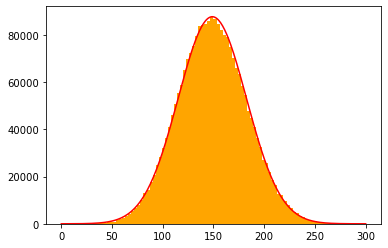
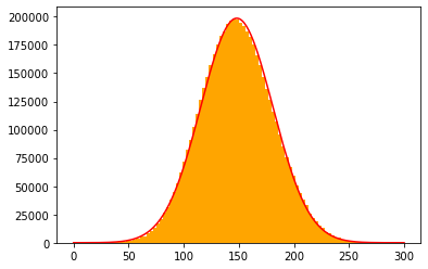
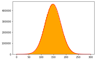
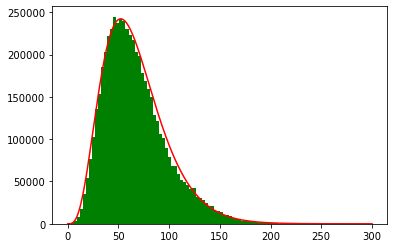
Figure 1 has the histograms of $r$-loadings of $\mathbf{t}\in\mathcal{P}(n)^{3}$ for $n=14,15,16$. According to what the histograms suggest, we conjecture that the distribution of the $r$-loadings of $\mathbf{t}$ converges to a normal distribution as $n\to\infty$, and sketch the curves of normal distributions on the histograms. Here we note that the mean is not exactly 150. Actually, the mean values of the $r$-loadings are $\approx 148.86,148.15,147.65$ for $n=14,15,16$, respectively.

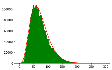
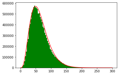
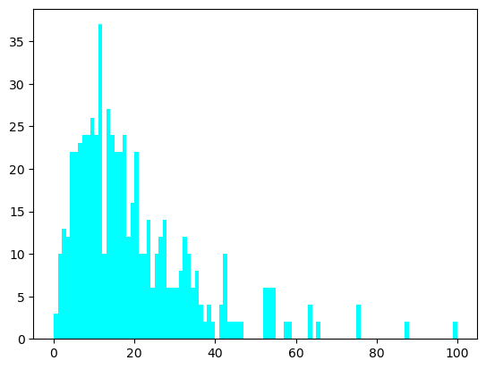
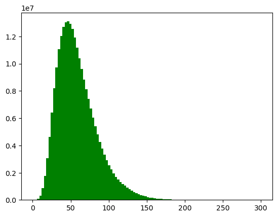
Similarly, Figure 2 shows the histograms of $b$-loadings of $\mathbf{t}\in\mathcal{P}(n)^{3}$ for $n=14,15,16$, and we conjecture that the distribution of the $b$-loadings of $\mathbf{t}$ is a gamma distribution as $n\to\infty$, and draw the curves of gamma distributions on the histograms. The mean values of the $b$-loadings are $\approx 72.07,66.71,63.48$ for $n=14,15,16$, respectively.

Figure 1. Histograms of $r$-loadings of $\mathbf{t}\in\mathcal{P}(n)^{3}$ for $n=14,15,16$ from left to right along with curves (red) of normal distributions

Figure 2. Histograms of $b$-loadings of $\mathbf{t}\in\mathcal{P}(n)^{3}$ for $n=14,15,16$ from left to right along with curves (red) of gamma distributions

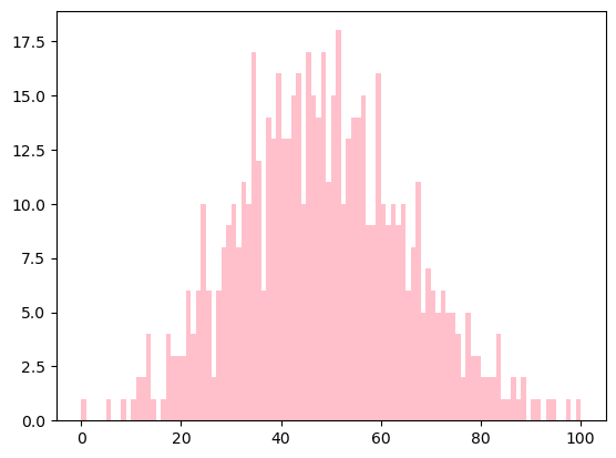
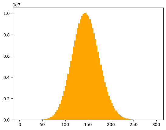
When $n=14,15,16$, the histograms of loadings of partitions $\lambda\in\mathcal{P}(n)$ do not have enough number of points to tell which distributions they follow. (Note that $p(16)=231$.) Nonetheless, it seems reasonable to expect that the $r$-loadings of $\lambda$ follow a normal distribution and that the $b$-loadings of $\lambda$ follow a gamma distribution. Then the loadings of $\mathbf{t}\in\mathcal{P}(n)^{3}$ will have the distributions given as a sum of three independent distributions. (Recall Definition 2.7.) Figure 3 has the histograms of loadings of $\lambda$ and $\mathbf{t}$ when $n=20$, which seem to be consistent with this expectation.

Figure 3. Histograms of $r$-loadings of $\lambda\in\mathcal{P}(n)$ (top-left) and $\mathbf{t}\in\mathcal{P}(n)^{3}$ (top-right) and histograms of $b$-loadings of $\lambda$ (bottom-left) and $\mathbf{t}$ (bottom-right) when $n=20$

4. Separation of $g(\mathbf{t})\neq 0$ from $g(\mathbf{t})=0$

In this section, we consider the distributions of loadings according to whether the Kronecker coefficients $g(\mathbf{t})$ are zero or nonzero. Using minimum values of loadings in each case, we will obtain vertical lines which separate the distributions of these two cases.

In Figures 4–7, we present the ranges and histograms of loadings of $\mathbf{t}\in\mathcal{P}(n)^{3}$ for $n=10,11,12,13$ according to whether $g(\mathbf{t})\neq 0$ (red) or $=0$ (blue). As one can see, the ranges and histograms do not vary much as $n$ varies. The separation between the regions corresponding to $g(\mathbf{t})\neq 0$ (red) and $=0$ (blue) is more distinctive in the case of $b$-loadings. It is clear that we may use the minimum values of loadings to obtain vertical lines that separate the red regions from the blue ones.

Figure 4. Ranges of $r$-loadings for $n=10,11,12,13$ from top to bottom. A red (resp. blue) dot at $(x,1)$ (resp. $(x,0)$) corresponds to $\mathbf{t}\in\mathcal{P}(n)^{3}$ with $r(\mathbf{t})=x$ and $g(\mathbf{t})\neq 0$ (resp. $g(\mathbf{t})=0$).

Figure 5. Histograms of $r$-loadings for $n=10$ (top-left), $11$ (top-right), $12$ (bottom-left) and $13$ (bottom-right). The red (resp. blue) region represents the numbers of $\mathbf{t}$ such that $g(\mathbf{t})\neq 0$ (resp. $g(\mathbf{t})=0$).

Figure 6. Ranges of $b$-loadings for $n=10,11,12,13$ from top to bottom. A red (resp. blue) dot at $(x,1)$ (resp. $(x,0)$) corresponds to $\mathbf{t}\in\mathcal{P}(n)^{3}$ with $b(\mathbf{t})=x$ and $g(\mathbf{t})\neq 0$ (resp. $g(\mathbf{t})=0$).

Figure 7. Histograms of $b$-loadings for $n=10$ (top-left), $11$ (top-right), $12$ (bottom-left) and $13$ (bottom-right). The red (resp. blue) region represents the numbers of $\mathbf{t}$ such that $g(\mathbf{t})\neq 0$ (resp. $g(\mathbf{t})=0$).

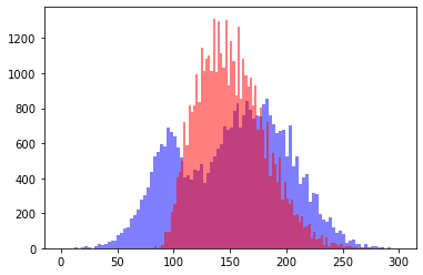
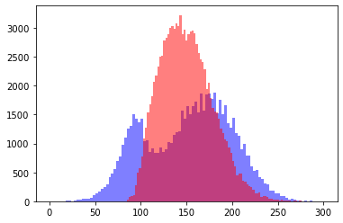
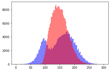
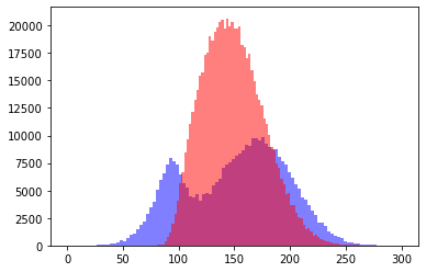
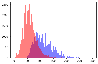
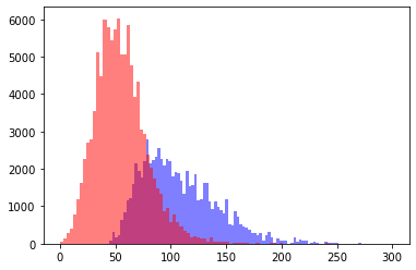
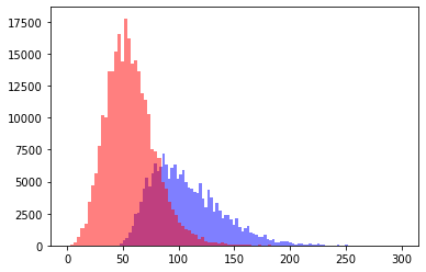
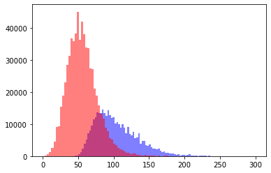
With this in mind, define

$$r_{\star} \coloneqq\min\{r(\mathbf{t}):g(\mathbf{t})\neq 0,\mathbf{t}\in\mathcal{P}(n)^{3}\}\quad\text{ and }$$

$$b_{\star} \coloneqq\min\{b(\mathbf{t}):g(\mathbf{t})=0,\mathbf{t}\in\mathcal{P}(n)^{3}\}.$$

Then, for $\mathbf{t}\in\mathcal{P}(n)^{3}$,

(4.1) $$\text{ if }r(\mathbf{t})<r_{\star}\text{ then }g(\mathbf{t})=0\ \text{ and }\ \boxed{\text{if }b(\mathbf{t})<b_{\star}\text{ then }g(\mathbf{t})\neq 0}.$$

This provides sufficient conditions for $g(\mathbf{t})=0$ and $g(\mathbf{t})\neq 0$, respectively, once we know the values of $r_{\star}$ and $b_{\star}$. However, the values $r_{\star}$ do not turn out to be very useful for bigger $n$ in distinguishing $g(\mathbf{t})=0$ from $g(\mathbf{t})\neq 0$, though they are interesting for their own sake and can be useful for further analysis. See Example 4.2 (2).

Remark 4.1.

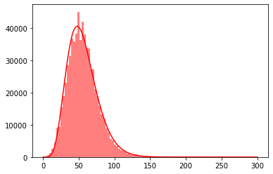
It appears that the $b$-loadings of $\mathbf{t}$ with $g(\mathbf{t})\neq 0$ is a gamma distribution by itself. See the histogram and the curve of a gamma distribution when $n=13$ in Figure 8.

Figure 8. Histogram and curve (red) of a gamma distribution when $n=13$

In the rest of this section, computational results of the values of $r_{\star}$ and $b_{\star}$ for $6\leq n\leq 20$ will be presented along with some conjectures. This information can be used very effectively as illustrated in the example below.

Example 4.2.

1. When $n=18$, we obtain $b_{\star}\approx 44.18$. Now that the $b$-loading of

   $$\mathbf{t}=((12,4,2),(8,4,2,2,1,1),(5,4,3,3,1,1,1))$$

   is readily computed to be approximately $41.07<b_{\star}$, we immediately conclude that $g(\mathbf{t})\neq 0$ by (4.1).

2. When $n=20$, there are $246,491,883$ triples $\mathbf{t}\in\mathcal{P}(20)$. Among them, $78,382,890$ triples satisfy $b(\mathbf{t})<b_{\star}\approx 43.74$ so that $g(\mathbf{t})\neq 0$. The percentage of these triples is about 31.8%. In contrast, $909,200$ triples satisfy $r(\mathbf{t})<r_{\star}\approx 70.88$ and the percentage is only $0.37\%$.

4.1. $r$-loadings results

We compute and record $r_{\star}$ and $\mathbf{t}=(\lambda,\mu,\nu)$ such that $r_{\star}=r(\mathbf{t})$ and $\lambda\geq\mu\geq\nu$ lexicographically, for $6\leq n\leq 20$ in Table 1. We do not consider $n\leq 5$ because they seem to be too small for statistical analysis.

$n$	$r_{\star}$	LL $\lambda$	LLL $\mu$	LLLL $\nu$
6	90.9986	$(3,3)$	$(2,2,2)$	$(1,1,1,1,1,1)$
7	85.0932	$(2,2,2,1)$	$(2,2,2,1)$	$(2,2,2,1)$
8	79.1637	$(2^{4})$	$(2^{4})$	$(2^{4})$
9	84.5605	$(3,2,2,2)$	$(2,2,2,2,1)$	$(2,2,2,2,1)$
10	82.5959	$(3,3,2,2)$	$(2,2,2,2,2)$	$(2,2,2,2,1,1)$
11	78.1018	$(3,3,3,2)$	$(2^{5},1)$	$(2^{5},1)$
12	74.6018	$(3^{4})$	$(2^{6})$	$(2^{6})$
13	78.1813	$(4,3,3,3)$	$(2^{6},1)$	$(2^{6},1)$
14	77.3651	$(4,4,3,3)$	$(2^{7})$	$(2^{6},1,1)$
15	74.8437	$(4,4,4,3)$	$(2^{7},1)$	$(2^{7},1)$
16	72.1837	$(4^{4})$	$(2^{8})$	$(2^{8})$
17	71.2716	$(3^{5},2)$	$(3^{5},2)$	$(2^{8},1)$
18	68.9559	$(3^{6})$	$(3^{6})$	$(2^{9})$
19	71.9678	$(4,3^{5})$	$(3^{6},1)$	$(2^{9},1)$
20	70.8806	$(5^{4})$	$(2^{10})$	$(2^{10})$

Table 1. Values of $r_{\star}$ and $\mathbf{t}=(\lambda,\mu,\nu)$ such that $r_{\star}=r(\mathbf{t})$ and $\lambda\geq\mu\geq\nu$ lexicographically

Based on the results of $n=8,12,16,20$ as written in blue in Table 1, we make the following conjecture.

Conjecture 4.3.

When $n=4k$ ($k\geq 2$), the values $r_{\star}$ are attained by $\mathbf{t}=((k^{4}),(2^{2k}),(2^{2k}))$.

As an exhaustive computation for all possible triples becomes exponentially expensive, we assume that Conjecture 4.3 is true and continue computation. The results are in Table 2. Since we know $\mathbf{t}$ exactly under Conjecture 4.3, we could calculate $r_{\star}$ for $n$ much bigger than those $n$ in the case of $b_{\star}$ that will be presented in Table 4.

$n$	$r_{\star}$	LLLLL $\mathbf{t}$
24	70.0772	$((6^{4}),(2^{12}),(2^{12}))$
28	69.5351	$((7^{4}),(2^{14}),(2^{14}))$
32	69.1732	$((8^{4}),(2^{16}),(2^{16}))$
36	68.9254	$((9^{4}),(2^{18}),(2^{18}))$
40	68.7518	$((10^{4}),(2^{20}),(2^{20}))$
44	68.6334	$((11^{4}),(2^{22}),(2^{22}))$
48	68.5549	$((12^{4}),(2^{24}),(2^{24}))$

Table 2. Under Conjecture 4.3, values of $r_{\star}$ and $\mathbf{t}=((k^{4}),(2^{2k}),(2^{2k}))$ for $n=4k$ such that $r_{\star}=r(\mathbf{t})$

Remark 4.4.

The values of $r_{\star}$ seem to keep decreasing though slowly. However, it is not clear whether $r_{\star}$ becomes bounded or not as $n\to\infty$.

Notice that we have a sufficient condition for $g(\mathbf{t})=0$ by taking the contrapositive of (2.1):

(4.2) $$d_{\nu}<|d_{\lambda}-d_{\mu}|\quad\text{ or }\quad d_{\nu}>d_{\lambda}+d_{\mu}\quad\Longrightarrow\quad g(\mathbf{t})=0.$$

As $r_{\star}$ provides another sufficient condition for $g(\mathbf{t})=0$ in (4.1), one may be curious about their relationship. As a matter of fact, we observe that

$$r_{\star}<r(\mathbf{t})\quad\text{ for any $\mathbf{t}$ satisfying the condition in \eqref{eqn-dl-1}}.$$

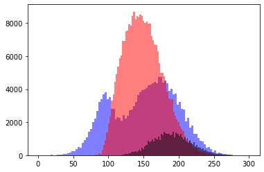
Thus conditions in (4.1) and (4.2) for $g(\mathbf{t})=0$ do not have overlaps. Let us look at pictures when $n=12$. In the graph of Figure 9, red dots and blue dots are as before, while a black dot at $(x,\frac{1}{2})$ corresponds to $\mathbf{t}\in\mathcal{P}(12)^{3}$ satisfying the condition in (4.2) with $r(\mathbf{t})=x$ and $g(\mathbf{t})=0$. In the histograms of Figure 9, the red region and blue region are as before, while the dark brown region represents the numbers of $\mathbf{t}$ satisfying the condition in (4.2) and $g(\mathbf{t})=0$.

Figure 9. Ranges of $r$-loadings where a black dot at $(x,\frac{1}{2})$ corresponds to $\mathbf{t}\in\mathcal{P}(12)^{3}$ satisfying the condition in (4.2) with $r(\mathbf{t})=x$ and $g(\mathbf{t})=0$ and histograms of $r$-loadings where the dark brown region represents the numbers of $\mathbf{t}$ satisfying the condition in (4.2) and $g(\mathbf{t})=0$.

4.2. $b$-loadings results

In Table 3, we record $b_{\star}$ and $\mathbf{t}=(\lambda,\mu,\nu)$ such that $b_{\star}=b(\mathbf{t})$ and $\lambda\geq\mu\geq\nu$ lexicographically, for $6\leq n\leq 20$. When there are more than one $\mathbf{t}$ such that $b_{\star}=b(\mathbf{t})$, we only record the lexicographically smallest one. (Recall (2.2).) For example, when $n=16$, we have $b_{\star}=b(\mathbf{t}_{1})=b(\mathbf{t}_{2})=b(\mathbf{t}_{3})$ with

$$\mathbf{t}_{1} =[(10,3,2,1),(10,3,2,1),(5,3,2,1^{6})],$$

$$\mathbf{t}_{2} =[(10,3,2,1),(9,3,2,1,1),(4,3,2,1^{7})],$$

$$\mathbf{t}_{3} =[(5,3,2,1^{6}),(4,3,2,1^{7}),(4,3,2,1^{7})],$$

and only $\mathbf{t}_{3}$ is recorded in the table.

$n$	$b_{\star}$	LLLL $\lambda$	LLLL $\mu$	LLLL $\nu$
6	59.7812	$(2,2,1,1)$	$(2,2,1,1)$	$(2,2,1,1)$
7	47.9477	$(3,3,1)$	$(3,1,1,1,1)$	$(3,1,1,1,1)$
8	54.6650	$(3,2,1,1,1)$	$(3,2,1,1,1)$	$(2,2,1,1,1,1)$
9	39.8213	$(3,2,1,1,1,1)$	$(3,2,1,1,1,1)$	$(3,2,1,1,1,1)$
10	46.6592	$(4,2,1^{4})$	$(3,2,1^{5})$	$(3,2,1^{5})$
11	44.4953	$(6,1^{5})$	$(6,1^{5})$	$(4,3,3,1)$
12	47.3571	$(3,3,2,1^{4})$	$(3,3,2,1^{4})$	$(3,3,2,1^{4})$
13	45.1104	$(4,3,2,1^{4})$	$(3,3,2,1^{5})$	$(3,3,2,1^{5})$
14	44.9312	$(4,3,2,1^{5})$	$(4,3,2,1^{5})$	$(3,3,2,1^{6})$
15	40.3916	$(4,3,2,1^{6})$	$(4,3,2,1^{6})$	$(4,3,2,1^{6})$
16	41.7064	$(5,3,2,1^{6})$	$(4,3,2,1^{7})$	$(4,3,2,1^{7})$
17	43.4181	$(5,3,2,1^{7})$	$(4,3,2,2,1^{6})$	$(4,3,2,2,1^{6})$
18	44.1817	$(4,4,2,2,1^{6})$	$(4,4,2,2,1^{6})$	$(4,4,2,2,1^{6})$
19	44.3797	$(5,4,2,2,1^{6})$	$(4,4,2,2,1^{7})$	$(4,4,2,2,1^{7})$
20	43.7424	$(5,4,2,2,1^{7})$	$(4,4,3,2,1^{7})$	$(4,4,3,2,1^{7})$

Table 3. Values of $b_{\star}$ and $\mathbf{t}=(\lambda,\mu,\nu)$ such that $b_{\star}=b(\mathbf{t})$

Based on the results in Table 3—in particular, on the results of $n=6,9,12,15,18$ as written in blue—we make the following conjecture.

Conjecture 4.5.

For $n\geq 6$, the values $b_{\star}$ are attained by $\mathbf{t}=(\lambda,\mu,\nu)$ such that $\lambda=\mu$ or $\mu=\nu$. Moreover, when $n=3k$, $k\geq 2$, the values $b_{\star}$ are attained by $\mathbf{t}=(\lambda,\mu,\nu)$ such that $\lambda=\mu=\nu$.

As an exhaustive computation for all possible triples becomes exponentially expensive, we assume that Conjecture 4.5 is true for $n=3k$ and continue computation. The results are in Table 4.

$n$	$b_{\star}$	LL $\lambda=\mu=\nu$
21	45.0545	$(5,4,2,2,1^{8})$
24	43.7126	$(5,4,3,2,2,1^{8})$
27	44.0699	$(5,5,3,3,2,1^{9})$
30	45.0141	$(5,5,4,3,2,2,1^{9})$
33	44.7615	$(6,6,4,3,2,1^{12})$
36	44.3350	$(6,6,4,3,2^{3},1^{11})$

Table 4. Under Conjecture 4.5, values of $b_{\star}$ and $\mathbf{t}=(\lambda,\lambda,\lambda)$ for $n=3k$ such that $b_{\star}=b(\mathbf{t})$

Remark 4.6.

The values of $b_{\star}$ seem to be fluctuating with decreasing amplitudes as $n$ increases. However, it is not clear if $b_{\star}$ converges as $n\to\infty$.

Appendix A Table of Loadings

We tabulate the $r$-loading $r_{\lambda}$ and $b$-loading $b_{\lambda}$ of each partition $\lambda\in\mathcal{P}(n)$ for $6\leq n\leq 12$.

$\lambda$	$r_{\lambda}$	$b_{\lambda}$
$(6,0,0,0,0,0)$	100.0	100.0
$(5,1,0,0,0,0)$	85.8934	37.252
$(4,2,0,0,0,0)$	71.7868	19.9271
$(4,1,1,0,0,0)$	66.6591	4.363
$(3,3,0,0,0,0)$	57.6803	43.005
$(3,2,1,0,0,0)$	52.5526	0.0
$(3,1,1,1,0,0)$	45.2311	4.363
$(2,2,2,0,0,0)$	33.3183	43.005
$(2,2,1,1,0,0)$	31.1245	19.9271
$(2,1,1,1,1,0)$	22.8133	37.252
$(1,1,1,1,1,1)$	0.0	100.0
$(7,0,0,0,0,0,0)$	100.0	100.0
$(6,1,0,0,0,0,0)$	88.302	47.507
$(5,2,0,0,0,0,0)$	76.604	26.483
$(5,1,1,0,0,0,0)$	72.8338	13.1061
$(4,3,0,0,0,0,0)$	64.906	36.928
$(4,2,1,0,0,0,0)$	61.1358	0.0
$(4,1,1,1,0,0,0)$	55.5306	1.81
$(3,3,1,0,0,0,0)$	49.4378	21.735
$(3,2,2,0,0,0,0)$	45.6676	21.735
$(3,2,1,1,0,0,0)$	43.8326	0.0
$(3,1,1,1,1,0,0)$	37.3978	13.1061
$(2,2,2,1,0,0,0)$	28.3644	36.928
$(2,2,1,1,1,0,0)$	25.6998	26.483
$(2,1,1,1,1,1,0)$	18.7933	47.507
$(1,1,1,1,1,1,1)$	0.0	100.0
$(8,0,0,0,0,0,0,0)$	100.0	100.0
$(7,1,0,0,0,0,0,0)$	90.5921	58.055
$(6,2,0,0,0,0,0,0)$	81.1842	35.198
$(6,1,1,0,0,0,0,0)$	77.6539	28.246
$(5,3,0,0,0,0,0,0)$	71.7763	34.854
$(5,2,1,0,0,0,0,0)$	68.2461	9.7331
$(5,1,1,1,0,0,0,0)$	63.194	12.637
$(4,4,0,0,0,0,0,0)$	62.3685	48.552
$(4,3,1,0,0,0,0,0)$	58.8382	15.265
$(4,2,2,0,0,0,0,0)$	55.3079	15.265
$(4,2,1,1,0,0,0,0)$	53.7861	0.0
$(4,1,1,1,1,0,0,0)$	47.8449	12.637
$(3,3,2,0,0,0,0,0)$	45.9	30.531
$(3,3,1,1,0,0,0,0)$	44.3782	15.265
$(3,2,2,1,0,0,0,0)$	40.8479	15.265
$(3,2,1,1,1,0,0,0)$	38.437	9.7331
$(3,1,1,1,1,1,0,0)$	32.0837	28.246
$(2,2,2,2,0,0,0,0)$	26.3879	48.552
$(2,2,2,1,1,0,0,0)$	25.4988	34.854
$(2,2,1,1,1,1,0,0)$	22.6758	35.198
$(2,1,1,1,1,1,1,0)$	16.0886	58.055
$(1,1,1,1,1,1,1,1)$	0.0	100.0
$(9,0,0,0,0,0,0,0,0)$	100.0	100.0
$(8,1,0,0,0,0,0,0,0)$	91.876	62.802
$(7,2,0,0,0,0,0,0,0)$	83.7521	39.559
$(7,1,1,0,0,0,0,0,0)$	80.9205	33.587
$(6,3,0,0,0,0,0,0,0)$	75.6281	34.591
$(6,2,1,0,0,0,0,0,0)$	72.7965	13.273
$(6,1,1,1,0,0,0,0,0)$	68.4825	16.425
$(5,4,0,0,0,0,0,0,0)$	67.5041	42.455
$(5,3,1,0,0,0,0,0,0)$	64.6726	12.1941
$(5,2,2,0,0,0,0,0,0)$	61.841	12.1941

$\lambda$	$r_{\lambda}$	$b_{\lambda}$
$(5,2,1,1,0,0,0,0,0)$	60.3586	0.0
$(5,1,1,1,1,0,0,0,0)$	55.3152	10.278
$(4,4,1,0,0,0,0,0,0)$	56.5486	26.205
$(4,3,2,0,0,0,0,0,0)$	53.7171	17.261
$(4,3,1,1,0,0,0,0,0)$	52.2346	5.067
$(4,2,2,1,0,0,0,0,0)$	49.4031	5.067
$(4,2,1,1,1,0,0,0,0)$	47.1912	0.0
$(4,1,1,1,1,1,0,0,0)$	41.7289	16.425
$(3,3,3,0,0,0,0,0,0)$	42.7616	39.778
$(3,3,2,1,0,0,0,0,0)$	41.2791	17.261
$(3,3,1,1,1,0,0,0,0)$	39.0672	12.1941
$(3,2,2,2,0,0,0,0,0)$	36.9651	26.205
$(3,2,2,1,1,0,0,0,0)$	36.2357	12.1941
$(3,2,1,1,1,1,0,0,0)$	33.6049	13.273
$(3,1,1,1,1,1,1,0,0)$	27.9202	33.587
$(2,2,2,2,1,0,0,0,0)$	23.7977	42.455
$(2,2,2,1,1,1,0,0,0)$	22.6494	34.591
$(2,2,1,1,1,1,1,0,0)$	19.7962	39.559
$(2,1,1,1,1,1,1,1,0)$	13.9854	62.802
$(1,1,1,1,1,1,1,1,1)$	0.0	100.0
$(10,0,0,0,0,0,0,0,0,0)$	100.0	100.0
$(9,1,0,0,0,0,0,0,0,0)$	93.0766	67.7441
$(8,2,0,0,0,0,0,0,0,0)$	86.1532	45.12
$(8,1,1,0,0,0,0,0,0,0)$	83.5036	41.476
$(7,3,0,0,0,0,0,0,0,0)$	79.2298	36.947
$(7,2,1,0,0,0,0,0,0,0)$	76.5802	20.739
$(7,1,1,1,0,0,0,0,0,0)$	72.6788	23.437
$(6,4,0,0,0,0,0,0,0,0)$	72.3065	39.542
$(6,3,1,0,0,0,0,0,0,0)$	69.6568	15.044
$(6,2,2,0,0,0,0,0,0,0)$	67.0072	15.044
$(6,2,1,1,0,0,0,0,0,0)$	65.7554	5.179
$(6,1,1,1,1,0,0,0,0,0)$	61.1395	14.455
$(5,5,0,0,0,0,0,0,0,0)$	65.3831	49.1901
$(5,4,1,0,0,0,0,0,0,0)$	62.7334	21.441
$(5,3,2,0,0,0,0,0,0,0)$	60.0838	13.151
$(5,3,1,1,0,0,0,0,0,0)$	58.832	3.286
$(5,2,2,1,0,0,0,0,0,0)$	56.1824	3.286
$(5,2,1,1,1,0,0,0,0,0)$	54.2161	0.0
$(5,1,1,1,1,1,0,0,0,0)$	49.2041	14.455
$(4,4,2,0,0,0,0,0,0,0)$	53.1604	24.72
$(4,4,1,1,0,0,0,0,0,0)$	51.9086	14.862
$(4,3,3,0,0,0,0,0,0,0)$	50.5108	27.307
$(4,3,2,1,0,0,0,0,0,0)$	49.259	6.572
$(4,3,1,1,1,0,0,0,0,0)$	47.2927	3.286
$(4,2,2,2,0,0,0,0,0,0)$	45.3575	14.862
$(4,2,2,1,1,0,0,0,0,0)$	44.6431	3.286
$(4,2,1,1,1,1,0,0,0,0)$	42.2807	5.179
$(4,1,1,1,1,1,1,0,0,0)$	37.0369	23.437
$(3,3,3,1,0,0,0,0,0,0)$	39.686	27.307
$(3,3,2,2,0,0,0,0,0,0)$	38.4341	24.72
$(3,3,2,1,1,0,0,0,0,0)$	37.7197	13.151
$(3,3,1,1,1,1,0,0,0,0)$	35.3573	15.044
$(3,2,2,2,1,0,0,0,0,0)$	33.8182	21.441
$(3,2,2,1,1,1,0,0,0,0)$	32.7077	15.044
$(3,2,1,1,1,1,1,0,0,0)$	30.1135	20.739
$(3,1,1,1,1,1,1,1,0,0)$	24.747	41.476
$(2,2,2,2,2,0,0,0,0,0)$	22.2789	49.1901
$(2,2,2,2,1,1,0,0,0,0)$	21.8828	39.542

$\lambda$	$r_{\lambda}$	$b_{\lambda}$
$(2,2,2,1,1,1,1,0,0,0)$	20.5405	36.947
$(2,2,1,1,1,1,1,1,0,0)$	17.8237	45.12
$(2,1,1,1,1,1,1,1,1,0)$	12.3875	67.7441
$(1,1,1,1,1,1,1,1,1,1)$	0.0	100.0
$(11,0,0,0,0,0,0,0,0,0,0)$	100.0	100.0
$(10,1,0,0,0,0,0,0,0,0,0)$	93.8295	71.265
$(9,2,0,0,0,0,0,0,0,0,0)$	87.6591	49.697
$(9,1,1,0,0,0,0,0,0,0,0)$	85.397	46.624
$(8,3,0,0,0,0,0,0,0,0,0)$	81.4886	39.924
$(8,2,1,0,0,0,0,0,0,0,0)$	79.2265	26.3731
$(8,1,1,1,0,0,0,0,0,0,0)$	75.8034	28.711
$(7,4,0,0,0,0,0,0,0,0,0)$	75.3182	39.780
$(7,3,1,0,0,0,0,0,0,0,0)$	73.0561	18.329
$(7,2,2,0,0,0,0,0,0,0,0)$	70.794	18.329
$(7,2,1,1,0,0,0,0,0,0,0)$	69.6329	10.1901
$(7,1,1,1,1,0,0,0,0,0,0)$	65.58	17.872
$(6,5,0,0,0,0,0,0,0,0,0)$	69.1477	45.913
$(6,4,1,0,0,0,0,0,0,0,0)$	66.8856	20.801
$(6,3,2,0,0,0,0,0,0,0,0)$	64.6236	12.90
$(6,3,1,1,0,0,0,0,0,0,0)$	63.4625	4.762
$(6,2,2,1,0,0,0,0,0,0,0)$	61.2004	4.762
$(6,2,1,1,1,0,0,0,0,0,0)$	59.4095	1.967
$(6,1,1,1,1,1,0,0,0,0,0)$	54.969	14.412
$(5,5,1,0,0,0,0,0,0,0,0)$	60.7152	30.394
$(5,4,2,0,0,0,0,0,0,0,0)$	58.4531	18.834
$(5,4,1,1,0,0,0,0,0,0,0)$	57.292	10.694
$(5,3,3,0,0,0,0,0,0,0,0)$	56.191	21.014
$(5,3,2,1,0,0,0,0,0,0,0)$	55.0299	2.795
$(5,3,1,1,1,0,0,0,0,0,0)$	53.2391	0.0
$(5,2,2,2,0,0,0,0,0,0,0)$	51.6068	10.694
$(5,2,2,1,1,0,0,0,0,0,0)$	50.977	0.0
$(5,2,1,1,1,1,0,0,0,0,0)$	48.7986	1.967
$(5,1,1,1,1,1,1,0,0,0,0)$	44.1465	17.872
$(4,4,3,0,0,0,0,0,0,0,0)$	50.0206	31.70
$(4,4,2,1,0,0,0,0,0,0,0)$	48.8595	13.4
$(4,4,1,1,1,0,0,0,0,0,0)$	47.0686	10.694
$(4,3,3,1,0,0,0,0,0,0,0)$	46.5974	15.6
$(4,3,2,2,0,0,0,0,0,0,0)$	45.4363	13.4
$(4,3,2,1,1,0,0,0,0,0,0)$	44.8065	2.795
$(4,3,1,1,1,1,0,0,0,0,0)$	42.6281	4.762
$(4,2,2,2,1,0,0,0,0,0,0)$	41.3834	10.694
$(4,2,2,1,1,1,0,0,0,0,0)$	40.366	4.762
$(4,2,1,1,1,1,1,0,0,0,0)$	37.9761	10.1901
$(4,1,1,1,1,1,1,1,0,0,0)$	33.1883	28.711
$(3,3,3,2,0,0,0,0,0,0,0)$	37.0038	31.70
$(3,3,3,1,1,0,0,0,0,0,0)$	36.374	21.014
$(3,3,2,2,1,0,0,0,0,0,0)$	35.2129	18.834
$(3,3,2,1,1,1,0,0,0,0,0)$	34.1956	12.90
$(3,3,1,1,1,1,1,0,0,0,0)$	31.8056	18.329
$(3,2,2,2,2,0,0,0,0,0,0)$	31.1599	30.394
$(3,2,2,2,1,1,0,0,0,0,0)$	30.7724	20.801
$(3,2,2,1,1,1,1,0,0,0,0)$	29.5435	18.329
$(3,2,1,1,1,1,1,1,0,0,0)$	27.0179	26.3731
$(3,1,1,1,1,1,1,1,1,0,0)$	22.1582	46.624
$(2,2,2,2,2,1,0,0,0,0,0)$	20.549	45.913
$(2,2,2,2,1,1,1,0,0,0,0)$	19.9499	39.780
$(2,2,2,1,1,1,1,1,0,0,0)$	18.5853	39.924
$(2,2,1,1,1,1,1,1,1,0,0)$	15.9878	49.697
$(2,1,1,1,1,1,1,1,1,1,0)$	11.0873	71.265
$(1,1,1,1,1,1,1,1,1,1,1)$	0.0	100.0
$(12,0,0,0,0,0,0,0,0,0,0,0)$	100.0	100.0
$(11,1,0,0,0,0,0,0,0,0,0,0)$	94.5958	74.832
$(10,2,0,0,0,0,0,0,0,0,0,0)$	89.1916	54.707

$\lambda$	$r_{\lambda}$	$b_{\lambda}$
$(10,1,1,0,0,0,0,0,0,0,0,0)$	87.0838	52.743
$(9,3,0,0,0,0,0,0,0,0,0,0)$	83.7874	43.844
$(9,2,1,0,0,0,0,0,0,0,0,0)$	81.6796	33.490
$(9,1,1,1,0,0,0,0,0,0,0,0)$	78.5079	35.703
$(8,4,0,0,0,0,0,0,0,0,0,0)$	78.3831	41.257
$(8,3,1,0,0,0,0,0,0,0,0,0)$	76.2754	23.775
$(8,2,2,0,0,0,0,0,0,0,0,0)$	74.1676	23.775
$(8,2,1,1,0,0,0,0,0,0,0,0)$	73.1037	17.598
$(8,1,1,1,1,0,0,0,0,0,0,0)$	69.3148	24.48
$(7,5,0,0,0,0,0,0,0,0,0,0)$	72.9789	44.246
$(7,4,1,0,0,0,0,0,0,0,0,0)$	70.8711	22.913
$(7,3,2,0,0,0,0,0,0,0,0,0)$	68.7634	15.785
$(7,3,1,1,0,0,0,0,0,0,0,0)$	67.6995	9.608
$(7,2,2,1,0,0,0,0,0,0,0,0)$	65.5917	9.608
$(7,2,1,1,1,0,0,0,0,0,0,0)$	63.9106	8.104
$(7,1,1,1,1,1,0,0,0,0,0,0)$	59.7695	18.845
$(6,6,0,0,0,0,0,0,0,0,0,0)$	67.5747	50.894
$(6,5,1,0,0,0,0,0,0,0,0,0)$	65.4669	28.138
$(6,4,2,0,0,0,0,0,0,0,0,0)$	63.3591	17.15
$(6,4,1,1,0,0,0,0,0,0,0,0)$	62.2953	10.981
$(6,3,3,0,0,0,0,0,0,0,0,0)$	61.2514	19.530
$(6,3,2,1,0,0,0,0,0,0,0,0)$	60.1875	3.854
$(6,3,1,1,1,0,0,0,0,0,0,0)$	58.5064	2.350
$(6,2,2,2,0,0,0,0,0,0,0,0)$	57.0159	10.981
$(6,2,2,1,1,0,0,0,0,0,0,0)$	56.3986	2.350
$(6,2,1,1,1,1,0,0,0,0,0,0)$	54.3653	4.700
$(6,1,1,1,1,1,1,0,0,0,0,0)$	49.9969	18.845
$(5,5,2,0,0,0,0,0,0,0,0,0)$	57.9549	25.7881
$(5,5,1,1,0,0,0,0,0,0,0,0)$	56.8911	19.6111
$(5,4,3,0,0,0,0,0,0,0,0,0)$	55.8471	24.3081
$(5,4,2,1,0,0,0,0,0,0,0,0)$	54.7833	8.631
$(5,4,1,1,1,0,0,0,0,0,0,0)$	53.1022	7.127
$(5,3,3,1,0,0,0,0,0,0,0,0)$	52.6755	11.003
$(5,3,2,2,0,0,0,0,0,0,0,0)$	51.6117	8.631
$(5,3,2,1,1,0,0,0,0,0,0,0)$	50.9944	0.0
$(5,3,1,1,1,1,0,0,0,0,0,0)$	48.9611	2.350
$(5,2,2,2,1,0,0,0,0,0,0,0)$	47.8227	7.127
$(5,2,2,1,1,1,0,0,0,0,0,0)$	46.8533	2.350
$(5,2,1,1,1,1,1,0,0,0,0,0)$	44.5927	8.104
$(5,1,1,1,1,1,1,1,0,0,0,0)$	40.099	24.48
$(4,4,4,0,0,0,0,0,0,0,0,0)$	48.3351	38.25
$(4,4,3,1,0,0,0,0,0,0,0,0)$	47.2713	19.634
$(4,4,2,2,0,0,0,0,0,0,0,0)$	46.2074	17.2631
$(4,4,2,1,1,0,0,0,0,0,0,0)$	45.5902	8.631
$(4,4,1,1,1,1,0,0,0,0,0,0)$	43.5569	10.981
$(4,3,3,2,0,0,0,0,0,0,0,0)$	44.0997	19.634
$(4,3,3,1,1,0,0,0,0,0,0,0)$	43.4824	11.003
$(4,3,2,2,1,0,0,0,0,0,0,0)$	42.4185	8.631
$(4,3,2,1,1,1,0,0,0,0,0,0)$	41.4491	3.854
$(4,3,1,1,1,1,1,0,0,0,0,0)$	39.1885	9.608
$(4,2,2,2,2,0,0,0,0,0,0,0)$	38.6296	19.6111
$(4,2,2,2,1,1,0,0,0,0,0,0)$	38.2774	10.981
$(4,2,2,1,1,1,1,0,0,0,0,0)$	37.0807	9.608
$(4,2,1,1,1,1,1,1,0,0,0,0)$	34.6948	17.598
$(4,1,1,1,1,1,1,1,1,0,0,0)$	30.1207	35.703
$(3,3,3,3,0,0,0,0,0,0,0,0)$	35.5238	38.25
$(3,3,3,2,1,0,0,0,0,0,0,0)$	34.9065	24.3081
$(3,3,3,1,1,1,0,0,0,0,0,0)$	33.9371	19.530
$(3,3,2,2,2,0,0,0,0,0,0,0)$	33.2254	25.7881
$(3,3,2,2,1,1,0,0,0,0,0,0)$	32.8732	17.15
$(3,3,2,1,1,1,1,0,0,0,0,0)$	31.6765	15.785
$(3,3,1,1,1,1,1,1,0,0,0,0)$	29.2906	23.775
$(3,2,2,2,2,1,0,0,0,0,0,0)$	29.0843	28.138

$\lambda$	$r_{\lambda}$	$b_{\lambda}$
$(3,2,2,2,1,1,1,0,0,0,0,0)$	28.5049	22.913
$(3,2,2,1,1,1,1,1,0,0,0,0)$	27.1828	23.775
$(3,2,1,1,1,1,1,1,1,0,0,0)$	24.7165	33.490
$(3,1,1,1,1,1,1,1,1,1,0,0)$	20.0998	52.743
$(2,2,2,2,2,2,0,0,0,0,0,0)$	19.539	50.894
$(2,2,2,2,2,1,1,0,0,0,0,0)$	19.3117	44.246
$(2,2,2,2,1,1,1,1,0,0,0,0)$	18.6069	41.257
$(2,2,2,1,1,1,1,1,1,0,0,0)$	17.2045	43.844
$(2,2,1,1,1,1,1,1,1,1,0,0)$	14.6956	54.707
$(2,1,1,1,1,1,1,1,1,1,1,0)$	10.0548	74.832
$(1,1,1,1,1,1,1,1,1,1,1,1)$	0.0	100.0

References

- [AHO] A. Ashmore, Y.-H. He, and B. A. Ovrut, Machine learning Calabi–Yau metrics, arXiv:1910.08605.
- [B] K. Buzzard, What is the point of computers? A question for pure mathematicians, arXiv:2112.11598.
- [CHKN] J. Carifio, J. Halverson, D. Krioukov, and B. D. Nelson, Machine learning in the string landscape, JHEP 157 (2017), no. 9.
- [DVB+] A. Davies, P. Veličković, L. Buesing, S. Blackwell, D. Zheng, N. Tomašev, R. Tanburn, P. Battaglia, C. Blundell, A. Juhász, M. Lackenby, G. Williamson, D. Hassabis and P. Kohli, Advancing mathematics by guiding human intuition with AI, Nature 600 (2021), 70–74.
- [DLQ] M. Douglas, S. Lakshminarasimhan and Y. Qi, Numerical Calabi–Yau metrics from holomorphic networks, Proceedings of Machine Learning Research 145 (2022), 223–252.
- [FH] W. Fulton and J. Harris, Representation theory, Graduate Texts in Mathematics, 129, Springer-Verlag, New York, 1991.
- [HTF] T. Hastie, R. Tibshirani, and J. Friedman, The elements of statistical learning: data mining, inference, and prediction, NY Springer, 2001.
- [HK] Y.-H. He and M. Kim, Learning algebraic structures: preliminary investigations, arXiv:1905.02263.
- [HLOa] Y.-H. He, K.-H. Lee, and T. Oliver, Machine-learning the Sato–Tate conjecture, J. Symb. Comput. 111 (2022), 61–72.
- [HLOb] by same author, Machine-learning number fields, Mathematics, Computation and Geometry of Data 2 (2022), 49–66.
- [HLOP] Y.-H. He, K.-H. Lee, T. Oliver, and A. Pozdnyakov, Murmurations of elliptic curves, arXiv:2204.10140.
- [JK] G. James and A. Kerber, em The representation theory of the symmetric group, Encyclopedia of Mathematics and its Applications 16, Addison-Wesley Publishing Co., Reading, Mass., 1981.
- [JKP] V. Jejjala, A. Kar, and O. Parrikar, Deep learning the hyperbolic volume of a knot, Phys. Lett. B, 799 (2019), 135033.
- [L] K.-H. Lee, Machine-learning Kronecker coefficients, arXiv:2306.04734.
- [W] G. Williamson, Is deep learning a useful tool for the pure mathematician?, arXiv:2304.12602.
- [Res] N. Ressayre, Horn inequalities for nonzero Kronecker coefficients, Adv. Math. 356 (2019) 106809.