Event Generation and Consistence Test for Physics with Sliced Wasserstein Distance

Abstract

In the field of modern high-energy physics research, there is a growing emphasis on utilizing deep learning techniques to optimize event simulation, thereby expanding the statistical sample size for more accurate physical analysis. Traditional simulation methods often encounter challenges when dealing with complex physical processes and high-dimensional data distributions, resulting in slow performance. To overcome these limitations, we propose a solution based on deep learning with the sliced Wasserstein distance as the loss function. Our method shows its ability on high precision and large-scale simulations, and demonstrates its effectiveness in handling complex physical processes. By employing an advanced transformer learning architecture, we initiate the learning process from a Monte Carlo sample, and generate high-dimensional data while preserving all original distribution features. The generated data samples have passed the consistence test, that is developed to calculate the confidence of the high-dimentional distributions of the generated data samples through permutation tests. This fast simulation strategy, enabled by deep learning, holds significant potential not only for increasing sample sizes and reducing statistical uncertainties but also for applications in numerical integration, which is crucial in partial wave analysis, high-precision sample checks, and other related fields. It opens up new possibilities for improving event simulation in high-energy physics research.

1 Introduction

In modern high-energy physics research, experimental data are increasingly complex and high-dimensional. For instance, a single particle collision event can generate numerous primary particles, each characterized by parameters such as momentum, energy, charge, and mass [1, 2]. Monte Carlo simulation is commonly employed to simulate particle collisions [3, 4, 5, 6, 7], but as the complexity of high-energy particle physics detectors grows, so does the intricacy of the detector simulation programs, resulting in higher costs [8, 9]. An example is from the LHCb experiment, where the limited statistics of $b\bar{b}\to D^{*-}3\pi^{\pm}X$ poses the largest systematic error in verifying lepton universality using $B^{0}\to D^{*-}\tau^{+}\nu_{\tau}$ [10]. This issue will be further exacerbated in future high-energy physics experiments like HL-LHC/CEPC/super-tau-charm [11, 12]. Consequently, the demand for simulation data will continue to rise as high-energy physics exploration deepens. Additionally, complex data necessitate sophisticated analysis tools, with partial wave analysis (PWA) being a powerful tool for handling angular distributions and extracting valuable information from intermediate resonances. However, PWA requires substantial simulation data, often requiring massive storage to obtain a sufficient number of independent simulation data samples [13]. This places significant demands on computing power and storage systems. Thus, finding methods to rapidly generate high-precision simulation data to reduce computing and storage requirements has become a crucial research objective.

Machine learning has demonstrated immense potential in event generation, with event generators frequently being trained on Generative Adversarial Networks (GANs) and Variational Autoencoders (VAEs) [14, 15, 16]. The objective is to learn the features of finite statistical data and rapidly generate large amounts of simulated data with consistent features. However, several challenging problems need to be addressed. In GANs, the generator aims to simulate the target data, while the discriminator tries to distinguish between the generated data and the target data [17]. Consequently, the training process can be unstable, and issues like model collapse may arise [18]. On the other hand, VAEs map input data to a probability distribution in latent space through an encoder and then reconstruct the original data space using latent variables and a decoder. VAEs may overlook crucial details in the data, necessitating a balance between the reconstruction error and the prior distribution error of the latent space [19]. When generating Monte Carlo distributions, the loss functions of VAEs and GANs are constructed based on individual events, leading to a natural problem. Their primary focus is to optimize physical laws or latent space distribution, rather than directly learning the distribution features of the original physical space. As a result, the generated data may not align well with the target data in terms of probability distribution.

To resolve this challenge, we propose the utilization of a novel loss function that captures the overall consistency between the target data and the generated data. However, the absence of a standardized measure, such as the one-dimensional KS test that directly quantifies the distance between high-dimensional samples, desires alternative approaches. Researchers often resort to constructing one-dimensional histogram distributions of relevant physical quantities or creating high-dimensional histograms to compare differences in each interval [20]. Nevertheless, this approach often leads to significant sparsity in higher dimensions, complicating data interpretation and analysis. Additionally, it is susceptible to outliers, which can distort the data distribution and hinder our understanding and analysis of the data [21]. Furthermore, this distance metric fails to provide an intuitive measure of the level of consistency between two samples’ distributions.

The Sliced Wasserstein Distance (SWD) presents a potential solution as an effective loss function. SWD quantifies the disparity between two probability distributions by slicing the probability distribution in multiple random directions, calculating the one-dimensional Wasserstein Distance in each direction, and averaging the distances across all directions to obtain the final SWD. In high-dimensional spaces, directly calculating the Wasserstein Distance becomes computationally complex [22]. However, SWD simplifies the high-dimensional problem into a computationally manageable one-dimensional problem, significantly reducing computational complexity and making it an ideal choice for handling high-dimensional data [23], comparing with other candidate loss function like Energy distance [24], Earth Mover’s Distance [25] and Chamfer distance [26]. With its continuous differentiability and high computational efficiency, SWD offers a promising approach to address the loss function problem and optimize model parameters to ensure that the generated data distribution closely approximates the real data distribution.

By combining the Sliced Wasserstein Distance with a permutation test [27, 28], we have successfully obtained a confidence indicator that quantitatively describes and compares distribution differences between high-dimensional data, as well as tests whether two data batches originate from the same distribution [29]. This confidence indicator is crucial in validating the accuracy of our generated data. The combined approach of Sliced Wasserstein Distance and permutation test is a powerful and flexible tool for studying high-dimensional data distributions, enabling comparison of data distributions from different models and assessment of disparities between experimental observations and theoretical predictions. It can provide vital support for practical activities like experimental simulation, data analysis, and serve as a reliable statistical testing method for high-dimensional data.

In this study, we used the $\psi(2S)$ decay data obtained from the BES III experiment, where the decay process is $\psi(2S)$ decaying into $\phi$ and $\pi^{+}$, $\pi^{-}$, and then $\phi$ further decaying into $K^{+}$, $K^{-}$. We used the Monte Carlo simulated data in the center-of-mass system and explored a novel way of using generative models, i.e., representing each unit of a single distribution as a token, and using the self-attention mechanism of Transformer to learn the relationships between these tokens  [30], thereby gaining a deep understanding of the target multivariate distribution. During the model optimization process, we used the Sliced Wasserstein Distance (SWD) and the Wasserstein distance for physical quantity as loss functions, and adjusted their weights with a gamma value. We measure the distribution gap between the model output and the target data directly instead of only optimizing the latent space like SWAE [31, 32], and finally construct a tool to calculate the confidence index to measure the degree of same distribution of high-dimensional data.

The structure of our paper will be divided into three main sections: results, discussion, and methods. In the results section, we will first compare our generated data with Monte Carlo simulated data by using some specific important one-dimensional physical quantities, such as the four-momentum, angles of the final state particles. This will be visually compared through histograms. Subsequently, we will use the Sliced Wasserstein Distance (SWD) and permutation test to calculate the confidence level, showcasing the differences in our generated data results under different model parameter settings, and demonstrating what kind of evaluation standards can accurately assess the data. In the discussion section, we will explore how we can make additional corrections based on specific physical analysis and specific detector information during the generation of instances. For instance, we may need to consider the efficiency of the detector and the dynamic factors of the decay process, among others. Finally, we need to verify whether the generated data could have merely replicated the training data or produced a single sample distribution, which will help validate the generative capacity and diversity of our model. In the methods section, we will first provide a detailed introduction to the structure of the target Monte Carlo simulated data we used. Then, we will expound on the theoretical principles of the Sliced Wasserstein Distance and the confidence indicator. Lastly, we will provide a detailed description of the deep learning model structure we used.

We find that the modified Sliced Wasserstein Distance can serve as an efficient and universal loss function for measuring the distribution consistency in high-dimensional data, and we demonstrate the performance of the Sliced Wasserstein Distance under different parameter settings. This finding has significant theoretical and practical implications for understanding and improving generative models for high-dimensional data. Our generative model makes it difficult to manually distinguish distribution consistency based on histogram differences in specific dimensions or arbitrary random projections. This result indicates that our model has high accuracy and reliability in simulating the distribution characteristics of high-dimensional data. We use the Sliced Wasserstein Distance and permutation test to calculate the confidence level, providing a rigorous and quantitative method for measuring distribution consistency. The working principle and advantages of this method are that it can provide a quantitative assessment of distribution consistency and valuable feedback for understanding and improving our model.

2 Results

In this section, we demonstrate the application of Sliced Wasserstein Distance (SWD) in the generation of events. By generating high-energy physics decay events and comparing the histograms with the target distribution, we verify the effectiveness of the SWD loss function in optimizing deep learning models to learn the features of high-dimensional distributions. Furthermore, we showcase its advantages as a tool for evaluating differences in high-dimensional data. The dataset we have chosen describes a specific high-energy physics decay process, namely the decay of $\psi(2S)$ to $\phi$, $\pi^{+}$, and $\pi^{-}$, followed by the decay of $\phi$ to $K^{+}$ and $K^{-}$. Although the physical processes involved in this are not complex, the features presented by the decay dynamics and detector response in high-dimensional data are quite complex. This complexity provides an ideal scenario for our research.

We designed a Transformer-based model to cater to the characteristics of high-dimensional distributions. The model takes a sequence of random numbers uniformly distributed in one dimension from -1 to 1 as input and outputs high-dimensional data. The output high-dimensional data and the target data are then subjected to loss calculation to optimize the model. We used a dataset containing approximately 3.3 million samples, which includes multiple features and corresponding labels. To explore the impact of hyperparameters on model performance, we divided the dataset into training, validation, and test sets, with a ratio of approximately 1.8 million: 0.5 million: 1 million. We used the AdamW optimizer [33, 34], with a learning rate set to $5\times 10^{-5}$, epsilon set to $10^{-8}$, and weight decay set to 0.1. For each iteration, we randomly extract batch size (default is 256) x 1024 events as targets for matching and loss calculation. At the same time, for events where certain physical quantities exceed the prior range, such as detector angles and event selection, we will directly cut them off during training to exclude events that are in an unreasonable range. The target data will be reduced synchronously, generally slightly less than 256 x 1024 events. We selected histograms of important physical quantity dimensions to verify the degree of distribution conformity.

- $p_{x}$, $p_{y}$, $p_{z}$, $E$, $p$, $p_{T}$, $\theta$ of $\phi$, $K^{+}$, $K^{-}$, $\pi^{+}$, $\pi^{-}$

- $M_{\phi}$, $M_{\pi^{+}\pi^{-}}$

Figure 1: 1D Histograms of the specific projection distributions Distributions of samples generated by standard config

Figure 2: 1D Histograms of the random projection distributions Distributions of samples generated by standard config

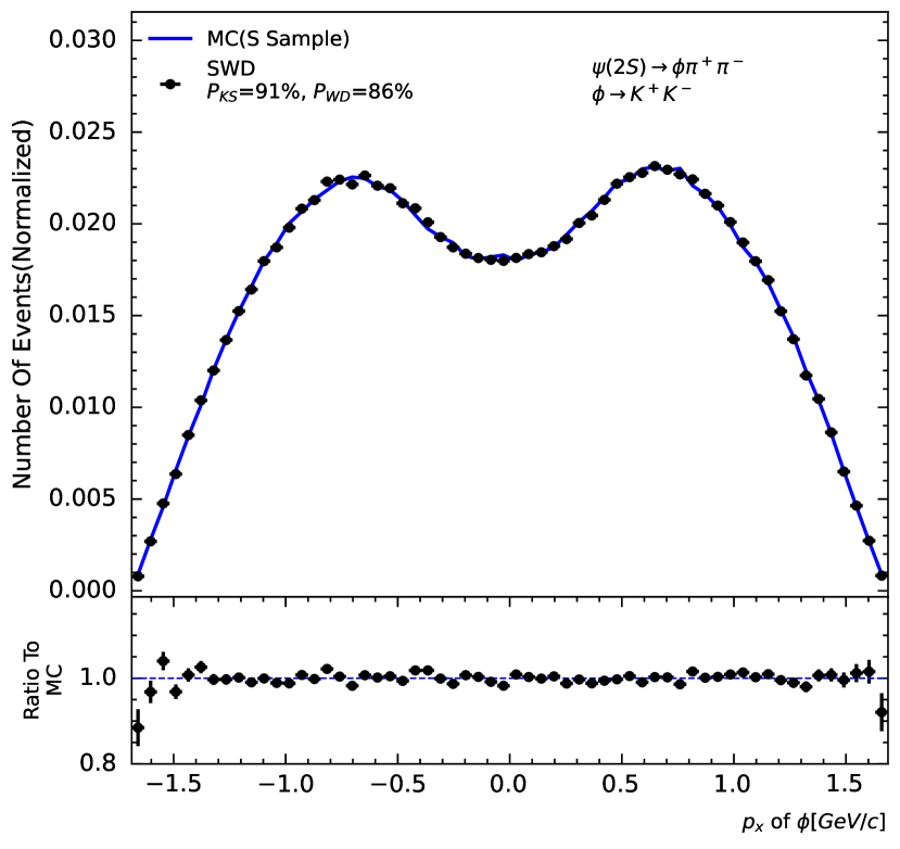
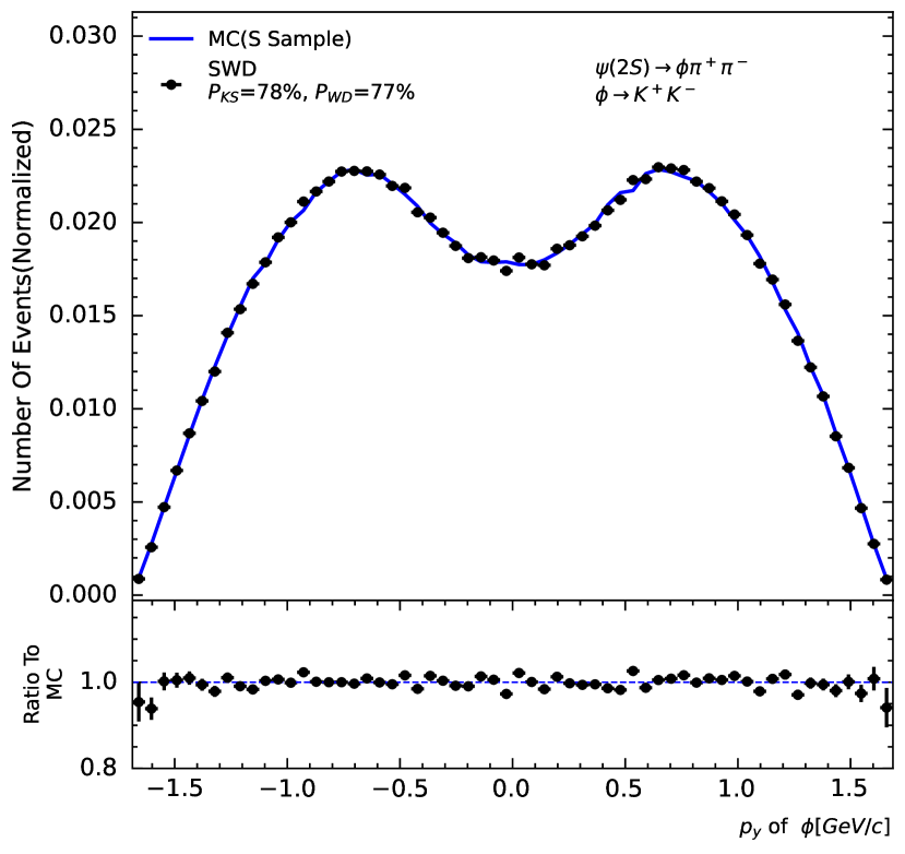
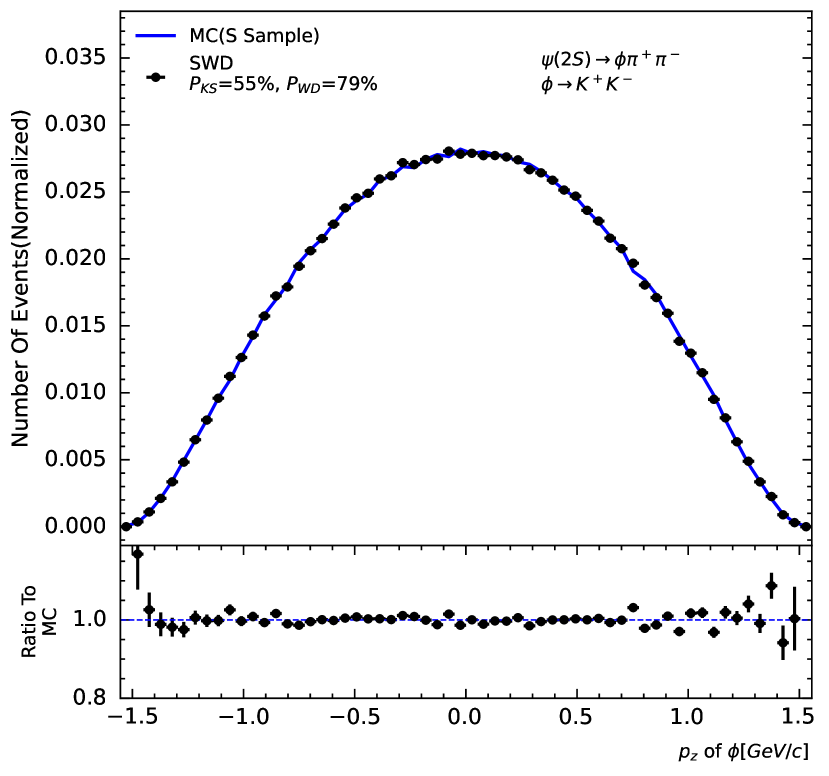
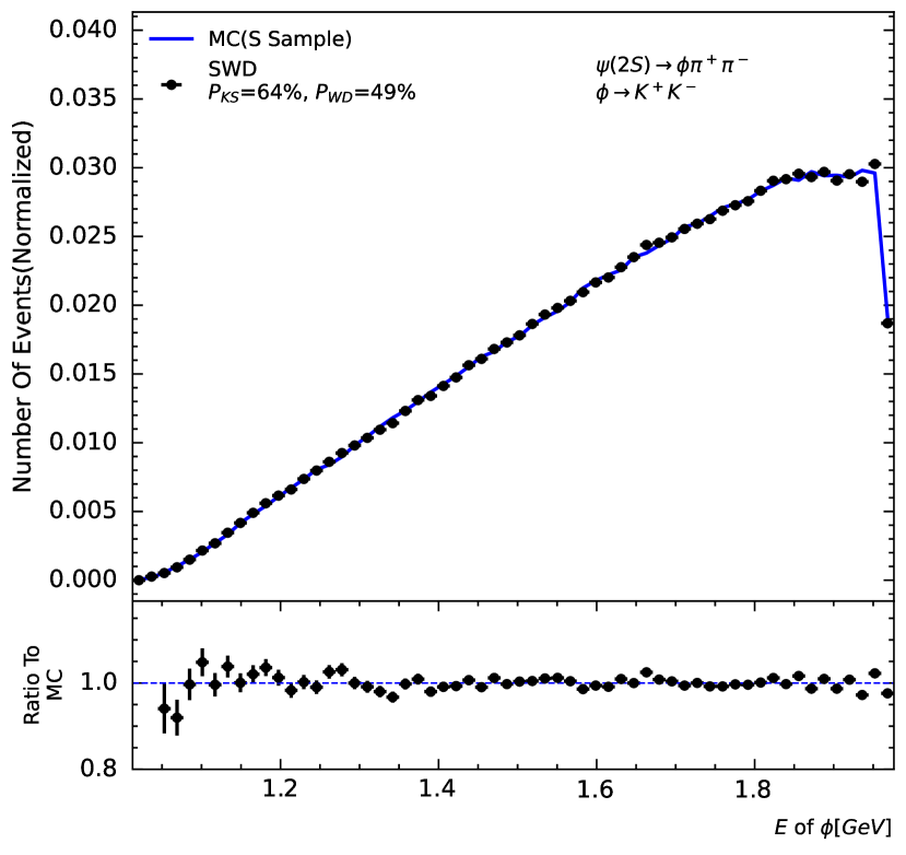
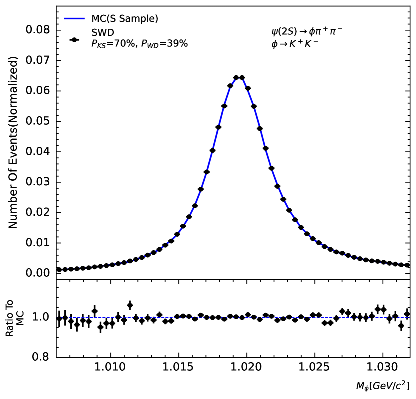
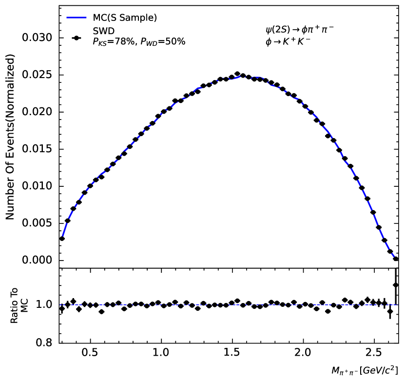
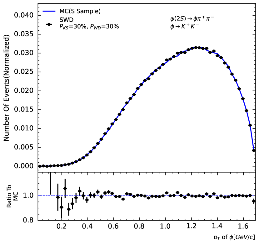
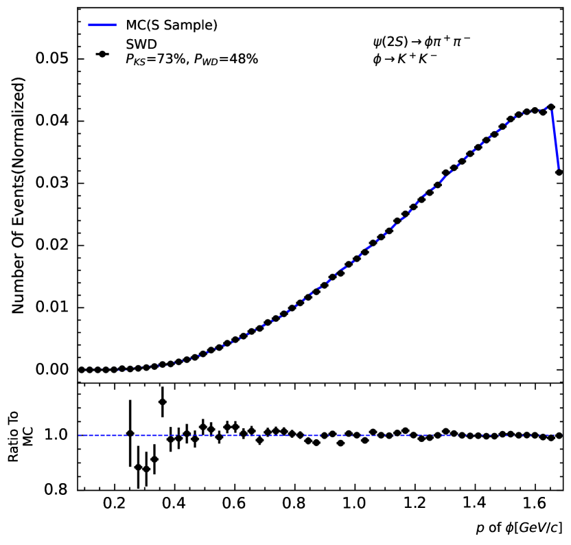
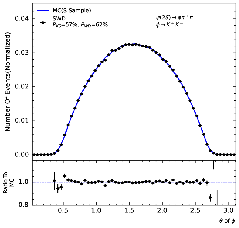
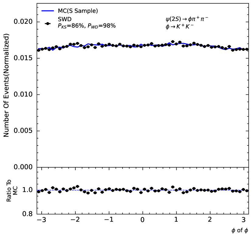
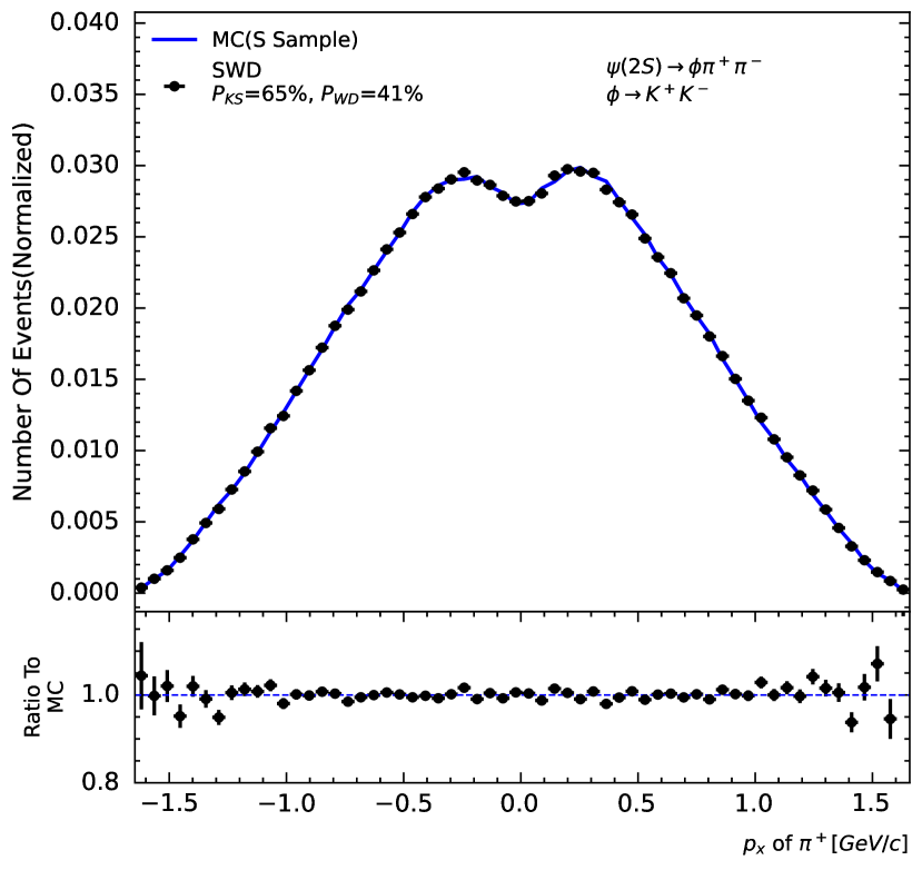
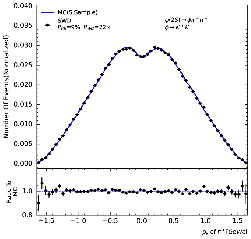
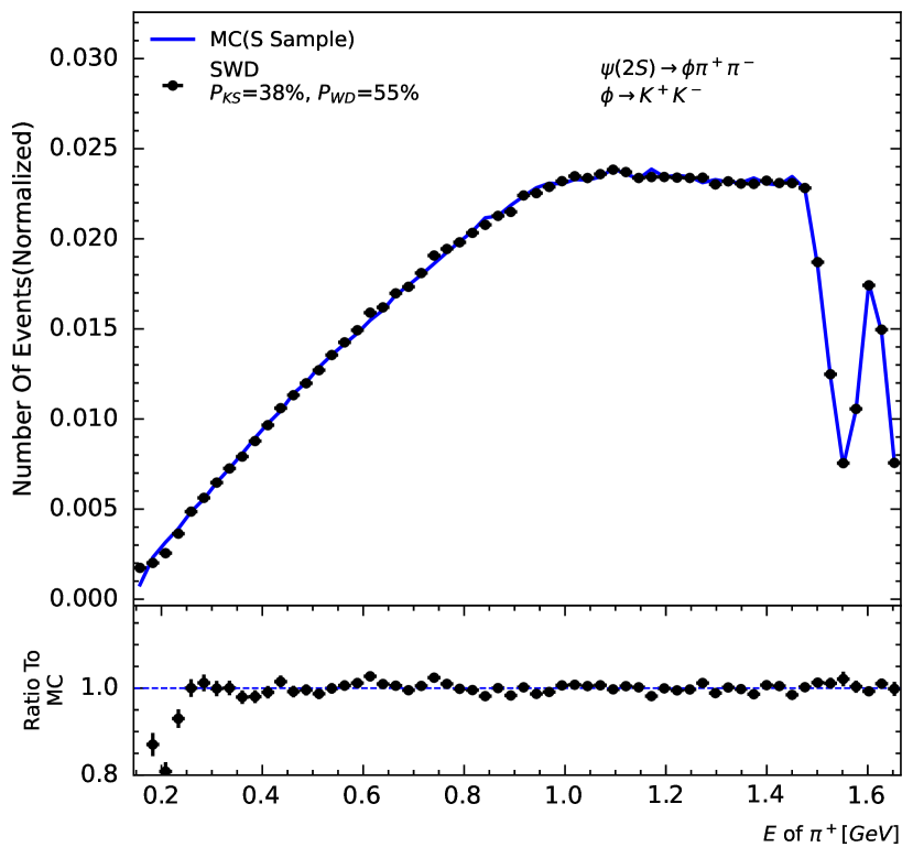
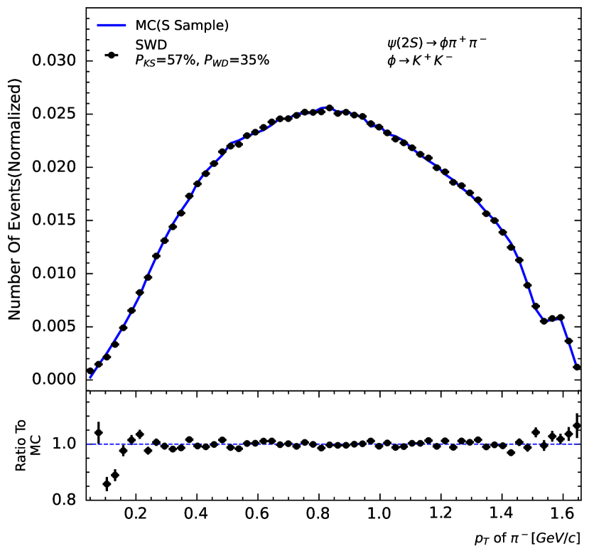
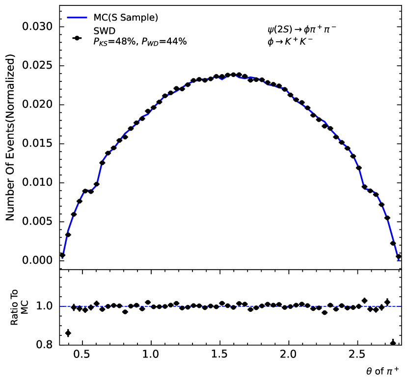
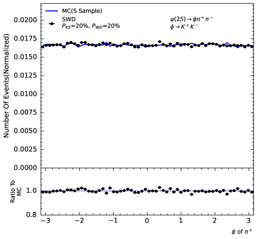
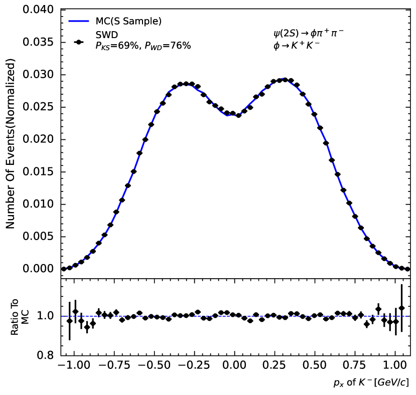
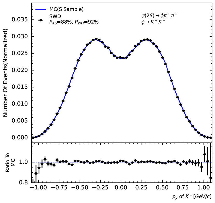
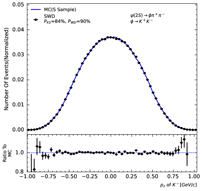
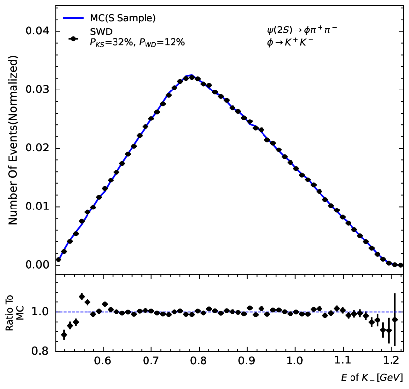
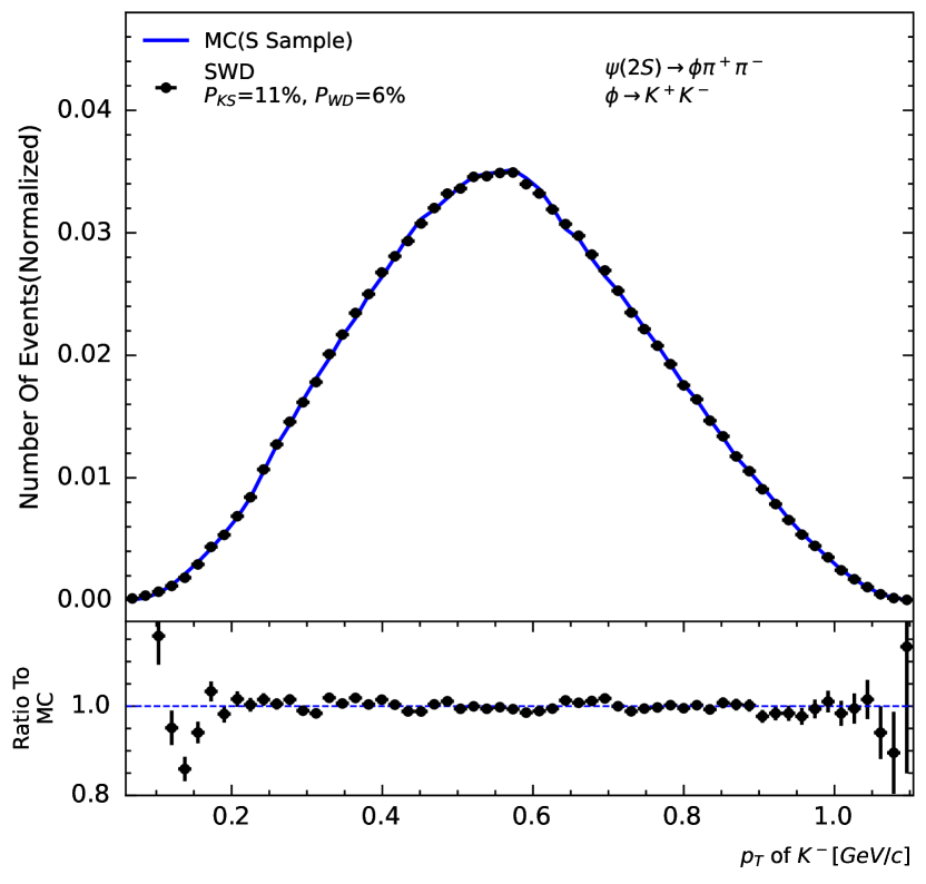
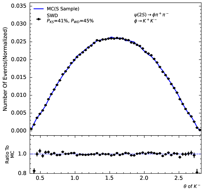
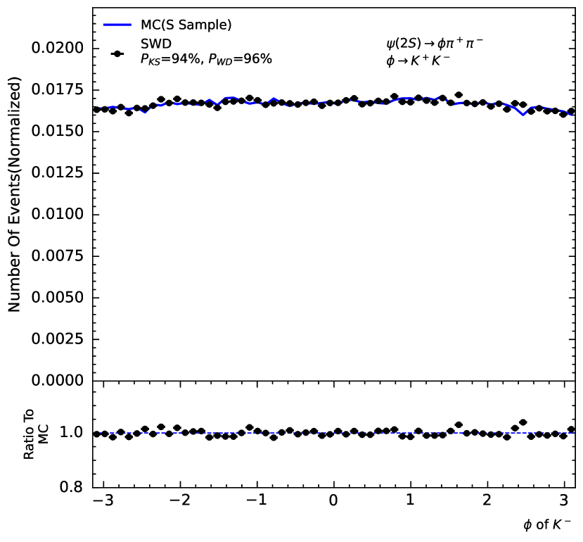
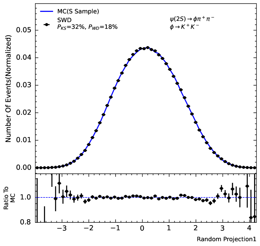
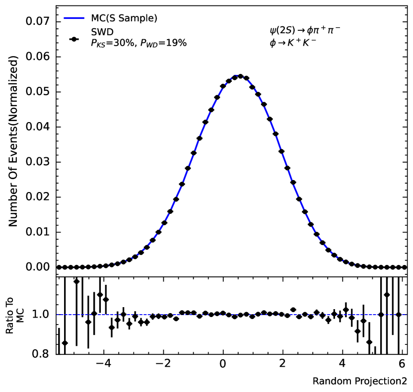
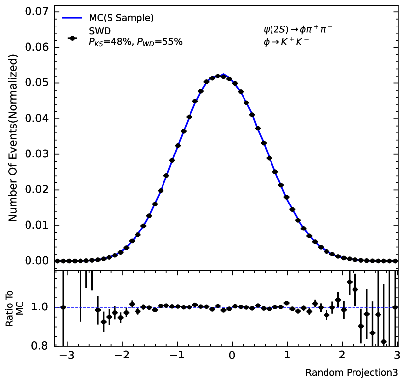
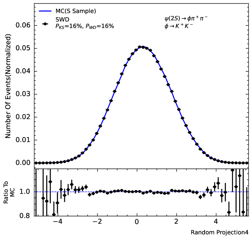
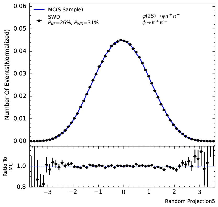
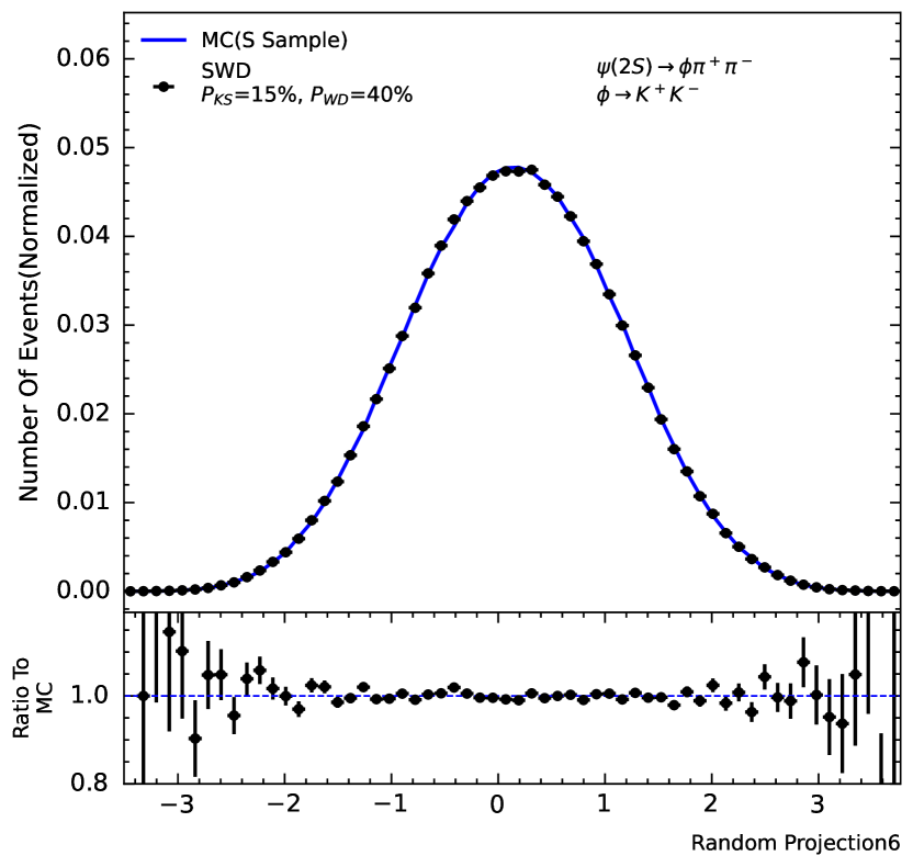
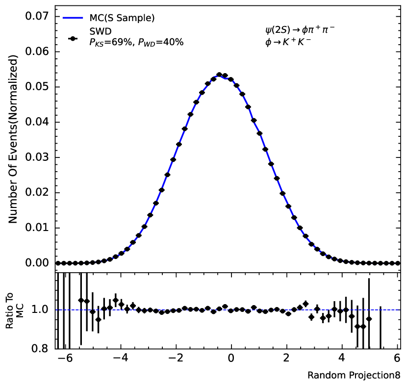
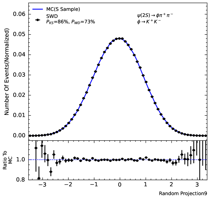
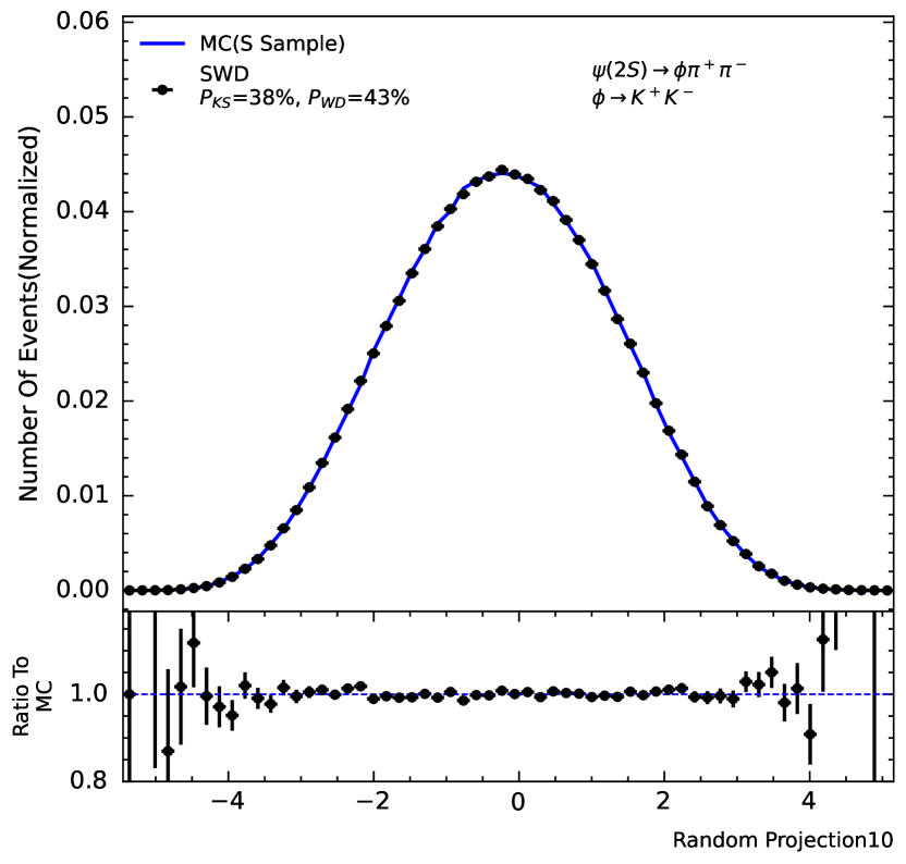
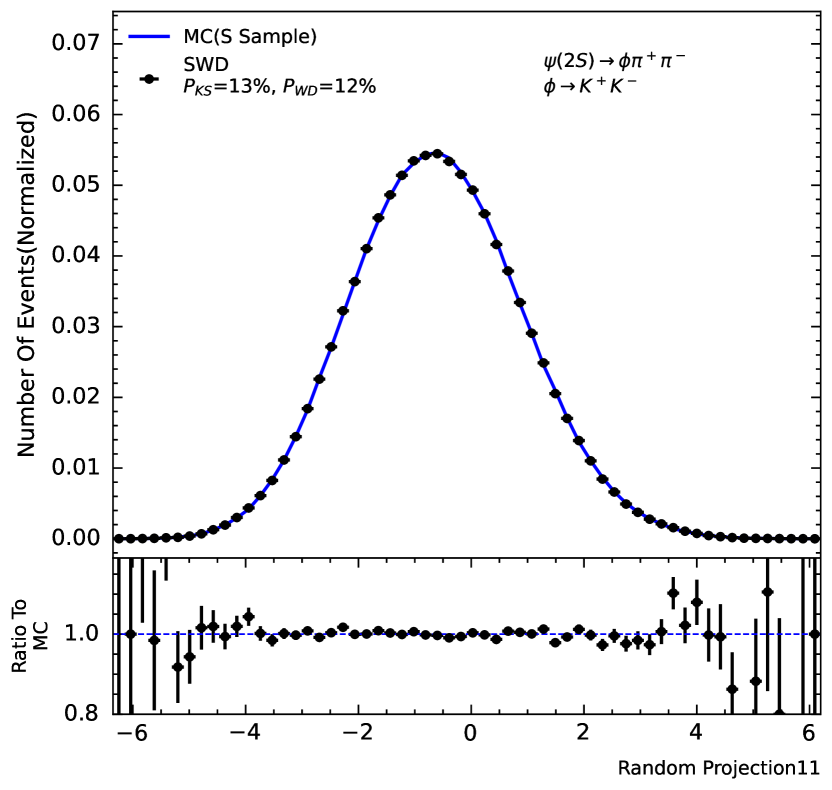
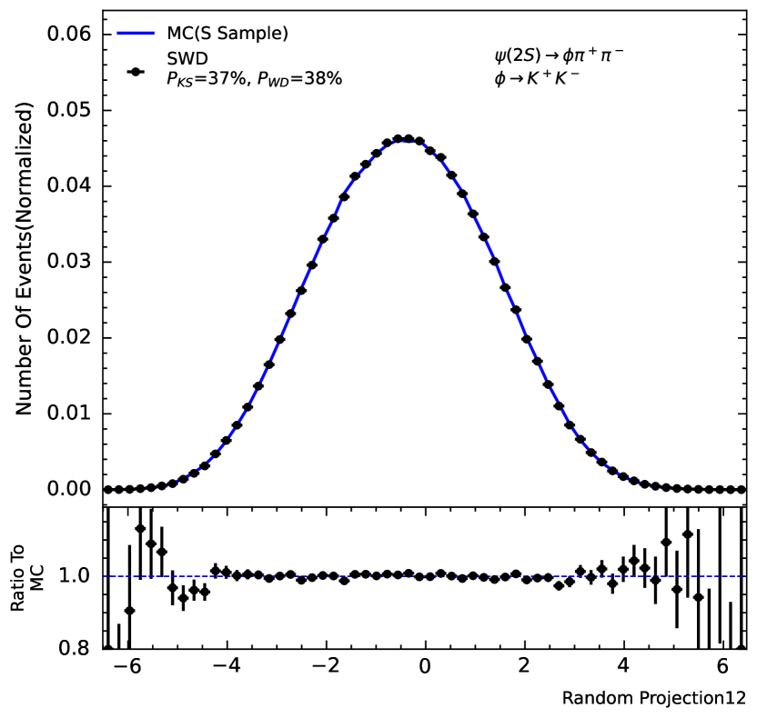
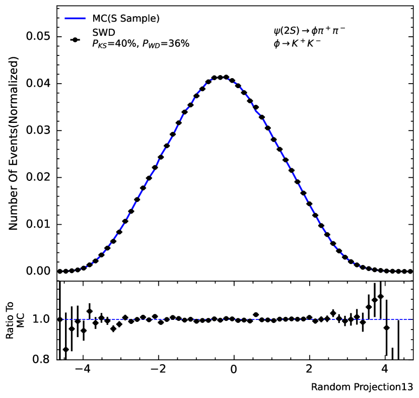
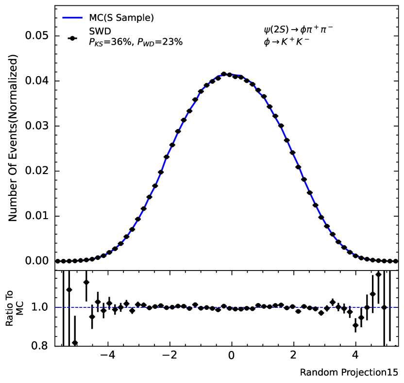
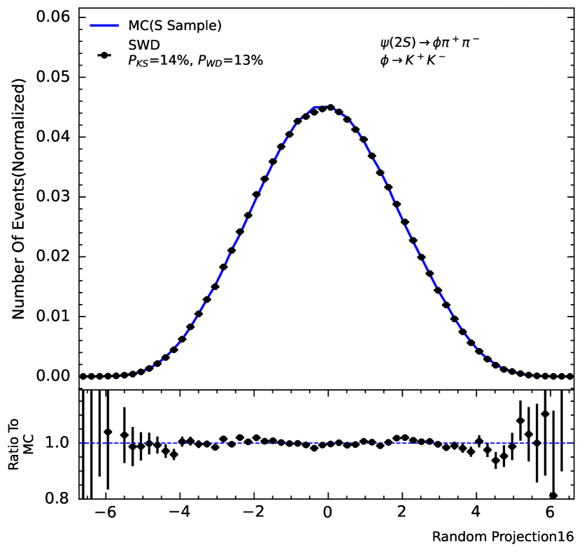
Data comparison was conducted through histograms to intuitively understand the similarity in distribution shape between the data generated by SWD and the Monte Carlo test set data. In Fig.1 We found that the distribution shapes of the SWD-generated data and the test set data were basically consistent with extremely small differences. This initial intuitive comparison provided us with a preliminary understanding of the similarity in the distribution of the SWD-generated data. To further verify the consistency of the distribution between the simulated data and the test set data, we used the Kolmogorov-Smirnov (KS) test, a conventional test for one-dimensional data, and the Wasserstein distance (Wd), based on one-dimensional optimal transport, to conduct a one-dimensional same-distribution test. On specific physical quantity dimensions, the confidence results of the KS test and Wd test confirmed that our SWD-generated data and the test set data have high consistency in the distribution on these dimensions. To comprehensively evaluate the performance of our SWD-generated data, we not only conducted tests on specific physical quantity dimensions but also conducted random one-dimensional linear projections on the free quantities, ignoring factors such as dimensions. This dimensionality reduction technique allows us to simplify high-dimensional data and observe and test the correlation of various distributions in a more intuitive way. Fig.2 shows that even under these projections, the simulated data we generated still maintain a high consistency with the target data. When the training data is 0.25 million, it can be compared with the test set of the order of 1 million under these traditional histogram comparison tests, and it is difficult to see significant differences clearly.

To accurately assess the differences between high-dimensional distributions, we combined the Sliced Wasserstein Distance (SWD) and permutation test methods. Firstly, for two high-dimensional distributions $X$ and $Y$, the original distance ($D_{\text{original}}$) between them is calculated using the Sliced Wasserstein Distance technique. To create a reference distribution, we merged the datasets $X$ and $Y$ and randomly reorganized them multiple times to generate a series of new data pairs ($X_{i}^{\prime}$, $Y_{i}^{\prime}$), noting that this reorganization is not based on the original grouping labels. Subsequently, for each pair of newly matched datasets $X_{i}^{\prime}$ and $Y_{i}^{\prime}$, we calculate the SWD between them to obtain a series of permutation distances ($D_{\text{perm}_{1}}$, $D_{\text{perm}_{2}}$, …, $D_{\text{perm}_{n}}$). In the evaluation process, we compare the position of the original distance ($D_{\text{original}}$) in these permutation distances. As an instance, if $D_{\text{original}}$ is greater than 95% of the $D_{\text{perm}_{i}}$ distances, a p-value of 0.05 can be obtained. In summary, by combining the Sliced Wasserstein Distance with the permutation test, we provide a statistically rigorous and computationally efficient method for assessing the differences between high-dimensional distributions, and for the projection dimensions with specific physical meanings, we can also obtain confidence through the same method. As Fig. 3 shown, this indicator allows us to more accurately quantify the differences in model performance under different parameter settings, describing whether two high-dimensional data are of the same distribution in a situation where the overall high-dimensional confidence cannot be accurately described by the previous histogram comparison. This allows us to further test the degree of compliance of our high-dimensional data and demonstrate the impact on our final model performance under different parameters.

Figure 3: Permutation Test We illustrate the permutation test distribution. The null hypothesis posits that the two samples originate from identical distributions. The p-value can be approximated by the ratio of distances within the permutation groups that exceed the original distance. In the left figure, the null hypothesis cannot be rejected due to its p-value of 26.6 % when the training size is 1.8 million. However, in the right figure, the null hypothesis can be rejected given that the p-value is 0 % when the training size is 50,000. [35]

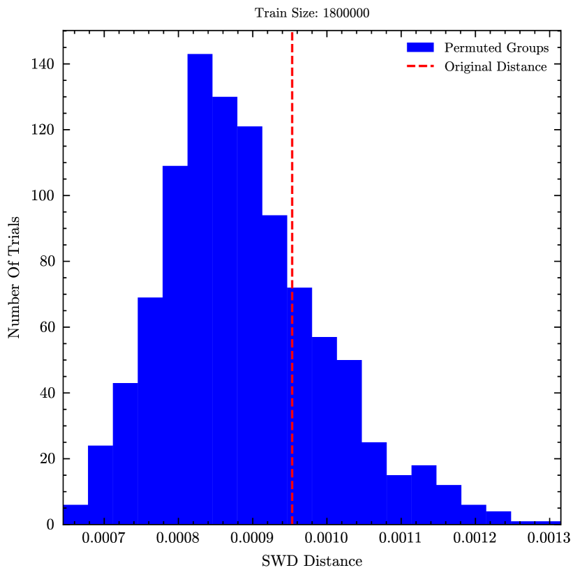
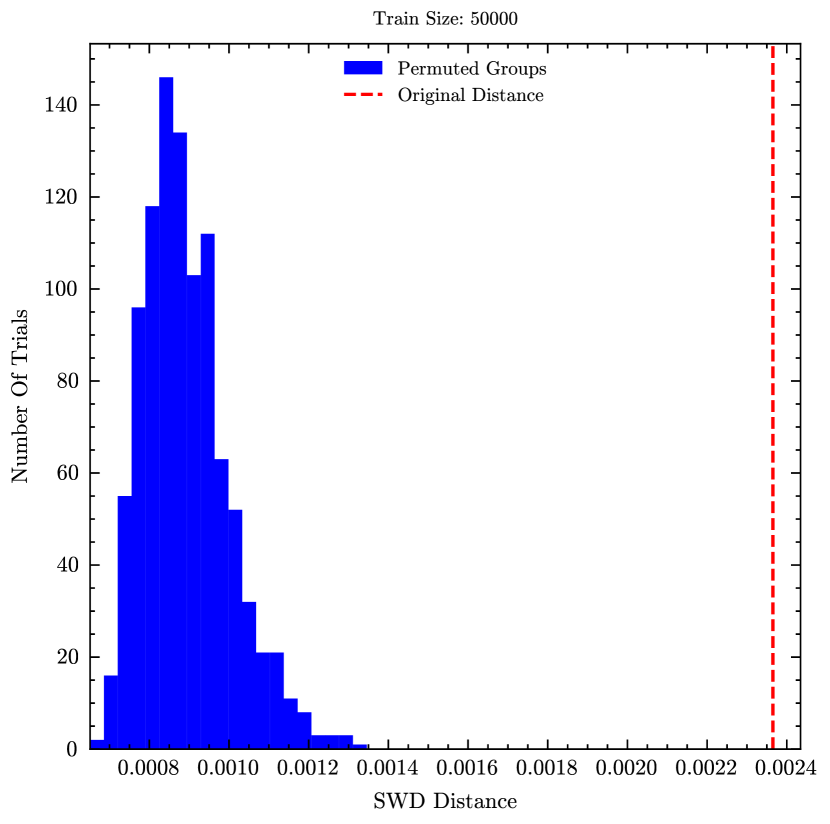
Table 1 shows the impact of the number of training data and batch size on model performance. We found that larger data volumes are beneficial for model learning, but when the data exceeds a certain amount, increasing the data may not significantly improve model learning, but it may produce better results when facing larger test data sets. We explore the impact of different batch sizes on model performance. Because our training strategy is different from conventional deep learning training, the larger the batch size, the more accurate the loss sorting match will be when calculating the loss. In principle, the smaller the batch size, the greater the impact of sample sampling. As shown in the table, a too small batch size will greatly discount the model performance, but when the batch size is increased to a certain extent under our existing data volume, it will balance in the loss sorting match and model training, and there are no obvious gains in further increasing it.

Table 1: The impact of the number of train data and batch size

The number of train data	batch size	swd test distance	swd test p value	wd test distance	wd test p value
1800000	16	0.0013275146	0%	0.0011272430	38.1%
1800000	32	0.0013179779	0.1%	0.0012664795	15.6%
1800000	64	0.0010271072	10.9%	0.0010070801	65.2%
1800000	128	0.0009021759	41.6%	0.0009355545	85.0%
1800000	256	0.0009551048	26.6%	0.0009689331	77.5%
1800000	512	0.0010681152	6.1%	0.0012102127	22.5%
1500000	256	0.0008893013	45.3%	0.0010929108	43.6%
1250000	256	0.0010309219	11.1%	0.0011281967	39.1%
1000000	256	0.0009355545	27.9%	0.0011348724	33.4%
750000	256	0.0010538101	7.4%	0.0012331009	18.5%
500000	256	0.0012292862	0.7%	0.0014400482	4.4%
250000	128	0.0015182495	0%	0.0019493103	0%
100000	64	0.0015773773	0%	0.0019092560	0%
50000	32	0.0023670197	0%	0.0029506683	0%

In Table 2, we discuss the impact of different gamma values on model performance. A reasonable gamma value can fine-tune the constraints of a single dimension, which can be seen as an optimization of the original SWD, and it is beneficial to the overall effect of the model. However, if the gamma value is too large, the model may be too inclined to learn some specific physical quantity dimensions and ignore the overall characteristics of the high-dimensional data distribution.

Table 2: The impact of $\gamma$

$\gamma$	swd test distance	swd test p value	wd test distance	wd test p value
0	0.0010623932	5.6%	0.0036334991	0%
0.1	0.0009551048	26.6%	0.0009689331	77.5%
1	0.0014295578	0.1%	0.0010690689	50.3%

In summary, these results provide us with important guidance on how to adjust model parameters to optimize performance. Specifically, we need to ensure sufficient training data volume and enough batch size to reduce disturbances, to ensure that the generated data is consistent with the target distribution, and a reasonable gamma value to ensure that the model can balance the learning of specific physical quantity dimensions and the overall characteristics of high-dimensional data.

3 Discussion

In this section, we will discuss the universal training methods and model testing methods in the machine learning generative models for future high-energy physics experiment events.

Strong Physical Constraints In high-dimensional data, due to its inherent characteristics, there exist some strong constraint conditions. For example, the mass of each final-state particle is fixed after particle identification, which is a strong constraint  [36, 37]. Another example is that when using Phikk data, we boost the data to the center-of-mass system, which results in the sum of the three momenta of the final-state particles must be zero, this is also a strong constraint. Moreover, some physical quantities have describable ranges, and if they exceed this range, they do not comply with physical laws. In previous research, these strong constraints are often assumed to be content that the model needs to learn autonomously, and are regarded as evidence that deep learning can be used to learn physical knowledge. However, although we can obtain an approximate relationship in this way, there are often a certain number of deviating values. This is unreasonable for actual physical analysis, because these strong constraints are the basic characteristics of physical phenomena and should not be ignored or approximated. Therefore, we advocate taking these basic dynamical relationships as our prior knowledge, allowing the model to only need to learn the degrees of freedom in the dynamics. Then, we can use this prior physical knowledge to solve and obtain all the physical quantities we finally need. In this way, we can describe physical phenomena more accurately and avoid the bias caused by ignoring strong constraints. At the same time, these degrees of freedom will be scaled to -1 to 1 according to the prior range, to fit the commonly used output function tanh in deep learning [38]. Using our method, we can not only ensure that the model generates data in accordance with basic physical laws, but also make the model more focused on learning the physical distribution. For some sharp-shaped degrees of freedom such as mass spectra, we can use the sinh-arcsinh distribution transformation to transform them to be smoother [39]. This method combines the prior knowledge of physics with the learning process of the deep learning model, ensuring the physical rationality of the model and improving the learning efficiency of the model.

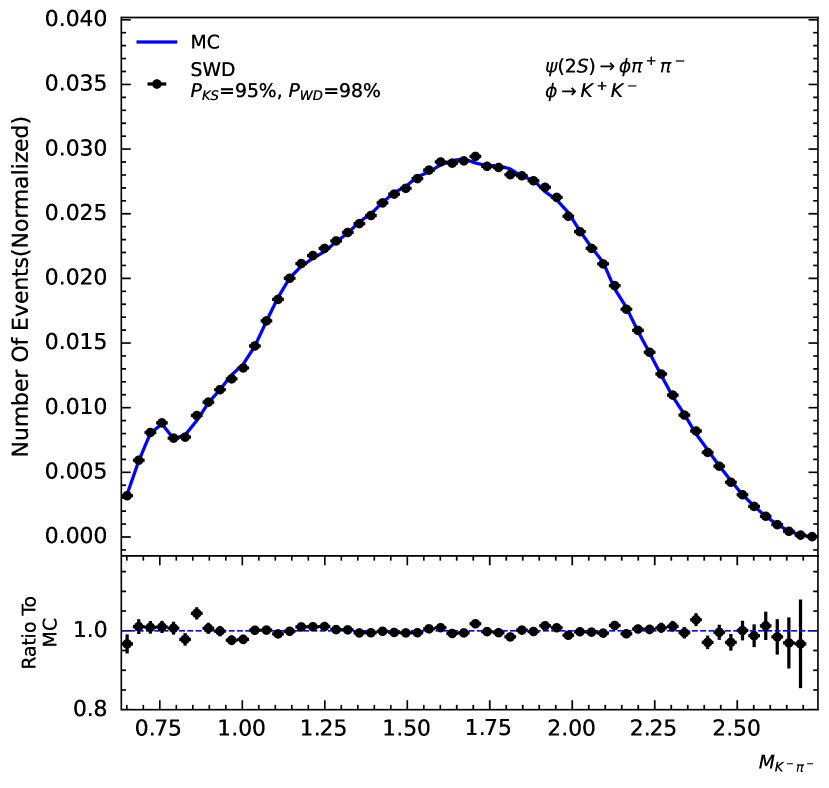
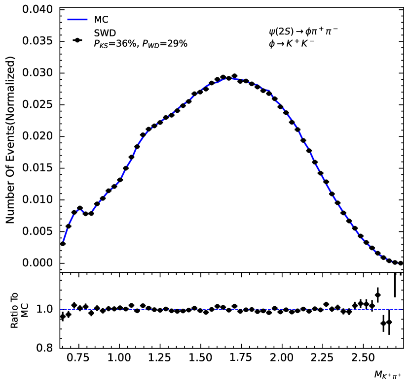
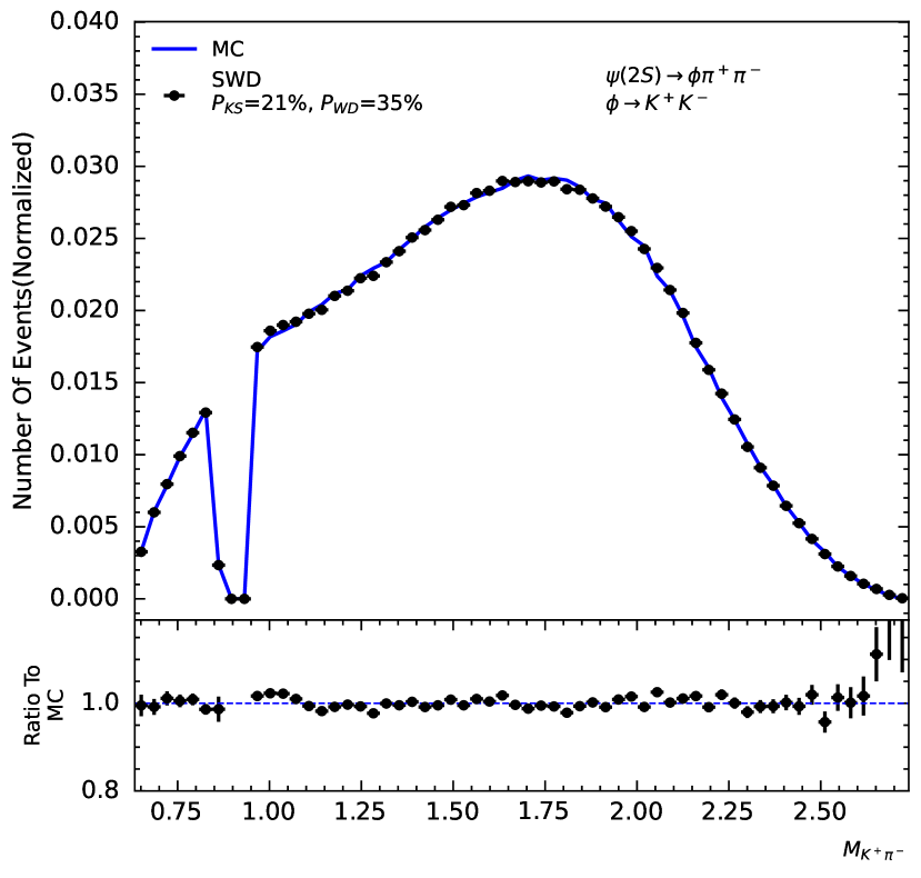
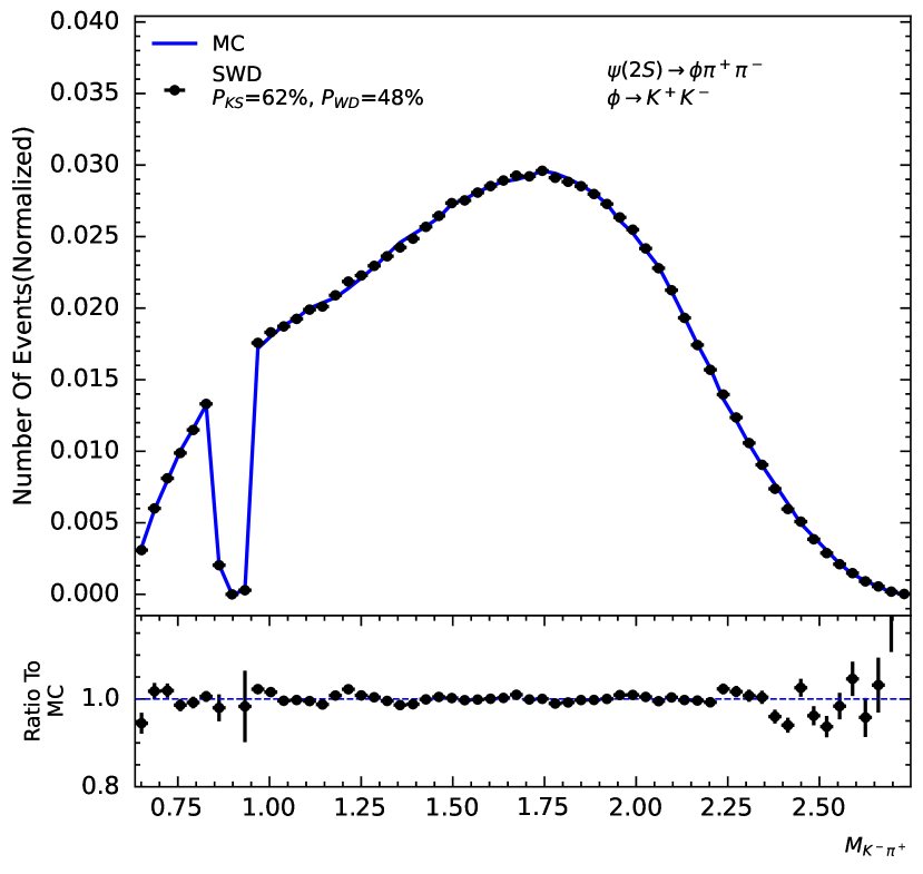
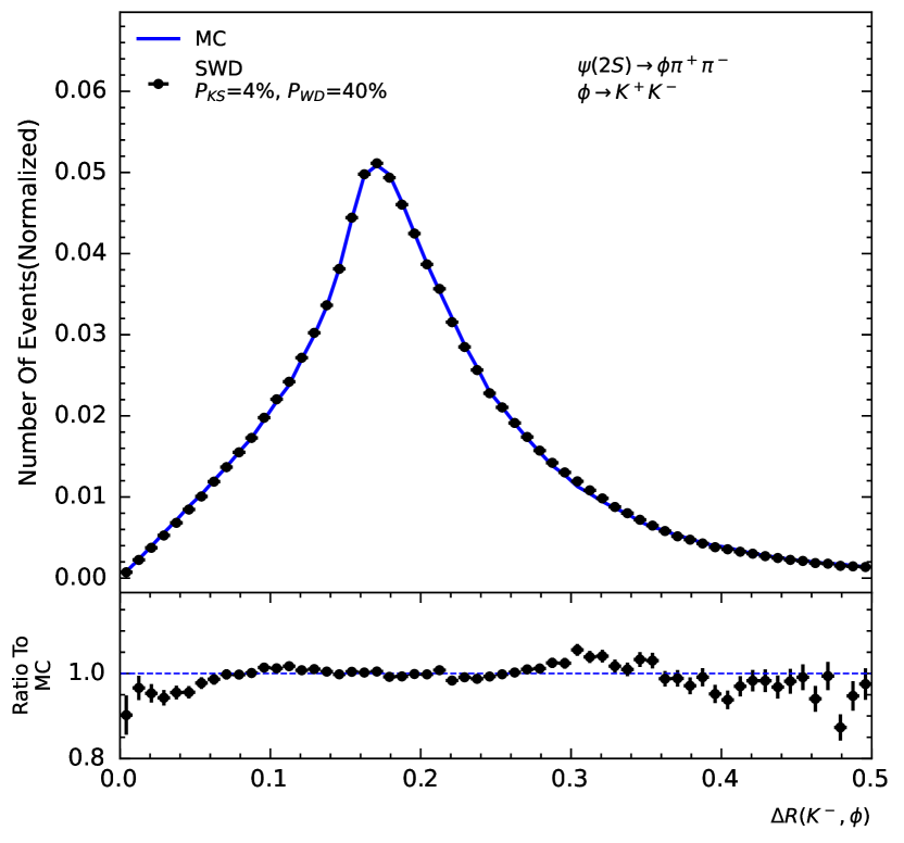
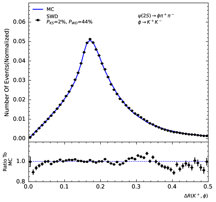
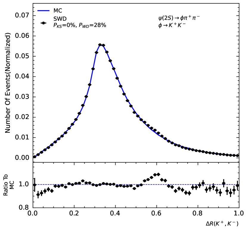
Detector Effects In particle physics research, the detection and analysis of high-dimensional continuous distributions is a complex task. Due to the complexity of detector effects, high-dimensional distributions may exhibit non-smooth or spatial defect characteristics. These characteristics are caused by factors such as the geometric shape, sensitivity, and calibration errors of the detector, such as the theta angle distribution and transverse momentum (pt) distribution of particles [40, 41]. Meanwhile, in high-energy physics experiments, veto operations are used to reduce background signals to enhance the distinction between signals and backgrounds. However, this operation may directly cause a part of the high-dimensional data to be missing, which may introduce bias and efficiency loss. Although SWD can easily handle generated continuous high-dimensional distributions, under the influence of detector efficiency, due to its initial function nature, the learning process may become difficult and inefficient. These issues bring additional complexity to our model training, but also provide us with opportunities to test the performance of the model in handling complex high-dimensional distributions. To fully understand and let the model learn these distributions, it may be necessary to comprehensively consider the complex interactions of experiments, data processing, and statistical methods, and take appropriate correction and calibration measures. We can adopt some strategies, such as additional learning for physical quantities that are highly affected by detector efficiency. Through such corrections, we can adjust the entire high-dimensional distribution to better understand and describe the intrinsic structure of experimental data. And we use a parameter as the proportion of the correction term, we find that taking an appropriate parameter can make a fine-tuning of the original high-dimensional distribution, so that the data can learn the true high-dimensional data distribution. From the dimensions of physical quantities in Fig. 4 hat have not been put into additional constraints, we do not think that it is just an enhancement of some additional physical quantities, but the entire high-dimensional data can benefit.

Figure 4: 1D Histograms of the extra projection distributions We show the distribution with physical meaning but without WD constraints. We can see it still holds high agreement with target distribution.

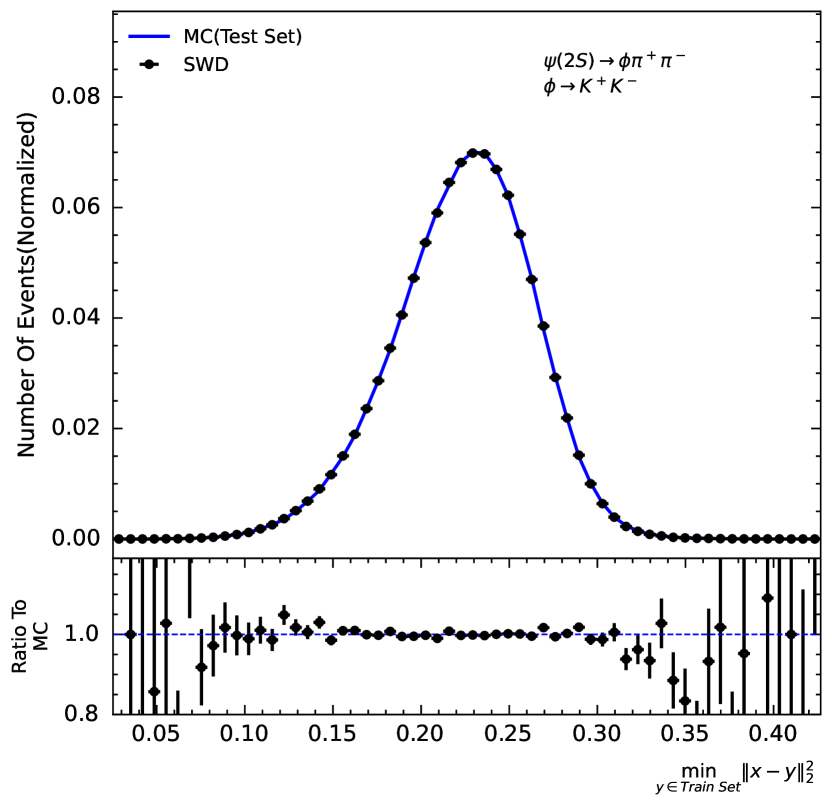
Measuring Overfitting When the model is overly complex, it may lead to the model understanding the characteristics of the training dataset too deeply, so that it merely replicates the training dataset, instead of learning the entire high-dimensional data distribution. If overfitting occurs, the data generated by the model may be a subset of the training set, and the generalization ability of the model will be greatly reduced. Therefore, in our research, we need to ensure that our generated simulated data do not simply replicate the training data, but learn its distribution and generate new data based on this distribution. To test whether our simulated data have overfitted, we adopted a test method based on the minimum Euclidean distance. We calculated the minimum Euclidean distance from each data point in the test set to all data points in the training set, and conducted statistics on these distances. Then, we compared this statistical distribution with the statistical distribution of the minimum Euclidean distance from the simulated data generated by Sliced Wasserstein Distance (SWD) to all data in the training set. If our SWD model is overfitting, then we would expect to see that the minimum distance between the simulated data and the training set is significantly smaller than the minimum distance between each data point in the test set and the training set. However, our results in Fig.5 show that the simulated data generated by SWD do not significantly bias towards the training set data, but are very similar to the minimum distance distribution from the test set to the training set data. This indicates that our model did not simply replicate the training data, but learned its distribution and successfully generated new data based on this distribution. Therefore, we conclude that our simulated data generated by SWD successfully avoided the problem of overfitting, and the distribution properties of its generated data are almost the same as those of the new data generated by the same use of Monte Carlo simulation. This result further proves the effectiveness and reliability of our simulation method.

Figure 5: 1D Histograms of the minimum distance We show the distribution of minimum distance between train data and test data / our generated data. We can see our generated samples have high novelty even like the new generated MC data.

4 Method

Monte Carlo Data We use the BES III simulation framework to simulate phase-space Monte Carlo, where $\psi(2S)$ is produced in electron-positron collisions and subsequently decays into $\phi$, $\pi^{+}$, $\pi^{-}$, with $\phi$ finally decaying into $K^{+}$, $K^{-}$. Our data is boosted into the center-of-mass system of $\psi(2S)$, hence we have a total of eight degrees of freedom. We selected $M_{\phi}$, $M_{\pi^{+}\pi^{-}}$, $\theta_{\phi}$, $\phi_{\phi}$, as well as $\theta$ and $\phi$ of the decayed $K^{+}$, $K^{-}$ in the rest frame of $\phi$, and the same applies to the rest frame of $\pi^{+}\pi^{-}$ [42]. Note that this does not mean that $\psi(2S)$ directly decays into a resonance state of $\phi$ and $\pi^{+}\pi^{-}$, but refers to the dynamical variables in the rest frame of $\pi^{+}\pi^{-}$. For training, we need to record the variable range of the Monte Carlo data. For the final-state particles, we determine their $\theta$ range affected by the detector acceptance based on the data. For the mass of $\phi$, we select $1.006<M_{\phi}<1.032$. For $K^{+}\pi^{-}$ and $K^{-}\pi^{+}$, we have $M_{K\pi}<0.85$, $M_{K\pi}>0.95$ to remove possible $K^{*}$ decay events.

SWD Theory Optimal Transport is a theory in the field of mathematics that studies how to transfer matter from one distribution to another with the minimum cost. Optimal Transport theory is now applied in multiple fields, including image processing, machine learning, economics, etc [43]. In the Optimal Transport problem, we need to define a cost function $c(x,y)$ that represents the cost of transferring from point x to point y. The Optimal Transport problem is to find a transfer (or coupling) of probability measures $\pi$ that minimizes the total transfer cost, i.e., minimizes $\int c(x,y)d\pi(x,y)$. In many cases, the cost function $c(x,y)$ is set to some power of the distance between x and y. The Optimal Transport distance (or Wasserstein distance) is a way to measure the distance between two probability distributions. Given two probability distributions P and Q, their Wasserstein distance is defined as the cost of the probability measure that achieves the minimum total transfer cost [44].

Sliced Wasserstein Distance (SWD) is a variant of the Wasserstein distance, which transforms the high-dimensional Optimal Transport problem into a one-dimensional problem for ease of computation. Specifically, for each randomly chosen direction, SWD projects the distribution onto this direction and then calculates the Wasserstein distance of these one-dimensional distributions. This process is repeated multiple times and the results are averaged to obtain the final distance estimate. First, let us define the one-dimensional Wasserstein distance. For the one-dimensional case, the Wasserstein distance between two distributions $P$ and $Q$ can be defined as the L1 distance between their cumulative distribution functions (CDFs) [45], i.e.,

$$WD(P,Q)=\int|F_{P(x)}-F_{Q(x)}|dx$$

where $F_{P}$ and $F_{Q}$ are the cumulative distribution functions of distributions $P$ and $Q$. For the high-dimensional case, the Sliced Wasserstein Distance is defined through the integral of the one-dimensional Wasserstein distance:

$$SWD(P,Q)=\int WD(P_{\theta},Q_{\theta})d\theta$$

where $P_{\theta}$ and $Q_{\theta}$ are the one-dimensional distributions of distributions P and Q projected onto direction $\theta$. $\theta$ is a direction randomly drawn from a uniform distribution. $W(P_{\theta},Q_{\theta})$ is the Wasserstein distance between these two one-dimensional distributions. Note that the integral here is over all possible directions $\theta$, i.e., in practice, we usually approximate this integral by sampling a large number of random directions and taking the average. It should be noted that the formula here is for the case of continuous probability distributions. For the discrete case, we assume that we have two sets of points $X={x_{1},...,x_{n}}$ and $Y={y_{1},...,y_{n}}$, each set is in $R^{d}$. We can define the one-dimensional discrete Wasserstein distance as:

$$WD(X_{\theta},Y_{\theta})=\frac{1}{n}\sum_{i=0}^{n}x_{i\theta}-y_{\pi(i)\theta}$$

where $X_{\theta}$ and $Y_{\theta}$ are the projections of X and Y in direction $\theta$, and $\pi$ is a permutation that minimizes the above sum. In the one-dimensional case, such $\pi$ can be found by sorting the points after projection. This is because in one dimension, the optimal transport scheme is to pair each point $x_{i\theta}$ with its immediate neighbor $y_{\pi(i)\theta}$. Then, the Sliced Wasserstein Distance for the discrete case is defined as

$$SWD(X,Y)=E[WD(X_{\theta},Y_{\theta})]$$

The expectation is calculated by sampling along multiple random directions $\theta$. We choose the projection dimension in the unit circle, which can make the projection more uniform [46], and then calculate and average the one-dimensional Wasserstein distances in these directions [23, 44]. Some revised theories regarding the Sliced Wasserstein Distance have been proposed to better accommodate complex high-dimensional data. These modifications have potential applications in event generation in the future work [47] [48] [49] [50].

To correct for detector effects and the spatial defects in high-dimensional data caused by event selection, we will make additional corrections to the dimensions of specific physical quantities, so our total loss is

$$Loss=SWD(X,Y)+\gamma\cdot E[WD(X_{\theta_{specific}},Y_{\theta_{specific}})]$$

Figure 6: Model Overview We input the random samples from uniform distribution, non-linearly expand it, split into desired tokens and feed it into a standard Transformer encoder to learn correlation of multi-variable distribution. Finally we can generate the reasonable high dimensional data

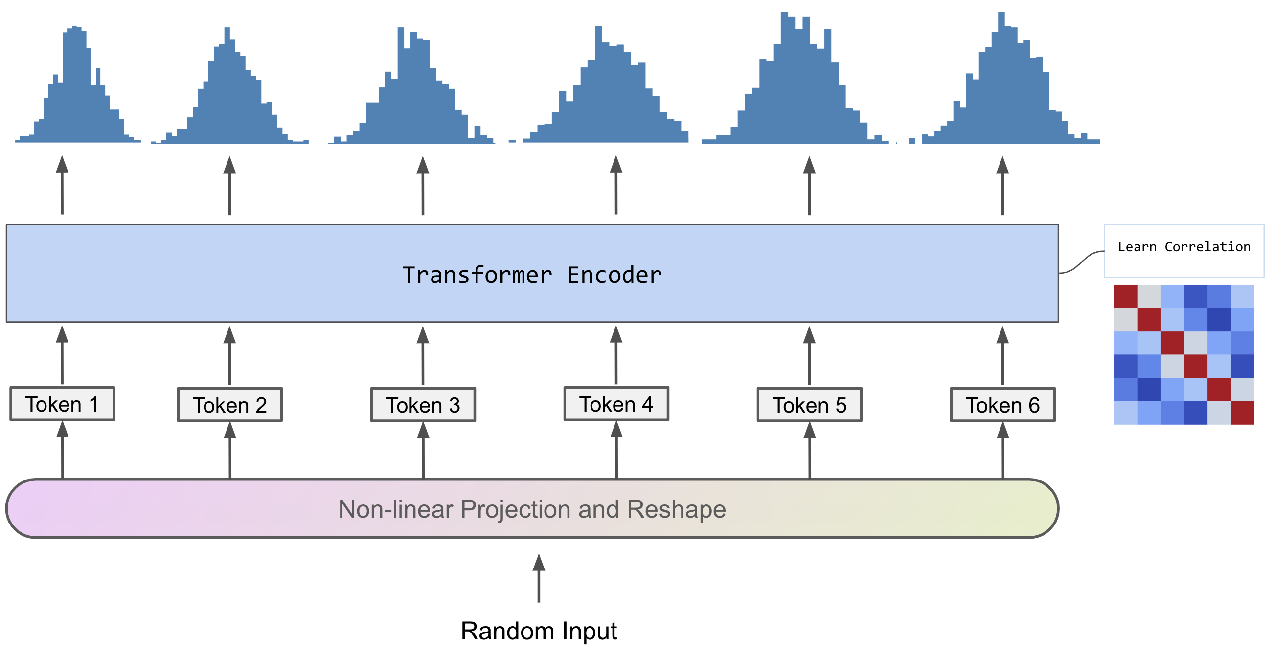
Model Training We employ the Transformer model, which is based on the self-attention mechanism [30]. This mechanism allows the model to compute a weight of relationships for each token in the input sequence [51], enabling the model to capture the interrelationships within high-dimensional data. This model is designed to learn and generate complex high-dimensional data. Initially, after inputting a latent vector uniformly distributed from -1 to 1, we project it to a vector of the number of degrees of freedom x 1024, and reshape it into desired tokens as Fig.6 shown. Each individual token represents an independent unit distribution. This process is akin to breaking down a sentence into words or morphemes in natural language processing. On this basis, we consider a complex multivariate distribution as a sequence of these unit distribution tokens. Each token will contain 1024 elements, which also means that a token has information of 1024 points in that dimension. We then feed these tokens into a Transformer model. The core of the Transformer model is its self-attention mechanism. This mechanism can handle high-dimensional data and can calculate the complex interactions and dependencies of each distribution to the others. This capability allows us to have a global and in-depth understanding of the multivariate distribution. We use the trained Transformer model to predict or generate new multivariate distributions. Since the Transformer model can comprehend the complex relationships among these distributions, it is capable of generating multivariate distributions that meet expectations.

5 Code Available

The code used for the analysis and visualizations in this study is openly available for the research community. We believe in open science and therefore, we have made our code publicly accessible. This allows other researchers to reproduce our results, use our code as a base for their own research, and facilitate further development and improvements. The code, data and results can be found at our GitHub repository: https://github.com/caihao/SWD-EvtGen. In case of any queries or issues related to the code, feel free to raise an issue on the GitHub repository or contact us directly. We will do our best to assist and support your research endeavors.

6 Acknowledgements

The National Science Foundation of China(nos. 11735010, U1932108, U2032102 and 12061131006) provided the funding for this project. Their financial support was instrumental in the realization of our research goals. The numerical calculations in this paper have been done on the supercomputing system in the Supercomputing Center of Wuhan University.

7 Competing Interests

The authors declare that they have no competing interests.

References

- \bibcommenthead
- Seymour and Marx [2013] Seymour, M.H., Marx, M.: Monte Carlo Event Generators (2013)
- and Andrea Valassi et al. [2021] Andrea Valassi, Yazgan, E., McFayden, J., Amoroso, S., Bendavid, J., Buckley, A., Cacciari, M., Childers, T., Ciulli, V., Frederix, R., Frixione, S., Giuli, F., Grohsjean, A., Gütschow, C., Höche, S., Hopkins, W., Ilten, P., Konstantinov, D., Krauss, F., Li, Q., Lönnblad, L., Maltoni, F., Mangano, M., Marshall, Z., Mattelaer, O., Menendez, J.F., Mrenna, S., Muralidharan, S., Neumann, T., Plätzer, S., Prestel, S., Roiser, S., Schönherr, M., Schulz, H., Schulz, M., Sexton-Kennedy, E., Siegert, F., Siódmok, A., Stewart, G.A.: Challenges in monte carlo event generator software for high-luminosity LHC. Computing and Software for Big Science 5(1) (2021) https://doi.org/10.1007/s41781-021-00055-1
- Bähr et al. [2008] Bähr, M., Gieseke, S., Gigg, M.A., Grellscheid, D., Hamilton, K., Latunde-Dada, O., Plätzer, S., Richardson, P., Seymour, M.H., Sherstnev, A., Webber, B.R.: Herwig++ physics and manual. The European Physical Journal C 58(4), 639–707 (2008) https://doi.org/%****␣sn-article.bbl␣Line␣125␣****10.1140/epjc/s10052-008-0798-9
- Sjöstrand et al. [2015] Sjöstrand, T., Ask, S., Christiansen, J.R., Corke, R., Desai, N., Ilten, P., Mrenna, S., Prestel, S., Rasmussen, C.O., Skands, P.Z.: An introduction to PYTHIA 8.2. Computer Physics Communications 191, 159–177 (2015) https://doi.org/10.1016/j.cpc.2015.01.024
- Bothmann et al. [2019] Bothmann, E., Chahal, G.S., Höche, S., Krause, J., Krauss, F., Kuttimalai, S., Liebschner, S., Napoletano, D., Schönherr, M., Schulz, H., Schumann, S., Siegert, F.: Event generation with sherpa 2.2. SciPost Physics 7(3) (2019) https://doi.org/10.21468/scipostphys.7.3.034
- Jadach et al. [2023] Jadach, S., Ward, B.F.L., Was, Z., Yost, S.A., Siodmok, A.: Multi-photon monte carlo event generator KKMCee for lepton and quark pair production in lepton colliders. Computer Physics Communications 283, 108556 (2023) https://doi.org/10.1016/j.cpc.2022.108556
- Ping [2008] Ping, R.-G.: Event generators at BESIII. Chin. Phys. C 32, 599 (2008) https://doi.org/%****␣sn-article.bbl␣Line␣200␣****10.1088/1674-1137/32/8/001
- de Favereau et al. [2014] Favereau, J., , Delaere, C., Demin, P., Giammanco, A., Lemaître, V., Mertens, A., Selvaggi, M.: DELPHES 3: a modular framework for fast simulation of a generic collider experiment. Journal of High Energy Physics 2014(2) (2014) https://doi.org/10.1007/jhep02(2014)057
- Belyaev et al. [2003] Belyaev, I., Charpentier, P., Easo, S., Mato, P., Palacios, J., Pokorski, W., Ranjard, F., Tilburg, J.: Simulation Application for the LHCb Experiment (2003)
- Aaij et al. [2023] Aaij, R., et al.: Test of lepton flavor universality using B0→D*-+ decays with hadronic channels. Phys. Rev. D 108(1), 012018 (2023) https://doi.org/10.1103/PhysRevD.108.012018 arXiv:2305.01463 [hep-ex]
- Apostolakis et al. [2022] Apostolakis, J., et al.: Detector Simulation Challenges for Future Accelerator Experiments. Front. in Phys. 10, 913510 (2022) https://doi.org/10.3389/fphy.2022.913510
- Banerjee et al. [2022] Banerjee, S., Brown, D.N., Brown, D.N., Calafiura, P., Calcutt, J., Canal, P., Diamond, M., Elvira, D., Evans, T., Fatemi, R., Genser, K., Hatcher, R., Himmel, A., Johnson, S.R., Jun, S.Y., Kelsey, M., Kourlitis, E., Kutschke, R.K., Lima, G., Lynch, K., Mahn, K., Marshall, Z., Mooney, M., Para, A., Pascuzzi, V.R., Pedro, K., Samoylov, O., Snider, E., Snopok, P., Szydagis, M., Wenzel, H., Whitehead, L.H., Yang, T., Yarba, J.: Detector and Beamline Simulation for Next-Generation High Energy Physics Experiments (2022)
- Berger [2011] Berger, N.: Partial Wave Analysis using Graphics Cards (2011)
- Alanazi et al. [2022] Alanazi, Y., Ambrozewicz, P., Battaglieri, M., Blin, A.N.H., Kuchera, M.P., Li, Y., Liu, T., McClellan, R.E., Melnitchouk, W., Pritchard, E., Robertson, M., Sato, N., Strauss, R., Velasco, L.: Machine learning-based event generator for electron-proton scattering (2022)
- Dumont et al. [2022] Dumont, V., Ju, X., Mueller, J.: Hyperparameter optimization of generative adversarial network models for high-energy physics simulations (2022) https://doi.org/10.21203/rs.3.rs-2181360/v1
- Otten et al. [2021] Otten, S., Caron, S., Swart, W., Beekveld, M., Hendriks, L., Leeuwen, C., Podareanu, D., Austri, R., Verheyen, R.: Event Generation and Statistical Sampling for Physics with Deep Generative Models and a Density Information Buffer. Nature Commun. 12(1), 2985 (2021) https://doi.org/10.1038/s41467-021-22616-z arXiv:1901.00875 [hep-ph]
- Goodfellow et al. [2014] Goodfellow, I.J., Pouget-Abadie, J., Mirza, M., Xu, B., Warde-Farley, D., Ozair, S., Courville, A., Bengio, Y.: Generative Adversarial Networks (2014)
- Kodali et al. [2017] Kodali, N., Abernethy, J., Hays, J., Kira, Z.: On Convergence and Stability of GANs (2017)
- Higgins et al. [2016] Higgins, I., Matthey, L., Pal, A., Burgess, C.P., Glorot, X., Botvinick, M.M., Mohamed, S., Lerchner, A.: beta-vae: Learning basic visual concepts with a constrained variational framework. In: International Conference on Learning Representations (2016). https://api.semanticscholar.org/CorpusID:46798026
- Gagunashvili [2010] Gagunashvili, N.D.: Chi-square tests for comparing weighted histograms. Nuclear Instruments and Methods in Physics Research Section A: Accelerators, Spectrometers, Detectors and Associated Equipment 614(2), 287–296 (2010) https://doi.org/10.1016/j.nima.2009.12.037
- Birgé and Rozenholc [2006] Birgé, L., Rozenholc, Y.: How many bins should be put in a regular histogram. ESAIM: Probability and Statistics 10, 24–45 (2006) https://doi.org/10.1051/ps:2006001
- Panaretos and Zemel [2019] Panaretos, V.M., Zemel, Y.: Statistical aspects of wasserstein distances. Annual review of statistics and its application 6, 405–431 (2019)
- Bonneel et al. [2014] Bonneel, N., Rabin, J., Peyre, G., Pfister, H.: Sliced and radon wasserstein barycenters of measures. Journal of Mathematical Imaging and Vision (2014)
- Rizzo and Székely [2016] Rizzo, M.L., Székely, G.J.: Energy distance. wiley interdisciplinary reviews: Computational statistics 8(1), 27–38 (2016)
- Levina and Bickel [2001] Levina, E., Bickel, P.: The earth mover’s distance is the mallows distance: Some insights from statistics. In: Proceedings Eighth IEEE International Conference on Computer Vision. ICCV 2001, vol. 2, pp. 251–256 (2001). IEEE
- Fan et al. [2017] Fan, H., Su, H., Guibas, L.: A point set generation network for 3d object reconstruction from a single image. In: 2017 IEEE Conference on Computer Vision and Pattern Recognition (CVPR), pp. 2463–2471 (2017). https://doi.org/10.1109/CVPR.2017.264
- Seidenfeld [1992] Seidenfeld, T.: R. A. Fisher on the Design of Experiments and Statistical Estimation, vol. 142, pp. 23–36 (1992). https://doi.org/10.1007/978-94-011-2856-8_2
- Moore [1999] Moore, J.H.: Bootstrapping, permutation testing and the method of surrogate data. Physics in Medicine & Biology 44(6), 11 (1999)
- Wasserstein and Lazar [2016] Wasserstein, R.L., Lazar, N.A.: The ASA statement on p-values: context, process, and purpose. Taylor & Francis (2016)
- Vaswani et al. [2023] Vaswani, A., Shazeer, N., Parmar, N., Uszkoreit, J., Jones, L., Gomez, A.N., Kaiser, L., Polosukhin, I.: Attention Is All You Need (2023)
- Kolouri et al. [2018] Kolouri, S., Pope, P.E., Martin, C.E., Rohde, G.K.: Sliced wasserstein auto-encoders. In: International Conference on Learning Representations (2018)
- Howard et al. [2022] Howard, J.N., Mandt, S., Whiteson, D., Yang, Y.: Learning to simulate high energy particle collisions from unlabeled data. Scientific Reports 12(1) (2022) https://doi.org/10.1038/s41598-022-10966-7
- Kingma and Ba [2017] Kingma, D.P., Ba, J.: Adam: A Method for Stochastic Optimization (2017)
- Loshchilov and Hutter [2019] Loshchilov, I., Hutter, F.: Decoupled Weight Decay Regularization (2019)
- Nuzzo [2014] Nuzzo, R.: Statistical errors. Nature 506(7487), 150 (2014)
- Lippmann [2012] Lippmann, C.: Particle identification. Nuclear Instruments and Methods in Physics Research Section A: Accelerators, Spectrometers, Detectors and Associated Equipment 666, 148–172 (2012) https://doi.org/10.1016/j.nima.2011.03.009
- Va’vra [2000] Va’vra, J.: Particle identification methods in high-energy physics. Nuclear Instruments and Methods in Physics Research Section A: Accelerators, Spectrometers, Detectors and Associated Equipment 453(1), 262–278 (2000) https://doi.org/10.1016/S0168-9002(00)00644-6 . Proc. 7th Int. Conf on Instrumentation for colliding Beam Physics
- Dubey et al. [2022] Dubey, S.R., Singh, S.K., Chaudhuri, B.B.: Activation Functions in Deep Learning: A Comprehensive Survey and Benchmark (2022)
- Jones and Pewsey [2009] Jones, M.C., Pewsey, A.: Sinh-arcsinh distributions. Biometrika 96(4), 761–780 (2009) https://doi.org/10.1093/biomet/asp053 https://academic.oup.com/biomet/article-pdf/96/4/761/588296/asp053.pdf
- Ablikim et al. [2010] Ablikim, M., An, Z., Bai, J., Berger, N., Bian, J., Cai, X., Cao, G., Cao, X., Chang, J., Chen, C., et al.: Design and construction of the besiii detector. Nuclear Instruments and Methods in Physics Research Section A: Accelerators, Spectrometers, Detectors and Associated Equipment 614(3), 345–399 (2010)
- Collaboration et al. [2015] Collaboration, L., et al.: Lhcb detector performance. International Journal of Modern Physics A, 2015, Vol. 30, No. 7 (2015)
- James [1968] James, F.E.: Monte carlo phase space. Technical report, CERN (1968)
- Torres et al. [2021] Torres, L.C., Pereira, L.M., Amini, M.H.: A Survey on Optimal Transport for Machine Learning: Theory and Applications (2021)
- Peyré and Cuturi [2020] Peyré, G., Cuturi, M.: Computational Optimal Transport (2020)
- Ramdas et al. [2017] Ramdas, A., García Trillos, N., Cuturi, M.: On wasserstein two-sample testing and related families of nonparametric tests. Entropy 19(2), 47 (2017)
- Toft [1996] Toft, P.: The radon transform. Theory and Implementation (Ph. D. Dissertation)(Copenhagen: Technical University of Denmark) (1996)
- Nguyen and Ho [2023] Nguyen, K., Ho, N.: Energy-Based Sliced Wasserstein Distance (2023)
- Nguyen et al. [2023] Nguyen, K., Ren, T., Nguyen, H., Rout, L., Nguyen, T., Ho, N.: Hierarchical Sliced Wasserstein Distance (2023)
- Kolouri et al. [2019] Kolouri, S., Nadjahi, K., Simsekli, U., Badeau, R., Rohde, G.: Generalized sliced wasserstein distances. Advances in neural information processing systems 32 (2019)
- Dung et al. [2023] Dung, L.Q., Nguyen, H., Nguyen, K., Ho, N.: Fast approximation of the generalized sliced-wasserstein distance. In: ICML Workshop on New Frontiers in Learning, Control, and Dynamical Systems (2023). https://openreview.net/forum?id=u3JeFO8G8s
- Hao et al. [2021] Hao, Y., Dong, L., Wei, F., Xu, K.: Self-attention attribution: Interpreting information interactions inside transformer. In: Proceedings of the AAAI Conference on Artificial Intelligence, vol. 35, pp. 12963–12971 (2021)